Equilibrium magnetization at the boundary of a magnetoelectric antiferromagnet

Abstract

Symmetry arguments are used to show that a boundary of a magnetoelectric antiferromagnet has an equilibrium magnetization. This magnetization is coupled to the bulk antiferromagnetic order parameter and can be switched along with it by a combination of $\mathbf{E}$ and $\mathbf{B}$ fields. As a result, the antiferromagnetic domain state of a magnetoelectric can be used as a non-volatile switchable state variable in nanoelectronic device applications. Mechanisms affecting the boundary magnetization and its temperature dependence are classified. The boundary magnetization can be especially large if the boundary breaks the equivalence of the antiferromagnetic sublattices.

Magnetoelectric antiferromagnets (AFM) develop a magnetization $\mathbf{M}$ (or electric polarization $\mathbf{P}$) in the bulk when an electric (or magnetic) field is applied Landau et al. (1984); Fiebig (2005); Schmid (2008). This property is due to the presence of a magnetoelectric term in the free energy, $F_{\mathrm{ME}}=-\alpha_{ik}E_{i}H_{k}$, where $\alpha_{ik}$ is the magnetoelectric tensor; the latter is odd under time reversal. An AFM is magnetoelectric if the presence of an invariant polar vector $\mathbf{E}$ can reduce its magnetic point group to a ferromagnetic one Dzyaloshinskii (1960); Schmid (2008).

Magnetoelectric and multiferroic materials can provide the necessary response to allow electrical switching of the magnetic state Fiebig (2005); Eerenstein et al. (2006); Ramesh and Spaldin (2007); Cheong and Mostovoy (2007) and potentially enable fast, high-density, low-power, and non-volatile memory devices (magnetoelectric memory) Binek and Doudin (2005); Bibes and Barthélémy (2008); Martin et al. (2008); Chu et al. (2008). To enable easy readout of the magnetic state, the magnetoelectric or multiferroic layer needs to be coupled to a proximate ferromagnetic layer. This coupling requires an exchange bias Meiklejohn (1962); Nogués and Schuller (1999); Nogués et al. (2005) at the interface, which is the time-reversal-breaking shift the hysteresis loop of the ferromagnet along the magnetic field axis. Much attention in this context has been focused on the room-temperature multiferroic BiFeO₃, but the destabilizing effects of ferroelastic strains and depolarizing fields need to be circumvented for non-volatile operation Baek et al. (2010). Ferroelastic strain could be avoided by using a multiferroic material with linear coupling of $\mathbf{P}$ and $\mathbf{M}$, but suitable materials for room-temperature operation are not available Fennie (2008).

An alternative approach to electric magnetization control uses the AFM order parameter of a magnetoelectric material as the switchable state variable. Magnetoelectric switching of Cr₂O₃ was shown He et al. (2010) to induce a reversible switching of the exchange bias polarity in the proximate ferromagnetic Pd/Co multilayer on the macroscopic scale. It was argued He et al. (2010) that this effect is a manifestation of the equilibrium boundary magnetization of a magnetoelectric, which is required by symmetry and couples to the bulk AFM order parameter. Essentially, the boundary reduces the symmetry in a similar way to the electric field. Another manifestation of this effect is the spin polarization of the photoelectron current emitted from the free Cr₂O₃ (0001) surface He et al. (2010).

Macroscopic signatures of boundary magnetization of Cr₂O₃ He et al. (2010) show that the lack of macroscopic time-reversal symmetry in a magnetoelectric can translate into strong spin asymmetry at its boundary. However, the microscopic mechanisms of this effect are not understood. In this Letter the salient features of boundary magnetism of magnetoelectrics are analyzed from the general point of view. A rigorous microscopic proof of the existence of equilibrium boundary magnetization is given, and its microscopic mechanisms are classified. In particular, it is shown that the effects can be very large if the boundary breaks the equivalence of the AFM sublattices.

Consider a macroscopically flat boundary (surface or interface) of an AFM with an external normal $\mathbf{n}$, which is allowed to have roughness and all possible terminations distributed with equilibrium Gibbs probabilities. The magnetic structure of the boundary is also assumed to be equilibrium, subject to the constraint that the bulk of the crystal is in the single AFM domain state not .

We are generally interested in the response of the boundary on the macroscopic scale to an external probe which couples to the magnetic moment density $\mathbf{m}(\mathbf{r})$. This probe can represent spin-resolved photoemission, magneto-optic Kerr effect, exchange bias with a ferromagnet, or magnetometry. For typical probes the measured quantity is an odd functional $G\{m_{i}(\mathbf{r})\}$, such that $G\{m_{i}(\mathbf{r})\}=G\{m_{i}(\mathbf{r}+\mathbf{t})\}$ for any shift $\mathbf{t}$ (or at least for any translation vector of the bulk lattice treated as non-magnetic, such that $\mathbf{t}\cdot\mathbf{n}$ is not large compared to the equilibrium roughness). Hereafter a probe is assumed to satisfy this condition pro . The component $m_{i}$ is selected by the polarization of the probe.

The following arguments do not depend on the nature of the probe. For definiteness, let us select the boundary moment $\vec{\mathcal{M}}$ as the probe, defined in a way that satisfies the above requirement of translational invariance. Specifically, if the magnetic unit cell is larger than the structural unit cell, the magnetic moment $\vec{\mathcal{M}}$ of the boundary region must be averaged over the different ways of separating this region from the bulk, related to each other by purely structural translations (see Fig. 1). Surface-sensitive probes like exchange bias or spin-polarized spectroscopies are free from this complication.

The macroscopic boundary magnetization is given by the equilibrium Gibbs average $\mathbf{M}_{b}=\langle\vec{\mathcal{M}}\rangle/A$, where $A$ is the boundary area, and the thermodynamic limit of large $A$ is assumed. Its $i$-th component vanishes only if any boundary configuration (termination and magnetic structure) has an energetically degenerate one with a reversed $\mathcal{M}_{i}$; otherwise it is finite. Such degeneracy occurs only if the bulk magnetic space group of the crystal contains an operation under which the vector $\mathbf{n}$ is invariant, and $\mathcal{M}_{i}$ is odd. All degenerate boundary configurations can be generated by bulk space group operations; this is the boundary generalization of the Aizu procedure Aizu (1970). In particular, energetically degenerate atomic steps are automatically accounted for, as shown in Fig. 1 and 2b. However, since both $\mathbf{n}$ and $\mathcal{M}_{i}$ are invariant with respect to any translation, the latter can be disregarded, and we are led to consider only the magnetic point group. The presence of an invariant polar vector $\mathbf{n}$ selects the same subgroup of the bulk magnetic point group as a homogeneous $\mathbf{E}$ field. It follows that the boundary acquires the same magnetization components as the bulk with an applied $\mathbf{E}$ field in the direction of $\mathbf{n}$. Therefore, the boundary develops finite equilibrium magnetization only if the bulk is magnetoelectric. This conclusion is equally valid for a metallic AFM whose magnetic point group would make an insulator magnetoelectric.

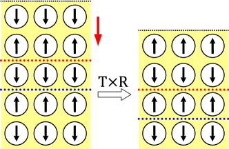
Figure 1: Example of a bulk space group operation producing a degenerate configuration at the surface. An antitranslation $T\times R$, where $T$ is a pure translation normal to the surface (red arrow) and $R$ is time reversal, “cuts off” an atomic layer at the surface of a tetragonal lattice with layered AFM ordering. This bulk space group operation forbids both magnetoelectricity and equilibrium boundary magnetization. Black dotted line shows the boundary. Red and blue dotted lines show two inequivalent types of boundary/bulk partitioning, which are related by a non-magnetic translation $T$. The boundary moment averaged over these two partition types vanishes, because the two types of atomic steps are degenerate.

This conclusion reflects the fact that the free energy of the system with a boundary depends on the polar vector $\mathbf{n}$ as a macroscopic parameter. Just as in the bulk, the existence of the magnetization at the boundary can be deduced from the reduction of the bulk magnetic point group by the presence of the boundary, because translations do not affect $\mathbf{n}$ or $\mathbf{M}_{b}$. From a different angle, a boundary can generate a magnetization only if its zero value is not protected by macroscopic time-reversal symmetry in the bulk; this singles out the magnetoelectrics.

Thus, equilibrium boundary magnetization of a magnetoelectric is finite unless $\alpha_{zk}=0$ for all $k$ in the reference frame where $\mathbf{n}$ is parallel to the $z$ axis. If this magnetization is finite for the given $\mathbf{n}$, it is also necessarily finite for any particular termination with this orientation, because the magnetic symmetry group of the latter is a subgroup of the former.

Probes that are not surface-sensitive, such as magnetometry with $G\{m_{i}(\mathbf{r})\}=\int m_{i}(\mathbf{r})d^{3}r$, measure the sum of contributions of two film boundaries. The total magnetization is non-zero unless there is a bulk symmetry operation interchanging the boundaries. It is always non-zero if these boundaries are with different materials.

The exchange bias induced in a proximate ferromagnetic film by a magnetoelectric is fundamentally different from the conventional exchange bias, which is due to a small excess magnetic moment “frozen-in” in the AFM during field-cooling. In particular, this non-equilibrium character typically leads to an irreversible decline of the exchange bias as the magnetization of the ferromagnetic layer is repeatedly reversed — the so-called training effect Nogués and Schuller (1999); Nogués et al. (2005). By contrast, the switchable exchange bias observed in Ref. He et al., 2010 is an equilibrium property and does not exhibit the training effect.

Since the effect of the boundary is comparable to that of $\mathbf{E}$ of the crystal-field scale, even simple extrapolation suggests that the induced magnetic moments at the boundary can be a few orders of magnitude larger than those achievable due to the bulk magnetoelectric effect. In fact, some mechanisms do not contain any small parameters and are capable of producing magnetizations of the order of a few Bohr magnetons per boundary site. I now classify these mechanisms.

All mechanisms producing linear magnetoelectric response in the bulk Fiebig (2005) can generate boundary magnetization as well; these include changes in (A) the $g$-tensor (here we can also include hybridization-induced changes of the spin moment), (B) the single-ion anisotropy tensor, (C) the intrasublattice symmetric coupling (including Heisenberg exchange and dipolar interactions), and (D) the Dzyaloshinsky-Moriya Dzyaloshinskii (1958); Moriya (1960) exchange coupling induced by $\mathbf{E}$ or by the boundary. All of these except C involve relativistic terms in the Hamiltonian.

Consider the usual case of a collinear AFM. Mechanism C is active only if the perturbation breaks the equivalence of the AFM sublattices. This symmetry breaking can be identified by analyzing the so-called black-and-white (Heesch-Shubnikov) point group based on the decoration of the magnetic sites with Ising spin variables instead of axial vectors. If the perturbation (polar vector $\mathbf{E}$ or $\mathbf{n}$) removes all symmetry operations mapping black and white sites onto each other, the AFM sublattices become inequivalent; otherwise they do not. If the black-and-white point group allows Ising ferromagnetism, the true magnetic point group is also ferromagnetic, but the reverse is not necessarily true. In the first case mechanism C is allowed, but in the second case the magnetoelectric response occurs only through spin canting due to a relativistic perturbation. Thus, certain components of the magnetoelectric tensor, and likewise the boundary magnetization for certain directions of $\mathbf{n}$, may have no contribution from mechanism C. For example, consider Cr₂O₃ (magnetic point group $\underline{\overline{3}m}$) with $\mathbf{E}$ or $\mathbf{n}$ oriented parallel to one of the three $U_{2}$ axes or to one of the three $\sigma_{d}$ planes bisecting them. The corresponding symmetry operation is not removed by $\mathbf{E}$ or $\mathbf{n}$; since both $U_{2}$ and $\sigma_{d}$ interchange the AFM sublattices, the latter remain equivalent. However, the appearance of $\mathbf{M}$ parallel to $\mathbf{E}$ or $\mathbf{M}_{b}$ parallel to $\mathbf{n}$ through spin canting is allowed.

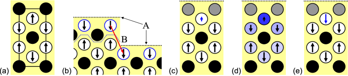
Figure 2: (a): Projected unit cell of the trirutile lattice assumed by magnetoelectric Fe₂TeO₆ (schematic) Kunnmann et al. (1968). Black circles: Te atoms; circles with arrows: Fe atoms with spin directions. O atoms, whose positions make the lattice non-symmorphic, are not shown. (b): Boundary termination cutting between the Fe layers (indicated as type A), including an atomic step. The same AFM sublattice appears at the surface (blue circles). The red arrow shows the bulk symmetry operation (4-fold screw rotation) mapping degenerate atomic steps onto each other. Termination type B (blue dotted line) puts another sublattice at the surface, but it is not related by symmetry and not degenerate with type A. (c)-(e): Mechanisms affecting the boundary magnetization. Termination type B is used as example; Te sites shown in gray may or may not be occupied. (c) Mechanism S1: Changed spin state (blue arrow). (d) Mechanism S2: Unequal thermal averages. Shades of blue and arrow size indicate the degree of thermal disorder. (e) Mechanism S3: Flipped spin direction (blue arrow).

If the equivalence of the AFM sublattices is broken by the boundary, the consequences are far more drastic than in the bulk mechanism C. For any particular boundary termination, even without reconstruction, the sites corresponding to different AFM sublattices are structurally different. For example, all the sites closest to the boundary can have spins “down,” while there is no equivalent termination with boundary spins “up.” The situation is illustrated in Fig. 2b using Fe₂TeO₆ (magnetic point group $4/\underline{mmm}$) as an example. In this figure, terminations A (with boundary spins up) and B (with boundary spins down) are structurally distinct, and therefore they occur with different probabilities in equilibrium. Even if they did appear with equal weights, they are inequivalent magnetically, and don’t generally add up to zero. Indeed, there are several mechanisms leading to the deviation of the average magnetic moments on the boundary sites from the bulk ones (see Fig. 2c-2e): (S1) Different local environment of the magnetic sites near the boundary leads to a different local magnetic moment, and perhaps even a different atomic multiplet. (S2) Since the translational symmetry is broken by the boundary, any symmetric exchange interaction (even purely intersublattice one) leads to different thermal averages at the boundary. (S3) The exchange coupling near the boundary can be so different from the bulk that the AFM ordering pattern can change to ferrimagnetic there. Mechanism S1 can be viewed as a boundary analog of bulk mechanism A, and S2 is the boundary counterpart of mechanism C. S1 and S2 are always present if the black-white symmetry is broken. Apart from these mechanisms affecting the magnitudes of the local moments, the coupling of these moments to the external probe can be different. For example, in the exchange bias setup, the sites closest to the boundary are expected to have the strongest exchange coupling to the proximate ferromagnet.

The bulk linear magnetoelectric effect appears in the free energy expansion as a second-rank tensor $\alpha_{ik}$. This is not the case for the equilibrium boundary magnetization. Since the free energy is a non-analytic function of $\mathbf{n}$ Landau and Lifshitz (1980), the boundary magnetization, given by its field derivative, is also non-analytic. Thus, even if the AFM sublattices are equivalent for some symmetric directions of $\mathbf{n}$, forbidding mechanisms S1-S3 for these orientations, these mechanisms can still generate large boundary magnetization for less symmetric orientations.

Boundary magnetization $\mathbf{M}_{b}$ vanishes at the bulk Néel temperature, but different mechanisms can be partially distinguished experimentally based on its temperature dependence. The thermal mechanism S2 can lead to a non-monotonic contribution with a maximum, similar to the bulk behavior of mechanism C (cf. $\alpha_{zz}$ in Cr₂O₃). Other mechanisms should lead to $\mathbf{M}_{b}$ monotonically decreasing with $T$. All these mechanisms do not contain any small parameters and can produce $\mathbf{M}_{b}$ of the order of a few Bohr magnetons per boundary site. The non-monotonic temperature dependence of the exchange bias field observed in the heterostructure of Ref. He et al. (2010) suggests that mechanism S2 plays an important role at the Cr₂O₃(0001)/Pd interface.

Roughness-insensitive mechanisms based on Dzyaloshinskii-Moriya interaction at the compensated interface were proposed Dong et al. (2009) to explain the exchange bias induced by single-domain multiferroic BiFeO₃ in a proximate FM Martin et al. (2008). They are, however, fundamentally different from all the mechanisms discussed here, because BiFeO₃ is weakly ferromagnetic in the bulk, and also its $\mathbf{M}$ and $\mathbf{P}$ are not linearly coupled Ederer and Spaldin (2005). Therefore, the boundary does not induce additional magnetization components that are forbidden in the bulk.

Much attention is devoted to the search of a room-temperature multiferroic material with linear coupling between the electric polarization $\mathbf{P}$ and magnetization $\mathbf{M}$, because its $\mathbf{M}$ could be switched along with $\mathbf{P}$ by electric field only Eerenstein et al. (2006); Ramesh and Spaldin (2007); Cheong and Mostovoy (2007); Bibes and Barthélémy (2008); Fennie (2008). The paraelectric phase of such a material is a magnetoelectric AFM Fox and Scott (1977); Fennie (2008). The desirable geometry involves voltage applied across the multiferroic film, with $\mathbf{E}$ normal to its surface Bibes and Barthélémy (2008). Equilibrium magnetization $\mathbf{M}_{b}$ necessarily exists at the boundary of such a material. This $\mathbf{M}_{b}$ has the same components as the bulk $\mathbf{M}$ coupled to $\mathbf{P}$, but $\mathbf{M}_{b}$ is coupled to the bulk AFM order parameter. Ferroelectric switching directly switches only the part of $\mathbf{M}$ linearly coupled to $\mathbf{P}$, but not $\mathbf{M}_{b}$. In addition, the states with parallel or antiparallel $\mathbf{M}_{b}$ and $\mathbf{M}$ are non-degenerate, meaning that one of them is metastable or even unstable. Thus, the presence of intrinsic boundary magnetization may hamper purely electric magnetization switching using a multiferroic with linear coupling of $\mathbf{P}$ and $\mathbf{M}$.

Equilibrium boundary magnetization of magnetoelectric AFMs has far-reaching consequences for the design of magnetic nanostructures. First, very large exchange bias fields should be achievable in magnetoelectric/ferromagnet bilayers, comparable to the estimates for a fully uncompensated AFM interface Meiklejohn (1962); Kiwi (2001). Second, magnetoelectric AFMs are precisely the materials that can be switched between the time-reversed AFM domain variants by a simultaneous application of $\mathbf{E}$ and $\mathbf{B}$ fields Schmid (2008); Martin and Anderson (1966), thereby switching the boundary magnetization and the exchange bias field He et al. (2010). The $\mathbf{B}$ field may be permanent, while $\mathbf{E}$ may be provided by a voltage pulse across the magnetoelectric film. Since no depolarizing fields or elastic strains are involved, the AFM domains are stable, and this switching is fully non-volatile. Some device architectures based on the magnetoelectric active layer, where the operation is based on the linear bulk magnetoelectric response, were described by Binek and Doudin Binek and Doudin (2005). These architectures are greatly facilitated by the existence of a switchable equilibrium boundary magnetization, which moreover allows the AFM domain state to be used as a switchable state variable.

In summary, symmetry requires that magnetoelectric antiferromagnets possess a finite boundary magnetization in thermodynamic equilibrium. This magnetization is particularly large if the boundary breaks the equivalence of the antiferromagnetic sublattices; specific microscopic mechanisms have been classified. This understanding will hopefully stimulate further studies of boundary magnetization of magnetoelectrics and its exploitation in nanoelectronic devices.

This work was supported by NSF MRSEC, the Nanoelectronics Research Initiative, and Nebraska Research Initiative. The author is a Cottrell Scholar of Research Corporation.

References

- Landau et al. (1984) L. D. Landau, E. M. Lifshitz, and L. P. Pitaevskii, Electrodynamics of continuous media (Butterworth-Heinemann, Oxford, 1984), sec. 51.
- Fiebig (2005) M. Fiebig, J. Phys. D: Appl. Phys. 38, R123 (2005).
- Schmid (2008) H. Schmid, J. Phys.: Condens. Matter 20, 434201 (2008).
- Dzyaloshinskii (1960) I. E. Dzyaloshinskii, Sov. Phys. JETP 10, 628 (1960).
- Eerenstein et al. (2006) W. Eerenstein, N. D. Mathur, and J. F. Scott, Nature 442, 759 (2006).
- Ramesh and Spaldin (2007) R. Ramesh and N. A. Spaldin, Nature Mater. 6, 21 (2007).
- Cheong and Mostovoy (2007) S.-W. Cheong and M. Mostovoy, Nature Mater. 6, 13 (2007).
- Binek and Doudin (2005) C. Binek and B. Doudin, J. Phys.: Condens. Matter 17, L39 (2005).
- Bibes and Barthélémy (2008) M. Bibes and A. Barthélémy, Nature Mater. 7, 425 (2008).
- Martin et al. (2008) L. W. Martin, Y.-H. Chu, M. B. Holcomb, M. Huijben, P. Yu, S.-J. Han, D. Lee, S. X. Wang, and R. Ramesh, Nano Lett. 8, 2050 (2008).
- Chu et al. (2008) Y.-H. Chu, L. W. Martin, M. B. Holcomb, M. Gajek, S.-J. Han, Q. He, N. Balke, C.-H. Yang, D. Lee, W. Hu, et al., Nature Mater. 7, 478 (2008).
- Meiklejohn (1962) W. H. Meiklejohn, J. Appl. Phys. 33, 1328 (1962).
- Nogués and Schuller (1999) J. Nogués and I. Schuller, J. Magn. Magn. Mater. 192, 203 (1999).
- Nogués et al. (2005) J. Nogués, J. Sort, V. Langlais, V. Skumryev, S. Suriñach, J. S. Muñoz, and M. D. Baró, Phys. Rep. 422, 65 (2005).
- Baek et al. (2010) S. H. Baek, H. W. Jang, C. M. Folkman, Y. L. Li, B. Winchester, J. X. Zhang, Q. He, Y. H. Chu, C. T. Nelson, M. S. Rzchowski, et al., Nature Mater. 9, 309 (2010).
- Fennie (2008) C. J. Fennie, Phys. Rev. Lett. 100, 167203 (2008).
- He et al. (2010) X. He, Y. Wang, N. Wu, A. Caruso, E. Vescovo, K. D. Belashchenko, P. A. Dowben, and C. Binek, Nature Mater. 9, 579 (2010).
- (18) Formally, the thermodynamic limit should be taken with a staggered magnetic field applied at the magnetic sites, whose magnitude is sent to zero afterwards.
- (19) A spin-selective probe with a lower symmetry can generate a finite spin signal even from a magnetically compensated boundary, but we wish to reveal the intrinsic spin asymmetry of the boundary.
- Aizu (1970) K. Aizu, Phys. Rev. B 2, 754 (1970).
- Dzyaloshinskii (1958) I. Dzyaloshinskii, J. Phys. Chem. Solids 4, 241 (1958).
- Moriya (1960) T. Moriya, Phys. Rev. 120, 91 (1960).
- Kunnmann et al. (1968) W. Kunnmann, S. L. Placa, L. M. Corliss, J. M. Hastings, and E. Banks, J. Phys. Chem. Solids 29, 1359 (1968).
- Landau and Lifshitz (1980) L. D. Landau and E. M. Lifshitz, Statistical physics (Butterworth-Heinemann, Oxford, 1980), sec. 155.
- Dong et al. (2009) S. Dong, K. Yamauchi, S. Yunoki, R. Yu, S. Liang, A. Moreo, J.-M. Liu, S. Picozzi, and E. Dagotto, Phys. Rev. Lett. 103, 127201 (2009).
- Ederer and Spaldin (2005) C. Ederer and N. A. Spaldin, Phys. Rev. B 71, 060401 (2005).
- Fox and Scott (1977) D. L. Fox and J. F. Scott, J. Phys. C 10, L329 (1977).
- Kiwi (2001) M. Kiwi, J. Magn. Magn. Mater. 234, 584 (2001).
- Martin and Anderson (1966) T. J. Martin and J. C. Anderson, IEEE Trans. Magn. 2, 446 (1966).