Anti-Coarsening and Complex Dynamics of Step Bunches on Vicinal Surfaces during Sublimation

Marian Ivanov Institut für Theoretische Physik, Universität zu Köln, 50937 Köln, Germany    Vladislav Popkov Interdisziplinäres Zentrum für komplexe Systeme, Rheinische Friedrich-Wilhelms-Universität Bonn, 53117 Bonn, Germany Dipartimento di Fisica Teorica ”E. R. Caianiello”, Università degli Studi di Salerno, Salerno, Italy    Joachim Krug Institut für Theoretische Physik, Universität zu Köln, 50937 Köln, Germany
Abstract

A sublimating vicinal crystal surface can undergo a step bunching instability when the attachment-detachment kinetics is asymmetric, in the sense of a normal Ehrlich-Schwoebel effect. Here we investigate this instability in a model that takes into account the subtle interplay between sublimation and step-step interactions, which breaks the volume-conserving character of the dynamics assumed in previous work. On the basis of a systematically derived continuum equation for the surface profile, we argue that the non-conservative terms pose a limitation on the size of emerging step bunches. This conclusion is supported by extensive simulations of the discrete step dynamics, which show breakup of large bunches into smaller ones as well as arrested coarsening and periodic oscillations between states with different numbers of bunches.

pacs:
05.70.Np, 68.35.Ct, 81.16.Rf

I Introduction

We consider a vicinal crystal surface of parallel oriented steps in contact with the vapor phase of the same material. By varying the sample temperature the crystal can start to sublimate or grow in the step flow mode Jeong1999 ; Krug2005 ; PierreLouis2005 ; Krug2010 . In the presence of an asymmetry in the kinetics at the steps bordering a terrace, perturbations in the step flow may grow such that the step profile undergoes a step bunching instability. There are two questions of general interest. First, what are the physical conditions required for such an instability? And second, how does the surface morphology evolve once the instability has appeared?

In recent years many groups have addressed these questions within the framework of the standard model first introduced by Burton, Cabrera and Frank Burton1951 (BCF). In the absence of additional effects such as electromigration Stoyanov1991 ; Sato1999 or strain Tersoff1995 , the basic stability scenario is simple: Preferential attachment to ascending steps (a normal Ehrlich-Schwoebel effect) leads to step bunching during sublimation, while preferential attachment to descending steps (an inverse Ehrlich-Schwoebel effect) implies step bunching during growth Schwoebel1969 ; Pimpinelli1994 ; Uwaha1995 ; Sato2001 ; Xie2002 ; Slanina2005 . The symmetry between growth and sublimation suggested by this result is however not complete PierreLouis2003 ; Fok2007 : Whereas the deposition flux in a growth experiment is an externally controlled parameter that is independent of the surface morphology, the sublimation flux is driven by the surface free energy and hence depends on the curvature of the surface. As a consequence, the time evolution of the surface profile conserves the volume of the film (apart from a constant rate of increase) in the case of growth but not in the case of sublimation Krug1997 .

In the present paper we explore the consequences of the non-conservative nature of the sublimation dynamics for the linear and nonlinear evolution of step bunches. We base our treatment on the BCF model in the quasistatic limit including sublimation, the Ehrlich-Schwoebel effect and step-step interactions. In previous work we have developed a detailed continuum description of step bunching in this system, in which non-conservative terms arising from the interplay between sublimation and capillarity were however neglected KrugPimpinelli ; popkovkrug . Here these terms are explicitly included and their effect is studied both in the discrete dynamics of individual steps and on the continuum level.

Although the coefficients of the non-conserved terms are usually small under physically realistic conditions, they turn out to have dramatic consequences. Most importantly, whereas step bunches in conserved systems typically coarsen indefinitely, here we find that coarsening is arrested when a maximal bunch size has been reached. Conversely, if the system of steps is started in an initial condition representing a single large bunch, anti-coarsening involving the breakup of the initial bunch into several small bunches is observed. More complex scenarios in which the number of bunches in the system varies periodically in time are also possible.

The article is organized as follows. In the next section we briefly introduce the BCF-model which forms the starting point of our work. In Section III the discrete equations of motion for the steps are presented and the results of a linear stability analysis are described. In Section IV we derive a continuum evolution equation along the lines of KrugPimpinelli ; JoachimKim and provide a partial analysis which suggests the existence of an upper bound on the size of step bunches in the non-conserved case. Section V is devoted to the numerical exploration of the various scenarios of nonlinear evolution in the discrete step dynamics, and some conclusions are presented in Section VI. Details of the analytic calculations are collected in the Appendices.

II Model

On the mesoscopic scale the surface can be reduced to a one-dimensional train of steps. The BCF model is based on a non-conserved diffusion equation for the concentration profile ni(x,t)subscript𝑛𝑖𝑥𝑡n_{i}(x,t) on the i𝑖i’th terrace (see Fig.1), which reads

ni(x,t)t=Ds2ni(x,t)x2ni(x,t)τ+F.subscript𝑛𝑖𝑥𝑡𝑡subscript𝐷𝑠superscript2subscript𝑛𝑖𝑥𝑡superscript𝑥2subscript𝑛𝑖𝑥𝑡𝜏𝐹\frac{\partial n_{i}(x,t)}{\partial t}=D_{s}\frac{\partial^{2}n_{i}(x,t)}{\partial x^{2}}-\frac{n_{i}(x,t)}{\tau}+F. (1)

The terms on the right hand side correspond to the three processes sketched in Fig. 1. The first one is a diffusion term with surface diffusion coefficient Dssubscript𝐷𝑠D_{s}, the second term includes the losses of adatoms during sublimation with desorption rate 1/τ1𝜏1/\tau, and the last one describes the gain of adatoms from the surrounding gas phase with deposition rate F𝐹F. Together diffusion and desorption give rise to the diffusion length lD=Dsτsubscript𝑙𝐷subscript𝐷𝑠𝜏l_{D}=\sqrt{D_{s}\tau}, defined as the distance an adatom travels before it desorbs (in the absence of other processes).

Refer to caption

Figure 1: (Color online) Sketch of the elementary processes in the Burton-Cabrera-Frank model

Solving (1) in the quasistatic limit ni/t=0subscript𝑛𝑖𝑡0\partial n_{i}/\partial t=0 one can find the general solution. The constants of integration are specified through the following boundary conditions. We consider a terrace of width l𝑙l confined between two steps at the positions x=±l/2𝑥plus-or-minus𝑙2x=\pm l/2. The condition of mass conservation on both bounding steps defines the system of differential equations

Dsn(x)x=+k[n(x)neq(x)],atx=l2,formulae-sequencesubscript𝐷𝑠𝑛𝑥𝑥subscript𝑘delimited-[]𝑛𝑥subscript𝑛𝑒𝑞𝑥at𝑥𝑙2\displaystyle D_{s}\frac{\partial n(x)}{\partial x}=+k_{-}[n(x)-n_{eq}(x)],\ \ \ \text{at}\ x=-\frac{l}{2},
Dsn(x)x=k+[n(x)neq(x)],atx=+l2.formulae-sequencesubscript𝐷𝑠𝑛𝑥𝑥subscript𝑘delimited-[]𝑛𝑥subscript𝑛𝑒𝑞𝑥at𝑥𝑙2\displaystyle D_{s}\frac{\partial n(x)}{\partial x}=-k_{+}[n(x)-n_{eq}(x)],\ \ \ \text{at}\ x=+\frac{l}{2}. (2)

On the left hand sides the adatom fluxes from the terrace toward the steps appear, which are compensated by the attachment and detachment of adatoms that are caused by the difference between the actual concentration at the step relative to the equilibrium concentrations.

The system (II) contains two additional effects. First, the proportionality constants ksubscript𝑘k_{-} and k+subscript𝑘k_{+} are the attachment/detachment kinetic coefficients, where index the ++ (-) denotes the coefficient corresponding to attachment/detachment from below (above) the step. In general the k±subscript𝑘plus-or-minusk_{\pm} are unequal. The case k+>ksubscript𝑘subscript𝑘k_{+}>k_{-} corresponds to the so called Ehrlich-Schwoebel effect Schwoebel1969 while in the converse case we speak about an inverse Ehrlich-Schwoebel effect Sato2001 ; Xie2002 ; Slanina2005 . Analogous to the diffusion length we define the kinetic lengths l±=Ds/k±subscript𝑙plus-or-minussubscript𝐷𝑠subscript𝑘plus-or-minusl_{\pm}=D_{s}/k_{\pm} Krug2005 and further their dimensionless versions l±/lD=l±subscript𝑙plus-or-minussubscript𝑙𝐷superscript𝑙plus-or-minusl_{\pm}/l_{D}=l^{\pm} (note the different placement of the indices ±plus-or-minus\pm).

The second effect included in the boundary conditions (II) are the (repulsive) step-step interactions. The expression for the equilibrium concentration is given by the usual grand canonical formula, which we use in the first order approximation

neq(xi)neq0(1+μi/kBT).subscript𝑛𝑒𝑞subscript𝑥𝑖subscriptsuperscript𝑛0𝑒𝑞1subscript𝜇𝑖subscript𝑘𝐵𝑇n_{eq}(x_{i})\approx n^{0}_{eq}(1+\mu_{i}/k_{B}T). (3)

The chemical potential μisubscript𝜇𝑖\mu_{i} at the i𝑖ith step depends on the widths li=xixi1subscript𝑙𝑖subscript𝑥𝑖subscript𝑥𝑖1l_{i}=x_{i}-x_{i-1} of the neighboring terraces according to the law

μikBT=g[l3(li)3l3(li1)3]gνi,subscript𝜇𝑖subscript𝑘𝐵𝑇𝑔delimited-[]superscript𝑙3superscriptsubscript𝑙𝑖3superscript𝑙3superscriptsubscript𝑙𝑖13𝑔subscript𝜈𝑖\frac{\mu_{i}}{k_{B}T}=-g\left[\frac{l^{3}}{(l_{i})^{3}}-\frac{l^{3}}{(l_{i-1})^{3}}\right]\equiv g\nu_{i}, (4)

which was first derived theoretically for entropic repulsion grubermullins . The ubiquity of repulsive step-step interactions is well confirmed by experiments, which also show that the dominant contribution to the amplitude g𝑔g arises from elastic interactions Jeong1999 ; giesen .

In order to render g𝑔g dimensionless we have rescaled the terrace widths in (4) by the mean terrace width l𝑙l. Note that our definition of g𝑔g differs from the conventional notation, where the strength of step interactions is quantified by the coefficient of the cubic term in the expansion of the surface free energy in the surface miscut θ𝜃\theta, the angle formed by the vicinal surface relative to the high symmetry orientation Jeong1999 . Denoting the latter coefficient by g~~𝑔\tilde{g}, the relation between the two reads LiuWeeks

g=2g~ΩkBT|tanθ|3,𝑔2~𝑔Ωsubscript𝑘𝐵𝑇superscript𝜃3g=\frac{2\tilde{g}\Omega}{k_{B}T}|\tan\theta|^{3},

where ΩΩ\Omega denotes the atomic area. To give an impression of the order of magnitude of g𝑔g, for the Si(111) surface at 900oo{}^{\textrm{o}} the estimate g~0.05~𝑔0.05\tilde{g}\approx 0.05 eV/Å2 Jeong1999 yields g10|tanθ|35×105𝑔10superscript𝜃35superscript105g\approx 10|\tan\theta|^{3}\approx 5\times 10^{-5} for a typical miscut of 1oo{}^{\textrm{o}}.

Refer to caption

Figure 2: Sketch of the contributions to the velocity of the i𝑖i-th step.

Together Eqs.(1,II,3,4) specify the boundary value problem for the ni(x)subscript𝑛𝑖𝑥n_{i}(x). Having computed the concentration profiles we can use Fick’s first law to find the mass fluxes from below (f+i1superscriptsubscript𝑓𝑖1f_{+}^{i-1}) and above (fisuperscriptsubscript𝑓𝑖f_{-}^{i}) the i𝑖i-th step, which sum to give its velocity vi=dxidt=fi+f+i1subscript𝑣𝑖𝑑subscript𝑥𝑖𝑑𝑡superscriptsubscript𝑓𝑖superscriptsubscript𝑓𝑖1v_{i}=\frac{dx_{i}}{dt}=f_{-}^{i}+f_{+}^{i-1} (see Fig. 2).

III Discrete view

III.1 Equations of step motion

In Appendix A.1 we derive the concentration profile ni(x)subscript𝑛𝑖𝑥n_{i}(x) for the case of sublimation (F=0𝐹0F=0) with step-step repulsion and the Ehrlich-Schwoebel effect in the quasistatic limit, see Eq. (17) and Eq. (A.1), which yields

ni(x)subscript𝑛𝑖𝑥\displaystyle n_{i}(x) =\displaystyle= neq0[(l+1)(1+μikT)eli2lD+(l+1)(1+μi+1kT)eli2lD(l+l+1)sinhlilD+(l+l+)coshlilD]exlD2+limit-fromsubscriptsuperscript𝑛0𝑒𝑞delimited-[]superscript𝑙11subscript𝜇𝑖𝑘𝑇superscript𝑒subscript𝑙𝑖2subscript𝑙𝐷superscript𝑙11subscript𝜇𝑖1𝑘𝑇superscript𝑒subscript𝑙𝑖2subscript𝑙𝐷superscript𝑙superscript𝑙1subscript𝑙𝑖subscript𝑙𝐷superscript𝑙superscript𝑙subscript𝑙𝑖subscript𝑙𝐷superscript𝑒𝑥subscript𝑙𝐷2\displaystyle n^{0}_{eq}\left[\frac{(l^{+}-1)(1+\frac{\mu_{i}}{kT})e^{-\frac{l_{i}}{2l_{D}}}+(l^{-}+1)(1+\frac{\mu_{i+1}}{kT})e^{\frac{l_{i}}{2l_{D}}}}{(l^{+}l^{-}+1)\sinh\frac{l_{i}}{l_{D}}+(l^{-}+l^{+})\cosh\frac{l_{i}}{l_{D}}}\right]\frac{e^{\frac{x}{l_{D}}}}{2}+ (5)
+\displaystyle+ neq0[(l1)(1+μikT)eli2lD+(l++1)(1+μi+1kT)eli2lD(l+l+1)sinhlilD+(l+l+)coshlilD]exlD2.subscriptsuperscript𝑛0𝑒𝑞delimited-[]superscript𝑙11subscript𝜇𝑖𝑘𝑇superscript𝑒subscript𝑙𝑖2subscript𝑙𝐷superscript𝑙11subscript𝜇𝑖1𝑘𝑇superscript𝑒subscript𝑙𝑖2subscript𝑙𝐷superscript𝑙superscript𝑙1subscript𝑙𝑖subscript𝑙𝐷superscript𝑙superscript𝑙subscript𝑙𝑖subscript𝑙𝐷superscript𝑒𝑥subscript𝑙𝐷2\displaystyle n^{0}_{eq}\left[\frac{(l^{-}-1)(1+\frac{\mu_{i}}{kT})e^{-\frac{l_{i}}{2l_{D}}}+(l^{+}+1)(1+\frac{\mu_{i+1}}{kT})e^{\frac{l_{i}}{2l_{D}}}}{(l^{+}l^{-}+1)\sinh\frac{l_{i}}{l_{D}}+(l^{-}+l^{+})\cosh\frac{l_{i}}{l_{D}}}\right]\frac{e^{-\frac{x}{l_{D}}}}{2}.

From (5) we find the following discrete equations of step motion (see Appendix A.2)

dxidt𝑑subscript𝑥𝑖𝑑𝑡\displaystyle\frac{dx_{i}}{dt} =\displaystyle= ΩDsneq0lD[(1+μikT)(lsinhli1lD+coshli1lD)(1+μi1kT)(l+l+1)sinhli1lD+(l+l+)coshli1lD]+limit-fromΩsubscript𝐷𝑠subscriptsuperscript𝑛0𝑒𝑞subscript𝑙𝐷delimited-[]1subscript𝜇𝑖𝑘𝑇superscript𝑙subscript𝑙𝑖1subscript𝑙𝐷subscript𝑙𝑖1subscript𝑙𝐷1subscript𝜇𝑖1𝑘𝑇superscript𝑙superscript𝑙1subscript𝑙𝑖1subscript𝑙𝐷superscript𝑙superscript𝑙subscript𝑙𝑖1subscript𝑙𝐷\displaystyle\frac{\Omega D_{s}n^{0}_{eq}}{l_{D}}\left[\frac{\left(1+\frac{\mu_{i}}{kT}\right)\left(l^{-}\sinh\frac{l_{i-1}}{l_{D}}+\cosh\frac{l_{i-1}}{l_{D}}\right)-\left(1+\frac{\mu_{i-1}}{kT}\right)}{(l^{+}l^{-}+1)\sinh\frac{l_{i-1}}{l_{D}}+(l^{-}+l^{+})\cosh\frac{l_{i-1}}{l_{D}}}\right]+ (6)
+\displaystyle+ ΩDsneq0lD[(1+μikT)(l+sinhlilD+coshlilD)(1+μi+1kT)(l+l+1)sinhlilD+(l+l+)coshlilD].Ωsubscript𝐷𝑠subscriptsuperscript𝑛0𝑒𝑞subscript𝑙𝐷delimited-[]1subscript𝜇𝑖𝑘𝑇superscript𝑙subscript𝑙𝑖subscript𝑙𝐷subscript𝑙𝑖subscript𝑙𝐷1subscript𝜇𝑖1𝑘𝑇superscript𝑙superscript𝑙1subscript𝑙𝑖subscript𝑙𝐷superscript𝑙superscript𝑙subscript𝑙𝑖subscript𝑙𝐷\displaystyle\frac{\Omega D_{s}n^{0}_{eq}}{l_{D}}\left[\frac{\left(1+\frac{\mu_{i}}{kT}\right)\left(l^{+}\sinh\frac{l_{i}}{l_{D}}+\cosh\frac{l_{i}}{l_{D}}\right)-\left(1+\frac{\mu_{i+1}}{kT}\right)}{(l^{+}l^{-}+1)\sinh\frac{l_{i}}{l_{D}}+(l^{-}+l^{+})\cosh\frac{l_{i}}{l_{D}}}\right].

The step velocities (6) include all three length scales lDsubscript𝑙𝐷l_{D}, l±subscript𝑙plus-or-minusl_{\pm}, l𝑙l and the functional dependence is quite complicated. From now on we therefore consider the case of attachment/detachment limited kinetics (lDl±lmuch-greater-thansubscript𝑙𝐷subscript𝑙plus-or-minusmuch-greater-than𝑙l_{D}\gg l_{\pm}\gg l), which is commonly assumed for the Si(111) surface LiuWeeks . In this limit Eq. (6) can be reduced to the following form (see Appendix A.4):

dxidt=(1+gνi)Re(1+b2li1+1b2li)+URe(2νiνi1νi+i),𝑑subscript𝑥𝑖𝑑𝑡1𝑔subscript𝜈𝑖subscript𝑅𝑒1𝑏2subscript𝑙𝑖11𝑏2subscript𝑙𝑖𝑈subscript𝑅𝑒2subscript𝜈𝑖subscript𝜈𝑖1subscript𝜈𝑖𝑖\displaystyle\frac{dx_{i}}{dt}=\left(1+g\nu_{i}\right)R_{e}\left(\frac{1+b}{2}l_{i-1}+\frac{1-b}{2}l_{i}\right)+UR_{e}(2\nu_{i}-\nu_{i-1}-\nu_{i+i}), (7)

with the abbreviations

b𝑏\displaystyle b =\displaystyle= k+kk+k+=ll+l+l+,subscript𝑘subscript𝑘subscript𝑘subscript𝑘subscript𝑙subscript𝑙subscript𝑙subscript𝑙\displaystyle\frac{k_{+}-k_{-}}{k_{-}+k_{+}}\ =\frac{l_{-}-l_{+}}{l_{-}+l_{+}},
Resubscript𝑅𝑒\displaystyle R_{e} =\displaystyle= Ωneq0τΩsubscriptsuperscript𝑛0𝑒𝑞𝜏\displaystyle\frac{\Omega n^{0}_{eq}}{\tau}\,
U𝑈\displaystyle U =\displaystyle= gτkk+k+k+=glD2l+l+.𝑔𝜏subscript𝑘subscript𝑘subscript𝑘subscript𝑘𝑔superscriptsubscript𝑙𝐷2subscript𝑙subscript𝑙\displaystyle g\tau\frac{k_{-}k_{+}}{k_{-}+k_{+}}\ =\frac{gl_{D}^{2}}{l_{-}+l_{+}}. (8)

Here Resubscript𝑅𝑒R_{e} represents the constant desorption rate of a homogeneous step train, where dxi/dt=Rel𝑑subscript𝑥𝑖𝑑𝑡subscript𝑅𝑒𝑙dx_{i}/dt=R_{e}l, b𝑏b is a dimensionless measure for the strength of the Ehrlich-Schwoebel effect and U𝑈U describes the strength of the relaxation due to the step-step repulsion. Note that U𝑈U has the dimension of a length.

In previous work on step bunching during sublimation, where the instability is induced either by the Ehrlich-Schwoebel effect or by electromigration, the factor 1+gνi1𝑔subscript𝜈𝑖1+g\nu_{i} of the first term on the right hand side of (7) was tacitly replaced by unity KrugPimpinelli ; popkovkrug ; LiuWeeks ; slava . The approximation 1+gνi11𝑔subscript𝜈𝑖11+g\nu_{i}\approx 1 may seem plausible because, as we have seen, g1much-less-than𝑔1g\ll 1 under typical experimental conditions. However, it is clear from the structure of (7) that the presence of this factor changes the nature of the problem in a qualitative way: Considering periodic boundaries for the step train of M𝑀M steps, so that xM+1=x1+Mlsubscript𝑥𝑀1subscript𝑥1𝑀𝑙x_{M+1}=x_{1}+Ml, and taking the sum of (7) over one period one obtains the configuration-independent constant Ml𝑀𝑙Ml on the right hand size only when the term gνi𝑔subscript𝜈𝑖g\nu_{i} (referred to in the following as the g𝑔g-term) is neglected. The full system (7) is fundamentally non-conservative.

On the other hand, the step dynamics is exactly conservative for the case of pure growth (F>0,τformulae-sequence𝐹0𝜏F>0,\tau\rightarrow\infty) in the same limit in which (7) was derived. In the case of growth we obtain

dxidtFΩ(1+b2li1+1b2li)+U~(2νiνi1νi+i)𝑑subscript𝑥𝑖𝑑𝑡𝐹Ω1𝑏2subscript𝑙𝑖11𝑏2subscript𝑙𝑖~𝑈2subscript𝜈𝑖subscript𝜈𝑖1subscript𝜈𝑖𝑖\displaystyle\frac{dx_{i}}{dt}\approx-F\Omega\left(\frac{1+b}{2}l_{i-1}+\frac{1-b}{2}l_{i}\right)+\tilde{U}(2\nu_{i}-\nu_{i-1}-\nu_{i+i}) (9)

which is precisely the conservative version of (7) with the sublimation rate Resubscript𝑅𝑒R_{e} replaced by the (negative) growth rate FΩ𝐹ΩF\Omega and with U~=(gΩneq0kk+)/(k+k+)~𝑈𝑔Ωsubscriptsuperscript𝑛0𝑒𝑞subscript𝑘subscript𝑘subscript𝑘subscript𝑘\tilde{U}=(g\Omega n^{0}_{eq}k_{-}k_{+})/(k_{-}+k_{+}). This implies a basic asymmetry between sublimation and growth, the consequences of which will be explored in the following. To this end we will consider U𝑈U and g𝑔g in (7) as independent parameters, in spite of the proportionality between U𝑈U and g𝑔g. The conserved model (9) is thus included in (7) as the limiting case g=0,U>0formulae-sequence𝑔0𝑈0g=0,U>0.

III.2 Linear stability analysis

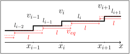
The instability form of a step train is step bunching and in this section we look for the linear instability condition as a function of the control parameters. Let us consider the regular situation of equidistant terrace widths l𝑙l and steps moving with a constant velocity veq=f(l)+f+(l)subscript𝑣𝑒𝑞subscript𝑓𝑙subscript𝑓𝑙v_{eq}=f_{-}(l)+f_{+}(l), see Fig. 3. Now, we disturb the positions of the steps by a small time dependent perturbation εn(t)subscript𝜀𝑛𝑡\varepsilon_{n}(t):

xn(t)=nl+veqt+εn(t).subscript𝑥𝑛𝑡𝑛𝑙subscript𝑣𝑒𝑞𝑡subscript𝜀𝑛𝑡\displaystyle x_{n}(t)=nl+v_{eq}t+\varepsilon_{n}(t).

Refer to caption

Figure 3: (Color online) Illustration of the linear stability analysis. The dotted line shows a homogeneous step train with constant terrace width l𝑙l and constant step velocity veqsubscript𝑣𝑒𝑞v_{eq}, the full line shows a perturbed step train.

Refer to caption

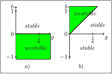
Figure 4: (Color online) Stability diagram in the (g,b)𝑔𝑏(g,b)-plane for a) growth and b) sublimation.

Through substitution of εn(t)subscript𝜀𝑛𝑡\varepsilon_{n}(t) by the Fourier expression ε0eikn+ω(k)tsubscript𝜀0superscript𝑒𝑖𝑘𝑛𝜔𝑘𝑡\varepsilon_{0}e^{ikn+\omega(k)t} we derive a dispersion relation ω(k)𝜔𝑘\omega(k). For instability the real part of ω(k)𝜔𝑘\omega(k) has to be positive, i.e.

Re[ω(k)]A2k2+A4k4𝑅𝑒delimited-[]𝜔𝑘subscript𝐴2superscript𝑘2subscript𝐴4superscript𝑘4\displaystyle Re[\omega(k)]\approx A_{2}k^{2}+A_{4}k^{4}

with A2>0subscript𝐴20A_{2}>0. In Appendix A.3, Eq.(24), we find:

Re[ω(k)]=ΩDsneq0lD2[(k+k)2(k++k)3g]k23gΩDsneq0lkk+k+k+k4.𝑅𝑒delimited-[]𝜔𝑘Ωsubscript𝐷𝑠subscriptsuperscript𝑛0𝑒𝑞subscriptsuperscript𝑙2𝐷delimited-[]subscript𝑘subscript𝑘2subscript𝑘subscript𝑘3𝑔superscript𝑘23𝑔Ωsubscript𝐷𝑠subscriptsuperscript𝑛0𝑒𝑞𝑙subscript𝑘subscript𝑘subscript𝑘subscript𝑘superscript𝑘4\displaystyle Re[\omega(k)]=\frac{\Omega D_{s}n^{0}_{eq}}{l^{2}_{D}}\left[\frac{(k_{+}-k_{-})}{2(k_{+}+k_{-})}-3g\right]k^{2}-3g\frac{\Omega D_{s}n^{0}_{eq}}{l}\frac{k_{-}k_{+}}{k_{-}+k_{+}}k^{4}.

For the case of sublimation in the limit of long wavelengths (small k𝑘k) the instability condition is b>6g𝑏6𝑔b>6g. This means that the existence of an Ehrlich-Schwoebel effect alone (b>0𝑏0b>0) is not sufficient to cause an instability: Due to the step-step interactions there is a lower limit 6g6𝑔6g on the strength of the kinetic asymmetry which has to be overcome to cause step bunching during sublimation. This effect was previously reported by Fok, Rosales and Margetis Fok2007 in a more general setting. On the other hand for the case of growth we have the usual linear instability condition of b<0𝑏0b<0, which corresponds to an inverse Ehrlich-Schwoebel effect of arbitrary strengh. The resulting asymmetry between sublimation and growth on the level of linear stability analysis is illustrated in Fig. 4.

IV Continuum description

The continuum evolution equation corresponding to the discrete dynamics (7) has the form

ht+x(3g2(m2)b2m16m3mx+3U2m2(m2)x2)=1+3gb2m(mx)2𝑡𝑥3𝑔2superscript𝑚2𝑏2𝑚16superscript𝑚3𝑚𝑥3𝑈2𝑚superscript2superscript𝑚2superscript𝑥213𝑔𝑏2𝑚superscript𝑚𝑥2\frac{\partial h}{\partial t}+\frac{\partial}{\partial x}\left(-\frac{3g}{2}\left(m^{2}\right)-\frac{b}{2m}-\frac{1}{6m^{3}}\frac{\partial m}{\partial x}+\frac{3U}{2m}\frac{\partial^{2}\left(m^{2}\right)}{\partial x^{2}}\right)=-1+\frac{3gb}{2m}\left(\frac{\partial m}{\partial x}\right)^{2} (10)

where h(x,t)𝑥𝑡h(x,t) is the surface profile, m(x,t)=h/x>0𝑚𝑥𝑡𝑥0m(x,t)=\partial h/\partial x>0 is the slope, and primes denote the derivatives with respect to x𝑥x, e.g. m=m/xsuperscript𝑚𝑚𝑥m^{\prime}=\partial m/\partial x. Here and below we set the step height and the average step-step distance l𝑙l to 111, and rescale time such that the mean sublimation rate Re=1subscript𝑅𝑒1R_{e}=1. The details of the derivation can be found in Appendix B.

For g=0𝑔0g=0, the equation (10) reduces to the one studied in KrugPimpinelli ; popkovkrug . In that case the transformation to a moving frame hh+t𝑡h\to h+t removes the constant mean sublimation rate on the right hand side and gives the equation the form of a conservation law

ht+Jx=0,𝑡𝐽𝑥0\frac{\partial h}{\partial t}+\frac{\partial J}{\partial x}=0, (11)

with a current J𝐽J defined by the terms inside the large parentheses on the left hand side of (10). For g>0𝑔0g>0 we obtain an additional contribution (3g/2)m23𝑔2superscript𝑚2(3g/2)m^{2} to the current, and the manifestly non-conservative term (3gb/2m)(m)23𝑔𝑏2𝑚superscriptsuperscript𝑚2(3gb/2m)(m^{\prime})^{2} appears on the right-hand side of (10). In the following we discuss separately the effects of the conserved and non-conserved contributions that are present when g>0𝑔0g>0.

IV.1 Mechanical analog for symmetric stationary bunches

We first analyze the effect of the conservative term (3g/2)m23𝑔2superscript𝑚2(3g/2)m^{2} on the left hand side of (10). Along the lines of KrugPimpinelli , we consider a stationary solution of (11) with the current given by

J=3g2(m2)b2mm6m3+3U2m(m2)′′.𝐽3𝑔2superscript𝑚2𝑏2𝑚superscript𝑚6superscript𝑚33𝑈2𝑚superscriptsuperscript𝑚2′′\displaystyle J=-\frac{3g}{2}\left(m^{2}\right)-\frac{b}{2m}-\frac{m^{\prime}}{6m^{3}}+\frac{3U}{2m}\left(m^{2}\right)^{\prime\prime}. (12)

For a stationary bunch JJ0<0𝐽subscript𝐽00J\equiv-J_{0}<0. Furthermore we neglect the third term on the right hand side of (12), which breaks the reflection symmetry (xx𝑥𝑥x\rightarrow-x and mm𝑚𝑚m\rightarrow-m). Setting u=m2𝑢superscript𝑚2u=m^{2} (m>0𝑚0m>0) then yields

J0=3g2u+b2u1/23Uu′′2u1/2subscript𝐽03𝑔2𝑢𝑏2superscript𝑢123𝑈superscript𝑢′′2superscript𝑢12\displaystyle J_{0}=\frac{3g}{2}u+\frac{b}{2}u^{-1/2}-\frac{3Uu^{\prime\prime}}{2}u^{-1/2}

or

3U2u′′=J0u1/2+3g2u3/2+b2=dVg(u)du.3𝑈2superscript𝑢′′subscript𝐽0superscript𝑢123𝑔2superscript𝑢32𝑏2𝑑subscript𝑉𝑔𝑢𝑑𝑢\displaystyle\frac{3U}{2}u^{\prime\prime}=-J_{0}u^{1/2}+\frac{3g}{2}u^{3/2}+\frac{b}{2}=-\frac{dV_{g}(u)}{du}. (13)

Equation (13) can be interpreted as Newton’s second law describing a particle coordinate u𝑢u moving in time x𝑥x. In this picture a symmetric bunch of width L𝐿L represents a trajectory of a classical particle moving once back and forth in a potential Vg(u)subscript𝑉𝑔𝑢V_{g}(u) between the boundary values u=0𝑢0u=0 and u=umax𝑢subscript𝑢𝑚𝑎𝑥u=u_{max} in a time L𝐿L. Up to a constant, the potential Vg(u)subscript𝑉𝑔𝑢V_{g}(u) can be found through integration of (13),

Vg(u)=2J03u3/23g5u5/2b2u=V0(u)3g5u5/2.subscript𝑉𝑔𝑢2subscript𝐽03superscript𝑢323𝑔5superscript𝑢52𝑏2𝑢subscript𝑉0𝑢3𝑔5superscript𝑢52\displaystyle V_{g}(u)=\frac{2J_{0}}{3}u^{3/2}-\frac{3g}{5}u^{5/2}-\frac{b}{2}u=V_{0}(u)-\frac{3g}{5}u^{5/2}. (14)

The function (14) contains an additional term compared to the potential V0(u)subscript𝑉0𝑢V_{0}(u) considered in KrugPimpinelli . This term causes a maximum of Vg(u)subscript𝑉𝑔𝑢V_{g}(u) to appear at some usuperscript𝑢u^{\ast}, whereas V0(u)subscript𝑉0𝑢V_{0}(u) grows monotonically for large u𝑢u. This has the following consequence. Let us consider a bunch of M𝑀M steps. For a given set of parameters b𝑏b, g𝑔g and U𝑈U this bunch solution corresponds to a particle trajectory of total energy E𝐸E and a certain maximal slope mmaxsubscript𝑚𝑚𝑎𝑥m_{max} with umax=mmax2<usubscript𝑢𝑚𝑎𝑥superscriptsubscript𝑚𝑚𝑎𝑥2superscript𝑢u_{max}=m_{max}^{2}<u^{\ast}. Now, let us increase the bunch width L𝐿L by adding more and more steps, which increases the energy E𝐸E and the value of umaxsubscript𝑢𝑚𝑎𝑥u_{max}. As umaxusubscript𝑢𝑚𝑎𝑥superscript𝑢u_{max}\to u^{\ast} and EVg(u)𝐸subscript𝑉𝑔superscript𝑢E\to V_{g}(u^{\ast}), the oscillation period L𝐿L of the particle diverges, which implies that the maximum slope mmaxsubscript𝑚𝑚𝑎𝑥m_{max} cannot increase beyond usuperscript𝑢\sqrt{u^{\ast}}. This is in contrast to the case g=0𝑔0g=0, where the maximum slope scales with the number of steps as mmaxM2/3similar-tosubscript𝑚𝑚𝑎𝑥superscript𝑀23m_{max}\sim M^{2/3} and with the bunch width as mmaxL2similar-tosubscript𝑚𝑚𝑎𝑥superscript𝐿2m_{max}\sim L^{2} KrugPimpinelli . Even on the rather crude level of the stationary bunch approximation used in KrugPimpinelli , the presence of the g𝑔g-term in (12) is seen to have a pronounced effect, in that it prevents the unbounded steepening of the bunch profile. In the next subsection we shall see that, when bunch motion is taken into account, the non-conserved nature of the dynamics also prevents the wavelength of the bunch from increasing indefinitely.

IV.2 Moving bunches

In fact step bunches are not stationary, but move both in the horizontal direction (with speed Vsubscript𝑉parallel-toV_{\parallel}) and in the vertical direction (with speed Vsubscript𝑉perpendicular-toV_{\perp}) popkovkrug . A periodic array of moving bunches is obtained from (10) using the travelling wave ansatz

h(x,t)=h(xVt)+Vtt,𝑥𝑡𝑥subscript𝑉parallel-to𝑡subscript𝑉perpendicular-to𝑡𝑡h\left(x,t\right)=h\left(x-V_{\parallel}t\right)+V_{\perp}t-t,

which yields the ordinary differential equation

Vh+V+(3g2(m2)b2mm6m3+3U2m(m2)′′)=3gb2(m)2m.subscript𝑉parallel-tosuperscriptsubscript𝑉perpendicular-tosuperscript3𝑔2superscript𝑚2𝑏2𝑚superscript𝑚6superscript𝑚33𝑈2𝑚superscriptsuperscript𝑚2′′3𝑔𝑏2superscriptsuperscript𝑚2𝑚-V_{\parallel}h^{\prime}+V_{\perp}+\left(-\frac{3g}{2}\left(m^{2}\right)-\frac{b}{2m}-\frac{m^{\prime}}{6m^{3}}+\frac{3U}{2m}\left(m^{2}\right)^{\prime\prime}\right)^{\prime}=\frac{3gb}{2}\frac{\left(m^{\prime}\right)^{2}}{m}. (15)

Here primes denote derivatives with respect to co-moving space coordinate ξ=xVt𝜉𝑥subscript𝑉parallel-to𝑡\xi=x-V_{\parallel}t and m(ξ)=dh/dξ𝑚𝜉𝑑𝑑𝜉m(\xi)=dh/d\xi. We look for periodic solutions h(ξ)=h(ξ+M)𝜉𝜉𝑀h(\xi)=h(\xi+M). Integrating (15) from 00 till M𝑀M, and dividing by M𝑀M we obtain

VV=g3b2M0M(m)2m𝑑ξsubscript𝑉parallel-tosubscript𝑉perpendicular-to𝑔3𝑏2𝑀superscriptsubscript0𝑀superscriptsuperscript𝑚2𝑚differential-d𝜉V_{\parallel}-V_{\perp}=g\frac{3b}{2M}\int\limits_{0}^{M}\frac{(m^{\prime})^{2}}{m}d\xi

which implies V=Vsubscript𝑉parallel-tosubscript𝑉perpendicular-toV_{\parallel}=V_{\perp} in the conserved case popkovkrug . In a linear order approximation in g𝑔g, the integral on the right-hand side can be estimated by its value at g=0𝑔0g=0. The latter can be computed analytically using the theory developed in popkovkrug , with the result

0M(m)2m𝑑ξ=136Ummin2(3b)236U=b24UM2.superscriptsubscript0𝑀superscriptsuperscript𝑚2𝑚differential-d𝜉136𝑈superscriptsubscript𝑚2superscript3𝑏236𝑈superscript𝑏24𝑈superscript𝑀2\int\limits_{0}^{M}\frac{(m^{\prime})^{2}}{m}d\xi=\frac{1}{36Um_{\min}^{2}}\approx\frac{(3b)^{2}}{36U}=\frac{b^{2}}{4U}M^{2}.

Here mminsubscript𝑚𝑚𝑖𝑛m_{min} denotes the minimal value of the slope along the profile. This leads to the prediction

V(g)V(g)=g3b38UM for small g.subscript𝑉perpendicular-to𝑔subscript𝑉parallel-to𝑔𝑔3superscript𝑏38𝑈𝑀 for small 𝑔V_{\perp}(g)-V_{\parallel}(g)=g\frac{3b^{3}}{8U}M\text{ for small }g. (16)

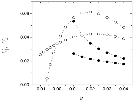
This result is in reasonable agreement with the direct measurement of Vsubscript𝑉parallel-toV_{\parallel} and Vsubscript𝑉perpendicular-toV_{\perp}, performed for the discrete model (Figures 5 and 6). From Fig. 5 we estimate V(g)V(g)αgsubscript𝑉perpendicular-to𝑔subscript𝑉parallel-to𝑔𝛼𝑔V_{\perp}(g)-V_{\parallel}(g)\approx\alpha g for small g𝑔g with α8𝛼8\alpha\approx 8, while the direct calculation from (16) using the parameters b=0.7,U=0.5,M=40formulae-sequence𝑏0.7formulae-sequence𝑈0.5𝑀40b=0.7,U=0.5,M=40, gives 3b38UM=α=10.33superscript𝑏38𝑈𝑀𝛼10.3\frac{3b^{3}}{8U}M=\alpha=10.3. From Fig. 6 we estimate α3𝛼3\alpha\approx 3  while the theoretical prediction gives α3.75𝛼3.75\alpha\approx 3.75.

Refer to caption

Figure 5: Horizontal and vertical bunch speeds V,Vsubscript𝑉parallel-tosubscript𝑉perpendicular-toV_{\parallel},V_{\perp} versus g𝑔g for the discrete model (diamonds and triangles, respectively), and for the continuous model (thick lines). Parameters are b=0.7,U=0.5,M=40formulae-sequence𝑏0.7formulae-sequence𝑈0.5𝑀40b=0.7,U=0.5,M=40.

Refer to caption

Figure 6: Horizontal and vertical bunch speeds as functions of g𝑔g for the parameters b=0.5,U=0.5formulae-sequence𝑏0.5𝑈0.5b=0.5,U=0.5 and M=40𝑀40M=40 (open circles) and M=80𝑀80M=80 (filled circles) obtained from simulations of the discrete model. Results for M=80𝑀80M=80 are reported only for large g𝑔g. In the physical region g>0𝑔0g>0, V>Vsubscript𝑉perpendicular-tosubscript𝑉parallel-toV_{\perp}>V_{\parallel}, which corresponds to step trajectories in the comoving system of coordinates going downwards (compare to Figs.7 and 8). For large g𝑔g, the absolute values and the difference V=Vsubscript𝑉perpendicular-tosubscript𝑉parallel-toV_{\perp}=V_{\parallel} are decreasing functions of M𝑀M. For small g𝑔g, VVαgsubscript𝑉perpendicular-tosubscript𝑉parallel-to𝛼𝑔V_{\perp}-V_{\parallel}\approx\alpha g where α3𝛼3\alpha\approx 3. From Eq.(16) we get the theoretical estimate α=𝛼absent\alpha= 3b38UM=3.753superscript𝑏38𝑈𝑀3.75\frac{3b^{3}}{8U}M=3.75

The result (16) is quite surprising: It tells us that the difference V(g)V(g)subscript𝑉perpendicular-to𝑔subscript𝑉parallel-to𝑔V_{\perp}(g)-V_{\parallel}(g) acquires a singularity at g=0𝑔0g=0 in the limit M𝑀M\rightarrow\infty, where continuum theory should become accurate. To avoid this unphysical singularity, we must assume the existence of an upper bound on M𝑀M (and hence, on the wavelength of moving bunch solutions) for small but positive values of g𝑔g. Indeed, in the discrete simulations to be reported in the next section, we will see that the coarsening is arrested at a certain maximum wavelength Mcrit(g)subscript𝑀𝑐𝑟𝑖𝑡𝑔M_{crit}(g). On the other hand, since in the conservative case (g=0𝑔0g=0) the vertical and horizontal excess speed of the bunch are equal, V=Vsubscript𝑉perpendicular-tosubscript𝑉parallel-toV_{\perp}=V_{\parallel}, we expect from (16) that limg0gMcrit(g)=0subscript𝑔0𝑔subscript𝑀𝑐𝑟𝑖𝑡𝑔0\lim_{g\rightarrow 0}gM_{crit}(g)=0. In other words, we deduce that for small g𝑔g the critical bunch size Mcritsubscript𝑀𝑐𝑟𝑖𝑡M_{crit} must grow more slowly than 1/g1𝑔1/g. Note also that in the conservative case the values of the excess velocities decrease with the bunch size M𝑀M as V=V3b/Msubscript𝑉perpendicular-tosubscript𝑉parallel-to3𝑏𝑀V_{\perp}=V_{\parallel}\approx 3b/M popkovkrug . We observe a similar tendency (decrease of Vsubscript𝑉perpendicular-toV_{\perp} and Vsubscript𝑉parallel-toV_{\parallel} with increasing M𝑀M) for large enough g𝑔g, compare the upper and the lower curves in Fig.6.

V Numerical simulations of the discrete equations

We simulated the coupled system (7) of M𝑀M non-linear ordinary differential equations of first order with four independent parameters: M𝑀M is the number of steps, g𝑔g is the parameter describing the non-conserving effects, b𝑏b is the parameter describing the Ehrlich-Schwoebel asymmetry and U𝑈U is the relaxation parameter due to the step-step interactions. We studied the following region of the parameter space: b[0,1]𝑏01b\in[0,1], U[0,1]𝑈01U\in[0,1], g[0,1]𝑔01g\in[0,1] and M<100𝑀100M<100. Note that, according to the definition of U𝑈U in Eq.(III.1), the dimensionless ratio gl/U=l(l+l+)/lD2𝑔𝑙𝑈𝑙subscript𝑙subscript𝑙superscriptsubscript𝑙𝐷2gl/U=l(l_{-}+l_{+})/l_{D}^{2} should be small compared to unity in order to be consistent with the assumption lDl±lmuch-greater-thansubscript𝑙𝐷subscript𝑙plus-or-minusmuch-greater-than𝑙l_{D}\gg l_{\pm}\gg l under which the model (7) was derived. Since our main interest here is in exploring the qualitative consequences of the non-conserved dynamics induced by the g𝑔g-term, rather than in a realistic description of a particular physical system, we will not always adhere to this restriction.

For the numerical integration we used an odeint-type procedure Num with periodic boundary conditions. The height of a single step and the average terrace width l𝑙l are normalized to unity. The time scale is normalized by Resubscript𝑅𝑒R_{e} and we measured the time of integration in time units (t.u.). We started with two qualitatively different initial conditions: first, an initial ’shock’ composed of densely packed steps and a very large terrace, and second, a randomly disturbed equidistant step train, where the relative amplitude of initial fluctuations is chosen to be either small (0.01) or large (0.5).

We define a bunch as a region where the widths lisubscript𝑙𝑖l_{i} of consecutive terraces are smaller than one. Figure 7a) shows a step train profile in the linear instability regime (b>6g𝑏6𝑔b>6g). As useful quantitative measures of the bunch geometry we define the maximal slope mmaxmaxi{mi}subscript𝑚𝑚𝑎𝑥subscript𝑖subscript𝑚𝑖m_{max}\equiv\max_{i}\{m_{i}\} and the minimal (=maximally negative) curvature κminmini{κi}subscript𝜅𝑚𝑖𝑛subscript𝑖subscript𝜅𝑖\kappa_{min}\equiv\min_{i}\{\kappa_{i}\}, where

mi=1li,κi=8li+1li(li+1+li)3.formulae-sequencesubscript𝑚𝑖1subscript𝑙𝑖subscript𝜅𝑖8subscript𝑙𝑖1subscript𝑙𝑖superscriptsubscript𝑙𝑖1subscript𝑙𝑖3\displaystyle m_{i}=\frac{1}{l_{i}},\ \ \ \ \ \ \ \ \ \ \ \kappa_{i}=-8\frac{l_{i+1}-l_{i}}{(l_{i+1}+l_{i})^{3}}.

We calculate and plot the positions of the steps in a co-moving coordinate system defined by x~i(t)=xi(t)ltsubscript~𝑥𝑖𝑡subscript𝑥𝑖𝑡𝑙𝑡\tilde{x}_{i}(t)=x_{i}(t)-lt, where l𝑙l is the average velocity in the conserved limit (g=0𝑔0g=0). Because of the additional nonconservative terms, there is a lateral shift after every period, see Fig. 7b) and also Fig. 8a).

For simulations with b6gless-than-or-similar-to𝑏6𝑔b\lesssim 6g an initial step bunch dissolves and approaches the configuration of equidistant steps. On the other hand for b>6g𝑏6𝑔b>6g and increasing g/U𝑔𝑈g/U, the time evolution of the step train switches unexpectedly to anti-coarsening or arrested coarsening regimes, depending on the initial conditions. In the following we describe these two scenarios in more detail.

Refer to caption
Refer to caption
Figure 7: Simulation results for M=40𝑀40M=40, b=0.1,g=0.001,U=0.004formulae-sequence𝑏0.1formulae-sequence𝑔0.001𝑈0.004b=0.1,\ g=0.001,\ U=0.004, starting with an initial shock and periodic boundary conditions. a) Typical step train profile after 1000 t.u.; b) Typical time evolution of one of the steps in co-moving coordinates.

V.1 Anti-Coarsening

Refer to caption
Refer to caption
Refer to caption
Refer to caption
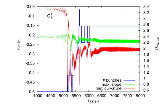
Figure 8: An example for the splitting of a large bunch in a system of 80 steps with parameters b=0.7,g=0.05,U=0.05formulae-sequence𝑏0.7formulae-sequence𝑔0.05𝑈0.05b=0.7,\ g=0.05,\ U=0.05. a) Time evolution of one of the steps. b) Plot of all step trajectories between 520052005200t.u. and 530053005300t.u. c) Comparison of the profiles after 4000 t.u., 6000 t.u., 7000 t.u. and 8000 t.u. d) (Color online) Time evolution of the globally maximal slope, the globally minimal curvature and the number of bunches.

The first surprising result we observed is the splitting of a bunch into two or more bunches after starting with an initial shock of steps. Let us consider the example in Fig. 8. The system consists of 80 steps with parameters b=0.7,g=0.05formulae-sequence𝑏0.7𝑔0.05b=0.7,\ g=0.05 andU=0.05𝑈0.05\ U=0.05. Figure 8a) shows the time evolution of the position x1subscript𝑥1x_{1} of one of the steps. There is a constant shift until the bunch splits, and then the shift increases, which corresponds to a much faster moving step. In Fig. 8b) we plot the positions of all steps around the time of the spliting, where we can see the emergence of an additional, very small but growing bunch. The splitting event is followed by another one and so forth until there are five almost equally sized bunches at 8000 t.u., see the surface height profiles in 8c). In Fig. 8d) we show the time evolution of the minimal curvature, the maximal slope and the number of bunches. In the splitting region the minimal curvature is seen to show a strong signature with an abrupt jump followed by relaxation to a smaller value, whereas the change in the maximal slope is rather small. The splitting of bunches in this system is an example of anti-coarsening, where a large structure breaks up into multiple small structures.

V.2 Arrested coarsening
Refer to caption
Refer to caption
Refer to caption
Refer to caption
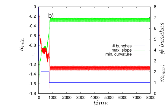
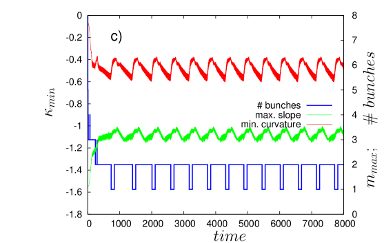
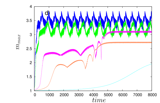
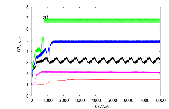
Figure 9: (Color online) An example of arrested coarsening starting with fluctuating initial conditions of strong amplitude, for M=40𝑀40M=40 and U=0.2𝑈0.2U=0.2. a) Maximal slope for b=0.7𝑏0.7b=0.7 and (from top to bottom) g=0, 0.01, 0.02, 0.05, 0.09𝑔00.010.020.050.09g=0,\ 0.01,\ 0.02,\ 0.05,\ 0.09. b) Number of bunches, maximal slope and minimal curvature for b=0.7𝑏0.7b=0.7 and g=0𝑔0g=0. c) As b) for b=0.7𝑏0.7b=0.7 and g=0.02𝑔0.02g=0.02; d) Maximal slope for g=0.02𝑔0.02g=0.02 and (from top to bottom) b=0.9, 0.7, 0.4, 0.3, 0.2𝑏0.90.70.40.30.2b=0.9,\ 0.7,\ 0.4,\ 0.3,\ 0.2.

The second type of initial condition is a randomly perturbed equidistant step train. As an example, see Fig. 9, we take M=40𝑀40M=40, U=0.2𝑈0.2U=0.2, a strong perturbation amplitude, an integration time of 8000 t.u., and vary the parameters g𝑔g and b𝑏b. We use the time evolution of the global maximal slope mmax(t)subscript𝑚𝑚𝑎𝑥𝑡m_{max}(t) in order to identify the final state of the simulation. As can be seen in Fig. 9a), after about 2000 t.u. the simulations settled down into a periodic attractor of varying complexity. In Fig. 9b) we show the case of vanishing g𝑔g, which corresponds to a conventional coarsening behavior: After a short time the number of bunches goes to unity and mmaxsubscript𝑚𝑚𝑎𝑥m_{max} and κminsubscript𝜅𝑚𝑖𝑛\kappa_{min} vary periodically on the characteristic time scale in which the bunch profile shifts by one average terrace size popkovkrug . By increasing g𝑔g a point is reached where coarsening into a single bunch no longer occurs, see Fig. 9c). The system is now jumping periodically between configurations with two bunches and one bunch. Upon further increasing g𝑔g the period of the jumps diverges and the stable state becomes a configuration of two bunches. Finally, Fig. 9d) displays the various regimes of temporal behavior that occur when varying b𝑏b at fixed g𝑔g.

Refer to caption
Refer to caption
Figure 10: Stability/instability diagrams showing the number of bunches in the final state, for M=40𝑀40M=40 and different combinations of b𝑏b and g𝑔g. a) U=0.2𝑈0.2U=0.2; b) U=0.05𝑈0.05U=0.05 - \blacktriangle: region depending sensitive on the initial condition, \square: 1 bunch, \bullet: 1/2 bunches, ×\times: 2 bunches, \triangle: 2/3 bunches, \blacksquare: 3 bunches, ++: 3/4 bunches, \circ: 4 bunches, below the line b=6g𝑏6𝑔b=6g: stability

V.3 Phase diagrams

To somewhat systemize these observations, in Fig. 10 we present two phase diagram where the number of bunches is shown in the (g,b)𝑔𝑏(g,b)-plane for b[0,1]𝑏01b\in[0,1] with increments of b=0.1𝑏0.1\triangle b=0.1 and g[0,0.1]𝑔00.1g\in[0,0.1] with increments of g=0.01𝑔0.01\triangle g=0.01. For U=0.2𝑈0.2U=0.2 [Fig. 10a)] the number of bunches in the final stationary state is between one and two. At g=0.02𝑔0.02g=0.02, b=0.4𝑏0.4b=0.4 the relaxation time is very sensitive to the initial random configuration and one needs more than 8000 t.u. to switch to the single bunch configuration; moreover, around this point the final state depends sensitively on initial conditions. For U=0.05𝑈0.05U=0.05 the number of bunches changes between 4 and an oscillatory state with 1-2 bunches, but a stable state with a single bunch is not seen. In general, we observe that the smaller U𝑈U the larger is the possible number of bunches. For example for U=0𝑈0U=0, M=40𝑀40M=40, g=0.02𝑔0.02g=0.02 and b=0.5𝑏0.5b=0.5, there are 18 bunches in the final state, corresponding to less than 2.5 steps pro bunch.
Refer to caption
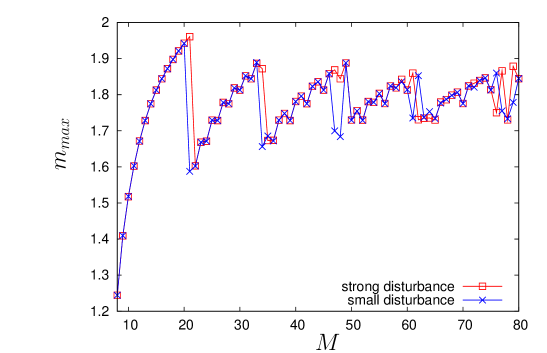
Figure 11: (Color online) Dependence of the upper boundary of the globally maximal slope mmaxsubscript𝑚𝑚𝑎𝑥m_{max} on the number of steps M𝑀M for g=U=0.04𝑔𝑈0.04g=U=0.04, b=0.4𝑏0.4b=0.4 and for large and small amplitude of the initial random condition.

In Fig. 11 we show the dependence of the globally maximal slope mmaxsubscript𝑚𝑚𝑎𝑥m_{max} on M𝑀M for g=U=0.04𝑔𝑈0.04g=U=0.04 and b=0.4𝑏0.4b=0.4. As we have seen in Fig.9, mmaxsubscript𝑚𝑚𝑎𝑥m_{max} generally oscillates in the final state. In order to uniquely define mmaxsubscript𝑚𝑚𝑎𝑥m_{max} we take for reference its largest value during the last 500 t.u. of the simulation. For a strong initial disturbance mmaxsubscript𝑚𝑚𝑎𝑥m_{max} grows up to 1.96 at M=21𝑀21M=21 steps and then jumps down to 1.60 at M=22𝑀22M=22, where the step train switches from a single bunch to a configuration with two bunches; for a weak initial disturbance the behavior is similar but the jump occurs slightly earlier. With increasing M𝑀M this behavior repeats several times until in the region of 80 steps the switching becomes less regular and depends strongly on the initial disturbance. The overall pattern in Fig.11 suggests that the splitting of bunches is driven by the tendency of the system to keep the maximal slope below a certain limiting value, thus connecting the behavior of the discrete system to the properties of stationary solutions of the continuum equation discussed in Sect.IV.

VI Summary and discussion

In this paper we have investigated the extension (7) of a previously studied, minimal model of step bunching during sublimation. Despite the smallness of the dimensionless coefficient g𝑔g describing the interplay between sublimation and capillarity, the non-conservative nature of the dynamics was found to have profound effects on the linear as well as on the nonlinear level. In order to analytically study the nonlinear behavior of step bunches, we derived and analyzed the continuum evolution equation (10) for the surface profile. Using two different types of approximations, we deduced that the non-conservative terms in this equation place an upper limit on the slope as well as on the wavelength of step bunches. This conclusion was confirmed by a detailed numerical study of the discrete step dynamics, which also revealed additional complex dynamical regimes in which the number of step bunches increases in time or oscillates between different values.

To place our findings into context, we note that a connection between unbounded coarsening of step bunches and the conservative nature of the dynamics has been observed in previous work. First, Sato and Uwaha studied step bunching induced by electromigration and observed a saturation of the mean bunch size when sublimation was included Sato1999 . A direct comparison to our results is difficult, however, since they use a different set of step dynamical equations which depend on a larger set of parameters.

Second, the difference between conserved and non-conserved surface dynamics has been addressed in the framework of weakly nonlinear (in the sense of PierreLouis2005b ) continuum equations. Working close to the instability threshold, Sato and Uwaha Sato1995 and Misbah and Pierre-Louis Misbah1996 showed that the large-scale dynamics of step bunches in a non-conserved setting is described by the Benney equation. Depending on the size of a term that breaks the left-right symmetry, this equation displays either spatio-temporal chaos or an ordered array of bunches, but no coarsening. On the other hand, the corresponding conservative equation derived in Gillet2001 does show unlimited coarsening with the average bunch size growing as t1/2superscript𝑡12t^{1/2}. In general, deducing the coarsening behavior of a given nonlinear evolution equation by analytic means is a difficult problem, and the methods available so far Politi2006 do not seem to readily carry over to highly nonlinear equations like (10).

Acknowledgements

We thank P. Politi, B. Ranguelov, S. Stoyanov and V. Tonchev for useful discussions.

Appendix A Discrete equations for the case of sublimation

A.1 The concentration profile

In the quasistatic approximation ni/t=0subscript𝑛𝑖𝑡0\partial n_{i}/\partial t=0 (1) with F=0𝐹0F=0 is a homogeneous ordinary differential equation of second order with the following general solution:

ni(x)=C1iexlD+C2iexlD.subscript𝑛𝑖𝑥superscriptsubscript𝐶1𝑖superscript𝑒𝑥subscript𝑙𝐷superscriptsubscript𝐶2𝑖superscript𝑒𝑥subscript𝑙𝐷n_{i}(x)=C_{1}^{i}e^{\frac{x}{l_{D}}}+C_{2}^{i}e^{-\frac{x}{l_{D}}}. (17)

In order to find the constants of integration C1isuperscriptsubscript𝐶1𝑖C_{1}^{i} and C2isuperscriptsubscript𝐶2𝑖C_{2}^{i} we use the boundary conditions (II):

Dsk(C1ilDeli2lDC2ilDe+li2lD)subscript𝐷𝑠subscript𝑘superscriptsubscript𝐶1𝑖subscript𝑙𝐷superscript𝑒subscript𝑙𝑖2subscript𝑙𝐷superscriptsubscript𝐶2𝑖subscript𝑙𝐷superscript𝑒subscript𝑙𝑖2subscript𝑙𝐷\displaystyle\frac{D_{s}}{k_{-}}\left(\frac{C_{1}^{i}}{l_{D}}e^{-\frac{l_{i}}{2l_{D}}}-\frac{C_{2}^{i}}{l_{D}}e^{+\frac{l_{i}}{2l_{D}}}\right) =\displaystyle= +C1ieli2lD+C2ie+li2lDneq0(1+μikT),superscriptsubscript𝐶1𝑖superscript𝑒subscript𝑙𝑖2subscript𝑙𝐷superscriptsubscript𝐶2𝑖superscript𝑒subscript𝑙𝑖2subscript𝑙𝐷subscriptsuperscript𝑛0𝑒𝑞1subscript𝜇𝑖𝑘𝑇\displaystyle+C_{1}^{i}e^{-\frac{l_{i}}{2l_{D}}}+C_{2}^{i}e^{+\frac{l_{i}}{2l_{D}}}-n^{0}_{eq}\left(1+\frac{\mu_{i}}{kT}\right),
Dsk+(C1ilDe+li2lDC2ilDeli2lD)subscript𝐷𝑠subscript𝑘superscriptsubscript𝐶1𝑖subscript𝑙𝐷superscript𝑒subscript𝑙𝑖2subscript𝑙𝐷superscriptsubscript𝐶2𝑖subscript𝑙𝐷superscript𝑒subscript𝑙𝑖2subscript𝑙𝐷\displaystyle\frac{D_{s}}{k_{+}}\left(\frac{C_{1}^{i}}{l_{D}}e^{+\frac{l_{i}}{2l_{D}}}-\frac{C_{2}^{i}}{l_{D}}e^{-\frac{l_{i}}{2l_{D}}}\right) =\displaystyle= C1ie+li2lDC2ieli2lD+neq0(1+μi+1kT).superscriptsubscript𝐶1𝑖superscript𝑒subscript𝑙𝑖2subscript𝑙𝐷superscriptsubscript𝐶2𝑖superscript𝑒subscript𝑙𝑖2subscript𝑙𝐷subscriptsuperscript𝑛0𝑒𝑞1subscript𝜇𝑖1𝑘𝑇\displaystyle-C_{1}^{i}e^{+\frac{l_{i}}{2l_{D}}}-C_{2}^{i}e^{-\frac{l_{i}}{2l_{D}}}+n^{0}_{eq}\left(1+\frac{\mu_{i+1}}{kT}\right).

Substituting l±:=DslDk±=l±lDassignsuperscript𝑙plus-or-minussubscript𝐷𝑠subscript𝑙𝐷subscript𝑘plus-or-minussubscript𝑙plus-or-minussubscript𝑙𝐷l^{\pm}:=\frac{D_{s}}{l_{D}k_{\pm}}=\frac{l_{\pm}}{l_{D}} this becomes

(l1)C1ieli2lD(l+1)C2ie+li2lDsuperscript𝑙1superscriptsubscript𝐶1𝑖superscript𝑒subscript𝑙𝑖2subscript𝑙𝐷superscript𝑙1superscriptsubscript𝐶2𝑖superscript𝑒subscript𝑙𝑖2subscript𝑙𝐷\displaystyle(l^{-}-1)C_{1}^{i}e^{-\frac{l_{i}}{2l_{D}}}-(l^{-}+1)C_{2}^{i}e^{+\frac{l_{i}}{2l_{D}}} =\displaystyle= neq0(1+μikT),subscriptsuperscript𝑛0𝑒𝑞1subscript𝜇𝑖𝑘𝑇\displaystyle-n^{0}_{eq}\left(1+\frac{\mu_{i}}{kT}\right),
(l++1)C1ie+li2lD(l+1)C2ieli2lDsuperscript𝑙1superscriptsubscript𝐶1𝑖superscript𝑒subscript𝑙𝑖2subscript𝑙𝐷superscript𝑙1superscriptsubscript𝐶2𝑖superscript𝑒subscript𝑙𝑖2subscript𝑙𝐷\displaystyle(l^{+}+1)C_{1}^{i}e^{+\frac{l_{i}}{2l_{D}}}-(l^{+}-1)C_{2}^{i}e^{-\frac{l_{i}}{2l_{D}}} =\displaystyle= +neq0(1+μi+1kT).subscriptsuperscript𝑛0𝑒𝑞1subscript𝜇𝑖1𝑘𝑇\displaystyle+n^{0}_{eq}\left(1+\frac{\mu_{i+1}}{kT}\right).

After adding both equations and solving for C1isuperscriptsubscript𝐶1𝑖C_{1}^{i} we obtain

C1i=neq0(μi+1kTμikT)+C2i[(l+1)eli2lD+(l+1)eli2lD](l1)eli2lD+(l++1)eli2lD.superscriptsubscript𝐶1𝑖subscriptsuperscript𝑛0𝑒𝑞subscript𝜇𝑖1𝑘𝑇subscript𝜇𝑖𝑘𝑇superscriptsubscript𝐶2𝑖delimited-[]superscript𝑙1superscript𝑒subscript𝑙𝑖2subscript𝑙𝐷superscript𝑙1superscript𝑒subscript𝑙𝑖2subscript𝑙𝐷superscript𝑙1superscript𝑒subscript𝑙𝑖2subscript𝑙𝐷superscript𝑙1superscript𝑒subscript𝑙𝑖2subscript𝑙𝐷\displaystyle C_{1}^{i}=\frac{n^{0}_{eq}\left(\frac{\mu_{i+1}}{kT}-\frac{\mu_{i}}{kT}\right)+C_{2}^{i}\left[\left(l^{-}+1\right)e^{\frac{l_{i}}{2l_{D}}}+\left(l^{+}-1\right)e^{-\frac{l_{i}}{2l_{D}}}\right]}{\left(l^{-}-1\right)e^{-\frac{l_{i}}{2l_{D}}}+\left(l^{+}+1\right)e^{\frac{l_{i}}{2l_{D}}}}. (18)

We substitute C1isuperscriptsubscript𝐶1𝑖C_{1}^{i} in the first boundary condition:

C2i=neq0(1+μikT)+C1i(l1)eλ1li2(l+1)eλ2li2.superscriptsubscript𝐶2𝑖subscriptsuperscript𝑛0𝑒𝑞1subscript𝜇𝑖𝑘𝑇superscriptsubscript𝐶1𝑖superscript𝑙1superscript𝑒subscript𝜆1subscript𝑙𝑖2superscript𝑙1superscript𝑒subscript𝜆2subscript𝑙𝑖2\displaystyle C_{2}^{i}=\frac{n^{0}_{eq}\left(1+\frac{\mu_{i}}{kT}\right)+C_{1}^{i}(l^{-}-1)e^{-\lambda_{1}\frac{l_{i}}{2}}}{(l^{-}+1)e^{-\lambda_{2}\frac{l_{i}}{2}}}. (19)

After back substitution from C2isuperscriptsubscript𝐶2𝑖C_{2}^{i} into C1isuperscriptsubscript𝐶1𝑖C_{1}^{i} and vice versa we get the final form for the constants:

C1isuperscriptsubscript𝐶1𝑖\displaystyle C_{1}^{i} =\displaystyle= neq02[(l+1)(1+μikT)eli2lD+(l+1)(1+μi+1kT)eli2lD(l+l+1)sinhlilD+(l+l+)coshlilD],subscriptsuperscript𝑛0𝑒𝑞2delimited-[]superscript𝑙11subscript𝜇𝑖𝑘𝑇superscript𝑒subscript𝑙𝑖2subscript𝑙𝐷superscript𝑙11subscript𝜇𝑖1𝑘𝑇superscript𝑒subscript𝑙𝑖2subscript𝑙𝐷superscript𝑙superscript𝑙1subscript𝑙𝑖subscript𝑙𝐷superscript𝑙superscript𝑙subscript𝑙𝑖subscript𝑙𝐷\displaystyle\frac{n^{0}_{eq}}{2}\left[\frac{(l^{+}-1)(1+\frac{\mu_{i}}{kT})e^{-\frac{l_{i}}{2l_{D}}}+(l^{-}+1)(1+\frac{\mu_{i+1}}{kT})e^{\frac{l_{i}}{2l_{D}}}}{(l^{+}l^{-}+1)\sinh\frac{l_{i}}{l_{D}}+(l^{-}+l^{+})\cosh\frac{l_{i}}{l_{D}}}\right],
C2isuperscriptsubscript𝐶2𝑖\displaystyle C_{2}^{i} =\displaystyle= neq02[(l1)(1+μikT)eli2lD+(l++1)(1+μi+1kT)eli2lD(l+l+1)sinhlilD+(l+l+)coshlilD].subscriptsuperscript𝑛0𝑒𝑞2delimited-[]superscript𝑙11subscript𝜇𝑖𝑘𝑇superscript𝑒subscript𝑙𝑖2subscript𝑙𝐷superscript𝑙11subscript𝜇𝑖1𝑘𝑇superscript𝑒subscript𝑙𝑖2subscript𝑙𝐷superscript𝑙superscript𝑙1subscript𝑙𝑖subscript𝑙𝐷superscript𝑙superscript𝑙subscript𝑙𝑖subscript𝑙𝐷\displaystyle\frac{n^{0}_{eq}}{2}\left[\frac{(l^{-}-1)(1+\frac{\mu_{i}}{kT})e^{-\frac{l_{i}}{2l_{D}}}+(l^{+}+1)(1+\frac{\mu_{i+1}}{kT})e^{\frac{l_{i}}{2l_{D}}}}{(l^{+}l^{-}+1)\sinh\frac{l_{i}}{l_{D}}+(l^{-}+l^{+})\cosh\frac{l_{i}}{l_{D}}}\right]. (20)

A.2 Fluxes and the step velocities

Using the definition

f±i(x)=±ΩDsni(x)xatx=±li2formulae-sequencesubscriptsuperscript𝑓𝑖plus-or-minus𝑥plus-or-minusΩsubscript𝐷𝑠subscript𝑛𝑖𝑥𝑥at𝑥plus-or-minussubscript𝑙𝑖2f^{i}_{\pm}(x)=\pm\Omega D_{s}\frac{\partial n_{i}(x)}{\partial x}\ \ \text{at}\ x=\pm\frac{l_{i}}{2}

we find for the fluxes to the step bordering the i𝑖ith terrace of width lisubscript𝑙𝑖l_{i}:

f+isuperscriptsubscript𝑓𝑖\displaystyle f_{+}^{i} =\displaystyle= ΩDsneq0lD(1+μi+1kT)(lsinhlilD+coshlilD)(1+μikT)(l+l+1)sinhlilD+(l+l+)coshlilD,at stepi+1,Ωsubscript𝐷𝑠subscriptsuperscript𝑛0𝑒𝑞subscript𝑙𝐷1subscript𝜇𝑖1𝑘𝑇superscript𝑙subscript𝑙𝑖subscript𝑙𝐷subscript𝑙𝑖subscript𝑙𝐷1subscript𝜇𝑖𝑘𝑇superscript𝑙superscript𝑙1subscript𝑙𝑖subscript𝑙𝐷superscript𝑙superscript𝑙subscript𝑙𝑖subscript𝑙𝐷at step𝑖1\displaystyle\frac{\Omega D_{s}n^{0}_{eq}}{l_{D}}\frac{\left(1+\frac{\mu_{i+1}}{kT}\right)\left(l^{-}\sinh\frac{l_{i}}{l_{D}}+\cosh\frac{l_{i}}{l_{D}}\right)-\left(1+\frac{\mu_{i}}{kT}\right)}{(l^{+}l^{-}+1)\sinh\frac{l_{i}}{l_{D}}+(l^{-}+l^{+})\cosh\frac{l_{i}}{l_{D}}},\ \ \text{at step}\ i+1,
fisuperscriptsubscript𝑓𝑖\displaystyle f_{-}^{i} =\displaystyle= ΩDsneq0lD(1+μikT)(l+sinhlilD+coshlilD)(1+μi+1kT)(l+l+1)sinhlilD+(l+l+)coshlilD,at stepi.Ωsubscript𝐷𝑠subscriptsuperscript𝑛0𝑒𝑞subscript𝑙𝐷1subscript𝜇𝑖𝑘𝑇superscript𝑙subscript𝑙𝑖subscript𝑙𝐷subscript𝑙𝑖subscript𝑙𝐷1subscript𝜇𝑖1𝑘𝑇superscript𝑙superscript𝑙1subscript𝑙𝑖subscript𝑙𝐷superscript𝑙superscript𝑙subscript𝑙𝑖subscript𝑙𝐷at step𝑖\displaystyle\frac{\Omega D_{s}n^{0}_{eq}}{l_{D}}\frac{\left(1+\frac{\mu_{i}}{kT}\right)\left(l^{+}\sinh\frac{l_{i}}{l_{D}}+\cosh\frac{l_{i}}{l_{D}}\right)-\left(1+\frac{\mu_{i+1}}{kT}\right)}{(l^{+}l^{-}+1)\sinh\frac{l_{i}}{l_{D}}+(l^{-}+l^{+})\cosh\frac{l_{i}}{l_{D}}},\ \ \text{at step}\ i.

Adding the fluxes from the two neighboring terraces we obtain the expression for the velocity of step i𝑖i as vi=dxidt=fi+f+i1subscript𝑣𝑖𝑑subscript𝑥𝑖𝑑𝑡superscriptsubscript𝑓𝑖superscriptsubscript𝑓𝑖1v_{i}=\frac{dx_{i}}{dt}=f_{-}^{i}+f_{+}^{i-1}.

A.3 Linear stability analysis

Let us assume that lDlmuch-greater-thansubscript𝑙𝐷𝑙l_{D}\gg l and lDl±much-greater-thansubscript𝑙𝐷subscript𝑙plus-or-minusl_{D}\gg l_{\pm}. Then sinhlilDlilDsubscript𝑙𝑖subscript𝑙𝐷subscript𝑙𝑖subscript𝑙𝐷\sinh\frac{l_{i}}{l_{D}}\approx\frac{l_{i}}{l_{D}} and coshlilD1.subscript𝑙𝑖subscript𝑙𝐷1\cosh\frac{l_{i}}{l_{D}}\approx 1. For the denominator in the expression for the fluxes (and with l±=l±lDsuperscript𝑙plus-or-minussubscript𝑙plus-or-minussubscript𝑙𝐷l^{\pm}=\frac{l_{\pm}}{l_{D}}) we find

(l+llD2+1)sinhlilD+(llD+l+lD)coshlilDsubscript𝑙subscript𝑙superscriptsubscript𝑙𝐷21subscript𝑙𝑖subscript𝑙𝐷subscript𝑙subscript𝑙𝐷subscript𝑙subscript𝑙𝐷subscript𝑙𝑖subscript𝑙𝐷\displaystyle(\frac{l_{+}l_{-}}{l_{D}^{2}}+1)\sinh\frac{l_{i}}{l_{D}}+(\frac{l_{-}}{l_{D}}+\frac{l_{+}}{l_{D}})\cosh\frac{l_{i}}{l_{D}} \displaystyle\approx l+l++lilD,subscript𝑙subscript𝑙subscript𝑙𝑖subscript𝑙𝐷\displaystyle\frac{l_{-}+l_{+}+l_{i}}{l_{D}}, (21)

and the velocity becomes

1ΩDsneq0dxidt1Ωsubscript𝐷𝑠subscriptsuperscript𝑛0𝑒𝑞𝑑subscript𝑥𝑖𝑑𝑡\displaystyle\frac{1}{\Omega D_{s}n^{0}_{eq}}\frac{dx_{i}}{dt} \displaystyle\approx (1+μikT)(lli1lD2+1)(1+μi1kT)l+l++li1+(1+μikT)(l+lilD2+1)(1+μi+1kT)l+l++li1subscript𝜇𝑖𝑘𝑇subscript𝑙subscript𝑙𝑖1subscriptsuperscript𝑙2𝐷11subscript𝜇𝑖1𝑘𝑇subscript𝑙subscript𝑙subscript𝑙𝑖11subscript𝜇𝑖𝑘𝑇subscript𝑙subscript𝑙𝑖subscriptsuperscript𝑙2𝐷11subscript𝜇𝑖1𝑘𝑇subscript𝑙subscript𝑙subscript𝑙𝑖\displaystyle\frac{\left(1+\frac{\mu_{i}}{kT}\right)\left(\frac{l_{-}l_{i-1}}{l^{2}_{D}}+1\right)-\left(1+\frac{\mu_{i-1}}{kT}\right)}{l_{-}+l_{+}+l_{i-1}}+\frac{\left(1+\frac{\mu_{i}}{kT}\right)\left(\frac{l_{+}l_{i}}{l^{2}_{D}}+1\right)-\left(1+\frac{\mu_{i+1}}{kT}\right)}{l_{-}+l_{+}+l_{i}} (22)
=\displaystyle= (1+μikT)lli1lD2+(μikTμi1kT)l+l++li1+(1+μikT)l+lilD2+(μikTμi+1kT)l+l++li1subscript𝜇𝑖𝑘𝑇subscript𝑙subscript𝑙𝑖1subscriptsuperscript𝑙2𝐷subscript𝜇𝑖𝑘𝑇subscript𝜇𝑖1𝑘𝑇subscript𝑙subscript𝑙subscript𝑙𝑖11subscript𝜇𝑖𝑘𝑇subscript𝑙subscript𝑙𝑖subscriptsuperscript𝑙2𝐷subscript𝜇𝑖𝑘𝑇subscript𝜇𝑖1𝑘𝑇subscript𝑙subscript𝑙subscript𝑙𝑖\displaystyle\frac{\left(1+\frac{\mu_{i}}{kT}\right)\frac{l_{-}l_{i-1}}{l^{2}_{D}}+(\frac{\mu_{i}}{kT}-\frac{\mu_{i-1}}{kT})}{l_{-}+l_{+}+l_{i-1}}+\frac{\left(1+\frac{\mu_{i}}{kT}\right)\frac{l_{+}l_{i}}{l^{2}_{D}}+(\frac{\mu_{i}}{kT}-\frac{\mu_{i+1}}{kT})}{l_{-}+l_{+}+l_{i}}

The chemical potential μisubscript𝜇𝑖\mu_{i} can be linearized as

μikTg[13εi+1εil1+3εiεi1l]=3gl(2εiεi+1εi1)subscript𝜇𝑖𝑘𝑇𝑔delimited-[]13subscript𝜀𝑖1subscript𝜀𝑖𝑙13subscript𝜀𝑖subscript𝜀𝑖1𝑙3𝑔𝑙2subscript𝜀𝑖subscript𝜀𝑖1subscript𝜀𝑖1absent\displaystyle\frac{\mu_{i}}{kT}\approx-g\left[1-3\frac{\varepsilon_{i+1}-\varepsilon_{i}}{l}-1+3\frac{\varepsilon_{i}-\varepsilon_{i-1}}{l}\right]=-\frac{3g}{l}(2\varepsilon_{i}-\varepsilon_{i+1}-\varepsilon_{i-1})\Rightarrow
μikTμi±1kTsubscript𝜇𝑖𝑘𝑇subscript𝜇plus-or-minus𝑖1𝑘𝑇\displaystyle\frac{\mu_{i}}{kT}-\frac{\mu_{i\pm 1}}{kT} \displaystyle\approx 3gl(3εi±1+3εi+εi±2εi1)3𝑔𝑙3subscript𝜀plus-or-minus𝑖13subscript𝜀𝑖subscript𝜀plus-or-minus𝑖2subscript𝜀minus-or-plus𝑖1\displaystyle-\frac{3g}{l}(-3\varepsilon_{i\pm 1}+3\varepsilon_{i}+\varepsilon_{i\pm 2}-\varepsilon_{i\mp 1})
(1+μikT)l±li,i1lD21subscript𝜇𝑖𝑘𝑇subscript𝑙plus-or-minussubscript𝑙𝑖𝑖1subscriptsuperscript𝑙2𝐷\displaystyle\left(1+\frac{\mu_{i}}{kT}\right)\frac{l_{\pm}l_{i,i-1}}{l^{2}_{D}} \displaystyle\approx l±lD2(l+εi+1,iεi,i1)3gl±lD2(2εiεi+1εi1)subscript𝑙plus-or-minussubscriptsuperscript𝑙2𝐷𝑙subscript𝜀𝑖1𝑖subscript𝜀𝑖𝑖13𝑔subscript𝑙plus-or-minussubscriptsuperscript𝑙2𝐷2subscript𝜀𝑖subscript𝜀𝑖1subscript𝜀𝑖1\displaystyle\frac{l_{\pm}}{l^{2}_{D}}(l+\varepsilon_{i+1,i}-\varepsilon_{i,i-1})-\frac{3gl_{\pm}}{l^{2}_{D}}(2\varepsilon_{i}-\varepsilon_{i+1}-\varepsilon_{i-1})
1ΩDsneq0dxidt1Ωsubscript𝐷𝑠subscriptsuperscript𝑛0𝑒𝑞𝑑subscript𝑥𝑖𝑑𝑡\displaystyle\frac{1}{\Omega D_{s}n^{0}_{eq}}\frac{dx_{i}}{dt} \displaystyle\approx (l++l)l(l+l++l)lD2+3g(l+l++l)l(6εi+4εi+1+4εi1εi+2εi2)subscript𝑙subscript𝑙𝑙subscript𝑙subscript𝑙𝑙subscriptsuperscript𝑙2𝐷3𝑔subscript𝑙subscript𝑙𝑙𝑙6subscript𝜀𝑖4subscript𝜀𝑖14subscript𝜀𝑖1subscript𝜀𝑖2subscript𝜀𝑖2\displaystyle\frac{(l_{+}+l_{-})l}{(l_{-}+l_{+}+l)l^{2}_{D}}+\frac{3g}{(l_{-}+l_{+}+l)l}(-6\varepsilon_{i}+4\varepsilon_{i+1}+4\varepsilon_{i-1}-\varepsilon_{i+2}-\varepsilon_{i-2}) (23)
+\displaystyle+ l(εiεi1)+l+(εi+1εi)(l+l++l)lD23g(l++l)(l+l++l)lD2(2εiεi+1+εi1)subscript𝑙subscript𝜀𝑖subscript𝜀𝑖1subscript𝑙subscript𝜀𝑖1subscript𝜀𝑖subscript𝑙subscript𝑙𝑙subscriptsuperscript𝑙2𝐷3𝑔subscript𝑙subscript𝑙subscript𝑙subscript𝑙𝑙subscriptsuperscript𝑙2𝐷2subscript𝜀𝑖subscript𝜀𝑖1subscript𝜀𝑖1\displaystyle\frac{l_{-}(\varepsilon_{i}-\varepsilon_{i-1})+l_{+}(\varepsilon_{i+1}-\varepsilon_{i})}{(l_{-}+l_{+}+l)l^{2}_{D}}-\frac{3g(l_{+}+l_{-})}{(l_{-}+l_{+}+l)l^{2}_{D}}(2\varepsilon_{i}-\varepsilon_{i+1}+\varepsilon_{i-1})
approaches-limit\displaystyle\doteq 1ΩDneq0(veq+dεidt)1Ω𝐷subscriptsuperscript𝑛0𝑒𝑞subscript𝑣𝑒𝑞𝑑subscript𝜀𝑖𝑑𝑡\displaystyle\frac{1}{\Omega Dn^{0}_{eq}}\left(v_{eq}+\frac{d\varepsilon_{i}}{dt}\right)

The equation for the perturbation reads

1ΩDsneq0dεidt1Ωsubscript𝐷𝑠subscriptsuperscript𝑛0𝑒𝑞𝑑subscript𝜀𝑖𝑑𝑡\displaystyle\frac{1}{\Omega D_{s}n^{0}_{eq}}\frac{d\varepsilon_{i}}{dt} =\displaystyle= 3g(l+l++l)l(6εi+4εi+1+4εi1εi+2εi2)3𝑔subscript𝑙subscript𝑙𝑙𝑙6subscript𝜀𝑖4subscript𝜀𝑖14subscript𝜀𝑖1subscript𝜀𝑖2subscript𝜀𝑖2\displaystyle\frac{3g}{(l_{-}+l_{+}+l)l}(-6\varepsilon_{i}+4\varepsilon_{i+1}+4\varepsilon_{i-1}-\varepsilon_{i+2}-\varepsilon_{i-2})
+\displaystyle+ l(εiεi1)+l+(εi+1εi)(l+l++l)lD23g(l++l)(l+l++l)lD2(2εiεi+1+εi1)subscript𝑙subscript𝜀𝑖subscript𝜀𝑖1subscript𝑙subscript𝜀𝑖1subscript𝜀𝑖subscript𝑙subscript𝑙𝑙subscriptsuperscript𝑙2𝐷3𝑔subscript𝑙subscript𝑙subscript𝑙subscript𝑙𝑙subscriptsuperscript𝑙2𝐷2subscript𝜀𝑖subscript𝜀𝑖1subscript𝜀𝑖1\displaystyle\frac{l_{-}(\varepsilon_{i}-\varepsilon_{i-1})+l_{+}(\varepsilon_{i+1}-\varepsilon_{i})}{(l_{-}+l_{+}+l)l^{2}_{D}}-\frac{3g(l_{+}+l_{-})}{(l_{-}+l_{+}+l)l^{2}_{D}}(2\varepsilon_{i}-\varepsilon_{i+1}+\varepsilon_{i-1})

Using the Fourier expression ε=ε0eikn+ω(k)t𝜀subscript𝜀0superscript𝑒𝑖𝑘𝑛𝜔𝑘𝑡\varepsilon=\varepsilon_{0}e^{ikn+\omega(k)t} we find the dispersion relation ω(k)𝜔𝑘\omega(k):

ω(k)ΩDsneq0𝜔𝑘Ωsubscript𝐷𝑠subscriptsuperscript𝑛0𝑒𝑞\displaystyle\frac{\omega(k)}{\Omega D_{s}n^{0}_{eq}} =\displaystyle= 3g(l+l++l)l[6+4(eik+eik)(ei2k+ei2k)]3𝑔subscript𝑙subscript𝑙𝑙𝑙delimited-[]64superscript𝑒𝑖𝑘superscript𝑒𝑖𝑘superscript𝑒𝑖2𝑘superscript𝑒𝑖2𝑘\displaystyle\frac{3g}{(l_{-}+l_{+}+l)l}[-6+4(e^{ik}+e^{-ik})-(e^{i2k}+e^{-i2k})]
+\displaystyle+ l(1eik)+l+(eik1)(l+l++l)lD23g(l++l)(l+l++l)lD2(2(eik+eik)).subscript𝑙1superscript𝑒𝑖𝑘subscript𝑙superscript𝑒𝑖𝑘1subscript𝑙subscript𝑙𝑙subscriptsuperscript𝑙2𝐷3𝑔subscript𝑙subscript𝑙subscript𝑙subscript𝑙𝑙subscriptsuperscript𝑙2𝐷2superscript𝑒𝑖𝑘superscript𝑒𝑖𝑘\displaystyle\frac{l_{-}(1-e^{-ik})+l_{+}(e^{ik}-1)}{(l_{-}+l_{+}+l)l^{2}_{D}}-\frac{3g(l_{+}+l_{-})}{(l_{-}+l_{+}+l)l^{2}_{D}}(2-(e^{ik}+e^{-ik})).

For small k𝑘k we can expand the exponential functions as

2(eik+eik)2superscript𝑒𝑖𝑘superscript𝑒𝑖𝑘\displaystyle 2-(e^{ik}+e^{-ik}) =\displaystyle= 2(1cosk)2(11+k22)=k2,21𝑘211superscript𝑘22superscript𝑘2\displaystyle 2(1-\cos k)\approx 2(1-1+\frac{k^{2}}{2})=k^{2},
64(eik+eik)+(ei2k+ei2k)64superscript𝑒𝑖𝑘superscript𝑒𝑖𝑘superscript𝑒𝑖2𝑘superscript𝑒𝑖2𝑘\displaystyle 6-4(e^{ik}+e^{-ik})+(e^{i2k}+e^{-i2k}) =\displaystyle= 4(cosk1)2k4,4superscript𝑘12superscript𝑘4\displaystyle 4(\cos k-1)^{2}\approx k^{4},
1eik1superscript𝑒𝑖𝑘\displaystyle 1-e^{-ik} \displaystyle\approx 1(1ik+k22)=ik+k22,11𝑖𝑘superscript𝑘22𝑖𝑘superscript𝑘22\displaystyle 1-(1-ik+\frac{k^{2}}{2})=ik+\frac{k^{2}}{2},

which yields an expression for the real part Re[ω]𝑅𝑒delimited-[]𝜔Re[\omega]:

Re[ω]=ΩDsneq0lD2(l+l+)(l+l++l)[(ll+)23g]k2ΩDsneq03g(l+l++l)lk4.𝑅𝑒delimited-[]𝜔Ωsubscript𝐷𝑠subscriptsuperscript𝑛0𝑒𝑞subscriptsuperscript𝑙2𝐷subscript𝑙subscript𝑙subscript𝑙subscript𝑙𝑙delimited-[]subscript𝑙subscript𝑙23𝑔superscript𝑘2Ωsubscript𝐷𝑠subscriptsuperscript𝑛0𝑒𝑞3𝑔subscript𝑙subscript𝑙𝑙𝑙superscript𝑘4\displaystyle Re[\omega]=\frac{\Omega D_{s}n^{0}_{eq}}{l^{2}_{D}}\frac{(l_{-}+l_{+})}{(l_{-}+l_{+}+l)}\left[\frac{(l_{-}-l_{+})}{2}-3g\right]k^{2}-\frac{\Omega D_{s}n^{0}_{eq}3g}{(l_{-}+l_{+}+l)l}k^{4}.

Further, if l±lmuch-greater-thansubscript𝑙plus-or-minus𝑙l_{\pm}\gg l

Re[ω]=ΩDsneq0lD2[(k+k)2(k++k)3g]k23gΩDsneq0lkk+k+k+k4.𝑅𝑒delimited-[]𝜔Ωsubscript𝐷𝑠subscriptsuperscript𝑛0𝑒𝑞subscriptsuperscript𝑙2𝐷delimited-[]subscript𝑘subscript𝑘2subscript𝑘subscript𝑘3𝑔superscript𝑘23𝑔Ωsubscript𝐷𝑠subscriptsuperscript𝑛0𝑒𝑞𝑙subscript𝑘subscript𝑘subscript𝑘subscript𝑘superscript𝑘4\displaystyle Re[\omega]=\frac{\Omega D_{s}n^{0}_{eq}}{l^{2}_{D}}\left[\frac{(k_{+}-k_{-})}{2(k_{+}+k_{-})}-3g\right]k^{2}-3g\frac{\Omega D_{s}n^{0}_{eq}}{l}\frac{k_{-}k_{+}}{k_{-}+k_{+}}k^{4}. (24)

For instability Re[ω]𝑅𝑒delimited-[]𝜔Re[\omega] has to be positive. The prefactor A4subscript𝐴4A_{4} of the k4superscript𝑘4k^{4}-term is always negative and thus acts as a relaxation term. For k𝑘k very small the linear instability condition b>6g𝑏6𝑔b>6g (A2>0subscript𝐴20A_{2}>0) follows.

A.4 Discrete equations in the limit lDl±limuch-greater-thansubscript𝑙𝐷subscript𝑙plus-or-minusmuch-greater-thansubscript𝑙𝑖l_{D}\gg l_{\pm}\gg l_{i}

From equation (22) with l±limuch-greater-thansubscript𝑙plus-or-minussubscript𝑙𝑖l_{\pm}\gg l_{i} we get

dxidt𝑑subscript𝑥𝑖𝑑𝑡\displaystyle\frac{dx_{i}}{dt} \displaystyle\approx ΩDsneq0l+l+(1+μikT)(lli1lD2+l+lilD2)+ΩDsneq0l+l+(2μikTμi1kTμi+1kT)Ωsubscript𝐷𝑠subscriptsuperscript𝑛0𝑒𝑞subscript𝑙subscript𝑙1subscript𝜇𝑖𝑘𝑇subscript𝑙subscript𝑙𝑖1subscriptsuperscript𝑙2𝐷subscript𝑙subscript𝑙𝑖subscriptsuperscript𝑙2𝐷Ωsubscript𝐷𝑠subscriptsuperscript𝑛0𝑒𝑞subscript𝑙subscript𝑙2subscript𝜇𝑖𝑘𝑇subscript𝜇𝑖1𝑘𝑇subscript𝜇𝑖1𝑘𝑇\displaystyle\frac{\Omega D_{s}n^{0}_{eq}}{l_{-}+l_{+}}\left(1+\frac{\mu_{i}}{kT}\right)\left(\frac{l_{-}l_{i-1}}{l^{2}_{D}}+\frac{l_{+}l_{i}}{l^{2}_{D}}\right)+\frac{\Omega D_{s}n^{0}_{eq}}{l_{-}+l_{+}}\left(2\frac{\mu_{i}}{kT}-\frac{\mu_{i-1}}{kT}-\frac{\mu_{i+1}}{kT}\right) (25)
=\displaystyle= (1+gνi)Re(lli1+l+lil+l+)+URe(2νiνi1νi+1)1𝑔subscript𝜈𝑖subscript𝑅𝑒subscript𝑙subscript𝑙𝑖1subscript𝑙subscript𝑙𝑖subscript𝑙subscript𝑙𝑈subscript𝑅𝑒2subscript𝜈𝑖subscript𝜈𝑖1subscript𝜈𝑖1\displaystyle(1+g\nu_{i})R_{e}\left(\frac{l_{-}l_{i-1}+l_{+}l_{i}}{l_{-}+l_{+}}\right)+UR_{e}(2\nu_{i}-\nu_{i-1}-\nu_{i+1})
=\displaystyle= (1+gνi)Re(1+b2li1+1b2li)+URe(2νiνi1νi+i)1𝑔subscript𝜈𝑖subscript𝑅𝑒1𝑏2subscript𝑙𝑖11𝑏2subscript𝑙𝑖𝑈subscript𝑅𝑒2subscript𝜈𝑖subscript𝜈𝑖1subscript𝜈𝑖𝑖\displaystyle\left(1+g\nu_{i}\right)R_{e}\left(\frac{1+b}{2}l_{i-1}+\frac{1-b}{2}l_{i}\right)+UR_{e}(2\nu_{i}-\nu_{i-1}-\nu_{i+i})

Appendix B Continuum limit

Similar to JoachimKim , we treat the part of (7) without the U𝑈U-term first,

dxndt=(1+gνn)(1b2ln+1+b2ln1)𝑑subscript𝑥𝑛𝑑𝑡1𝑔subscript𝜈𝑛1𝑏2subscript𝑙𝑛1𝑏2subscript𝑙𝑛1\frac{dx_{n}}{dt}=\left(1+g\nu_{n}\right)\left(\frac{1-b}{2}l_{n}+\frac{1+b}{2}l_{n-1}\right) (26)

where ln=xn+1xnsubscript𝑙𝑛subscript𝑥𝑛1subscript𝑥𝑛l_{n}=x_{n+1}-x_{n}. To obtain the continuum limit of  (1b2ln+1+b2ln1)1𝑏2subscript𝑙𝑛1𝑏2subscript𝑙𝑛1\left(\frac{1-b}{2}l_{n}+\frac{1+b}{2}l_{n-1}\right), we rewrite it in the form

dxndt𝑑subscript𝑥𝑛𝑑𝑡\displaystyle\frac{dx_{n}}{dt} =(1+gνn)(ln+ln12b2(lnln1))absent1𝑔subscript𝜈𝑛subscript𝑙𝑛subscript𝑙𝑛12𝑏2subscript𝑙𝑛subscript𝑙𝑛1\displaystyle=\left(1+g\nu_{n}\right)\left(\frac{l_{n}+l_{n-1}}{2}-\frac{b}{2}\left(l_{n}-l_{n-1}\right)\right)
dxn+1dt𝑑subscript𝑥𝑛1𝑑𝑡\displaystyle\frac{dx_{n+1}}{dt} =(1+gνn+1)(ln+1+ln2b2(ln+1ln))absent1𝑔subscript𝜈𝑛1subscript𝑙𝑛1subscript𝑙𝑛2𝑏2subscript𝑙𝑛1subscript𝑙𝑛\displaystyle=\left(1+g\nu_{n+1}\right)\left(\frac{l_{n+1}+l_{n}}{2}-\frac{b}{2}\left(l_{n+1}-l_{n}\right)\right)

Substracting,

dlndt𝑑subscript𝑙𝑛𝑑𝑡\displaystyle\frac{dl_{n}}{dt} =ln+1ln12b2(ln+12ln+ln1)absentsubscript𝑙𝑛1subscript𝑙𝑛12𝑏2subscript𝑙𝑛12subscript𝑙𝑛subscript𝑙𝑛1\displaystyle=\frac{l_{n+1}-l_{n-1}}{2}-\frac{b}{2}\left(l_{n+1}-2l_{n}+l_{n-1}\right)
+gνn+1ln+1νnln2+gνn+1lnνnln12gbνn+1ln+1+νnln1(νn+1+νn)ln2𝑔subscript𝜈𝑛1subscript𝑙𝑛1subscript𝜈𝑛subscript𝑙𝑛2𝑔subscript𝜈𝑛1subscript𝑙𝑛subscript𝜈𝑛subscript𝑙𝑛12𝑔𝑏subscript𝜈𝑛1subscript𝑙𝑛1subscript𝜈𝑛subscript𝑙𝑛1subscript𝜈𝑛1subscript𝜈𝑛subscript𝑙𝑛2\displaystyle+g\frac{\nu_{n+1}l_{n+1}-\nu_{n}l_{n}}{2}+g\frac{\nu_{n+1}l_{n}-\nu_{n}l_{n-1}}{2}-gb\frac{\nu_{n+1}l_{n+1}+\nu_{n}l_{n-1}-\left(\nu_{n+1}+\nu_{n}\right)l_{n}}{2}

Let us treat the g𝑔g-independent term first. Performing the Fourier transform ln=qeiqnlqsubscript𝑙𝑛subscript𝑞superscript𝑒𝑖𝑞𝑛subscript𝑙𝑞l_{n}=\sum_{q}e^{iqn}l_{q}, we obtain

qeiqndlqdt=qeiqn[12(eiqeiq)beiq+eiq22]lqsubscript𝑞superscript𝑒𝑖𝑞𝑛𝑑subscript𝑙𝑞𝑑𝑡subscript𝑞superscript𝑒𝑖𝑞𝑛delimited-[]12superscript𝑒𝑖𝑞superscript𝑒𝑖𝑞𝑏superscript𝑒𝑖𝑞superscript𝑒𝑖𝑞22subscript𝑙𝑞\sum_{q}e^{iqn}\frac{dl_{q}}{dt}=\sum_{q}e^{iqn}\left[\frac{1}{2}\left(e^{iq}-e^{-iq}\right)-b\frac{e^{iq}+e^{-iq}-2}{2}\right]l_{q}

Expanding for small q𝑞q,

qeiqndlqdtqeiqn[((iq)+(iq)33!+)b((iq)22!+(iq)44!)]lqsubscript𝑞superscript𝑒𝑖𝑞𝑛𝑑subscript𝑙𝑞𝑑𝑡subscript𝑞superscript𝑒𝑖𝑞𝑛delimited-[]𝑖𝑞superscript𝑖𝑞33𝑏superscript𝑖𝑞22superscript𝑖𝑞44subscript𝑙𝑞\sum_{q}e^{iqn}\frac{dl_{q}}{dt}\approx\sum_{q}e^{iqn}\left[\left((iq)+\frac{(iq)^{3}}{3!}+...\right)-b\left(\frac{(iq)^{2}}{2!}+\frac{(iq)^{4}}{4!}\right)\right]l_{q}

Noting that (iq)qeiqnlq=n(qeiqnlq)=nln𝑖𝑞subscript𝑞superscript𝑒𝑖𝑞𝑛subscript𝑙𝑞𝑛subscript𝑞superscript𝑒𝑖𝑞𝑛subscript𝑙𝑞𝑛subscript𝑙𝑛(iq)\sum_{q}e^{iqn}l_{q}=\frac{\partial}{\partial n}\left(\sum_{q}e^{iqn}l_{q}\right)=\frac{\partial}{\partial n}l_{n} etc., one can rewrite the previous equation as

dlndt=[(n+13!3n3)b(12!2n2+14!4n4)]ln.𝑑subscript𝑙𝑛𝑑𝑡delimited-[]𝑛13superscript3superscript𝑛3𝑏12superscript2superscript𝑛214superscript4superscript𝑛4subscript𝑙𝑛\frac{dl_{n}}{dt}=\left[\left(\frac{\partial}{\partial n}+\frac{1}{3!}\frac{\partial^{3}}{\partial n^{3}}\right)-b\left(\frac{1}{2!}\frac{\partial^{2}}{\partial n^{2}}+\frac{1}{4!}\frac{\partial^{4}}{\partial n^{4}}\right)\right]l_{n}.

Now, we can use n=h0h=h𝑛subscript0\frac{\partial}{\partial n}=h_{0}\frac{\partial}{\partial h}=\frac{\partial}{\partial h} (note that h0=1subscript01h_{0}=1) and ln1/m(x)=1/(h/x)=x/hsubscript𝑙𝑛1𝑚𝑥1𝑥𝑥l_{n}\approx 1/m(x)=1/(\partial h/\partial x)=\partial x/\partial h. We obtain

hdxdt=h[(1+13!2h2)b(12!h+14!3h3)]Δ(x)𝑑𝑥𝑑𝑡delimited-[]113superscript2superscript2𝑏1214superscript3superscript3Δ𝑥\frac{\partial}{\partial h}\frac{dx}{dt}=\frac{\partial}{\partial h}\left[\left(1+\frac{1}{3!}\frac{\partial^{2}}{\partial h^{2}}\right)-b\left(\frac{1}{2!}\frac{\partial}{\partial h}+\frac{1}{4!}\frac{\partial^{3}}{\partial h^{3}}\right)\right]\Delta\left(x\right)

where Δ(x)=1/m(x)Δ𝑥1𝑚𝑥\Delta(x)=1/m(x). Integrating this equation we find

dxdt=[(1+13!2h2)b(12!h+14!3h3)]x(t)h.𝑑𝑥𝑑𝑡delimited-[]113superscript2superscript2𝑏1214superscript3superscript3𝑥𝑡\frac{dx}{dt}=\left[\left(1+\frac{1}{3!}\frac{\partial^{2}}{\partial h^{2}}\right)-b\left(\frac{1}{2!}\frac{\partial}{\partial h}+\frac{1}{4!}\frac{\partial^{3}}{\partial h^{3}}\right)\right]\frac{\partial x\left(t\right)}{\partial h}.

Inserting the terms proportional to g𝑔g and approximating

νn=(lln1)3(lln)3lnx(lΔ)3=1m(m3)=32(m2)subscript𝜈𝑛superscript𝑙subscript𝑙𝑛13superscript𝑙subscript𝑙𝑛3subscript𝑙𝑛𝑥superscript𝑙Δ31𝑚superscriptsuperscript𝑚332superscriptsuperscript𝑚2\nu_{n}=\left(\frac{l}{l_{n-1}}\right)^{3}-\left(\frac{l}{l_{n}}\right)^{3}\approx-l_{n}\frac{\partial}{\partial x}\left(\frac{l}{\Delta}\right)^{3}=-\frac{1}{m}\left(m^{3}\right)^{\prime}=-\frac{3}{2}\left(m^{2}\right)^{\prime} (27)

we get

dxdt=(13g2(m2))[(1+13!2h2)b(12!h+14!3h3)]Δ(x,t)𝑑𝑥𝑑𝑡13𝑔2superscriptsuperscript𝑚2delimited-[]113superscript2superscript2𝑏1214superscript3superscript3Δ𝑥𝑡\frac{dx}{dt}=\left(1-\frac{3g}{2}\left(m^{2}\right)^{\prime}\right)\left[\left(1+\frac{1}{3!}\frac{\partial^{2}}{\partial h^{2}}\right)-b\left(\frac{1}{2!}\frac{\partial}{\partial h}+\frac{1}{4!}\frac{\partial^{3}}{\partial h^{3}}\right)\right]\Delta\left(x,t\right)

The next important step is to carry out the Lagrange transformation JoachimKim ; Krug1997b from x(n,t)=x(h=nh0,t)=x(h,t)𝑥𝑛𝑡𝑥𝑛subscript0𝑡𝑥𝑡x(n,t)=x(h=nh_{0},t)=x(h,t) to h(x,t)𝑥𝑡h(x,t). First, note that dxdt=(dxdh)dhdt=Δdhdt𝑑𝑥𝑑𝑡𝑑𝑥𝑑𝑑𝑑𝑡Δ𝑑𝑑𝑡\frac{dx}{dt}=-\left(\frac{dx}{dh}\right)\frac{dh}{dt}=-\Delta\frac{dh}{dt}. Substituting this and using h=(dxdh)x=Δx𝑑𝑥𝑑𝑥Δ𝑥\frac{\partial}{\partial h}=\left(\frac{dx}{dh}\right)\frac{\partial}{\partial x}=\Delta\frac{\partial}{\partial x},

dhdt=(13g2(m2))+(13g2(m2))x[(13!h)b(12!+14!2h2)]Δ(x,t)𝑑𝑑𝑡13𝑔2superscriptsuperscript𝑚213𝑔2superscriptsuperscript𝑚2𝑥delimited-[]13𝑏1214superscript2superscript2Δ𝑥𝑡-\frac{dh}{dt}=\left(1-\frac{3g}{2}\left(m^{2}\right)^{\prime}\right)+\left(1-\frac{3g}{2}\left(m^{2}\right)^{\prime}\right)\frac{\partial}{\partial x}\left[\left(\frac{1}{3!}\frac{\partial}{\partial h}\right)-b\left(\frac{1}{2!}+\frac{1}{4!}\frac{\partial^{2}}{\partial h^{2}}\right)\right]\Delta\left(x,t\right)

or

1=dhdt+x{3g2(m2)+[(13!Δh)b(Δ2!+14!2Δh2)]}1𝑑𝑑𝑡𝑥3𝑔2superscript𝑚2delimited-[]13Δ𝑏Δ214superscript2Δsuperscript2-1=\frac{dh}{dt}+\frac{\partial}{\partial x}\left\{-\frac{3g}{2}\left(m^{2}\right)+\left[\left(\frac{1}{3!}\frac{\partial\Delta}{\partial h}\right)-b\left(\frac{\Delta}{2!}+\frac{1}{4!}\frac{\partial^{2}\Delta}{\partial h^{2}}\right)\right]\right\}
3g2(m2)x[(13!Δh)b(Δ2!+14!2Δh2)]3𝑔2superscriptsuperscript𝑚2𝑥delimited-[]13Δ𝑏Δ214superscript2Δsuperscript2-\frac{3g}{2}\left(m^{2}\right)^{\prime}\frac{\partial}{\partial x}\left[\left(\frac{1}{3!}\frac{\partial\Delta}{\partial h}\right)-b\left(\frac{\Delta}{2!}+\frac{1}{4!}\frac{\partial^{2}\Delta}{\partial h^{2}}\right)\right]

Now we estimate the term in the square brackets, using Δ=1/mΔ1𝑚\Delta=1/m,h=Δx=(1/m)xΔ𝑥1𝑚𝑥\frac{\partial}{\partial h}=\Delta\frac{\partial}{\partial x}=(1/m)\frac{\partial}{\partial x}

[(13!Δh)b(Δ2!+14!2Δh2)]=16mx(1m)b2mb242Δh2delimited-[]13Δ𝑏Δ214superscript2Δsuperscript216𝑚𝑥1𝑚𝑏2𝑚𝑏24superscript2Δsuperscript2\left[\left(\frac{1}{3!}\frac{\partial\Delta}{\partial h}\right)-b\left(\frac{\Delta}{2!}+\frac{1}{4!}\frac{\partial^{2}\Delta}{\partial h^{2}}\right)\right]=\frac{1}{6m}\frac{\partial}{\partial x}\left(\frac{1}{m}\right)-\frac{b}{2m}-\frac{b}{24}\frac{\partial^{2}\Delta}{\partial h^{2}}

Aiming at smooth solutions, we ignore high order derivatives, approximating

[]b2mm6m3.delimited-[]𝑏2𝑚superscript𝑚6superscript𝑚3\left[...\right]\approx-\frac{b}{2m}-\frac{m^{\prime}}{6m^{3}}.

Substituting we obtain

dhdt+x(3g2(m2)b2mm6m3)=1+3g2(m2)[b2mm6m3]𝑑𝑑𝑡𝑥3𝑔2superscript𝑚2𝑏2𝑚superscript𝑚6superscript𝑚313𝑔2superscriptsuperscript𝑚2superscriptdelimited-[]𝑏2𝑚superscript𝑚6superscript𝑚3\frac{dh}{dt}+\frac{\partial}{\partial x}\left(-\frac{3g}{2}\left(m^{2}\right)-\frac{b}{2m}-\frac{m^{\prime}}{6m^{3}}\right)=-1+\frac{3g}{2}\left(m^{2}\right)^{\prime}\left[-\frac{b}{2m}-\frac{m^{\prime}}{6m^{3}}\right]^{\prime}

The term proportional to U𝑈U gives a contribution to the full derivative,

dhdt+x(3g2(m2)b2mm6m3+3U2(m2)′′m)=1+3g2(m2)[b2mm6m3]𝑑𝑑𝑡𝑥3𝑔2superscript𝑚2𝑏2𝑚superscript𝑚6superscript𝑚33𝑈2superscriptsuperscript𝑚2′′𝑚13𝑔2superscriptsuperscript𝑚2superscriptdelimited-[]𝑏2𝑚superscript𝑚6superscript𝑚3\frac{dh}{dt}+\frac{\partial}{\partial x}\left(-\frac{3g}{2}\left(m^{2}\right)-\frac{b}{2m}-\frac{m^{\prime}}{6m^{3}}+\frac{3U}{2}\frac{\left(m^{2}\right)^{\prime\prime}}{m}\right)=-1+\frac{3g}{2}\left(m^{2}\right)^{\prime}\left[-\frac{b}{2m}-\frac{m^{\prime}}{6m^{3}}\right]^{\prime}

The terms proportional to g𝑔g on the RHS break the conservative character of the equation, and are important for the dynamics as discussed in the main text. However, our numerical data (not shown) suggest that the best (though not perfect) agreement with the discrete system is obtained by keeping only the nonconservative term of the lowest order,

dhdt+x(3g2(m2)b2mm6m3+3U2(m2)′′m)=1+3g2(m2)[b2m]𝑑𝑑𝑡𝑥3𝑔2superscript𝑚2𝑏2𝑚superscript𝑚6superscript𝑚33𝑈2superscriptsuperscript𝑚2′′𝑚13𝑔2superscriptsuperscript𝑚2superscriptdelimited-[]𝑏2𝑚\frac{dh}{dt}+\frac{\partial}{\partial x}\left(-\frac{3g}{2}\left(m^{2}\right)-\frac{b}{2m}-\frac{m^{\prime}}{6m^{3}}+\frac{3U}{2}\frac{\left(m^{2}\right)^{\prime\prime}}{m}\right)=-1+\frac{3g}{2}\left(m^{2}\right)^{\prime}\left[-\frac{b}{2m}\right]^{\prime}

Expanding the derivative on the RHS, we obtain (10).

References

  • (1) H.-C. Jeong and E.D. Williams, Surf. Sci. Rep. 34 (1999).
  • (2) J. Krug, in Multiscale Modeling of Epitaxial Growth, Int. Ser. Num. Math. 149, ed. by A. Voigt (Birkhäuser, Basel 2005), p.69.
  • (3) O. Pierre-Louis, C.R. Physique 6, 11 (2005).
  • (4) J. Krug, in Nonlinear Dynamics of Nanosystems, ed. by G. Radons, B. Rumpf and H.G. Schuster (Wiley, Weinheim 2010), p.143.
  • (5) W.K. Burton, N. Cabrera, and F.C. Frank, Phil. Trans. R. Soc. London Ser. A 243, 299 (1951).
  • (6) S. Stoyanov, Jpn. J. Appl. Phys., Part 1 30, 1 (1991).
  • (7) M. Sato and M. Uwaha, Surf. Sci. 442, 318 (1999).
  • (8) J. Tersoff, Y.H. Phang, Z. Zhang and M.G. Lagally, Phys. Rev. Lett. 75, 2730 (1995).
  • (9) R.L. Schwoebel, J. Appl. Phys. 40, 614 (1969).
  • (10) A. Pimpinelli, I. Elkinani, A. Karma, C. Misbah and J. Villain, J. Phys.: Condens. Matter 6, 2661 (1994).
  • (11) M. Uwaha, Y. Saito, and M. Sato, J. Cryst. Growth 146, 164 (1995).
  • (12) M. Sato and M. Uwaha, Surf. Sci. 493, 494 (2001).
  • (13) M.H. Xie, S.Y. Leung, and S.Y. Tong, Surf. Sci. 515, L459 (2002).
  • (14) F. Slanina, J. Krug, and M. Kotrla, Phys. Rev. E 71, 041605 (2005).
  • (15) O. Pierre-Louis, Surf. Sci. 529, 114 (2003).
  • (16) P.-W. Fok, R.R. Rosales, and D. Margetis, Phys. Rev. B 76, 033408 (2007).
  • (17) J. Krug, Adv. Phys. 46, 139 (1997).
  • (18) J. Krug, V. Tonchev, S. Stoyanov, and A. Pimpinelli, Phys. Rev. B 71, 045412 (2005)
  • (19) V. Popkov and J. Krug, Europhys. Lett., 72(6), 1025 (2005).
  • (20) J. Krug, in Dynamics of Fluctuating Interfaces and Related Phenomena edited by D. Kim et al. (World Scientific, Singapore, 1997), p.95.
  • (21) E.E. Gruber and W.W. Mullins, J. Phys. Chem. Solids, 28, 875 (1967).
  • (22) M. Giesen, Prog. Surf. Sci. 68 (2001).
  • (23) D-J. Liu and J.D. Weeks, Phys. Rev. B 57, 14891 (1998).
  • (24) V. Popkov and J. Krug, Phys. Rev. B 73, 235430 (2006).
  • (25) W.H. Press, S.A. Teukolsky, W.T. Vetterling, and B.P. Flannery, Numerical Recipes in C, Second Edition (Cambridge University Press, 1992).
  • (26) O. Pierre-Louis, Europhys. Lett. 72, 894 (2005).
  • (27) M. Sato and M. Uwaha, Europhys. Lett. 32, 639 (1995).
  • (28) C. Misbah and O. Pierre-Louis, Phys. Rev. E 53, R4318 (1996).
  • (29) F. Gillet, Z. Csahok and C. Misbah, Phys. Rev. B 63, 241401(R) (2001).
  • (30) P. Politi and C. Misbah, Phys. Rev. E 73, 036133 (2006).
  • (31) J. Krug, J. Stat. Phys. 87, 505 (1997).