Weak wind effects in CNO driven winds of hot first stars

Abstract

Context. During the evolution of rotating first stars, which initially consisted of only hydrogen and helium, CNO elements may emerge to their surface. These stars may therefore have winds that are driven only by CNO elements.

Aims. We study weak wind effects (Gayley-Owocki heating and multicomponent effects) in stellar winds of first generation stars driven purely by CNO elements.

Methods. We apply our NLTE multicomponent models and hydrodynamical simulations.

Results. The multicomponent effects (frictional heating and decoupling) are important particularly for low metallicity winds, but they influence mass loss rate only if they cause decoupling for velocities lower than the escape velocity. The multicomponent effects also modify the feedback from first stars. As a result of the decoupling of radiatively accelerated metals from hydrogen and helium, the first low-energy cosmic ray particles are generated. We study the interaction of these particles with the interstellar medium concluding that these particles easily penetrate the interstellar medium of a given minihalo. We discuss the charging of the first stars by means of their winds.

Conclusions. Gayley-Owocki heating, frictional heating, and the decoupling of wind components occur in the winds of evolved low-metallicity stars and the solar metallicity main-sequence stars.

1 Introduction

Many aspects of chemical evolution in our Universe remain unclear. The first elements, helium and a very small amount of, e.g., lithium, were almost certainly synthesised during the era of primordial nucleosynthesis (e.g., Coc et al. 2004). The first stars in the Universe can therefore be considered to be purely hydrogen-helium stars (see Loeb et al. 2008, for a review).

Subsequent chemical evolution is less clear, partly because it is difficult to test the theoretical predictions observationally. For example, stars with a very low abundance of iron are observed, which are expected to be relics from ancient times (e.g., Christlieb et al. 2002). However, their relevance as observational testbeds to the theory of evolution of chemical composition may be hampered by several secondary effects (Tornatore et al. 2007). Several hypotheses have been developed to explain the chemical composition of these stellar relics (cf., Shigeyama et al. 2003, Umeda & Nomoto 2005, Meynet et al. 2006).

Hot star winds are supposed to play an important role in the chemical evolution of our Universe. Since they remove material from the outer stellar envelopes, they only affect the stellar mass during the early phases of stellar evolution and do not contribute to the change in the chemical composition of the interstellar medium. On the other hand, as soon as freshly synthesised elements emerge at the stellar surface during later phases of stellar evolution (Meynet et al. 2006, Hirschi 2007), the hot star winds may contribute to the chemical evolution of the interstellar medium even before the star possibly explodes as a supernova.

Hot star winds are studied mainly by assuming a solar mixture of elements and information about winds of more exotic composition is scarce (Vink & de Koter 2005, Gräfener & Hamann 2008, Unglaub 2008). An interesting mixture of heavier elements, which is uncommon in contemporary Universe, is represented by a pure CNO composition. This composition may be typical of later phases in the evolution of the first stars. This is connected to the possibility that the envelopes of the first stars in later evolutionary phases are enriched by the products of helium burning (Meynet et al. 2006, Hirschi 2007). A chemical mixture rich in CNO elements and underabundant in iron is typical for one group of low-metallicity stars (e.g., Norris et al. 1997, Christlieb et al. 2002).

The study of CNO driven winds is important not only for early stellar generations (cf., Unglaub 2008). The low density winds of present stars are also accelerated mostly by CNO lines because the contribution of other heavier elements is relatively small (e.g., Vink et al. 2001).

To understand the role of CNO driven winds in hot evolved first stars, Krtička & Kubát (2009, hereafter Paper I) calculated wind models of these stars. They concluded that CNO elements do not drive winds as efficiently as iron peak elements because of the lower number of their strong lines. Therefore, the total amount of mass lost by these winds does not significantly affect stellar evolution. For subsequent stellar generations, the wind enrichment of primordial halos by heavier elements does not overcome the metallicity threshold for the formation of very massive stars. On the other hand, the enrichment could be large enough to change the behavior of primordial stars during their formation – a mass fraction of CNO higher than about $10^{-10}$ is sufficient to enable hydrogen burning via CNO cycle and preclude initial helium burning by means of the 3$\alpha$ reaction (Cassisi & Castellani 1993).

Some CNO driven winds (especially the low-metallicity ones) may be subject to weak wind effects. For weak winds, two effects that are negligible for high-density winds may become important, namely the Gayley-Owocki (Doppler) heating/cooling (Gayley & Owocki 1994, hereafter GO) and multicomponent effects (Krtička & Kubát 2001, hereafter KKII).

The GO heating/cooling is caused by a frequency difference between photons entering and escaping the Sobolev resonance zone. Multicomponent effects are connected to the momentum transfer between heavier elements (accelerated by line absorption) and bulk wind material, i.e., hydrogen and helium. In low-density winds, momentum transfer may become inefficient, causing frictional heating or even decoupling of wind components (Castor et al. 1976, Springmann & Pauldrach 1992, Krtička & Kubát 2001, Owocki & Puls 2002, Votruba et al. 2007, Unglaub 2008).

To understand the role of weak wind effects in the CNO winds of massive first stars, we calculate models of the multicomponent winds of these stars for which GO heating is taken into account.

2 Model assumptions

The parameters of the model stars studied (see Table 1) were obtained from the grid of the evolutionary models of initially zero-metallicity stars calculated by Marigo et al. (2001). The parameters of these model stars were selected to cover a large area of the HR diagram. Only stars that may have wind for the mass fraction of heavier elements $Z\leq 10^{-2}$ are considered here (see Paper I, ).

For the study of a multicomponent stellar wind, we used two different codes. We first used a NLTE multicomponent stationary wind code (Krtička & Kubát 2001, Paper I), briefly described in Sect. 2.1. This code enables us to predict a wind mass-loss rate and hydrodynamical structure, but does not allow us to study the evolution of the decoupled flow. Second, we used a time-dependent multicomponent code (Votruba et al. 2007) to study the decoupling of wind components (see Sect. 2.2).

2.1 NLTE multicomponent wind models

Table 1: Radius $R_{*}$, mass $M$, and effective temperature $T_{\text{eff}}$ of studied model stars

Evolved stars					ZAMS stars
Model	$R_{*}$	$M$	$T_{\text{eff}}$		Model	$R_{*}$	$M$	$T_{\text{eff}}$
	$[\text{R}_{\odot}]$	$[\text{M}_{\odot}$]	[kK]			$[\text{R}_{\odot}]$	$[\text{M}_{\odot}$]	[kK]
M999-1	56.4	100	29.9		M200	1.65	20	65.3
M999-2	125	100	20.1		M120	1.42	12	49.9
M999-3	510	100	10.0		M070	1.30	7	34.8
M500-1	11.1	50	50.0		M040	1.17	4	23.6
M500-2	33.7	50	29.9
M500-3	72.0	50	20.6
M500-4	303	50	10.1
M200-1	4.1	20	50.0
M200-2	19.9	20	24.5
M100-1	11.4	10	20.2
M100-2	45.6	10	9.8
M050-1	5.1	5	20.1

A reader interested in a more detailed description of the latest version of our NLTE multicomponent wind code can consult Paper I for more detailed information on NLTE equations and KKII for description of multicomponent hydrodynamic equations. Here we only summarize the basic features of our models.

To calculate NLTE multicomponent wind models, we assume a spherically symmetric stationary stellar wind. The excitation and ionization state of considered elements is derived from the statistical equilibrium (NLTE) equations. The ionic models are either taken from the OSTAR2002 grid of model stellar atmospheres (Lanz & Hubeny 2003, 2007) or prepared by ourselves. The ionic models used here are based mainly on the Opacity Project data (Peach et al. 1988, Luo & Pradhan 1989, Tully et al. 1990, Seaton et al. 1992, Fernley et al. 1999). For more details of our ionic list, we refer to Paper I.

The solution of the radiative transfer equation is simplified for both continua (neglect of line transitions) and lines (using the Sobolev approximation, Castor 1974). The line radiative force is calculated in the Sobolev approximation using NLTE level populations. The Sobolev approximation and in particular the critical point approach for the calculation of mass-loss rates has gained some criticism (Lucy 2007, Müller & Vink 2008). However, we note that the comoving-frame calculation of the radiative force agrees with the Sobolev approximation in the supersonic part of smooth line-driven winds (Pauldrach et al. 1986, Puls 1987). Moreover, the mass-loss rates derived from hydrodynamical simulations agree with those derived using CAK critical point approach (Owocki et al. 1988, Feldmeier et al. 1997). Atomic data for the line radiative force calculations are taken from the VALD database (Piskunov et al. 1995, Kupka et al. 1999), and also partly from Wiese et al. (1996) and Kurucz (1992). The surface emergent flux (i.e., the lower boundary condition for the radiative transfer in the wind) is taken from the H-He spherically symmetric NLTE model stellar atmospheres of Kubát (2003, and references therein).

The derived radiative force (including the force due to the light scattering on free electrons) is used to solve the hydrodynamic equations. We solve the equation of continuity, momentum, and energy equations for each component of the flow. To calculate the radiative cooling/heating term, we use the thermal balance of electrons method (Kubát et al. 1999) taking all considered bound-bound, bound-free, and free-free transitions into account.

For our present purposes we calculated five-component wind models with wind components corresponding to carbon, nitrogen, oxygen, and free electrons, and a passive wind component (hydrogen and helium). The inclusion of GO heating into our models is described in Sect. 3.1.

2.2 Time-dependent multicomponent wind models

To calculate time-dependent models, we restrict ourselves to a 1D spherically symmetric, isothermal, quasineutral, two-component outflow consisting of metals (namely oxygen, carbon, and nitrogen) that scatter stellar photons in numerous spectral lines, and passive plasma (consisting of hydrogen and helium). We use the simplified two-component model instead of a more accurate five-component one because we wish to suppress numerical instabilities and keep the problem finitely computable. The acting forces in our model are gravity, dynamical friction, gas pressure gradients, and the line radiative force, the last of which acts only on line-scattering ions.

The continuity equations are (see Eqs. (1) and (2) of Votruba et al. 2007)

$$\frac{\partial{\rho}_{\mathrm{p}}}{\partial t}+\frac{1}{r^{2}}\frac{\partial(r^{2}{\rho}_{\mathrm{p}}{{\it v}}_{\mathrm{p}})}{\partial r} = 0\,,$$ (1a)

$$\frac{\partial{\rho}_{\text{i}}}{\partial t}+\frac{1}{r^{2}}\frac{\partial(r^{2}{\rho}_{\text{i}}{{\it v}}_{\text{i}})}{\partial r} = 0\,,$$ (1b)

and the equations of motion are

$$\frac{\partial{{\it v}}_{\mathrm{p}}}{\partial t}+{{\it v}}_{\mathrm{p}}\frac{\partial{{\it v}}_{\mathrm{p}}}{\partial r}+\frac{1}{{\rho}_{\mathrm{p}}}\frac{\partial{p}_{\mathrm{p}}}{\partial r} = \frac{{R}_{\mathrm{pi}}}{{\rho}_{\mathrm{p}}}-g_{\mathrm{eff}}\,,$$ (2a)

$$\frac{\partial{{\it v}}_{\text{i}}}{\partial t}+{{\it v}}_{\text{i}}\frac{\partial{{\it v}}_{\text{i}}}{\partial r}+\frac{1}{{\rho}_{\text{i}}}\frac{\partial{p}_{\text{i}}}{\partial r} = g_{\rm rad}^{\text{i}}-g_{\mathrm{eff}}-\frac{{R}_{\mathrm{pi}}}{{\rho}_{\text{i}}}\,.$$ (2b)

In these equations, ${{\rho}_{\text{i}}},{{{\it v}}_{\text{i}}}$, and ${p}_{\text{i}}$ represent the density, velocity, and pressure of metals, respectively, and ${{\rho}_{\mathrm{p}}},{{{\it v}}_{\mathrm{p}}}$, and ${p}_{\mathrm{p}}$ denote the same quantities for passive plasma. The line radiative force is denoted by $g_{\rm rad}^{\text{i}}$. The effective gravitational acceleration is $g_{\mathrm{eff}}=GM(1-\Gamma_{e})/r^{2}$, where $\Gamma_{e}$ is the Eddington factor, i.e., the ratio of radiative force caused by electron scattering to gravitational force and $G$ is the gravitational constant. In this two-component model, radiative force caused by Thomson scattering acts on both components, absorbing ions and passive plasma (Owocki & Puls 2002). The frictional force ${R}_{\mathrm{pi}}$ between metals and passive plasma is expressed as

$${R}_{\mathrm{pi}}={n}_{\mathrm{p}}{n}_{\text{i}}{k}_{\mathrm{pi}}G({x}_{\mathrm{pi}})\,,$$ (3)

where ${n}_{\mathrm{p}}$, ${n}_{\text{i}}$ are the number densities of passive plasma and absorbing ions, respectively, ${k}_{\mathrm{pi}}$ is the frictional coefficient, $G({x}_{\mathrm{pi}})$ is the Chandrasekhar function, and ${x}_{\mathrm{pi}}$ is the dimensionless drift speed between components (see Votruba et al. 2007, Eqs. (11) and (12)).

To solve the hydrodynamic equations Eqs. (1) and (2), we use the hydrodynamic code described in Votruba et al. (2007), which provides technical details of the code and describes the numerical schemes used. Here we changed the method of calculation of the frictional term. Dynamical friction is the most difficult term to compute. Due to big stiffness of the system of partial differential equations, we apply a fully implicit scheme for this term (see Votruba 2010).

We adopt a relatively small Courant number $0.05$, which can stabilize the numerical problems caused by strong decoupling instability. This instability is caused by the dependence of the frictional force on the drift velocity between species (for more details about the decoupling instability, see Owocki & Puls 2002, Krtička & Kubát 2002). As the final Courant time step, we use the minimum of the separate time steps calculated for both individual flow components.

3 GO heating

3.1 Inclusion in the NLTE models

The Gayley-Owocki (GO, Doppler) heating term (per unit of volume) is given in the Sobolev approximation by summation of heating contributions over all lines (Gayley & Owocki 1994, Krtička & Kubát 2001, see Eq. (28) therein)

$${Q}_{\text{i}}^{\text{GO}}=\frac{2\pi{v}}{rc^{2}}\sum_{\text{lines}}{v}_{\text{th,i}}\nu_{ij}I_{\text{c}}\,\gamma\!\left(t_{ij},\sigma,\mu_{*}\right),$$ (4)

where $v$ is the radial wind velocity, the thermal speed of ion with mass $m_{\text{i}}$ is ${v}_{\text{th,i}}=\left(2kT/m_{\text{i}}\right)^{1/2}$, $I_{\text{c}}=4H_{\text{c}}$ is the core intensity (frequency-dependent), $t_{ij}=\chi_{ij}cr/\left(\nu_{ij}{v}\right)$,

$$\gamma(t,\sigma,\mu_{*})=t\int_{-1}^{1}\text{d}\mu\left[D(\mu)-\frac{\beta_{\text{c}}}{\beta}\right]\times\\ \times\int_{-\infty}^{\infty}\text{d}x\,x\phi(x)\exp\left(-\frac{t\Phi(x)}{1+\sigma\mu^{2}}\right),$$ (5)

the frequency-integrated line opacity is

$$\chi_{ij}=\frac{\pi e^{2}}{m_{\text{e}}c}\left(\frac{n_{i}}{g_{i}}-\frac{n_{j}}{g_{j}}\right)g_{i}f_{ij},$$ (6)

where $n_{i}$, $n_{j}$, $g_{i}$, and $g_{j}$ are number densities and statistical weights of levels giving rise to the line with oscillator strength $f_{ij}$ and frequency $\nu_{ij}$, $D(\mu)$ is unity for $\mu>\mu_{*}$ and zero otherwise ($\mu_{*}=\left(1-R_{*}^{2}/r^{2}\right)^{1/2}$), core penetration and escape probabilities are given by

$$\beta_{\text{c}} =\frac{1}{2}\int_{\mu_{*}}^{1}\frac{1-\exp\left(-\frac{t}{1+\sigma\mu^{2}}\right)}{\frac{t}{1+\sigma\mu^{2}}}\text{d}\mu$$ (7a)

and

$$\beta =\frac{1}{2}\int_{-1}^{1}\frac{1-\exp\left(-\frac{t}{1+\sigma\mu^{2}}\right)}{\frac{t}{1+\sigma\mu^{2}}}\text{d}\mu,$$ (7b)

respectively, $\phi(x)$ is the line profile (assumed to be given by a Gaussian function),

$$\Phi(x)=\int_{x}^{\infty}\text{d}x^{\prime}\phi(x^{\prime}),$$ (8)

and the variable $\sigma$ was introduced by Castor (1974) to be

$$\sigma=\frac{r}{{v}}\frac{\text{d}{v}}{\text{d}r}-1.$$ (9)

This variable determines the sign of the GO heating. For $\sigma>0$, the sign of the function $\gamma(t,\sigma,\mu_{*})$ is negative, causing the wind GO cooling (typically close to the star). On the other hand, for $\sigma<0$ the sign is positive, which corresponds to heating.

To calculate the function $\gamma(t,\sigma,\mu_{*})$, we use the numerical quadrature (KKII). First, the integral over $x$ can be efficiently computed using a Hermite quadrature formula. Quadrature weights and knots were computed using the subroutine IQPACK, which is an implementation of a method described by Kautsky & Elhay (1982). A satisfactory approximation can be obtained using 50 quadrature points. For large $t$ ($\gtrsim 100$), the Hermite quadrature formula becomes inefficient and we use the simple trapezoidal rule. For angle integration, we used the Legendre quadrature formula with 5 quadrature points. Quadrature weights and knots were again computed using the subroutine IQPACK (Kautsky & Elhay 1982).

To ensure the convergence of the model equations, we also included the derivatives of the GO heating term Eq. (4) with respect to the corresponding model variables, in the Newton-Raphson iteration step.

3.2 The effect of GO heating

To understand the role of GO heating in low density winds, we first neglect the frictional heating. This enables us to compare the magnitude of GO heating with the competing cooling processes, namely radiative and adiabatic cooling. The cooling processes are included consistently in our NLTE models, although in the following we use optically thin radiative cooling after Raymond et al. (1977),

$$Q^{\text{rad}}\approx n_{\text{H}}n_{\text{e}}\Lambda(T)\approx n_{\text{H}}^{2}\Lambda(T),$$ (10)

and adiabatic cooling

$${Q^{\text{ad}}}={a^{2}\rho\frac{1}{r^{2}}\frac{\text{d}}{\text{d}r}\left(r^{2}{{v}}\right)},$$ (11)

where $\Lambda(T)$ is the cooling function. For simplicity, we assume that $n_{\text{H}}\approx n_{\text{e}}$, $a^{2}\approx 2kT/m_{\text{H}}$.

Figure 1: The dependence of $\gamma(t,\sigma,\mu_{*})$ on $t$ for selected specific values of $\sigma$ and $\mu_{*}$

3.2.1 Low-density winds

The size of the GO heating/cooling term may be inferred from the plot of the function $\gamma(t,\sigma,\mu_{*})$ in Fig. 1. For winds of low density, the line optical depths are small, ($t/(1+\sigma\mu_{*}^{2})\lesssim 1$), and we can use the Taylor expansion of the exponentials in Eqs. (5), (7). Assuming the line profile given by the Gaussian function, we derive for $\sigma>0$ the approximation

$$\gamma(t,\sigma,\mu_{*})\approx\frac{t^{2}}{\sqrt{8\pi\sigma}}\left[\mu_{*}\arctan\sqrt{\sigma}-\arctan\left(\mu_{*}\sqrt{\sigma}\right)\right]$$ (12)

and in a similar way also for $\sigma<0$. Because it follows from Eqs. (4) – (6) that $t\sim\rho$, the GO heating/cooling term in Eq. (12) is proportional to $\rho^{2}$. On the other hand, the adiabatic cooling term in Eq. (11) is linearly proportional to density. Therefore, for very low wind densities when all lines become optically thin, adiabatic cooling begins to dominate and GO heating is not important.

3.2.2 High-density winds

From Fig. 1, it follows that for strong lines $t\gg 1$ the GO heating function $\gamma(t,\sigma,\mu_{*})$ does not significantly depend on $t$. The value of ${Q}_{\text{i}}^{\text{GO}}$ for optically thick lines therefore basically depends on the number of these lines.

The importance of GO optically thick heating can be inferred by its comparison with other effects influencing temperature, namely adiabatic cooling and radiative heating. Approximating the derivative in Eq. (11) by using the velocity law ${v}={v}_{\infty}(1-R_{*}/r)$, assuming $r\gg R_{*}$, and ${v}_{\text{th,i}}/a\approx 1/4$, then the ratio of GO heating and adiabatic cooling is from Eqs. (4), (11)

$$\frac{{Q}_{\text{i}}^{\text{GO}}}{Q^{\text{ad}}}\approx 4\pi^{2}\gamma_{\text{th}}\frac{{v}_{\infty}}{a}\frac{r^{2}}{\dot{M}c^{2}}\sum_{\text{thick}\atop\text{lines}}\nu_{ij}H_{\text{c}},$$ (13)

where ${v}_{\infty}$ is the wind terminal velocity, $\gamma_{\text{th}}$ is the value of $\gamma(t,\sigma,\mu_{*})$ for $t\gg 1$ (typically according to Fig. 1 $\gamma_{\text{th}}\approx 0.01$), and $\dot{M}$ is the wind mass-loss rate. In scaled quantities, Eq. (13) reads

$$\frac{{Q}_{\text{i}}^{\text{GO}}}{Q^{\text{ad}}}\approx 0.3\frac{\left(\displaystyle\frac{{v}_{\infty}}{10^{3}\,\text{km}\,\text{s}^{-1}}\right)}{\left(\displaystyle\frac{a}{10\,\text{km}\,\text{s}^{-1}}\right)}\frac{\left(\displaystyle\frac{r}{100\,\text{R}_{\odot}}\right)^{2}}{\left(\displaystyle\frac{\dot{M}}{10^{-7}\,\text{M}_{\odot}\,\text{year}^{-1}}\right)}\\ \times\sum_{\text{thick}\atop\text{lines}}\left(\frac{\nu_{ij}}{10^{15}\,\text{s}^{-1}}\right)\left(\frac{H_{\text{c}}(\nu_{ij})}{10^{-3}\,\text{erg}\,\text{cm}^{-2}}\right).$$ (14)

For stars with large radii ($R_{*}\gtrsim 10\,\text{R}_{\sun}$) and sufficiently high number of optically thick lines, GO heating may be comparable to the adiabatic cooling and may influence wind temperature. This was already found by GO, as Eq. (14) corresponds to Eq. (28) of GO.

A comparison of GO heating given by Eq. (4) with radiative cooling given by Eq. (10) implies that

$$\frac{{Q}_{\text{i}}^{\text{GO}}}{Q^{\text{rad}}}\approx\frac{128\pi^{3}r^{3}v^{3}m_{\text{H}}^{2}\gamma_{\text{th}}}{c^{2}\Lambda(T)\dot{M}^{2}}\sum_{\text{thick}\atop\text{lines}}{v}_{\text{th,i}}\nu_{ij}H_{\text{c}},$$ (15)

or, assuming $\Lambda(T)=5\times 10^{-23}(T/10^{5}\,\text{K})$ (Raymond et al. 1977) and approximating $v\approx v_{\infty}$ in scaled quantities

$$\frac{{Q}_{\text{i}}^{\text{GO}}}{Q^{\text{rad}}}\approx 0.07\left(\frac{r}{100\,\text{R}_{\odot}}\right)^{3}\left(\frac{{v}_{\infty}}{10^{3}\,\text{km}\,\text{s}^{-1}}\right)^{3}\left(\frac{T}{10^{4}\,\text{K}}\right)^{-1/2}\\ \left(\!\frac{\dot{M}}{10^{-7}\,\text{M}_{\odot}\,\text{year}^{-1}}\!\right)^{-2}\!\!\sum_{\text{thick}\atop\text{lines}}\!\left(\!\frac{\nu_{ij}}{10^{15}\,\text{s}^{-1}}\!\right)\!\left(\!\frac{H_{\text{c}}(\nu_{ij})}{10^{-3}\,\text{erg}\,\text{cm}^{-2}}\!\right),$$ (16)

which is similar in value to Eq. (31) of GO. If there is a sufficiently high number of optically thick lines, then GO heating may be comparable to the radiative heating in the outer regions of hot star winds.

3.3 Numerical results

Figure 2: The effect of GO heating in the NLTE wind model M999-1 (see Table 1) obtained for different mass fractions of heavier elements. Multicomponent effects were neglected here.

An example of the numerical results obtained for the NLTE model M999-1 (see Table 1) for different mass fractions of heavier elements $Z$ is given in Fig. 2. The effect of the GO heating is the strongest for the model with the highest metallicity (the highest mass-loss rate), whereas for low metallicity models these effects are negligible.

The trends displayed in Fig. 2 can be explained using the discussion presented in Sect. 3.2. The dominant cooling mechanism for stars with a very low mass-loss rate (very low metallicity) is the adiabatic cooling (see Sect. 3.2.1). For a star with $Z=10^{-5}$, the GO heating does not significantly influence the wind temperature. For stars with higher mass-loss rates (higher metallicity), the radiative and GO processes in addition to the adiabatic cooling influence the wind temperature. For example for $Z=10^{-3}$ and $r=10R_{*}$, we can derive from Eqs. (14) and (16) using corresponding wind parameters (Paper I) that the ratio of GO heating to both adiabatic cooling and radiative heating is of the order of unity. The GO heating may therefore influence wind temperature. For $Z=10^{-2}$, the mass-loss rate increases, but on the other hand both the terminal velocity and the number of optically thick lines increase, enhancing the importance of the GO heating.

Although the GO heating may be important for temperature balance, in the calculations presented here it never heats the wind to temperatures significantly higher than the stellar effective temperature. The relative importance of this effect for temperature balance of the wind of studied evolved stars is connected to their large radii and in some cases also with large wind terminal velocities. For present-day hot stars with smaller radii, lower wind terminal velocities, and iron as a significant wind driver the effect is less important, i.e., as iron lines become optically thin in outer wind regions, their contribution to GO heating is likely to be relatively small (see also Vink et al. 1999, Puls et al. 2000).

4 Multicomponent models

After discussing the role of GO heating separately, we present here detailed NLTE five-component wind models (described in Sect. 2.1) with all relevant heating/cooling effects included, i.e., radiative, adiabatic, GO, and frictional ones. These models are supplemented by hydrodynamical simulations of two-component flow (see Sect. 2.2).

4.1 High density winds

For stars with high density winds, the velocity differences between individual wind components are much smaller than corresponding mean thermal speed. For these stars, frictional heating is negligible and decoupling does not occur (Castor et al. 1976, Springmann & Pauldrach 1992, Krtička & Kubát 2001, Votruba et al. 2007). The winds of these stars can be adequately described by one-component models (e.g., Fig. 3).

Figure 3: Multicomponent effects in the NLTE wind model M999-1 (see Table 1) for $Z=10^{-3}$. Top: Comparison of electron temperature in the five-component and one-component wind models. Bottom: Non-dimensional velocity difference (Eq. (18)) between passive component p (hydrogen and helium) and carbon, nitrogen, and oxygen in the five-component wind model.

4.2 Winds with frictional heating

For winds with lower densities, velocity differences between individual wind components become comparable to the mean thermal speed, and momentum transfer between the wind components becomes inefficient. This may cause frictional heating of the wind (Springmann & Pauldrach 1992, Curé 1992, Krtička & Kubát 2001).

Figure 4: Frictional heating in the NLTE five-component wind model M200-1 (see Table 1) for $Z=10^{-2}$. Top: Temperature of individual wind components (oxygen, hydrogen and helium component, and free electrons). Temperature of carbon and nitrogen components is nearly the same as the hydrogen and helium one. Bottom: Nondimensional velocity difference between passive component p (hydrogen and helium) and nitrogen and oxygen.

In some cases, the wind temperature may increase to values of the order of $10^{5}\,$K (see Fig. 4) due to friction. However, the increase is typically smaller. Frictional heating (see Burgers 1969) becomes important when it is comparable to radiative cooling Eq. (10), i.e.,

$${n}_{\text{p}}{n}_{\text{i}}\frac{4\pi{q}_{\text{p}}^{2}{q}_{\text{i}}^{2}}{kT_{\text{pi}}}\ln\Lambda G(x_{\text{pi}})\left(v_{\text{i}}-v_{\text{p}}\right)=n_{\text{H}}n_{\text{e}}\Lambda(T),$$ (17)

where $\ln\Lambda$ is the Coulomb logarithm, $\Lambda(T)$ is the cooling function introduced in Eq. (10), $T_{\text{pi}}$ is the mean temperature, and the dimensionless velocity difference

$$x_{\text{pi}}=\frac{{v}_{\text{i}}-{v}_{\text{p}}}{\sqrt{\frac{2k\left(m_{\text{i}}T_{\text{p}}+m_{\text{p}}T_{\text{i}}\right)}{m_{\text{i}}m_{\text{p}}}}}.$$ (18)

The subscripts denote values of the radial velocity $v$, number density $n$, charge $q$, atomic mass $m$, and temperature $T$ of heavy ions (i) and passive component (p). Using the approximations $n_{\text{e}}\approx{n}_{\text{H}}$, $G(x_{\text{pi}})\approx\frac{2x_{\text{pi}}}{3\sqrt{\pi}}$, $T_{\text{pi}}\approx T$, $v_{\text{i}}-v_{\text{p}}\approx ax_{\text{pi}}$, approximating the passive component by hydrogen, and using the formula in Raymond et al. (1977) for the radiative cooling (see also Eq. (16)), we can approximately determine the temperature at which frictional heating is balanced to be

$$T_{\text{fric}}=9600\,\text{K}\left(\frac{Z_{\text{i}}}{0.01}\right)^{2/3}\left(\frac{m_{\text{H}}}{m_{\text{i}}}\right)^{2/3}\left(\frac{{q}_{\text{i}}}{e}\right)^{4/3}\left(\frac{{x}_{\text{pi}}}{0.01}\right)^{4/3}.$$ (19)

We note that the a nondimensional velocity difference can be roughly calculated using Eqs. (18) or (23) of Krtička (2006). If the wind temperature is much higher than $T_{\text{fric}}$, then frictional heating is negligible. On the other hand, if the wind temperature is equal or lower than $T_{\text{fric}}$, then frictional heating may influence wind temperature and increase it to the value of about $T_{\text{fric}}$. Since many studied giant stars have winds that have ${x}_{\text{iH}}$ of the order of $0.01$, frictional heating may influence their wind temperature for the mass fraction of a given element $Z_{\text{i}}\approx 0.01$. Moreover, the effect of frictional heating is insignificant for stars of very low metallicity $Z_{\text{i}}\ll 0.01$.

4.3 Decoupling of wind components

For very low density winds, the frictional force becomes inefficient enabling the dynamical decoupling of wind components (Springmann & Pauldrach 1992, Owocki & Puls 2002, Krtička & Kubát 2002, Votruba et al. 2007). In most cases, the decoupling is stimulated by frictional heating, which leads to an effective decrease in the frictional force (due to the dependence of frictional force on the temperature).

Figure 5: Calculated velocity (top) and density (bottom) profile from hydrodynamical simulations of two-component wind for the model M100-2. Heavier ions are denoted using dashed line, hydrogen and helium using solid line. The components decouple at $r\approx 2\,R_{*}$.

If decoupling occurs for velocities larger than the corresponding escape speed, then the wind mass-loss rate remains basically unaffected by decoupling (see Fig. 5). Here we plot results of hydrodynamical simulations of a two-component wind for the model M100-2 (see Table 1). The CAK constants (Castor, Abbott & Klein 1975, Abbott 1982), which characterize the effectivity of the momentum transfer from photons to absorbing ions, are $\alpha=0.6$, $k=0.027$, and $\delta=0.1$ (corresponding to $Z=5\times 10^{-3}$). At some point, the absorbing ions begin to decouple from the passive plasma and accelerate rapidly (the so-called runaway effect). Because this occurs at velocities larger than the escape speed, all wind components finally leave the star. On the other hand, if decoupling were to occur at velocities smaller than the escape speed, then the hydrogen and helium components would be unable to leave the star (Porter & Skouza 1999, Krtička & Kubát 2001). For very low metallicities, a purely metallic wind may exist (Babel 1995, Unglaub 2008).

However, the final fate of the decoupled material remains unclear, because the two-stream instabilities may change the nature of the solution.

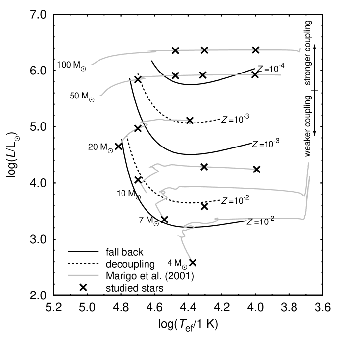
Figure 6: HR diagram for different types of stellar wind. Crosses denote studied stars, gray lines marked by corresponding mass are evolutionary tracks calculated by Marigo et al. (2001), solid lines denote approximate location of borders below which the fall back of hydrogen and helium occurs, and dashed lines denote approximate location of a border below which decoupling occurs (for a given mass fraction of heavier elements).

A HR diagram showing the different types of stellar wind is given in Fig. 6. For evolved stars of the highest luminosities, the multicomponent effects are important only for very low metallicities of the order of $Z\approx 10^{-4}$. On the other hand, for less-massive stars decoupling can occur even for a mass fraction of heavier elements comparable to the solar one ($Z\approx 10^{-2}$). The shape of border lines in Fig. 6 is given mainly by the mass-loss rate, and partly also by the terminal velocity, wind temperature, and charge. On average, decoupling occurs for mass fraction of CNO elements lower than roughly

$$\log Z_{\text{dec}}\approx\left[0.48-0.60\log\left(\frac{L}{1\,\text{L}_{\odot}}\right)\right]\\ \times\left[1+1.49\left(\frac{T_{\text{eff}}}{10^{5}\,\text{K}}\right)-3.1\left(\frac{T_{\text{eff}}}{10^{5}\,\text{K}}\right)^{2}\right].$$ (20a)

For even lower metallicities, lower than

$$\log Z_{\text{back}}\approx\left[0.40-0.65\log\left(\frac{L}{1\,\text{L}_{\odot}}\right)\right]\\ \times\left[1+1.49\left(\frac{T_{\text{eff}}}{10^{5}\,\text{K}}\right)-3.1\left(\frac{T_{\text{eff}}}{10^{5}\,\text{K}}\right)^{2}\right],$$ (20b)

the passive component decouples from hydrogen and helium for velocities smaller than the escape speed and may fall back onto the stellar surface.

5 Discussion

5.1 Wind limits

There exists a limiting mass-loss rate of heavier elements $\dot{M}_{\text{i}}^{\text{max}}$ below which hydrogen and helium remain in the stellar atmosphere and a purely metallic wind exists with a mass-loss rate $\dot{M}_{\text{i}}<\dot{M}_{\text{i}}^{\text{max}}$. As shown by Unglaub (2008), to achieve a hydrostatic hydrogen solution in the atmosphere, the magnitude of the gravitational acceleration should be larger than that of the hydrogen acceleration due to friction with heavier elements, i.e.,

$$\frac{GM}{r^{2}}>\frac{{n}_{\text{H}}{n}_{\text{i}}}{\rho_{\text{H}}}\frac{4\pi{q}_{\text{H}}^{2}{q}_{\text{i}}^{2}}{kT_{\text{Hi}}}\ln\Lambda\,G(x_{\text{Hi}}).$$ (21)

Using the same approximations as in Eq. (19) and the continuity equation, we obtain the condition

$$\dot{M}_{\text{i}}<\dot{M}_{\text{i}}^{\text{max}}=3\sqrt{\frac{\pi m_{\text{H}}}{2}}\frac{Gk^{3/2}}{q_{\text{H}}^{2}\ln\Lambda}\frac{m_{\text{i}}MT^{3/2}}{q_{\text{i}}^{2}}\\ \approx 3\times 10^{-17}\,\text{M}_{\odot}\,\text{year}^{-1}\!\left(\!\frac{m_{\text{i}}}{m_{\text{H}}}\!\right)\!\!\left(\!\frac{M}{1\,\text{M}_{\odot}}\!\right)\!\!\left(\!\frac{T}{10^{4}\,\text{K}}\!\right)^{3/2}\!\!\left(\!\frac{q_{\text{i}}}{q_{\text{H}}}\!\right)^{-2}.$$ (22)

Since in most considered cases in this study the derived mass-loss rate of heavier elements is higher than $\dot{M}_{\text{i}}^{\text{max}}$, hydrogen (and also helium, see Sect. 5.4) are driven out of the stellar atmosphere for the metallicities studied here. Subsequently, they may leave the star if there is no decoupling or if decoupling occurs for velocities larger than the escape value.

For metallicities lower than those studied here, the radiative force is, however, insufficiently strong to drive the wind containing the hydrogen and helium ions. At these very low metallicities, purely metallic winds may occur, if the radiative acceleration is large enough. The mass-loss rate of such a wind is lower than that given by Eq. (22). Since this condition does not depend on density, we note that the value of the limiting metallic mass-loss rate $\dot{M}_{\text{i}}^{\text{max}}$ is nearly constant throughout the stellar atmosphere (with some variations caused only by the temperature and charge variations).

5.2 Mass-loss rate and evolutionary calculations

From this and previous studies (Krtička & Kubát 2006, Paper I), we obtain the following picture of the stellar winds of hot first stars with an initially pure hydrogen-helium composition.

Pure hydrogen-helium stars do not have any line-driven wind. Stars very close to the Eddington limit with $\Gamma\gtrsim 0.859$ can have very weak ($\dot{M}\lesssim 10^{-14}\,\text{M}_{\odot}\,\text{year}^{-1}$) pure hydrogen winds due to light scattering on free electrons (Krtička & Kubát 2006). As a result, the influence of winds on the evolution of these stars is negligible. In rotating stars, mass loss by means of a decretion disk (Lee et al. 1991, Ekström et al. 2008) may be of some importance. Furthermore, massive stars may lose mass by means of either a $\eta$ Car type of explosions (Vink & de Koter 2005, Smith & Owocki 2006) or a super-Eddington outflow (Owocki et al. 2004). This outflow may more easily exist in evolved stars as the nuclearly processed core has a lower number of free electrons per nucleon than the hydrogen-rich envelope.

As soon as heavier elements are synthesised in the stellar core and transported to the stellar surface, a pure metallic wind may be produced (Babel 1995) if the radiative force on metals is large enough. These very weak stellar winds have mass-loss rates lower than those given by Eq. (22) (see also Unglaub 2008). Although this type of outflow probably does not influence stellar evolution, it may influence the stratification of the stellar atmosphere (e.g., Landstreet et al. 1998).

For metallicities higher than those given by Eq. (18) of Paper I, wind that also contains hydrogen and helium may exist. For metallicities lower than those given by Eq. (20b), the wind is very weak, wind decoupling occurs at velocities lower than the escape value, and hydrogen and helium may fall back on the stellar surface. The final fate of such a wind is however unclear because realistic simulations describing their behavior are not yet available.

For metallicities higher than those given by Eq. (20b), either winds are denser and decoupling occurs at velocities larger than the escape value or there is no decoupling at all. The wind mass-loss rate is given by the formulae of, e.g., Vink et al. (2001), Kudritzki (2002), or Paper I.

5.3 High velocity particles in primordial minihaloes

After decoupling, the CNO particles may be accelerated to velocities of the order of $v\approx 10^{4}\,\text{km}\,\text{s}^{-1}$, i.e., about $0.1c$. The energies of these particles are of the order of $1\,\text{MeV}$, and the consequent decoupling of the wind components produces the first low-energy cosmic-ray particles. The slowing-down time of these particles in the primordial minihaloes can be considerably large. If the interstellar material were already ionised, the slowing-down time would be estimated to be (Diver 2001)

$$\tau_{\text{s}}\approx\frac{m_{\text{i}}m_{\text{H}}}{4\pi q_{\text{i}}^{2}q_{\text{H}}^{2}n_{\text{H}}\ln\Lambda}v^{3}.$$ (23)

Assuming that the typical hydrogen densities inside minihaloes are of the order of $10^{2}\,\text{cm}^{-3}$ (e.g., Machacek et al. 2001), the slowing-down time is of the order of $10^{5}\,\text{years}$. Consequently, rapidly moving CNO particles may easily penetrate the halo and influence its chemical composition.

The aforementioned analysis is relevant if the influence of fast metallic wind on the interstellar medium can be neglected. In the opposite case, if acceleration of interstellar medium is non-negligible, the medium is swept up by a metallic wind, and its density increases. As a result, the slowing down time (23) shortens, the coupling between metals and interstellar medium strengthens, and the process repeats itself until a structure typical of wind-driven bubbles develops (e.g., Freyer et al. 2003). To assess the likelihood of this scenario, we calculate the ionized interstellar-hydrogen acceleration caused by its friction with the metallic wind to be (Burgers 1969)

$$g_{\text{fric}}=\frac{4\pi q_{\text{i}}^{2}q_{\text{H}}^{2}n_{\text{i}}}{m_{\text{H}}kT_{\text{Hi}}}\ln\Lambda G(x_{\text{Hi}})\approx\frac{q_{\text{i}}^{2}q_{\text{H}}^{2}\dot{M}_{\text{i}}\ln\Lambda}{m_{\text{i}}m_{\text{H}}^{2}r^{2}v^{3}},$$ (24)

where we used the approximate form of $G(x_{\text{Hi}})\approx 1/(2x_{\text{Hi}}^{2})$ valid for $x_{\text{Hi}}\gg 1$ and the continuity equation of metals. Writing the metallic mass-loss rate as $\dot{M}_{\text{i}}=\zeta\dot{M}_{\text{i}}^{\text{max}}$ (see Eq. (22)), the frictional acceleration is

$$g_{\text{fric}}=\frac{3\sqrt{\pi}}{4}\zeta\frac{a^{3}}{v^{3}}g(r),$$ (25)

where we have neglected the difference in charges between atmosphere and interstellar medium, and $g(r)$ is the magnitude of the gravity acceleration at a given point. Although $\zeta$ may be of the order of $10^{2}$, the ratio of the thermal speed in the atmosphere to the metallic wind velocity is $a/v\approx 10^{-3}$. Hence, the frictional acceleration of the interstellar medium is seven orders of magnitude lower than the gravitational acceleration and does not significantly influence the dynamics of the interstellar medium.

For homogeneous winds (i.e., those also including hydrogen), both the mass-loss rate and the ratio $a/v$ are larger. In this case, the frictional force influences the dynamics of the interstellar medium, the slowing-down time of Eq. (23) is short, and the problem becomes a hydrodynamical one.

5.4 He-free winds of cool stars?

Being heavier and less fragile than neutral hydrogen, neutral helium may remain in the stellar atmosphere, while hydrogen flows with heavier elements in the stellar wind. Taking into account that collisions with hydrogen are more important for helium acceleration than collisions with heavier elements, helium remains in the stellar atmosphere if (Krtička & Kubát 2004, c.f. Eq. (21))

$$\frac{GM}{r^{2}}>\frac{{n}_{\alpha}{n}_{\text{H}}}{\rho_{\alpha}}\frac{4\pi{q}_{\alpha}^{2}{q}_{\text{H}}^{2}}{kT_{\text{H}\alpha}}\ln\Lambda G(x_{\text{H}\alpha}),$$ (26)

where the subscript $\alpha$ denotes quantities corresponding to helium. Using the approximate formula for $G(x_{\text{H}\alpha})$ and the hydrogen continuity equation, we obtain a condition for the hydrogen mass-loss rate

$$\dot{M}_{\text{H}}<3\sqrt{\frac{\pi m_{\text{H}}}{2}}\frac{m_{\alpha}Gk^{3/2}}{q_{\text{H}}^{2}\ln\Lambda}\frac{MT^{3/2}}{q_{\alpha}^{2}}\\ \approx 10^{-16}\,\text{M}_{\odot}\,\text{year}^{-1}\left(\frac{M}{1\,\text{M}_{\odot}}\right)\left(\frac{T}{10^{4}\,\text{K}}\right)^{3/2}\left(\frac{q_{\alpha}}{q_{\text{H}}}\right)^{-2}.$$ (27)

From this, it seems that if the helium charge $q_{\alpha}$ is very low, i.e., if most of the helium atoms are neutral, then helium may remain in the stellar atmosphere, while hydrogen and heavier elements produce a wind. The other possibility of helium-free wind, i.e., a very low hydrogen mass-loss rate $\dot{M}_{\text{H}}\lesssim 10^{-16}\,\text{M}_{\odot}\,\text{year}^{-1}$, is not possible here because all studied stars have mass-loss rates higher than this value.

However, if helium atoms are neutral, collisions between neutral helium atoms and ionised hydrogen can accelerate helium into the stellar wind. Neutral helium remains in the stellar atmosphere if the magnitude of the frictional acceleration is smaller than the magnitude of the gravity force, i.e.,

$$\mu_{\text{H}\alpha}n_{\text{H}}n_{\alpha}\langle\sigma v\rangle_{\text{H}\alpha}v_{\text{H}}<\frac{\rho_{\alpha}GM}{r^{2}},$$ (28)

where $\mu_{\text{H}\alpha}=m_{\text{H}}m_{\alpha}/(m_{\text{H}}+m_{\alpha})$ is the reduced mass, and $\langle\sigma v\rangle_{\text{H}\alpha}$ is the momentum transfer rate coefficient for collisions between neutral helium and protons (Pinto & Galli 2008, Krstić & Shultz 1999). Adopting $\langle\sigma v\rangle_{\text{H}\alpha}\approx 10^{-9}\,\text{cm}^{3}\,\text{s}^{-1}$ and using the continuity equation, the condition given by Eq. (28) can be rewritten as

$$\dot{M}_{\text{H}}<4\pi GM\frac{m_{\text{H}}+m_{\alpha}}{\langle\sigma v\rangle_{\text{H}\alpha}}\\ \approx 2\times 10^{-13}\,\text{M}_{\odot}\,\text{year}^{-1}\left(\frac{M}{1\,\text{M}_{\odot}}\right).$$ (29)

For cooler massive stars, collisions between neutral helium and protons alone are able to accelerate helium if the wind is strong enough.

In models of cooler stars that we have studied, there is indeed a large fraction of neutral helium, but the charge of ionized helium is always high enough to accelerate helium into the wind (see Eq. (27)). For stars cooler than those studied here (with $T_{\text{eff}}<10^{4}\,\text{K}$), collisions of neutral helium with protons dominate the acceleration of helium in the stellar wind.

5.5 Charging of first stars and first magnetic fields

The problem of the escape of electrons from the stellar atmosphere was considered by Milne (1923, see also ). He demonstrated that electrons, due to the radiative forces acting on them, can escape from the star. However, he concluded that the resulting positive charge of the star would soon prevent any additional loss. The problem of charging the first stars by means of their winds remains an interesting one because of its possible implications for generation of the first magnetic fields.

Our models of the multicomponent stellar wind do not allow us to check the possibility of a star increasing its charge, since the zero current condition was used to determine the electron velocity at the wind base. The possible inclusion of an electron regularity condition corrupts (although only very slightly) the zero current condition at the upper boundary and can lead to the charging of the star.

However, the physical significance of both the electron critical point and the regularity conditions is questionable. From the hydrodynamic point of view, these conditions can only be used if they correspond to the point where the propagation speed of some type of disturbance is met. In general, the characteristic equations for the multicomponent flow may not necessarily describe the dissemination of the waves (e.g., Krtička & Kubát 2002). Thus, hydrodynamical simulations (or at least a linear analysis of hydrodynamical equations) should be used to prove the significance of the electron critical point condition. Only an analysis of this type will be able to answer the question of whether stellar charging via stellar winds is conceivable. However, if the possibility of stellar charging via stellar winds were proven, it could lead to the creation of first magnetic fields in the Universe.

5.6 The effect of wind inhomogeneities

We have modelled hot star winds by neglecting small-scale inhomogeneities. These inhomogeneities are expected on both theoretical (Owocki et al. 1988, Feldmeier et al. 1997) and observational grounds (Bouret et al. 2003, Martins et al. 2005, Puls et al. 2006). However, we expect that even in structured winds the inefficient transfer of momentum between the wind components may strongly affect the wind structure. We provide at least an estimate of the wind parameters for which these problems may occur and we outline the inclusion of these effects in the evolutionary calculations.

6 Conclusions

We have studied the effect of the Gayley-Owocki (Doppler) heating and multicomponent flow structure in CNO driven winds of hot stars. The parameters of these stars were selected to represent massive initially pure hydrogen-helium (Pop III) stars.

For the first time, we have included the GO heating term directly using atomic linelist and NLTE calculations. We have shown that GO heating is important especially for winds of CNO enriched first stars with high metallicities ($Z\approx 0.01$). In these winds, the GO heating can compete with radiative cooling because both the number of strong lines and the wind terminal velocity are large. On the other hand, for stars with low metallicities ($Z\lesssim 0.001$) there are an insufficient number of strong lines and the adiabatic cooling dominates.

The effects of multicomponent flows are important especially at low metallicities ($Z\lesssim 0.001$) in the case of evolved stars, and for relatively high metallicities ($Z\approx 0.01$) for main-sequence stars. The frictional heating itself does not influence the wind mass-loss rate. On the other hand, decoupling probably leads to a zero mass-loss rate of hydrogen and helium if it occurs at velocities lower than the escape one. We have developed an approximate formula that estimates the minimum metallicity above which hydrogen and helium leave the star.

The decoupling of radiatively accelerated metals from hydrogen and helium leads to generation of particles with typical energies of the order of 1 MeV, i.e., the first stars may be the first sources of low-energy cosmic rays. We have shown that these particles easily penetrate the interstellar medium of a given minihalo. We have discussed the possibility of charging of first stars via their multicomponent winds.

Wind models presented here can also be used to describe the winds of possible subsequent generations of CNO rich stars and low-luminosity stars of solar chemical composition.