Nuclear forward scattering in particulate matter: dependence of lineshape on particle size distribution

Abstract

In synchrotron Mössbauer spectroscopy, the nuclear exciton polariton manifests itself in the lineshape of the spectra of nuclear forward scattering (NFS) Fourier-transformed from time domain to frequency domain. This lineshape is generally described by the convolution of two intensity factors. One of them is Lorentzian related to free decay. We derived the expressions for the second factor related to Frenkel exciton polariton effects at propagation of synchrotron radiation in Mössbauer media. Parameters of this Frenkelian shape depend on the spatial configuration of Mössbauer media. In a layer of uniform thickness, this factor is found to be a simple hypergeometric function. Next, we consider the particles spread over a 2D surface or diluted in non-Mössbauer media to exclude an overlap of ray shadows by different particles. Deconvolving the purely polaritonic component of linewidths is suggested as a simple procedure sharpening the experimental NFS spectra in frequency domain. The lineshapes in these sharpened spectra are theoretically expressed via the parameters of the particle size distributions (PSD). Then, these parameters are determined through least-squares fitting of the line shapes.

1
1.Introduction1.1. Synchrotron Mössbauer spectroscopy and lengths distribution

Electronic and structural properties of materials were widely studied by Mössbauer spectroscopy in recent 50 years. Nuclear probe placed into deep structure scale interacts with its environment enabling to quantify the hyperfine interactions with unprecedented energy resolution. Cutting edge time domain Mössbauer spectroscopy using a synchrotron source has a potential of even twice better resolution. This is because the synchrotron Mössbauer spectra show no linewidth contribution from radioactive source, and only the linewidth contribution of absorber sample remains. For this reason the spectra obtained in time domain and Fourier-transformed to frequency domain might have narrower linewidths compared to conventional energy spectra measured in velocity scale.

Another attractive feature of the time-domain Mössbauer spectroscopy, to be explored in this work, consists in the possibility of studying the particulate matter. The point is that the length of the pathway through the resonant media is also reflected in nuclear resonant scattering[1]. The NFS theory [1] predicts in time domain the occurrence of the dynamic beats with periods depending on the lengths of radiation pathway. The pathway-dependent beats interfere with quantum beats originating from the quantum hyperfine splitting of nuclear levels.

In this work, the possibility of obtaining the information on the particle size distribution (PSD) from NFS is explored. Distribution of electronic and nuclear densities can be characterized by small-angle scattering (SAS) of x-rays and neutrons, respectively. In contrast, the unique feature of the method proposed here consists in determining the chemically-specific densities of resonant nuclei. Ferro- or aniferromagnetic ordering sensed by Fe spins in magnetic materials is probed using the ⁵⁷Fe nuclei. Therefore, our approach is relevant to various natural or synthetic magnetic compounds, doped by iron isotope, or containing iron intrinsically. Particularly, in application to multiphase systems, where at least one of the phases contains iron, there appears a unique chance of getting deeper insight into the interfacial structure. Thus, the proposed method has the potential to make a substantial contribution to experimental research both in multi- and single-phase systems.

Consider the nuclide-embedding particles placed into the synchrotron beam in a way that excludes the ray shadowing of one particle by another. The averaged over distribution chord lengths $d(\zeta)$ determines the total intensity of resonant scattering in forward direction.

In SAS, the distributions of nuclear or electronic densities $d_{\text{n}}(\zeta)$, $d_{\text{e}}(\zeta)$ are proportional to the second derivative of the SAS correlation function $\gamma_{0}(r)$:

$$d_{\text{n,e}}(r)=\frac{1}{\overline{\zeta}}\frac{d^{2}\gamma_{0}(r)}{dr^{2}}$$ (1)

Here $\gamma_{0}(r)=\gamma(r)/\gamma(0)$ and $\gamma(r)$ is self-convolution of density distribution[2]. The proportionality factor $1/\overline{\zeta}$ is the inverse mean length among all the particle chords distributed between $0$ and the maximum particle dimension $D$:

$$\overline{\zeta}=\int_{0}^{D}\zeta d(\zeta)d\zeta$$ (2)

In our case, $\overline{\zeta}$ is the average thickness of the resonant media. The condition of ”no shadowing” makes the chord lengths distribution (CLD) of randomly oriented particles equivalent to the resonant-media thickness distribution (RTD). In samples without mixing the resonant and non-resonant media, the RTD is quite analogous to the thickness distribution introduced previously in x-ray spectroscopy for thickness-related corrections of x-ray absorption spectra (XAS)[3]. While the thickness distribution determines the XAS and NFS spectra, the CLD is known to underlie, except SAS, a variety of properties of porous matter: conductivity, transport and relaxation. Investigating the CLD is subject matter of a special geometric sphere of knowledge[4].

2 1.2. Frequency-domain NFS spectra: the lineshapes

In this work, we limit ourselves to the case of full coincidence between thickness and chord lengths distributions (RTD$\equiv$CLD). For example, this is the case of single layer of particles spread over a surface or Mössbauer particles well diluted in non-Mössbauer media to avoid shadowing of one particle by another. This case includes not only the spherical particles of various particle size distributions (PSD’s), but also a network of wires or filaments viewed as discs in the plane perpendicular to the beam propagation direction. The relationships between the PSD, CLD and curves of SAS are known as solutions of the corresponding inverse scattering problems[2]. In a similar way, we will establish the relationship between PSD, CLD and the parameters of lineshape in the Fourier-transformed NFS spectra, such as shown in Fig. 1 (b).

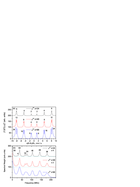
Figure 1: (a) Energy dependence of the NFS intensity in case of scatterer with the sextet of resonance lines of the transition probabilities 3:2:1:1:2:3. Due to the multiple scattering each resonance shows the double-hump structure at large $z$. The spectrum was obtained by squaring the absolute value of the Fourier-transformed sum of Eq. (3). It was verified that exactly same spectra can be obtained using the formula (Eq. 7) for squared transmission amplitude: $\left|1-R^{s}(E)\right|^{2}=\left|1-\exp\left(-i\sum_{l}\frac{\xi_{l}\Gamma_{0}}{E-E_{l}+i\Gamma_{0}/2}\right)\right|^{2}.$ Here $\Gamma_{0}$ is the linewidth ( $0.097$ mm/s in ⁵⁷Fe). The individual Mössbauer thicknesses $\mu_{l}z$ for each nuclear transition are indicated. Total dimensionless thicknesses of 24, 48 and 96 are given by the sum over all transitions $\mu^{\text{tot}}z=\Sigma\mu_{l}z$. (b): Frequency dependence of the NFS Fourier spectra, obtained using the same parameters of thickness and hyperfine interactions (magnetic hyperfine field $H_{\text{hf}}$=500 kOe, quadrupole splitting $\varepsilon=0$).

Our approach to the NFS data treatment in frequency domain is very different from the conventional one, that has been known since the first observations of quantum beatings[5, 6, 7]. In the frequency domain, we show that a single quantum beat can be disentangled from the complex sum of beatings at the condition of large enough hyperfine fields ($H_{\text{hf}}\gtrsim 200$ kOe). Fitting the lineshape for any individual line of the Fourier spectra permits to determine the RTD parameters even for complex distributions of thickness of the resonant media.

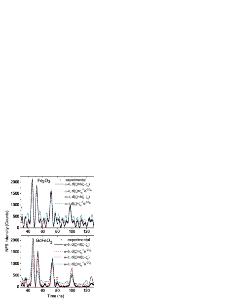
Figure 2: NFS spectra of Fe₂O₃ and GdFeO₃ fitted using the theoretical intensities derived from the Eqs. (5) and (6). The goodness of fit is always best for $\alpha=0$. Except the experimental spectra and fitted theoretical spectra for $\alpha=0$, the simulated spectra for $\alpha=1$ nm/$\mu$m (Fe₂O₃) and $\alpha=2$ nm/$\mu$m (GdFeO₃) are also shown. The unenriched oxides Fe₂O₃ and GdFeO₃ contain the density of the ⁵⁷Fe nuclei by 100 and 230 times smaller than that in bcc metal of $\alpha-^{57}$Fe.

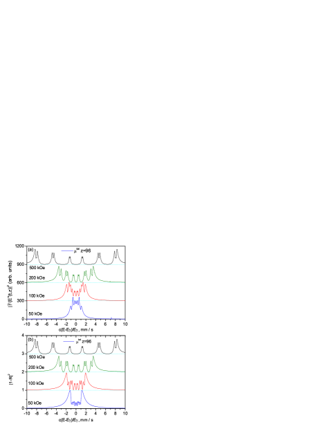
Figure 3: Energy spectra of the scattered radiation corresponding to approximate (a) and exact (b) solutions of the wave equation for radiation pulse propagating through resonant media. The squared amplitudes of radiation field vs. energy are calculated using the Eqs. (5) and (7) in (a) and (b), respectively. Note the coincidence of spectra in (a) and (b) for $H_{\text{hf}}$ $\gtrsim$ 200 kOe.

3 3.Prerequisites3.1. The approximation of singular magnetic hyperfine fields

Already the first studies of NFS[10] showed that a phenomenon of coupling between quantum beats and dynamical beats often takes place at large lengths of radiation pathways through the resonant media. This hybridization results from broad magnetic-hyperfine-field distributions that have a strong effect on the time evolution of the intensity of the forward scattered radiation. This is the case of magnetic alloys having essentially disordered atomic structure, such as Invar, or fully amorphous alloys and compounds. Distribution of quadrupole parameters in nanoparticles or in deformed crystals is another example of inhomogeneous broadening that gives rise to the coupling between quantum and dynamical beats. In what follows, we disregard these cases to focus on the case of singular value of hyperfine magnetic fields for all the ⁵⁷Fe nuclei involved.

4 2.2. The approximation of large magnetic hyperfine fields

Even for a singular values of hyperfine fields the radiation scattered forward in samples of large thickness exhibits a broad energy distribution around each hyperfine transition, showing the so-called double-hump picture of a hyperfine transition (Fig.1, a). This picture arises from solving the wave equation for propagation of a radiation pulse through a resonant medium[10]. Closed analytic solutions of corresponding wave equations exist only for a single-line resonance. However, if we remain in the limit of large energy separation between the hyperfine transitions, there exists a good approximation to the analytic solution even in the case of multiple resonances. This approximation is applicable when the energy separation between different transitions is large enough compared to natural linewidth [8, 9, 10].

Then the approximate solution for the field amplitude of the radiation scattered in forward direction can be expressed as follows[10]:

$$E^{s}(t,z)\propto\sum_{l}\mu_{l}z\exp(-\frac{i}{\hslash}\Delta E_{l}t-\frac{\tau}{2})\frac{J_{1}(\sqrt{\mu_{l}z\tau})}{\sqrt{\mu_{l}z\tau}}$$ (3)

Here the index $l$ numerates the nuclear transitions with the energy difference of $\Delta E_{l}$ between ground and excited states. The factor $e^{-\tau/2}$ describes the free-nucleus decay. The dimensionless time $\tau=t/t_{0}$ is expressed in units of free decay time $t_{0}$ (e.g., $t_{0}$=141.1 ns for ⁵⁷Fe). The nuclear absorption coefficient $\mu_{l}=$ $\sigma_{0}\rho f_{\text{LM}}\eta w_{l}$ is expressed individually for each transition using the weight factor $w_{l}$ of the $l$-th transition. The factor $w_{l}$ takes into account the probability partition between nuclear sublevels split by hyperfine interactions, so that $\Sigma_{l}w_{l}=1$. Other factors are the resonance cross section $\sigma_{0}$, the density of the resonant nuclei $\rho$, the Lamb-Mössbauer factor $f_{\text{LM}}$, and the resonant nuclide isotope abundance $\eta$.

The time and space variables are entangled in the Eq.(3) via the complex argument of the Bessel function of first kind and order one:

$$J_{1}(\sqrt{\mu_{l}z\tau})=\sum_{k=0}^{\infty}\frac{(-1)^{k}}{k!(k+1)!}\left(\frac{\sqrt{\mu_{l}z\tau}}{2}\right)^{2k+1}$$ (4)

Using the variable $\xi_{l}=\mu_{l}z/4$ the power series of the Bessel argument $\sqrt{\mu_{l}z\tau}/2$ can be replaced by the power series of $\sqrt{\xi_{l}\tau}$. The dimensionless parameter individual for each $l-$th transition $\xi_{l}$ is called the transition effective resonant thickness, resulting in radiation field:

$$E^{s}(t,z)\propto\sum_{l}\xi_{l}\exp(-\frac{i}{\hslash}\Delta E_{l}t-\frac{\tau}{2})\frac{J_{1}(2\sqrt{\xi_{l}\tau})}{\sqrt{\xi_{l}\tau}}$$ (5)

In terms of Eq.(5), the spectra shown in Fig. 1 (a) represent the squared absolute values of the corresponding Fourier transforms $\left|\mathcal{F}(E^{s}(t,z))\right|^{2}$. The values of effective resonant thickness $\mu_{l}z$ are $l-$specific and proportional to the relative intensity of the Mössbauer line for the $l$-th transition. Three values of total Mössbauer thickness ($\mu^{\text{tot}}z=\Sigma_{l}\mu_{l}z=24,48$ and 96) are used to draw the Fig.1. The magnetic hyperfine field of 500 kOe and zero quadrupole splitting are assumed. Very close hyperfine parameters were observed previously in GdFeO₃[11]. Spectral weight of the quantum beat frequency spectra shown in Fig.1 (b) represents the $\cos$-Fourier transform of the squared sum in right-hand of Eq.(3). Information contained in such Fourier images is the same as in experimental data. In what follows, we elaborate the concept of lineshape in these Fourier spectra.

5 2.3. Are the shifts of quantum beat occuring in forward scattering?

The (Eq.5) was introduced in 1998 by Shvyd’ko et al (see, Eq. (16) in the work [10]). In the Eq.(5), the radiation field $E^{s}(t,z)$ exhibits at the time $t=0$ similar phase for each $l^{\text{th}}$ transition. The same assumption was used in Refs. [6],[11, 12, 13]. However, some of the previous works [7, 8] supposed the existence of a finite difference between the initial phases (at $t=0$) for different transitions (see the Eq.(29) in Ref.[8]):

$$E_{\alpha}^{s}(t,z)\propto\sum_{l}\xi_{l}\exp\left(-\frac{i}{\hslash}\Delta E_{l}t-\frac{\tau}{2}+\alpha\sum_{m}\frac{\Gamma\xi_{m}}{\Delta E_{lm}}\right)\psi_{l}$$ (6)

Here $\psi_{l}$ is the same factor as in Eq.(5), $\psi_{l}$ $=J_{1}(2\sqrt{\xi_{l}\tau})/\sqrt{\xi_{l}\tau}$ and $\Delta E_{lm}$ is the energy difference between $l^{\text{th}}$ and $m^{\text{th}}$ transitions. In the experimental data for magnetized ⁵⁷Fe foils, the finite quantum beat shifts were claimed in two early works[7, 8], but not reported in precedent[6] and succeeding[10, 11, 13, 12] studies. Quite large values of the parameter $\alpha$ were reported for the NFS with a single QB component, $\alpha=0.133$ nm/$\mu$m [7] and $\alpha=0.14$ nm/$\mu$m[8] If such QB shifts were present for some of the QB components from sextet, the shape of the curve of sum-total NFS would distinctly depend on the thickness even in the absence of any distribution of thickness. In case of thickness distribution, the shift is expected to smear the quantum beats. On the other hand, no smearing is expected in case of validity of the zero-shift formula (Eq.5), which accounts for the thickness distribution only through the envelopes $\psi_{l}$.

No QB shifts were assumed previously at fitting the NFS data for powdered antiferromagnetic oxides[11]. Let us compare which of the Eqs. (5 and 6) fits better the experimental time spectra. In Fig 2, the NFS spectra of Fe₂O₃ and GdFeO₃ are fitted using both Eqs. (5 and 6). The goodness of fit is always best for $\alpha=0$. Except the experimental spectra and theoretical spectra for $\alpha=0$, the spectra for $\alpha=1$ nm/$\mu$m (Fe₂O₃) and $\alpha=2$ nm/$\mu$m (GdFeO₃) are also shown. Both these oxides were prepared with natural abundance of ⁵⁷Fe. The density of ⁵⁷Fe nuclei in such unenriched Fe₂O₃ and GdFeO₃ oxides is lower than in ⁵⁷Fe foil by the factors of 100 and 230, respectively. For each pair of transitions, $l$ and $m$, the terms $\alpha\Sigma_{m}(\Gamma\xi_{m}/\Delta E_{lm})$ are relatively small. In case of magnetic sextet of transitions with small quadrupole shift, there are three groups of sums $\Sigma_{m}(\Gamma\xi_{m}/\Delta E_{lm})$ with relative values of $\simeq 0$, $\simeq 1$, and $\simeq 2$. Each of these terms $\alpha\Sigma_{m}(\Gamma\xi_{m}/\Delta E_{lm})$ is smaller than the QB shift for $\alpha=0.133$ nm/$\mu$m in ⁵⁷Fe foil at least by an order of magnitude. Despite very small values of $\alpha$ assumed, Fig. 2 shows strong divergence between experimental and simulated for $\alpha\neq 0$ spectra. Shape of the time dependence of the squared field amplitude $E_{\alpha}^{s}(t,z)$ calculated from Eq.(6) exhibits very strong changes even for small deviations of $\alpha$ from 0. Such a variation of shape is the best measure for the value of $\alpha$. No significant deviation of $\alpha$ from $0$ is observed in our data shown in Fig.2. This is contrasting to the interpretations derived from the data in magnetized ⁵⁷Fe foil with just two unsuppressed transitions[7]. The complex shape of the NFS time spectra for magnetic sextet is a more reliable observation than the shift of QB reported for the magnetized ⁵⁷Fe foil doublet. In fact, experimental NFS data suffer generally from the uncertainty of time origin. This can be caused, for example, by a finite spread of prompt pulse. This uncertainty may lead to a misleading shift of spectra as a whole, however, may not change the shape of the NFS pattern.

Thickness distribution modeled by the exponential function $d(\xi)=$ $\xi_{0}^{-1}\exp(-\xi\xi_{0}^{-1})$ is consistent with the NFS spectra of Fe₂O₃, but inconsistent with the NFS spectra of GdFeO₃ (Fig.2). Except difference in quadrupole splitting (cf. $\varepsilon=-0.1$ mm/s in Fe₂O₃ and $\varepsilon=+0.03$ mm/s in GdFeO₃ [11]) these samples differ by factor 4 in their Mössbauer thickness and by factor of 10 in their metric thickness. The thicker sample GdFeO₃ showed a disagreement with the assumption of exponential distribution. In such a thick sample, the particles were most probably stacked in several layers, shadowing each other. Resulting distribution is much closer to $\delta$-function than to exponential distribution. We obtained $\xi_{0}\simeq 22$ assuming the uniform thickness, $d(\xi)=\delta(\xi-\xi_{0})$. By contrast, in the thinner sample ( Fe₂O₃), the distribution of thicknesses about the mean value $\xi_{0}$was relatively broad. As the result, the fitting quality was equally good for $d(\xi)=\delta(\xi-\xi_{0})$ and $d(\xi)=$ $\xi_{0}^{-1}\exp(-\xi/\xi_{0})$ when the fitting is done in the time range between 30 and 130 ns (Fig .2). However, the exponential distribution suits better when the spectra were fitted in broader range. The parameters can be fitted either in time domain or in Fourier-transformed spectra. Below we present fitting the Fourier spectra as the most convenient and transparent method.

6 2.4. Exact energy spectra of the scattered radiation compared with the large-fields approximation

The condition of validity of the approximation (Eq.5) was given in 1998 by Shvyd’ko et al[10]. It was pointed out[10] that the Eq.(5) is valid even in the thick samples, if the nuclear transition energies $E_{l}$ are well separated from each other. This means that the condition of validity of Eq.(3) is the greatness of the magnetic hyperfine field compared to natural Lorentzian linewidth. Numerically, this statement is verified and confirmed in Fig.3. Our calculations aimed to answer the question: how large fields are sufficient to apply the approximation? In Fig.3, the squared value of $\left|1-R^{s}(E)\right|$ is plotted, where $R^{s}(E)$ being the system response function:

$$R^{s}(t,z)=\exp\left(-i\sum_{l}\frac{\xi_{l}\Gamma_{0}}{E-E_{l}+i\Gamma_{0}/2}\right)$$ (7)

The Eq.(7) is the exact result, therefore, the Fig.3 presents the comparison between the approximate result $\left|\mathcal{F}(E^{s}(t,z))\right|^{2}$ (a) and the exact one $\left|1-R^{s}(E)\right|^{2}$ (b). Large value of thickness $\mu^{\text{tot}}z=96$ was chosen to plot the Fig.3. Full coincidence of the exact result and analytic solutions is shown for $H_{\text{hf}}\gtrsim 200$ kOe.

7 3.Results3.1. Lineshapes of individual lines of the Fourier spectra for hyperfine sextet

In large hyperfine fields ($H_{\text{hf}}\gtrsim 200$ kOe), the difference between numeric and analytical solutions is negligible. Therefore, the squared sum over hyperfine transitions (Eq.3) can be converted into sum over the intertransitional pairs:

$$I(t,z)\propto z^{2}e^{-\tau}\sum_{n}A_{n}(z,\tau)\cos\varpi_{n}t$$ (8)

Fourier transformation of the Eq.(8) results in the quantum beat frequency spectra shown in Fig.1 (b). In case of pure magnetic hyperfine interactions, the quantum beats frequencies $\varpi_{n}$ and amplitudes $A_{n}(z,\tau)$ can be expressed via the parameters $\Omega=\frac{1}{4}g_{3/2}\mu_{N}H_{\text{hf}}/\hbar$ and $\psi_{j}=J_{1}(2\sqrt{j\xi_{\min}\tau})/\sqrt{j\xi_{\min}\tau}$ $(j=1,2,3)$ , respectively, as shown in the Table 1.

Table 1. The quantum beat frequencies $\varpi_{n}$ and amplitudes $A_{n}(z,\tau)$ for nuclear levels split by purely magnetic hyperfine interactions. The frequencies are expressed through $\Omega=\frac{1}{4}g_{3/2}\mu_{N}H_{\text{hf}}/\hbar$ and the amplitudes are expressed through $\psi_{j}=J_{1}(\sqrt{j\mu z\tau})/\sqrt{j\mu z\tau}$ $(j=1,2,3).\vskip 3.0pt plus 1.0pt minus 1.0pt$

$\varpi_{n}$	$A_{n}(z,\tau)$
0	$\psi_{1}^{2}+4\psi_{2}^{2}+9\psi_{3}^{2}$
3$\Omega$	$\psi_{1}^{2}$
4$\Omega$	$4\psi_{1}\psi_{2}+12\psi_{2}\psi_{3}$
7$\Omega$	$4\psi_{1}\psi_{2}$
8$\Omega$	$6\psi_{1}\psi_{3}$
11$\Omega$	$6\psi_{1}\psi_{3}+4\psi_{2}^{2}$
15$\Omega$	$12\psi_{2}\psi_{3}$
19$\Omega$	$9\psi_{3}^{2}$

There are eight spectral lines corresponding to eight nonidentical intertransitional energy differences for purely magnetic hyperfine interactions. According to the Table 1, each line in the frequency domain has its own lineshape. The line at highest frequency is the widest one. This line turns out to be most suitable for our analysis because the Fourier transformation of $\psi_{3}^{2}$ $=J_{1}^{2}(2\sqrt{\xi\tau})/\sqrt{\xi\tau}=J_{1}^{2}(2\sqrt{3\xi_{\min}\tau})/3\xi_{\min}\tau$ can be found analytically. Here we denoted by $\xi$ and $\mu z$ the transition-specific quantities $\xi=$ $3\xi_{\min}=\mu z/4=\mu^{\text{tot}}z/16.$By the minimum thickness, $\xi_{\min}=\mu^{\text{tot}}z/48$ we denoted the thickness of the weakest transition (1 in the notation 3:2:1:1:2:3).

In presence of quadrupole interactions some of these eight lines split into doublets and triplets to produce fourteen lines, however, the line of highest frequency always stands alone. This outstanding feature makes it easy to apply the suggested here analysis in frequency domain. It is from this line the parameters of thickness distribution are derivable most easily.

8 3.2. The shape and width of highest-frequency line

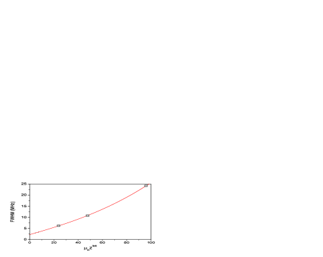
Figure 4: Thickness dependence of the full-width-at-half-maximum (FWHM) of the highest-frequency line shown in Fig.1(b). The lineshape is the convolution of the thickness-independent Lorentzian and thickness-dependent term $\left|1-_{2}\digamma_{3}[\{\frac{1}{3},\frac{3}{4}\},\{\frac{1}{2},1,\frac{3}{2}\},-\frac{\mu^{2}z^{2}}{4\omega^{2}}]\right|$ with ${}_{2}\digamma_{3}$ being the hypergeometric function. Pure Lorentzian contribution to the linewidth at $z=0$ is 2.26 MHz.

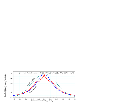
Figure 5: Comparison of the universal distribution functions normalized by both area and height: the ”Polaritonian”, obtained as Fourier transform of the QB envelope $\mathcal{F}(\psi_{3}^{2})=$ $1-_{3}F_{2}[\{\frac{1}{4},\frac{3}{4}\},\{\frac{1}{2},1,\frac{3}{2}\},-\frac{\mu^{2}z^{2}}{4(\omega-\omega_{0})^{2}}]$(continuous line), compared to Lorentzian $\frac{1}{\pi\Gamma}\frac{1}{1+(\omega-\omega_{0})^{2}/\Gamma^{2}}$(dashed line) and Gaussian $\frac{1}{\sqrt{2\pi\sigma^{2}}}\exp(-\frac{(\omega-\omega_{0})^{2}}{2\sigma^{2}})$ (dotted line).

In Eq. (8), except the functions $\psi_{j}$, the factor $e^{-\tau}$ contributes the lineshapes. Unlike the $\psi_{j}-$dependent factors individual for each line, the factor $e^{-\tau}$ is common for all NFS data, therefore, it can be easily removed by the sharpening procedure as shown below. Here we note that the $e^{-\tau}$-factor dominates the full-width-at-half maximum for small linewidths (FWHM $\lessapprox$ 5 MHz). Remaining factors shown in the Table 1 become predominant for larger linewidths. The Fourier images of these remaining factors are the $\Lambda-$shaped functions with some shoulders. In Fig.1(b), the shoulders start to be visible for the singlet line as the thickness increases. In the limit of zero thickness the Lorentzian contribution to the linewidth is 2.2575 MHz (Fig. 4). The plot of FWHM vs thickness is not linear because the thickness-dependent component differs in shape from the Lorentzian $L=\mathcal{F}(e^{-\tau})$.

Since the NFS spectra are defined for $t>0$  the Fourier-transform is defined as $\mathcal{F}(f)=\sqrt{2/\pi}\int_{0}^{\infty}f(t)\cos(\omega t)dt$. For the sake of normalization of the line intensities in Fourier spectra we introduce the new variable $\zeta$ that is another useful parameter related to Mössbauer thickness:

$$\zeta=\pi\xi=\frac{\pi}{4}\mu z=\frac{\zeta^{\text{tot}}}{4}=\frac{\pi}{16}\mu^{\text{tot}}z\text{ .}$$ (9)

The new parameter $\zeta$ presents the measure of FWHM in the NFS Fourier spectra vs. angular frequency $\omega$. In contrast, the parameter $\xi$ is the suitable measure of FWHM in the NFS Fourier spectra vs. linear frequency. Transforming the NFS time spectra, Eq. (8), to the frequency domain one obtains a set of lines, whose lineshapes are represented by the convolution of the Fourier images of the free decay component and the thickness-dependent component. First component is the free-decay Lorentzian $L=\mathcal{F}[\exp(-\tau)]$ independent of the polaritonic parameter $\zeta$. Second is the polaritonic component related to propagation of radiation pulse through the resonant media. Because of this convolution the full lineshape can be found only by numerical calculations. For a single-line spectrum this was already done[11]. The spectral lineshape was shown to evolve with increasing thickness from the Lorentzian profile to a different profile (so-called $\Lambda$-shaped [11]). However, no analytic expression was obtained yet for the thickness-dependent component of the lineshape. This solution will be found in the present work. The method of determination of the thickness distribution parameters simply follows from this analytic solution.

In very thin samples, the same analysis could be applicable to the line at $\varpi_{n}=3\Omega\$shaped as simply as the Fourier-image of $\psi_{1}^{2}$, however, this line is just a tiny satellite of the strongest line of the NFS Fourier spectra (see Fig.1,b). That is why the operational range of thicknesses for this line is narrower than that for the line at $\varpi_{n}=19\Omega$. In sharpened NFS Fourier spectra, we could manage to find the analytic solution for the spectral shape of these two lines, the narrowest one and the widest one, but not for the other lines.

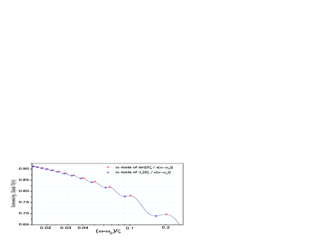
Figure 6: Center of the Polaritonian $1-h_{\frac{3}{2}}\left[-\frac{4\zeta^{2}}{\pi^{2}(\omega-\omega_{0})^{2}}\right]$ vs. $(\omega-\omega_{0})/\zeta$ (Eq. 11) in semilogarithmic scale. Maxima and minima in the oscillating behavior of the lineshape are indicated by up and down triangles, respectively.

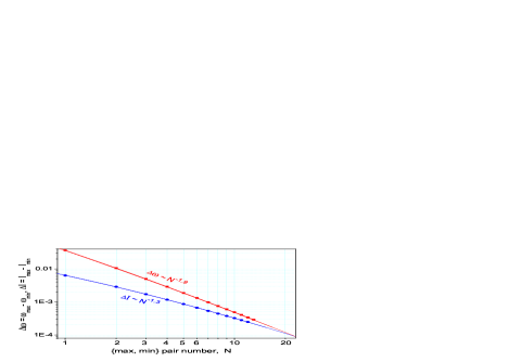
Figure 7: The widths $\Delta\omega$ and the heights $\Delta I$ of the satellite shoulders in the polaritonic lineshapes shown in log-log scale. The numeration counter of shoulders $N$ goes from outwards to the center of the spectral line. Shown on the plot are the power exponents calculated using $N=13$.

9 3.3 Shape of the polaritonic component for a uniform-thickness layer (foil)

Thus, since the sharpened lineshape is well-defined theoretically one can fit the sharpened data with a thickness-dependent analytic expression. Prior the Fourier transformation the experimental spectra are multiplied by the factor $\exp(\tau)$. Then the NFS sum for a uniform thickness $\zeta$ (Eq.8) will have the highest-frequency term as follows:

$$\widetilde{I}(t,\zeta)\exp(\tau)\propto\zeta^{2}\left(\frac{J_{1}\left(2\sqrt{\zeta\tau/\pi}\right)}{\sqrt{\zeta\tau/\pi}}\right)^{2}\cos 19\Omega t$$ (10)

This procedure allowed us to obtain in the frequency domain the lineshape deconvoluted from the natural decay Lorentzian. Therefore, in the frequency domain, instead of the intensities $I(\omega),$ calculated previously[11], we operate now with the sharpened intensities $I_{\text{sh}}$ $(\omega,\zeta)=$ $\allowbreak\mathcal{F}[\widetilde{I}(t,\zeta)\exp(\tau)]$. The Fourier transform of the remaining lineshape factor in the right hand side of the Eq.(10) has the functional form:

$$\allowbreak\mathcal{F}\left[\frac{\zeta}{\sqrt{2\pi}}\left(\frac{J_{1}\left(2\sqrt{\zeta\tau/\pi}\right)}{\sqrt{\zeta\tau/\pi}}\right)^{2}\right]=1-h_{\frac{3}{2}}\left(-\frac{4\zeta^{2}}{\pi^{2}\omega^{2}}\right)$$ (11)

Here $\omega$ is the dimensionless angular frequency corresponding to the dimensionless time $\tau$. By $h_{\frac{3}{2}}(x)$ we denoted the hypergeometric function ${}_{2}\digamma_{3}[\{\frac{1}{3},\frac{3}{4}\},\{\frac{1}{2},1,\frac{3}{2}\},x]$, using the last but one argument of the function as subscript. The value $\zeta=1$ in Eq.(11) correspond to the normalized, both in area and height, distribution density (Fig. 5). Similarly normalized Lorentzian and Gaussian distributions are $\left[1+\pi^{2}(\omega-\omega_{0})^{2}\right]^{-1}$ and $\exp\left[-\pi(\omega-\omega_{0})^{2}\right]$. The FWHM of the polaritonic function is slightly larger than FWHM of Lorentzian but smaller than that for Gaussian. To within this difference caused by the difference of the lineshape, the natural linewidth caused by the natural decay $\exp(-\tau)$ is equivalent to the thickness of $\zeta_{\text{eqv=}\tau}=\pi$ or $\xi_{\text{eqv=}\tau}=1$.  The origin of $\omega$ is located at the highest quantum beat frequency, hence, the positive and negative values of $\omega$ are measured relative to $\omega_{0}=19\Omega,$ that is not shown in Eq.(11). The same notation for $\omega$ will be used below ($\omega$ ”measuring” relative to $\omega_{0}$).

The polaritonic lineshape has a very sharp tip in the center and the wings decaying similarly to the Lorentzian. It has the main shoulders $I_{1}\approx 0.7I_{0}$ at $\omega_{1}\approx\omega_{0}\pm 0.2\zeta$. A sequence of less-marked shoulders exists in closer proximity to the resonance. These shoulders are formed by shallow minima and maxima at $\omega_{N}^{\min}$ and $\omega_{N}^{\max}$, respectively, as shown in semilogarithmic scale in Fig. 6. The maxima are located at $\omega_{N}^{\max}=\omega_{0}\pm 2\zeta/N\pi^{2}$, $N=1,2..\infty.$The minima are given by the roots of the equation:

$$J_{1}\left(\frac{2\zeta/\pi}{(\omega_{0}\pm\omega_{N}^{\min})}\right)=0$$ (12)

The width of the shoulders $\Delta\omega_{N}=$ $\omega_{N}^{\max}-\omega_{N}^{\min}$and the heights of the satellite peaks $\Delta I_{N}=$ $I_{N}^{\max}-I_{N}^{\min}$ decrease with N approximately as the power laws $N^{-1.9}$ and $N^{-1.3}$, respectively. Both curves $\Delta\omega_{N}$ vs. $N$ and $\Delta I_{N}$ vs. $N$ show a small curvature in the log-log scale (Fig. 7). They merge each other both in position and in slope as $N$ increases and the oscillations of $I(\omega)$ fade out with $\omega$ approaching $\omega_{0}$.

The NFS radiation field and the nuclear currents are the polaritonic subsystems feeding each other as the excitation pulse propagates through the resonant media[14, 15]. As the time elapses after the arrival of prompt pulse of synchrotron radiation the frequency of the energy exchange between these two subsystems at a fixed coordinate $z$ decreases. The nodes and antinodes change each other less and less frequently. The region of small frequencies in the NFS Fourier spectra is dominated by the harmonics from large $\tau$ of the NFS time spectra. Lorentzian shape in frequency domain correspond to $\exp(-\tau)$ in time domain and, vice versa, the Lorentzian’s decay asymptotic $\tau^{-2}$ would produce around $\omega_{0}$ the triangularly peaked shape $\exp(-\left|\omega-\omega_{0}\right|)$. In Fig. 5, we observe that the peak is ever sharper than triangular. Taking the function $\psi_{3}^{2}(\tau)$ at the points of antinode maxima we observe that $\psi_{3}^{2}(\tau_{\text{a}})$ decays with $\tau$ as $\tau^{-3/2}$, i.e., even slower than the Lorentzian’s asymptotic $\tau^{-2}$. Indeed, one can check that the Fourier transformation of the function $(1+|\tau|^{\frac{3}{2}})^{-1}$ gives a very sharp peak, similar to that of Fig. 5, but free of the oscillations investigated in Figs 6 and 7.

10 3.4 Deconvolving the polaritonic component using the technique of sharpening of the experimental Fourier spectra

Sharpening the NFS Fourier spectra is shown in Fig. 8 for the data collected from unenriched Fe₂O₃ with natural abundance of ⁵⁷Fe. The spectra were first fitted in the experimental time domain $0.18<\tau<3$ and then extrapolated to the short-delay region, $\tau<0.18$. Missing original data for the $\tau<0.18$ caused by the prompt flash overshooting detector were thus restored. The expression for fit function was given previously (see Eq.(28) in Ref. [11]). Instead of 8 lines for $\varepsilon=0$ there are actually 14 lines for the combined magnetic and quadrupole Hamiltonian. The fitted quantum beats parameters are $H_{\text{hf}}=517.5$ kOe and $\varepsilon=-0.1$ mm/s. Due to the smallness of $\varepsilon$ the lines are grouped into 2 symmetric triplets, 2 symmetric doublets and four singlets. The doublets and triplets are clearly distinguished in the sharpened spectra.

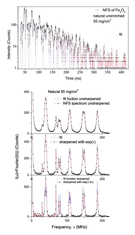
Figure 8: NFS spectra of the Fe₂O₃ powder and their unsharpened and sharpened Fourrier transforms. Top panel data are from [11]. The data are plotted vs. linear frequency, to be distinguished from $\omega$ in Figs. 1-3. The datapoints in lower panel are obtained via fast Fourier transforms of NFS time spectra according to formula $I_{j}=\frac{1}{n}\Sigma_{k}\widetilde{I}_{k}e^{-i(2\pi j/m)k}$ with the number of channels in NFS spectra $m$=4096. Solid (blue) line is the sum of Lorentzians of different widths $\zeta_{\text{eff}}^{2}$ fitted individually for each of 14 lines. Each Lorentzian is the Fourier image of the time-domain exponential function fitting the individual quantum beat envelope: $\mathcal{F}\left[\frac{\zeta_{\text{eff}}}{\sqrt{2\pi}}\exp(-\zeta_{\text{eff}}\tau/\pi)\right]=\frac{\zeta_{\text{eff}}^{2}}{\zeta_{\text{eff}}^{2}+\pi^{2}\omega^{2}}.$The constraints between the parameters of $\zeta_{\text{eff}}$ for different lines was used to reduce the number of parameters from 14 to one thickness parameter (see Eq.28 in Ref. [11]).

From the viewpoint of theory the $\exp(-\tau)$-sharpened spectrum in the middle panel of Fig. 8 must possess the purely polaritonic lineshape. The factor $\exp(\tau)$ permits us to isolate the polaritonic lineshape in its undistorted form predicted by the theory. In the middle panel of Fig. 8, the largest-frequency line at $\varpi_{n}=19\Omega$ possess the largest polaritonic linewidth $\zeta=3\zeta^{\min}=$ $4.86$.

The sharpening technique is also very useful for the illustration of the relationship between the width of different spectral lines. To the first approximation we can neglect the non-linearity in the plot of FWHM vs thickness in Fig. 4 and assume the additivity of the Lorentzian and polaritonic linewidths. Therefore, deliberately, the spectrum might be further sharpened using the exponent larger than $\exp(\tau)$ in Eq.(10). Such a heuristic sharpening is shown for the sharpening factor $\exp(3\tau/2)$ in the bottom panel of Fig. 8. The residual linewidth of the narrowest line at $\varpi_{n}=3\Omega$  became very small ($\zeta_{\text{res}}\simeq 0.05$). Such an oversharpening is equivalent to subtraction of $3\pi/2$ from the linewidth, while the theoretic $\exp(\tau)$-sharpening correspond to subtraction of $\pi.$ According to the Table 1, the polaritonic linewidths determined by the function $\psi_{3}^{2}$ is three times larger than the polaritonic linewidths determined by the function $\psi_{1}^{2}$. This relationship gives us the following equation for the polaritonic linewidths of the lines at $\varpi_{n}=3\Omega$ and $19\Omega$:

$$3\left(0.05+\frac{\pi}{2}\right)=4.86$$ (13)

This relationship is in full agreement with our observation in Fig. 8.

In the middle panel of Fig. 8, there appear only a few experimental points per FWHM of a spectral line. Two questions are remaining in this respect. First of all, it is natural to ask how the appearance of spectra can be improved. What kind of experimental limitations should be lifted over to raise the number of experimental points per FWHM? Second, we must indicate the way how to apply the analysis in practice for determination of the particle distribution characteristics.

11 3.5 Effects of temporal range cut-off and resolution in frequency

Generally, the interval $\Delta\omega$ between points of the discrete Fourier spectra is inverse total sample time:

$$\Delta\omega=\frac{2\pi}{m\Delta\tau}$$ (14)

In NFS, the value $\tau_{\max}=m\Delta\tau$ is limited by the interval between bunches of electrons of the storage ring. The data of Fig. 8 were collected in single-bunch regime[11], with the interval between bunches of 500 ns and $\tau_{\max}=3.54.$ This experimental restriction on $\tau_{\max}=m\Delta\tau$ determines the number of points per FWHM. The number of channels $m=4096$ defines the NFS sampling frequency. According to the ‘uncertainty principle’, Eq.(14), the increase in the value of $m$ will not influence the number of points per FWHM. However, in very thick samples, approximately for $\zeta>700$, the existing number of channels $m=4096$ would provide insufficient sampling frequency for the NFS signal. To obtain the full set of frequencies in the Fourier spectra, Nyquist-Shannon sampling theorem prescribes sampling the signal with the frequency twice larger than the highest frequency of the signal. In this case only, one should increase the number of channels compared to our value of $4096$.

Thus, in Fourier spectra, total sampling time $\tau_{\max}$ limits the number of points per linewidth, which is proportional to $\zeta$. With increasing $\zeta$, the broader is a line of Fourier spectra, the narrower is the function $\psi_{3}^{2}(\tau)=$ $\left(J_{1}\left(2\sqrt{\zeta\tau/\pi}\right)/\sqrt{\zeta\tau/\pi}\right)^{2}$ in time domain. In the experimental interval $0<\tau<\tau_{\max}$, the number of nodes and antinodes of the $\psi_{3}^{2}(\tau)$-function increases with increasing $\zeta$. Table 2 shows what should be the value of thickness $\zeta$ to match the experimental window $\tau_{\max}=3.54$ with the $n$-th node or $n$-th antinode of the function $\left(J_{1}\left(2\sqrt{\zeta\tau/\pi}\right)/\sqrt{\zeta\tau/\pi}\right)^{2}$.

Table 2. Values of thickness $\zeta$ and $\exp(\tau)-$weighted intensity $\pi\left(J_{1}\left(2\sqrt{\zeta\tau/\pi}\right)\right)^{2}/\zeta\tau$ for the NFS node and antinode locations at the upper boundary of the experimental time window $t=500$ ns ($\tau\approx 3.54)\$in a layer of uniform thickness.

No.	Node $\zeta$ $t=$0.5$\mu$s	Antinode $\zeta$ $t=$0.5 $\mu$s	Antinode $\frac{I(t=0.5\mu\text{s})}{I(t=0)}$
1	3.26	5.85	0.0175
2	10.9	15.7	4.16$\cdot 10^{-3}$
3	23.0	30.0	1.60$\cdot 10^{-3}$
4	39.4	48.6	0.78$\cdot 10^{-3}$
5	60.2	71.6	0.44$\cdot 10^{-3}$

In Fig. 9, the function $\left(J_{1}\left(2\sqrt{\zeta\tau/\pi}\right)/\sqrt{\zeta\tau/\pi}\right)^{2}$ is Fourier-transformed to the frequency domain for the $\zeta$ values from Table 2 after the data cutoff at $\tau_{\max}=3.54$. Since these Fourier-images are plotted against $(\omega-\omega_{0})/\zeta$ they are all close to collapsing to the single master curve (cutoff-free), shown above in Fig. 4.

Three useful types of behavior in the cutoff-affected data (Fig. 9) are of interest. First, the number of points per FWHM is inverse of $\zeta$ as discussed above. Second, the discrepancy between the master curve and the cutoff-affected data culminates in the line center, and decreases towards the line wings showing an oscillating behavior. Third, as shown in the inset, the oscillation drops with increasing $(\omega-\omega_{0})$ more rapidly when the value of $\zeta$ from Table 2 is at node than at antinode of the $\psi_{3}^{2}(\tau)$-function. All these simulations were done assuming the homogeneous thickness. When the resonant media consist of particles the cutoff effects will be smaller. This is not counterintuitive because the thickness inhomogeneity would smear the oscillations of $\psi_{3}^{2}(\tau)$. In the frequency domain, the inhomogeneity of thickness would produce the effects similar to cutoff, namely, the more smeared oscillations of $\psi_{3}^{2}(\tau)$ produce the less sharp vertice in related spectral line. In what follows, this effect will be compared for several model thickness distributions.

Figure 9: Lineshape profiles illustrating the influence of finiteness of the experimental time window (cutoff effects) on the lineshape in the NFS Fourier spectra. The full curve is the cutoff-free data similar that shown in Fig.3. Points correspond to the Fourier images of the function $\left(J_{1}\left(2\sqrt{\zeta\tau/\pi}\right)/\sqrt{\zeta\tau/\pi}\right)^{2}$ cutted off at $\tau=3.54$ for the values of $\zeta$ from 3 upper lines of Table 2.

12 3.6 Fitting the thickness as linewidth in sharpened Fourier spectra

Although our sample was made of particulate Fe₂O₃, first we consider it forming a uniform layer. Within the small-thickness approximation each of the $\psi_{j}$ function can be expanded into power series of thickness (see Eq. 28 in Ref. [11]), that simplifies fitting $\xi$ directly in time domain. The refinement of thickness parameter in this way has resulted in $\zeta^{\text{tot}}=12\zeta^{\min}=19.5$ ($\xi^{\text{tot}}=6.19$). This total thickness is slightly larger than the value of $\xi_{\text{w}}^{\text{tot}}=4.13$ calculated from the sample weight of 55 mg/cm². The difference results from the inhomogeneity of the thickness. This inhomogeneity is taken into account below using two approximations: (i) large spherical micronic-size particles; (ii) smaller particles of Fe₂O₃ (nanoparticles) filling the space between the larger particles of non-resonant media (MgO filler).

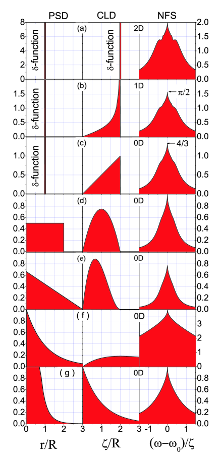
Figure 10: Size distributions (left column), thickness distributions (middle), and NFS lineshapes (right) for 2D layer (a), 1D wires (b), uniformly-sized spheres (c), spheres with rectangular (d), triangular (e), exponential (f) size distributions and with the size distribution of the form $F(r)=(R/r^{2}+2/r)\exp(-2r/R)$ (g). In (a) $R$ is the layer half-thickness, elsewhere $R$ is the average radius of sphere or wire.

13 3.7. Thickness distribution and lineshape for filaments or wires of the radius $R$

In the particulate matter, owing to the distribution of the chord lengths the theoretical NFS lineshape acquires the forms shown in the last columns of Fig. 10. In first and second columns, the PSD and CLD are shown, respectively. The hypergeometric function of Eq.(11) is reproduced in (a) in the same raw with the uniform thickness layer PSD and CLD, both represented by $\delta$-functions. The second raw (b) correspond to the filaments or wires of uniform radius. They are placed into the plane perpendicular to the beam direction, therefore, their CLD correspond to the distribution of the chord lengths $\zeta$ of the discs in 2D. For a disc of the size $2R$ using the running impact parameter $b$ we can express $\zeta=2\sqrt{R^{2}-b^{2}}$and $b=\sqrt{R^{2}-\zeta^{2}/4}$. Similarly to thickness distribution [3] the CLD $d(\zeta)$ can be found from the relationship $d(\zeta)=dS/S$. Here $dS$ is the relative part of the sample having thickness $\zeta.$ Therefore, the disc CLD is $d(\zeta)=$ $S^{-1}(dS/d\zeta)=b^{-1}\left|db/d\zeta\right|=\zeta(4R)^{-1}(R^{2}-\zeta^{2}/4)^{-\frac{1}{2}}$. The lineshape can be obtained through integration of the disc CLD with the right-hand side of the Eq. (11) and $\zeta$ from the Eq. (10):

$${\displaystyle\int\limits_{0}^{2R}}\frac{\left[1-h_{\frac{3}{2}}\left(-\frac{4\zeta^{2}}{\pi^{2}\omega^{2}}\right)\right]}{(R^{2}-\zeta^{2}/4)^{\frac{1}{2}}}\frac{\zeta^{2}d\zeta}{4R}=\frac{\pi R}{2}\left[\allowbreak 1-h_{2}\left(-\frac{16R^{2}}{\pi^{2}\omega^{2}}\right)\right]$$ (15)

The last but one argument of the hypergeometric function is used as a subscript in our notation $h_{2}(x)$ $\equiv$ ${}_{2}\digamma_{3}[\{\frac{1}{3},\frac{3}{4}\},\{\frac{1}{2},1,2\},x]$.

14 3.8. Lineshape for spherical particles of the radius $R$

In the third row (c) and in rows below (d,e,f) of Fig.10, the scattering matter consist of 0D-objects, i.e., spherical particles. In (c) all the particles have spherical shape and constant radius. The RTD function coincides with $d(\zeta)$ when the particles are distributed over the plane surface $S$ in such a way that shadowing of one particle by another is excluded. Again, we have the impact distance $b=\sqrt{R^{2}-\zeta^{2}/4}$, however, $dS/S$ is now $(\pi R^{2})^{-1}(2\pi bdb/d\zeta)=\zeta/2R^{2}(0<\zeta<2R)$. Then

$${\displaystyle\int\limits_{0}^{2R}}\left[1-h_{\frac{3}{2}}\left(-\frac{4\zeta^{2}}{\pi^{2}\omega^{2}}\right)\right]\frac{\zeta^{2}d\zeta}{2R^{2}}=\frac{4R}{3}\left[\allowbreak 1-h_{\frac{5}{2}}\left(-\frac{16R^{2}}{\pi^{2}\omega^{2}}\right)\right]$$ (16)

Similarly to Eqs.(11,15) the last but one argument is used as a subscript $h_{\frac{5}{2}}(x)\equiv$ ${}_{2}\digamma_{3}[\{\frac{1}{3},\frac{3}{4}\},\{\frac{1}{2},1,\frac{5}{2}\},x]$.

15 3.9. Lineshapes generated by several characteristic particle size distributions

Assuming the spherical particles to have some distribution in size we observe (Fig. 10 (d, e) that the PSD’s of rectangular and triangular shape result in the lineshapes with smeared shoulders. No shoulders can be apperceived for the cases (f) and (g), related to exponential PSD and exponential CLD, respectively. All the PSD’s except (g) are normalized to have the same area and the same mean particle size $\langle r\rangle=R$. The CLD’s $d(\zeta)$ are derived from PSD’s $F(r)$ using the formula[16]:

$$d(\zeta)=\frac{\zeta}{2R^{2}}{\displaystyle\int\limits_{\zeta/2}^{\infty}}F(r)dr$$ (17)

In case of exponential PSD (f), i.e., $F(r)=(1/R)\exp(-r/R)$, the Eq.(17) results in the CLD $d(\zeta)=(\zeta/4R^{2})\exp(-\zeta/2R)$. Integrating this $d(\zeta)$ with the right-hand side of the Eq. (11) and $\zeta$ from the Eq. (10) we obtain the spectral lineshape

$${\displaystyle\int\limits_{0}^{\infty}}\left[1-h_{\frac{3}{2}}\left(-\frac{4\zeta^{2}}{\pi^{2}\omega^{2}}\right)\right]\frac{\zeta^{2}\exp(-\zeta/2R)d\zeta}{4R^{2}}=$$

$$=4R\allowbreak\left[1+\frac{2\sqrt{\pi}R\sin(3\Phi/2)}{\omega(\pi^{2}+\frac{64R^{2}}{\omega^{2}})^{\frac{3}{4}}}-\frac{\sqrt{\pi}\cos(\Phi/2)}{(\pi^{2}+\frac{64R^{2}}{\omega^{2}})^{\frac{1}{4}}}\right]$$ (18)

Here $\Phi=\arctan(8R/\pi\omega)$. As far as the relative weight of smaller particles increases from top to bottom of Fig. 10 the shoulders became less articulated and disappear in (f).

Further increase in the fraction of small particles is the case (g) related to divergence of $F(r)$ at $r\longrightarrow 0$. Substituting $F(r)=(r/R^{2}+2/r)\exp(-2r/R)$ into Eq. 17 we obtain the simple exponential CLD $d(\zeta)=R^{-1}\exp(-\zeta/2R)$, which is broadly found among the natural particulate materials. Since this $F(r)$ has a singularity at $r\longrightarrow 0$ , such a PSD cannot be normalized in the same way as the PSD’s (d), (e) and (f). However, $d(\zeta)$ can be normalized in a usual way ${\textstyle\int}d(r)dr=1$ with the average chord length $\langle\zeta\rangle=R$. Many kinds of complex interfacial media exhibit the exponential CLD. Numerous examples of the exponential CLD’s were demonstrated [17] among the porous borosilicate glasses, heterogeneous catalysts, cements etc. Also, if we mix the hard spherical particles of non-resonant media with soft resonant background we expect an exponential CLD for the resonant component[18]. The absorbers for NFS are frequently prepared through mixing the resonant nanoparticles (e.g., ⁵⁷Fe₂O₃ in [11]) with larger particles of non-resonant filling medium.

The divergence of $F(r)$ at small particle radius ($r\longrightarrow 0$) is so strong that the integral ${\textstyle\int}F(r)dr$ is also divergent. This nonitegrability implies that the spherical shape assumption (Eq. 17) is rather unphysical for the exponential CLD $d(\zeta)=(1/R)\exp(-\zeta/R)$ [16]. Indeed, this $d(\zeta)$ is the chord length distribution in the background material filling the interstices between spheres[18]. Integrating this $d(\zeta)$ with the right-hand side of the Eq. (11) and $\zeta$ from the Eq. (10) we obtain the lineshape of such a background:

$${\displaystyle\int\limits_{0}^{\infty}}\left[1-h_{\frac{3}{2}}\left(-\frac{4\zeta^{2}}{\pi^{2}\omega^{2}}\right)\right]\frac{e^{-\frac{\zeta}{R}}\zeta d\zeta}{R}=R\left[\allowbreak 1-\frac{\sqrt{\pi}\cos(\phi/2)}{(\pi^{2}+\frac{16R^{2}}{\omega^{2}})^{\frac{1}{4}}}\right]$$ (19)

Here $\phi=\arctan(4R/\pi\omega).$

16 3.10. Determination of the particle size distribution parameters

The Eqs. (11), (16), (18) and (19) were employed to fit the upper-frequency line from the $\exp(\tau)$-sharpened spectrum of Fig. 8. First, assuming a layer of uniform thickness the Eq.(11) was used. Fitting the line at 185 MHz with the hypergeometric function $1-h_{3/2}\left(-4\zeta^{2}/\pi^{2}\omega^{2}\right)$ has resulted in the value of the dimensionless thickness $\zeta_{0}=4.36$ (Fig.11). According to the Eq.(9) the total Mossbauer thickness is $\zeta_{0}^{\text{tot}}=4\zeta_{0}\simeq 17.4$. This is very close to the value of $\zeta^{\text{tot}}=19.5$ obtained above in time domain through fitting the NFS spectrum as a whole.

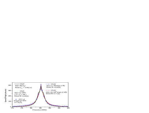
Figure 11: The section from 170 MHz to 200 MHz of the quantum beat frequency spectra (square-shaped symbols) fitted with the right-hand expressions in Eqs. (18) and (19) (lines).

Turning from dimensionless $\zeta^{\text{tot}}$ to metric units of $z=\zeta^{\text{tot}}/\pi\mu^{\text{tot}}$ and using $\mu^{\text{tot}}=\sigma_{0}\rho f_{\text{LM}}\eta$ with $\sigma_{0}=2.56\cdot 10^{-18}$ cm², $\rho=3.96\cdot 10^{22}$ cm^-3, $f_{\text{LM}}=0.8$, $\eta=0.0212$, we obtain the total coefficient of nuclear absorption for unenriched hematite $\mu^{\text{tot}}=0.172$ $\mu$m^-1. From the Eq.(9) the layer thickness $z_{0}$ that corresponds to $\zeta_{0}^{\text{tot}}=17.4$ is (shown by the position of $\delta$-function in Fig.12):

$$z_{0}=4\zeta_{0}^{\text{tot}}/\pi\mu^{\text{tot}}=16\zeta_{0}/\pi\mu^{\text{tot}}=129\mu m$$ (20)

Figure 12: Chord length distributions $d(z)$ used to fit the highest-frequency line of the NFS Fourier spectra of Fig.8 at the values of the dimensionless parameters: $\zeta_{0}=4.36$ in $d(\zeta)=\delta(\zeta-\zeta_{0})$, $R=2.89$ in $d(\zeta)=\frac{\zeta}{2R^{2}}$, $R=2.38$ in $d(\zeta)=\frac{1}{R}e^{-\frac{\zeta}{R}}$ and $R=0.82$ in $d(\zeta)=\frac{\zeta}{4R^{2}}e^{-\frac{\zeta}{2R}}$.

Certainly, a sample formed by the particles of Fe₂O₃ of a finite size appears worthy of a better characterization. Assuming all the particles having the same size and spheric shape, we can estimate the radius of particle using Eq.(16). The fit results in the value of $R$ of $2.84$. In this model, the thickness is distributed linearly between $0$ and $2R$ (Fig.12). The particle diameter of 168 $\mu$m is larger by 30% than uniform thickness $z_{0}$ from the Eq.(20). Here again as in Eq.(20) the hematite-specific length factor $r_{0}=16/\pi\mu^{\text{tot}}=29.61\mu$m brings the diameter $2Rr_{0}$ to the metric scale. The goodness of fit becomes better when we proceed from uniform layer to the ball-shaped particles, namely, the coefficient of determination $\mathbf{R}^{\mathrm{2}}$ increases from 0.991 to 0.994. Although the increase is not large, the usage of the $\mathbf{R}^{\mathrm{2}}-$coefficient is justified at comparing the goodness of fit for different models because all of our models use the same number of parameters.

Among the models with distributions of particle sizes two models were tested, according to the Eqs.(18,19). Goodness of fit was slightly better for the first (Eq. 18, $\mathbf{R}^{\mathrm{2}}=0.995$) than for the second (Eq. 19, $\mathbf{R}^{\mathrm{2}}=0.993$). Corresponding chord lengths distributions are also shown in Fig.12. The quality of fit between these two distributions is not much different, the values of fitted radius $R$ for the CLD of spheres is nearly 3 times smaller than the value of $R$ for the CLD of the background between spheres. In the chord length range $38$ $\mu$m $<z<260$ $\mu$m the CLD density for spheres is larger than the CLD density for the background. Opposite is true elsewhere. Clearly, the excess in the range $38$ $\mu$m $<z<260$ $\mu$m is compensated by the contribution of large particles, although their CLD density above $260$ $\mu$m is below 5%. In this sense, the chord length of $260$ $\mu$m is the characteristic length invariant of the fitting model employed. Interestingly, this ”inhomogeneous” length is twice larger than the value obtained in Eq.(20) for the homogeneous layer.

17 4. Conclusions

Starting from several characteristic states of scattering matter (foil, filaments, particles) we have solved the problem of determination of corresponding spectral lineshape parameters for the nuclear forward scattering Fourier spectra. The method is useful in the range of thicknesses where quantum beat envelopes vary slowly compared to the quantum beats themselves. In the frequency domain, we are able to predict the lineshapes determined by Fourier transforms of the envelopes. These lineshapes are of polaritonic nature since they originate from the energy exchange between the radiation field and nuclear excitation. Both the radiation and the nuclear currents are the components of the compound quasiparticle termed the nuclear exciton polariton. From these lineshapes we derive the parameters of resonant thickness distribution.

When fragments of resonant and nonresonant media are interleaved so that the standard methods of neutron or x-ray small-angle scattering (SAS) cannot distinguish between fragments of similar electronic or nuclear density, the proposed technique would be able to resolve between them. Therefore, if a fraction of the ⁵⁷Fe-containing ’particles’ cannot be detached from a ’membrane’, then the methods of SAS would produce the information on the density distribution in the system ’particles+membrane’. Separately, the particles subsystem can be studied by NFS without membrane detaching that is most frequently unrealizable. Supported catalysts present the archetype of future applications.

Practical applications of the proposed analysis are quite feasible already at the existing beamlines of the synchrotron rings of third generation. The sampling frequency does not require any improvements, because it can be needed only for very thick samples. The time resolution of the avalanche photodiode detectors ($\sim$0.1 ns) correspond closely to the currently applied sampling frequency. Much more important for the proposed technique would be the improvements in the high-rate characteristics of the detectors and in the span of the time window between electron bunches. Change from multiple-bunch to single-bunch regime is crucial to achieve a better cutoff time $\tau_{\max}$. Also, with the advent of novel avalanche detectors and detector arrays [19, 20] the region of missing data at small $\tau$ might be shortened.

Inverse problem of finding the characteristic parameters of the particle chord length distribution from the polaritonic lineshapes would be possible to solve using regularization methods. Then, not only PSD parameters could be refined starting from one or another hypothesis, but also the full PSD profiles could be reconstructed.

This work was supported by RFBR-JSPS Grant 07-02-91201.

References

- [1] \NameKagan Yu., Afanas’ev A.M., Kohn V.G. \REVIEWJ. Phys. C121979615.
- [2] \NameFeigin L.A. Svergun D.I. \BookStructural Analysis by Small-Angle X-ray and Neutron Scattering \EditorGeorge W. Taylor \PublPlenum Press, New York \Year1987 \Page44.
- [3] \NameBausk N.V., Erenburg S.B. , Mazalov L.N. \REVIEWJ. Synchrotron Rad. 61999 268-270.
- [4] \Name Gille W. \REVIEWEur. Phys. J. B. 172000 371-383.
- [5] \Name Gerdau E., Rüffer R., Hollatz R., and Hannon J. P. \REVIEWPhys. Rev. Lett. 571986 1141.
- [6] \NameHastings J.B., Siddons D.P., van Bürck U., Hollatz R., Bergmann U. \REVIEWPhys. Rev. Lett. 661991 770.
- [7] \Namevan Bürck U., Siddons D.P., Hastings J.B., Bergmann U. Hollatz R. \REVIEWPhys. Rev. B. 461992 6207.
- [8] \NameSmirnov G. V. \REVIEWHyperfine Interact. 97/981996551.
- [9] \Namevan Bürck U. \REVIEWHyperfine Interact. 123/1241999483-509.
- [10] \NameShvyd’ko Yu. V. , van Bürck U. ,Potzel W. ,Schindelmann P.,Gerdau E.,Leupold O.,Metge J.,Rüter H.D., and Smirnov G.V. \REVIEW, Phys. Rev. B 571998 3552-3561
- [11] \NameRykov A.I., Rykov I. A., Nomura K., Zhang X. \REVIEWHyperfine Interact. 163200529-56.
- [12] \NameSmirnov G. V. \REVIEWHyperfine Interact. 123/124199931-77.
- [13] \NameShvyd’ko Yu. V. , van Bürck U. \REVIEWHyperfine Interact. 123/1241999511-527.
- [14] \NameSmirnov G.V., van Bürck U., Arthur G., Brown G.S., Chumakov A.I., Baron A.Q.R., Petry W., Ruby S.L. \REVIEWPhys. Rev. A762007 043811..
- [15] \NameKohn V.G. Smirnov G.V. \REVIEWPhys. Rev. B762007 104438..
- [16] \NameOlson G.L., Miller D.S., Larsen E.W. Morel J.E. \REVIEWJ. Quantitative Specroscopy and Radiative Transfer 1012006269-283.
- [17] \NameLevitz P., Tchoubar D. \REVIEWJ. Phys. I France 21992771-790.
- [18] \NameOlson G.L. \REVIEWAnnals Nucl. Energy 3520082150-2155.
- [19] \Name Kishimoto S., Yoda Y., Seto S., Kitao S., Kobayashi Y., Haruki R. Harami T. \REVIEWNuclear Instruments and Methods in Physics Research A 5132003193.
- [20] \Name Baron A.Q.R., Kishimoto S., Morse J., Rigal J.-M. \REVIEWJ. Synchrotron Rad. 132006 131-142.