Optimal time-dependent polarized current pattern for fast domain wall propagation in nanowires: Exact solutions for biaxial and uniaxial anisotropies

Abstract

One of the important issues in nanomagnetism is to lower the current needed for a technologically useful domain wall (DW) propagation speed. Based on the modified Landau-Lifshitz-Gilbert (LLG) equation with both Slonczewski spin-transfer torque and the field-like torque, we derive the optimal spin current pattern for fast DW propagation along nanowires. Under such conditions, the DW velocity in biaxial wires can be enhanced as much as ten times compared to the velocities achieved in experiments so far. Moreover, the fast variation of spin polarization can help DW depinning. Possible experimental realizations are discussed.

Introduction$\emph{.}{\LARGE-}$Fast magnetic domain wall (DW) propagation along nanowires by means of electrical currents is presently under intensive study in nano-magnetism, both experimentally Parkin ; Yamaguchi ; Klaui1 ; Erskine1 ; Hayashi and theoretically Tatara1 ; Barnes ; Brataas . In addition to the technological interest such as race track memory Parkin , DW dynamics is also an interesting fundamental problem. The dynamics of a single DW can be qualitatively understood from one-dimensional (1D) analytical models Walker ; Slonczewski ; Thiaville that predict a rigid-body propagation below the Walker breakdown and an oscillatory motion above it Walker ; xrw1 . The latter process is connected with a series of complicated cyclic transformations of DW structure and a drastic reduction of the average DW velocity. The Walker limit is thus the maximum velocity at which DW can propagate in magnetic nanowires without changing its inner structure. From a technological point of view, such a limit seems to represent a major obstacle since the fidelity of data transmission may depend on preserving the DW structure while the utility requires speeding up the DW velocity adequately. Various efforts have been made to overcome this limit through geometry design. For instance, Lewis et al. Lewis proposed a “chirality filter” consisting of a cross-shaped trap to preserve the DW structure. Yan et al. Yan demonstrated the removal of Walker limit via a micromagnetic study on the current-induced DW motion in cylindrical Permalloy nanowires. In this Letter we investigate other ways to substantially increase the DW velocity avoiding the Walker breakdown.

A DW propagates under a spin-polarized current through angular momentum transfer from conduction electrons to the local magnetization, known as the spin transfer torque (STT) Slon , which is different from magnetic field driven DW propagation originated from the energy dissipation xrw1 ; Sun . Generally, two types of spin torques are considered: the Slonczewski torque Slon ($a-$term) $\mathbf{T}_{\text{a}}=-\gamma\frac{a_{J}}{M_{s}}\mathbf{M}\times\left(\mathbf{M}\times\mathbf{s}\right)$ and the field-like torque Heide ; szhang2 ($b-$term) $\mathbf{T}_{\text{b}}=-\gamma b_{J}\mathbf{M}\times\mathbf{s}$, where $\gamma=\left|e\right|/m_{e}$, $\mathbf{M}$, $M_{s}=\left|\mathbf{M}\right|$, and $\mathbf{s}$ are the the gyromagnetic ratio, magnetization of the magnet, the saturation magnetization, and the spin polarization direction of itinerant electrons, respectively. $a_{J}$ and $b_{J}$ depend on current density $j_{e}$ and spin polarization $P$. Theory predicts Slon ; szhang2 that $a_{J}=Pj_{e}\hbar/2d\left|e\right|M_{s}$ and $b_{J}=\beta a_{J}$, where $d$ is the thickness of the free magnetic layer. $\beta$ is a small dimensionless parameter that describes the relative strength of the field-like torque to the Slonczewski torque. The value of $\beta$ is sensitive to the thickness of the free layer and the decay length of the transverse component of the spin accumulation inside the free layer as discussed in Ref. szhang2 . The typical value of $\beta$ ranges from $0$ to $0.5$ szhang2 ; Stiles . In the conventional case of current along the nanowire with biaxial magnetic anisotropy, the $a-$term is incapable of generating a sustained DW motion, except for a very large current, while the $b-$term can drive a DW to propagate Tatara1 . Unfortunately, the $b-$term is usually much smaller than $a-$term Erskine1 ; Hayashi . A large current density is needed in order to reach a technologically useful DW propagation velocity Parkin , but the associated Joule heating and DW structure collapse could affect device performance. We show that the problem can be solved if one uses an optimal polarized current pattern.

In this Letter, our focus is on the optimal spin-polarized electric current pattern for fast DW propagation along nanowires. For usual magnetic materials, our theoretical results show that the DW velocity can be enhanced by as large as ten times in comparison with DW velocity driven by the conventional constant current in existing experiments. Moreover, the ultrafast change of spin polarization can be used to de-pin a DW.

Model$\emph{.}{\LARGE-}$ The internal magnetic energy of a nanowire can be formulated as

$$U\left[\mathbf{M}\right]=\int d^{3}x\Bigl{(}\frac{J}{2}\left[\left(\nabla\theta\right)^{2}+\sin^{2}\theta\left(\nabla\phi\right)^{2}\right]+w\left(\theta,\phi\right)\Bigr{)},$$ (1)

where $\theta$ and $\phi$ are the polar angle and azimuthal angle of the local magnetization $\mathbf{m=M}/M_{s},$ respectively. $J$ and $w$ are the exchange energy constant and energy density due to all kinds of anisotropies, respectively. The dynamics of $\mathbf{M}$ is governed by the LLG equation Gilbert :

$$\frac{\partial\mathbf{M}}{\partial t}=-\gamma\mathbf{M}\times\mathbf{H}_{eff}+\frac{\alpha}{M_{s}}\mathbf{M}\times\frac{\partial\mathbf{M}}{\partial t}+\mathbf{T}_{\text{STT}},$$ (2)

here $\mathbf{H}_{eff}=-\frac{1}{\mu_{0}}\delta U/\delta\mathbf{M}$ is the effective magnetic field and $\alpha$ is the phenomenological Gilbert damping constant Gilbert . $\mathbf{T}_{\text{STT}}$ is the STT with both the Slonczewski-type and the field-like terms.

Biaxial anisotropy$\emph{.}{\LARGE-}$Considering a biaxial anisotropy $w\left(\theta,\phi\right)=-\frac{K}{2}m_{z}^{2}+\frac{K_{\perp}}{2}m_{x}^{2}$ with the easy axis along $\hat{z}$ direction and the hard axis along $\hat{x}$ direction, the effective field takes a form of $\mathbf{H}_{eff}=\frac{1}{\mu_{0}M_{s}}\left(Km_{z}\hat{z}-K_{\perp}m_{x}\hat{x}\right)+\frac{J}{\mu_{0}M_{s}^{2}}\frac{\partial^{2}\mathbf{M}}{\partial z^{2}}.$ Here $K$ and $K_{\perp}$ describe energetic anisotropies along easy $\hat{z}$ axis and hard $\hat{x}$ axis, respectively. We assume that all local spins lie in a fixed plane called DW plane, i.e., $\phi\left(z,t\right)=\phi\left(t\right),$ which should be checked self-consistently late. In the spherical coordinates, Eq. (2) becomes

$$\dot{\theta}+\alpha\sin\theta\dot{\phi} = \gamma a_{J}\left(s_{\theta}+\beta s_{\phi}\right)+\frac{\gamma K_{\perp}}{2\mu_{0}M_{s}}\sin\theta\sin 2\phi,$$

$$\sin\theta\dot{\phi}-\alpha\dot{\theta} = \gamma a_{J}\left(s_{\phi}-\beta s_{\theta}\right)$$ (4)

$$-\gamma\frac{J\frac{\partial^{2}\theta}{\partial z^{2}}-\frac{\sin 2\theta}{2}\left(K+K_{\perp}\cos^{2}\phi\right)}{\mu_{0}M_{s}},$$

where $s_{r},$ $s_{\theta},$ and $s_{\phi}$ are three components of unit spin vector $\mathbf{s}$ in spherical coordinates. The DW profile satisfies $J\frac{\partial^{2}\theta}{\partial z^{2}}-\frac{\sin 2\theta}{2}\left(K+K_{\perp}\cos^{2}\phi\right)=0$ with boundary condition of $\theta=0$ and $\pi$ at distance. One obtains the famous Walker’s DW motion profile $\tan\frac{\theta}{2}=\exp\left(\frac{z-X\left(t\right)}{\Delta}\right),$ in which $X\left(t\right)$ is the position of the DW center and $\Delta=\sqrt{\frac{J}{K+K_{\perp}\cos^{2}\phi}}$ is DW width resulting from the balance of anisotropy energy and exchange energy Walker . These assumptions are valid under sufficiently low current density which will be demonstrated later. Substituting this DW profile into Eqs. (LABEL:LLG0) and (4), we have

$$-\frac{\dot{X}}{\Delta}+\alpha\dot{\phi} = \gamma\frac{a_{J}\left(s_{\theta}+\beta s_{\phi}\right)}{\sin\theta}+\frac{\gamma K_{\perp}}{2\mu_{0}M_{s}}\sin 2\phi,$$ (5)

$$\alpha\frac{\dot{X}}{\Delta}+\dot{\phi} = \gamma\frac{a_{J}\left(s_{\phi}-\beta s_{\theta}\right)}{\sin\theta}.$$ (6)

For a given DW motion, term $s_{\phi}-\beta s_{\theta}$ should be as large as possible in order to lower the needed current density. Meanwhile, considering identity $\left(s_{\phi}-\beta s_{\theta}\right)^{2}+$ $\left(s_{\theta}+\beta s_{\phi}\right)^{2}=\left(1+\beta^{2}\right)\left(1-s_{r}^{2}\right),$ we choose

$$s_{r}=0,\text{ }s_{\theta}=\cos\eta,\text{ }s_{\phi}=\sin\eta,$$ (7)

with optimization parameter $\eta$.

To ensure the spatial-independence of $\dot{X}$ and $\phi,$ the above equations require $a_{J}$ to be proportional to $\sin\theta,$ so we let $a_{J}=A_{J}\sin\theta=A_{J}\sec$h$\left(\frac{z-X\left(t\right)}{\Delta}\right)$ with a constant $A_{J}.$ Thus we have

$$\dot{X} = \gamma\Delta\frac{\alpha a_{J}^{\prime}-b_{J}^{\prime}}{1+\alpha^{2}}-\Delta\frac{\gamma K_{\perp}}{2\mu_{0}M_{s}\left(1+\alpha^{2}\right)}\sin 2\phi,$$ (8)

$$\dot{\phi} = \gamma\frac{a_{J}^{\prime}+\alpha b_{J}^{\prime}}{1+\alpha^{2}}+\frac{\alpha\gamma K_{\perp}}{2\mu_{0}M_{s}\left(1+\alpha^{2}\right)}\sin 2\phi,$$ (9)

which describe the DW propagation and the DW plane precession. Here $a_{J}^{\prime}\left(\eta\right)=A_{J}\left(\sin\eta-\beta\cos\eta\right)$ and $b_{J}^{\prime}\left(\eta\right)=A_{J}\left(\cos\eta+\beta\sin\eta\right)$. The DW width is time-independent when the DW undergoes a rigid-body propagation with $\phi\left(t\right)=\phi_{0}=$constant. In general, DW width $\Delta$ depends on the time through time-dependence of $\phi.$ The exact rigid-body solutions constitute

$$\frac{\alpha K_{\perp}}{2\mu_{0}M_{s}}\sin 2\phi_{0}\left(\eta\right) = -\left(a_{J}^{\prime}+\alpha b_{J}^{\prime}\right),$$ (10)

$$\Delta\left(\eta\right) = \sqrt{\frac{J}{K+K_{\perp}\cos^{2}\phi_{0}\left(\eta\right)}},$$ (11)

$$\dot{X}\left(\eta\right) = \gamma\frac{a_{J}^{\prime}}{\alpha}\Delta\left(\eta\right).$$ (12)

The spin current pattern is then described by $\eta.$ Different value leads to different canted angle, DW width and propagation velocity. It is straightforward to show that the assumption of rigid-body motion always holds under condition $A_{J}\sqrt{\left(1+\alpha^{2}\right)\left(1+\beta^{2}\right)}\leq\frac{\alpha K_{\perp}}{2\mu_{0}M_{s}}.$

Before finding the optimized spin current pattern for maximal velocity, let’s first consider two special cases. The conventional case in the existing experiments Fert ; Boone is the constant current density with electron spin polarization along $z-$axis, i.e., $s_{\theta}=-\sin\theta$ and $s_{\phi}=0,$ which gives the velocity $u_{1}=\gamma\frac{\beta A_{J}}{\alpha}\Delta\left(\pi\right).$ It again shows that Slonczewski torque is incapable of generating sustained DW propagation while the field-like torque can. But the velocity is rather small since $\beta\ll 1$ in usual materials. However, the DW velocity can be greatly enhanced if $a-$term is involved. This is the case of $\eta=\frac{\pi}{2}.$ It gives the velocity $u_{2}=\gamma\frac{A_{J}}{\alpha}\Delta\left(\frac{\pi}{2}\right).$ In typical materials Stiles , $\beta\sim 0.1,$ so the velocity is 10 times lager than $u_{1}.$ One can see that DW propagation velocity is greatly enhanced under a modification of the spin polarization and locally minimized current density pattern.

The maximal velocity $\dot{X}_{\max}=\dot{X}\left(\eta^{\ast}\right)$ at the optimal parameter $\eta^{\ast}$ can be found through exact numerical calculations although a closed analytic form is difficult to obtain due to the complexity of Eqs. (10), (11), and (12). Factor $\lambda=\dot{X}_{\max}/u_{1}=\frac{\sin\eta^{\ast}-\beta\cos\eta^{\ast}}{\beta}\frac{\Delta\left(\eta^{\ast}\right)}{\Delta\left(\pi\right)}$ measures the velocity enhancement. Fig. 1a is the $\beta^{-1}$ dependence of $\lambda$ for various damping coefficients and typical magnetic parameters. It is approximately linear, and insensitive to damping parameter $\alpha$. Fig. 1b is the plot of spatial distribution of $s_{x},$ $s_{y},$ $s_{z}$ and $a_{J}$ for the optimized spin current pattern around DW center. We note that $s_{x},$ $s_{y},$ and $s_{z}$ vary only near the DW center, and reach fixed values away from the DW. A large perpendicular component $s_{y}$ is required to achieve large DW velocity. The reason is that perpendicular spin component induces a large effective field $\mathbf{H}_{a}=\frac{a_{J}}{M_{s}}\mathbf{M}\times\mathbf{s.}$ Thus the DW moves under the Slonczewski torque with a large component along wire axis. This finding is consistent with recent micromagnetic simulations Khvalkovskiy showing that the DW velocity can be greatly increased by applying perpendicular spin polarizations. It is also very interesting that locally minimized current density $a_{J}$ is finite only near DW center while it becomes zero at distance, which should greatly lower the energy consumption.

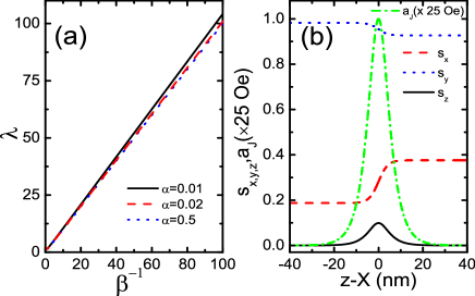
Figure 1: (Color online) (a) DW velocity enhancement factor $\lambda$ versus $\beta^{-1}$ at different damping coefficients $\alpha=0.01,0.02$ and $0.5$. (b) The spatial distribution of $x,y,z$ components of the optimal spin polarization pattern and current density pattern for maximal DW velocity under $\alpha=0.01$ and $\beta=0.1$. The other parameters are using the materials parameters of Permalloy: $M_{s}=8.6\times 10^{5}$ A/m, $J=1.3\times 10^{-11}$ J/m, $K=500$ J/m³, $K_{\perp}=8\times 10^{5}$ J/m³ Parkin , and a reasonable value $A_{J}=25$ Oe according to Ref. Khvalkovskiy .

Depinning$\emph{.}{\LARGE-}$Besides the advantage of markedly speeding up the DW velocity, our time-dependent spin current pattern also implies a possible way to improve the efficiency of DW motion against the pinning effect. The argument is attributed to an additional force on the wall due to a fast changing spin direction. It is convenient for us to treat DW as a quasiparticle Doring with mass $m_{\text{w}}=\frac{2S\mu_{0}^{2}M_{s}^{2}}{\Delta\gamma^{2}K_{\perp}}$ Kruger ; Bocklage when we deal with the effect of pinning. Here $S$ is the cross section of the wire. The pinning force $F_{\text{pin}}=-\frac{dE}{dX}$ is expressed by the pinning potential $E$ and the position $X$ of the wall. Thus for small $\phi,$ Eqs. (8) and (9) can be simply decoupled and result in

$$\frac{F}{m_{\text{w}}} = \ddot{X}=\frac{\alpha\gamma K_{\perp}}{\left(1+\alpha^{2}\right)\mu_{0}M_{s}}\dot{X}-\frac{1}{m_{\text{w}}}\frac{dE}{dX}$$ (13)

$$-\Delta\frac{\gamma^{2}K_{\perp}}{\mu_{0}M_{s}}\frac{a_{J}^{\prime}}{1+\alpha^{2}}+\gamma\Delta\frac{a_{J}^{\prime}+\alpha b_{J}^{\prime}}{1+\alpha^{2}}\dot{\eta},$$

where the temporal variation of DW width is neglected. The contributions of current-induced acceleration are the last two terms. In usual setup ($\mathbf{s}$ along the wire axis), the depinning acceleration due to STT is $\ddot{X}_{\text{sp}}=-\Delta\frac{\gamma^{2}K_{\perp}}{\mu_{0}M_{s}}\frac{\beta A_{J}}{1+\alpha^{2}}$ Bocklage . Thus, one can observe that our optimal spin current pattern provides a higher depinning acceleration by $10$ times for the current density part since parameter $\beta$ is typically around 0.1 Stiles . The force $F$ on the wall does not only depend on the current density but also on the time derivative of spin direction. The switching-time dependence of current-induced depinning follows the last term in Eq. (13). For a fast changing current, i.e., spin variation rate $\tau\ll\frac{\mu_{0}M_{s}}{\gamma K_{\perp}}\sim 10^{-12}$ s, the contribution of the time derivative term will be significant. The novelty and importance of our proposal are embodied in the nature of ultrafast switching-time of spin degree of freedom. It makes a main difference from the DW depinning due to current density’s rise time Bocklage which is limited by the intrinsic response time of circuit Heyne .

Uniaxial anisotropy$\emph{.}{\LARGE-}$Let $K_{\perp}=0,$ Eqs. (8) and (9) result in

$$\dot{X}^{2}+\dot{\phi}^{2}\Delta^{2}=\frac{\gamma^{2}\Delta^{2}A_{J}^{2}}{1+\alpha^{2}}\left(1+\beta^{2}\right),$$ (14)

with DW width parameter $\Delta=\sqrt{J/K}.$

Thus, the largest possible DW propagation velocity is $\dot{X}_{\max}=\gamma A_{J}\sqrt{\left(1+\beta^{2}\right)/\left(1+\alpha^{2}\right)}\Delta.$ The conventional polarization Fert ; Boone gives the DW velocity $u=\gamma A_{J}\frac{1+\alpha\beta}{1+\alpha^{2}}\Delta.$ As a result, the DW velocity is enhanced under the optimal spin current pattern by a factor of $\dot{X}_{\max}/u=$ $\sqrt{1+\left(\frac{\alpha-\beta}{1+\alpha\beta}\right)^{2}}$. We note that the enhancement is not so large in the uniaxial wire since both $\alpha$ and $\beta$ are far less than $1$ in usual magnetic materials xrw2 . The physical reason lies in that $a-$term is capable of generating a sustained DW motion in uniaxial wire, which is different from biaxial case.

Discussion$\emph{.}{\LARGE-}$Although the optimal spin current pattern for maximum DW velocity is found, it is still an experimental challenge to generate a temporally and spatially varying spin polarized current. Interestingly enough, a very recent experiment used spin-polarized current perpendicular to a nanowire to manipulate DW motion Boone . There are now at least two types of current patterns realizable. The hope is that our capable experimentalists can one day generate any designed current pattern. Indeed, there are many theoretical proposals for generating a designed current pattern. Tao et al. Tao and Delgado et al. Delgado have proposed to use magnetic scanning tunneling microscopic (STM) tip above a magnetic nanowire to produce localized spin-polarized current. Experimentally, the control of spin-polarized current in a STM by single-atom transfer was demonstrated very recently by Ziegler et al Ziegler . In summary, our proposed optimal spin current patterns are difficult to generate now, but their existence does not violate any fundamental laws and principles. Our results and calculations will be relevant to experiments when the generation of an arbitrary spin-polarized current pattern becomes true.

In the above discussions, the spin pumping effect on the DW motion is neglected because the DW-motion induced current is zero in biaxial wire since there is no DW plane precession xrw3 below Walker breakdown and it is much smaller than the applied external spin-polarized current in uniaxial wire. According to Ref. Duine , the maximum DW-motion generated electric current density in uniaxial wire is $\left\langle j_{z}\right\rangle=\frac{\hslash}{eL}\left(\sigma_{\uparrow}-\sigma_{\downarrow}\right)\frac{\dot{X}_{\max}}{\Delta},$ where $L$ is the length of the nanowire, $\sigma_{\uparrow}$ and $\sigma_{\downarrow}$ denote the conductivities of the majority and minority electrons. In the experiments of Beach et al. Erskine1 , $L\sim 40$ $\mu$m, $\Delta\sim 20$ nm, and DW velocity $\dot{X}_{\max}\sim 40-100$ m/s. For a typical conductivity $\sigma_{\uparrow}\sim 10^{6}$ $\Omega^{-1}$m${}^{-1},$ one can find the pumped electric current density no more than $\left\langle j_{z}\right\rangle\sim 10^{5}-10^{6}$A/m${}^{2},$ which is much smaller than the typically applied current of the order of $10^{10}-10^{12}$A/m² in experiments Erskine1 .

Conclusion$\emph{.}{\LARGE-}$We propose an optimal spin current pattern for high DW propagation velocity in magnetic nanowires. In uniaxial wires this enhancement is of modest size, while in biaxial wires a factor of a few tens can be achieved. The nature of ultrafast switching-time of spin degree of freedom proves to be a novel way to improve the efficiency of DW motion against the pinning. We expect our proposal will stimulate and also possibly guide future experiments.

We thank Dr. X.J. Xia and Mr. W. Zhu for valuable discussions. This work is supported by Hong Kong RGC grants (#603007, 603508, 604109 and HKU10/CRF/08- HKUST17/CRF/08), and by Deutsche Forschungsgemeinschaft via SFB 689. Z.Z.S. thanks the Alexander von Humboldt Foundation (Germany) for a grant.

References

- (1) S.S.P. Parkin, M. Hayashi, and L. Thomas, Science 320, 190 (2008).
- (2) A. Yamaguchi, T. Ono, S. Nasu, K. Miyake, K. Mibu, and T. Shinjo, Phys. Rev. Lett. 92, 077205 (2004).
- (3) M. Kläui, P.O. Jubert, R. Allenspach, A. Bischof, J.A.C. Bland, G. Faini, U. Rüdiger, C.A.F. Vaz, L. Vila, and C. Vouille, Phys. Rev. Lett. 95, 026601 (2005).
- (4) G.S.D. Beach, C. Knutson, C. Nistor, M. Tsoi, and J.L. Erskine, Phys. Rev. Lett. 97, 057203 (2006).
- (5) M. Hayashi, L. Thomas, C. Rettner, R. Moriya, Y.B. Bazaliy, and S.S.P. Parkin, Phys. Rev. Lett. 98, 037204 (2007).
- (6) G. Tatara and H. Kohno, Phys. Rev. Lett. 92, 086601 (2004); S. Zhang and Z. Li, Phys. Rev. Lett. 93, 127204 (2004).
- (7) S.E. Barnes and S. Maekawa, Phys. Rev. Lett. 95, 107204 (2005).
- (8) K.M.D. Hals, A.K. Nguyen, and A. Brataas, Phys. Rev. Lett. 102, 256601 (2009).
- (9) N.L. Schryer and L.R. Walker, J. Appl. Phys. 45, 5406 (1974).
- (10) M.A. Slonczewski, Magnetic Domain Walls in Bubble Materials (Academic, New York, 1979).
- (11) A. Thiaville and Y. Nakatani, Spin Dynamics in Confined Magnetic Structures (Springer, Berlin, 2006), Vol III, p. 161.
- (12) X.R. Wang, P. Yan, J. Lu, and C. He, Ann. Phys. (N. Y.) 324, 1815 (2009); X.R. Wang, P. Yan, and J. Lu, Europhys. Lett. 86, 67001 (2009).
- (13) E.R. Lewis, D. Petit, A.V. Jausovec, L. O’Brien, D.E. Read, H.T. Zeng, and R.P. Cowburn, Phys. Rev. Lett. 102, 057209 (2009).
- (14) M. Yan, A. Kákay, S. Gliga, and R. Hertel, Phys. Rev. Lett. 104, 057201 (2010).
- (15) J. Slonczewski, J. Magn. Magn. Mater. 159, L1 (1996); L. Berger, Phys. Rev. B 54, 9353 (1996).
- (16) Z.Z. Sun and J. Schliemann, Phys. Rev. Lett. 104, 037206 (2010).
- (17) C. Heide, Phys. Rev. Lett. 87, 197201 (2001).
- (18) S. Zhang, P. M. Levy, and A. Fert, Phys. Rev. Lett. 88, 236601 (2002).
- (19) M.D. Stiles and A. Zangwill, Phys. Rev. B 66, 014407 (2002); K. Xia, P.J. Kelly, G.E.W. Bauer, A. Brataas, and I. Turek, Phys. Rev. B 65, 220401(R) (2002); M. Gmitra and J. Barnas, Phys. Rev. Lett. 96, 207205 (2006); M.A. Zimmler, B. Özyilmaz, W. Chen, A.D. Kent, J.Z. Sun, M.J. Rooks, and R.H. Koch, Phys. Rev. B 70, 184438 (2004).
- (20) T.L. Gilbert, IEEE Trans. Magn. 40, 3443 (2004).
- (21) J. Grollier, P. Boulenc, V. Cros, A. Hamzić, A. Vaurès, A. Fert, and G. Faini, Appl. Phys. Lett. 83, 509 (2003).
- (22) C.T. Boone, J.A. Katine, M. Carey, J.R. Childress, X. Cheng, and I.N. Krivorotov, Phys. Rev. Lett. 104, 097203 (2010).
- (23) A.V. Khvalkovskiy, K.A. Zvezdin, Y.V. Gorbunov, V. Cros, J. Grollier, A. Fert, and A.K. Zvezdin, Phys. Rev. Lett. 102, 067206 (2009).
- (24) W. Döring, Z. Naturforsch. 3, 373 (1948); E. Saitoh, H. Miyajima, T. Yamaoka, and G. Tatara, Nature (London) 432, 203 (2004); M. Kläui, J. Phys: Condens. Matt. 20, 313001 (2008).
- (25) B. Krüger, D. Pfannkuche, M. Bolte, G. Meier, and U. Merkt, Phys. Rev. B 75, 054421 (2007).
- (26) L. Bocklage, B. Krüger, T. Matsuyama, M. Bolte, U. Merkt, D. Pfannkuche, and G. Meier, Phys. Rev. Lett. 103, 197204 (2009).
- (27) L. Heyne, J. Rhensius, A. Bisig, S. Krzyk, P. Punke, M. Kläui, L.J. Heyderman, L.L. Guyader, and F. Nolting, Appl. Phys. Lett. 96, 032504 (2010).
- (28) P. Yan and X.R. Wang, Appl. Phys. Lett., in press (2010).
- (29) K. Tao, V.S. Stepanyuk, W. Hergert, I. Rungger, S. Sanvito, and P. Bruno, Phys. Rev. Lett. 103, 057202 (2009).
- (30) F. Delgado, J.J. Palacios, and J.F. Rossier, Phys. Rev. Lett. 104, 026601 (2010).
- (31) M. Ziegler, N. Ruppelt, N. Néel, J. Kröger, and R. Berndt, Appl. Phys. Lett. 96, 132505 (2010).
- (32) P. Yan and X.R. Wang, Phys. Rev. B 80, 214426 (2009).
- (33) R.A. Duine, Phys. Rev. B 77, 014409 (2008).