Abstract

This paper develops a matrix-variate adaptive Markov chain Monte Carlo (MCMC) methodology for Bayesian Cointegrated Vector Auto Regressions (CVAR). We replace the popular approach to sampling Bayesian CVAR models, involving griddy Gibbs, with an automated efficient alternative, based on the Adaptive Metropolis algorithm of Roberts and Rosenthal, (2009). Developing the adaptive MCMC framework for Bayesian CVAR models allows for efficient estimation of posterior parameters in significantly higher dimensional CVAR series than previously possible with existing griddy Gibbs samplers. For a n-dimensional CVAR series, the matrix-variate posterior is in dimension $3n^{2}+n$, with significant correlation present between the blocks of matrix random variables. Hence, utilizing a griddy Gibbs sampler for large n becomes computationally impractical as it involves approximating an $n\times n$ full conditional posterior using a spline over a high dimensional $n\times n$ grid. The adaptive MCMC approach is demonstrated to be ideally suited to learning on-line a proposal to reflect the posterior correlation structure, therefore improving the computational efficiency of the sampler.

We also treat the rank of the CVAR model as a random variable and perform joint inference on the rank and model parameters. This is achieved with a Bayesian posterior distribution defined over both the rank and the CVAR model parameters, and inference is made via Bayes Factor analysis of rank.

Practically the adaptive sampler also aids in the development of automated Bayesian cointegration models for algorithmic trading systems considering instruments made up of several assets, such as currency baskets. Previously the literature on financial applications of CVAR trading models typically only considers pairs trading (n=2) due to the computational cost of the griddy Gibbs. We are able to extend under our adaptive framework to $n>>2$ and demonstrate an example with n = 10, resulting in a posterior distribution with parameters up to dimension 310. By also considering the rank as a random quantity we can ensure our resulting trading models are able to adjust to potentially time varying market conditions in a coherent statistical framework.

Keywords: Cointegrated Vector Auto Regression, Adaptive Markov chain Monte Carlo, Bayesian Inference, Bayes Factor.

1 Introduction

Bayesian analysis of Cointegrated Vector Auto Regression (CVAR) models has been addressed in several papers, see Koop et al. (2006) for an overview. In a Bayesian CVAR model, specification of the matrix-variate model parameters priors, to ensure the posterior is not improper, must be done with care, see Koop et al. (2006). This has significant implications on the Bayesian model structure, in particular one can not make a blind specification of priors on the VAR model coefficients as it may result in improper posterior distributions. For this reason it is common to consider the Error Correction Model (ECM) framework, see for example p.141-142 of Reinsel and Velu (1998). In this paper we do not aim to address the issue of prior choice or prior distortions and we adopt the model of Sugita (2002) and Geweke (1996) which admits desirable conjugacy properties. The resulting posterior for a n-dimensional CVAR series, is matrix-variate in dimension up to $3n^{2}+n$ for full rank models, with significant correlation present between and within the blocks of matrix random variables. This presents a challenge to efficiently sample from the posterior distribution when n is large.

The focus of the paper and novelty introduced involves developing a Bayesian adaptive MCMC sampling, based on the proposed algorithm of Roberts and Rosenthal, (2009), to allow us to significantly increase the dimension, n, of the CVAR series that can be estimated. Typically in the cointegration literature the sampling approach adopted is a griddy Gibbs sampling framework, see Bauwens and Lubrano (1996), Bauwens and Giot (1997), Geweke (1996), Kleibergen and van Dijk (1994), Sugita (2002) and Sugita (2009). The conjugacy properties of the Bayesian model we consider result in exact sampling of two of the matrix-variate random variables corresponding to the unknown error covariance matrix and the combined matrix random variable containing the cointegration equilibrium reversion rates $\bm{\alpha}$ and the mean level $\bm{\mu}$ of the CVAR series. However, the third unknown matrix-variate random variable corresponding to the cointegration vectors $\bm{\beta}$ has a marginal posterior distribution with support in dimension $n\times r$. When the cointegration rank $r$ and the dimension of the CVAR series $n$ is large ($n>5$) then the standard griddy Gibbs based samplers are no longer computationally viable samplers. Alternative samplers which may attempt to deconstruct the full conditional distribution of the posterior for the cointegration vectors $\bm{\beta}$ into components of this matrix, updating them one at a time will run into significant difficulties with efficiency in the mixing properties of the resulting Markov chain. The reason for this is due directly to two factors: the identification normalization constraint of the matrix $\bm{\beta}$; and the strong correlation present in the full conditional posterior distribution for the matrix random variable $\bm{\beta}$. Hence, utilizing a griddy Gibbs sampler for large $n$ becomes computationally impractical as it involves approximating up to an $n\times n$ matrix-variate full conditional posterior using a spline constructed over a high dimensional space with d knot points per dimension, creating a requirement for $d^{n}$ total grid points. The sampler we develop overcomes these difficulties utilizing an adaptive MCMC approach. We demonstrate that it is ideally suited to learning on-line a proposal to reflect the posterior correlation in the matrix-variate random variable, ensuring that updating this $n\times r$ matrix at each stage of the adaptive MCMC algorithm results in a non-trivial acceptance probability.

Adaptive MCMC is a new methodology to learn on-line the ’optimal’ proposal distribution for an MCMC algorithm, see Atachade and Rosenthal (2005), Haario, Saksman and Tamminen (2001; 2007) and Andrieu and Moulines (2006) and more recently Giordani and Kohn, (2006) and Silva et al., (2009), of which there are several different versions of adaptive MCMC and Particle MCMC algorithms. Basically adaptive MCMC algorithms aim to allow the Markov chain to adapt the Markov proposal distribution online throughout the simulation in such a way that the correct stationary distribution is still preserved, even though the Markov transition kernel of the chain is changing throughout the simulation. Clearly, this requires careful constraints on the type of adaption mechanism and the adaption rate to ensure that stationarity is preserved for the resulting Markov chain.

To summarize, this paper extends the matrix-variate block Gibbs sampling framework typically used in Bayesian Cointegration models by replacing the computational $n\times n$ dimensional griddy Gibbs sampler with two possible automated alternatives which are based on matrix-variate adaptive Metropolis-within-Gibbs samplers. Additionally, we consider rank estimation for reduced rank Cointegration models. From a Bayesian perspective we tackle this via Bayes Factor (BF) analysis for posterior ”model” probabilities of the rank. Then we demonstrate estimation and predictive performance under a Bayesian setting for both Bayesian Model Selection (BMS) and Bayesian Model Averaging (BMA).

The models and algorithms developed allow for estimation of either the rank $r$, i.e. the model index, and the lag $p$ of the CVAR model jointly with the model parameters. For simplicity we shall assume the lag is fixed and known.

In this paper the following notation will be used: ’ denotes transpose, $I_{d}$ is the $d\times d$ identity matrix, p(.) denotes a density and P(.) a distribution, $\Omega$ will be the space on which densities will take their support and it will be assumed throughout that we are working with Lebesgue measure. The operator $\otimes$ denotes the Kronecker product, $\|\cdot\|$ denotes the total variation norm and $\triangle$ denotes the unit vector difference operator. We denote generically the state of a Markov chain at time $j$ by random variable $\Theta^{(j)}$ and the transition kernel from realized state $\Theta^{(j-1)}=\theta$ to $\Theta^{(j)}$ by $Q\left(\theta,\Theta^{(j)}\right)$. In the case of an adaptive transition kernel we will also assume that there is a sequence of transition kernels denoted by $Q_{\Gamma_{j}}\left(\theta,\Theta^{(j)}\right)$, where $\Gamma_{j}$ is the sequence index.

1.1 Contribution and structure

In section 2 we present the matrix-variate posterior distribution for the CVAR model formulated under an Error Correction Model (ECM) model framework. Next in section 3 we discuss the Bayesian CVAR model conditional on knowledge of the co-integration rank. This includes discussing and summarizing properties of the Bayesian CVAR model including identification, the justification of the ECM framework and issues to consider when selecting matrix priors for Bayesian CVAR models with respect to prior distortions. At this stage we make explicit the justification for why the Bayesian model decomposes the cointegration matrix $\Pi=\bm{\alpha}\bm{\beta}^{\prime}$ under the ECM framework, since working directly with $\Pi$ precludes direct use of Monte Carlo samples for inference in the VAR model setting. As pointed out in Geweke (1996) and Sugita (2002), conditional on matrix $\bm{\beta}$ the nonlinear ECM model becomes linear and therefore under the informative priors we utilize, we can once again apply standard Bayesian analysis to the VAR model, this turns out to be a very useful property widely used in the cointegration literature. Then in section 4 we present the two algorithms developed based on Adaptive MCMC to obtain samples from the target posterior, followed by section 5 which presents the framework for rank estimation we utilize, along with discussion of model selection and model averaging, with respect to the unknown rank of the CVAR system. We conclude with both synthetic simulation examples with n ranging from 4 to 10, resulting in posteriors defined in dimensions between 52 and 310 dimensions. We also provide analysis on two real data examples from pairs and triples trading typically considered in real world financial algorithmic trading models.

2 CVAR model under ECM framework

We note that a well presented representation to co-integration models is provided by Engle and Granger (1987), Sugita, (2002), Sugita, (2009) and for the original error correction representation of a co-integrated series, see Granger (1981) and Granger and Weiss (1983). The model presented in Sugita, (2009) is based on the model of Strachen and van Dijk, (2007) and it generalizes the VECM model in Sugita, (2002) to include explicitly the possibility of an intercept and a linear time trend. In this paper we will consider a CVAR model in which we have an intercept term but no time trend, the extension to include a time trend is trivial to incorporate into our simulation methodology. Based on the definitions of Sugita, (2002) for a co-integrated series, we denote the vector observation at time $t$ by $\bm{x}_{t}$. Furthermore, we assume $\bm{x}_{t}$ is an integrated of order 1, I(1), $(n\times 1)$-dimensional vector with $r$ linear cointegrating relationships. The error vector at time $t$, $\bm{\epsilon}_{t}$ are assumed time independent and zero mean multivariate Gaussian distributed, with covariance $\Sigma$. The Error Correction Model (ECM) representation we consider is given by,

$$\triangle\bm{x}_{t}=\bm{\mu}+\bm{\alpha}\bm{\beta}^{\prime}\bm{x}_{t-1}+\sum_{i=1}^{p-1}\Psi_{i}\triangle\bm{x}_{t-i}+\bm{\epsilon}_{t}$$ (2.1)

where $t=p,p+1,\ldots,T$ and $p$ is the number of lags. Furthermore, the matrix dimensions are: $\bm{\mu}$ and $\bm{\epsilon}_{t}$ are $(n\times 1)$, $\Psi_{i}$ and $\Sigma$ are $(n\times n)$, $\bm{\alpha}$ and $\bm{\beta}$ are $(n\times r)$.

We can now re-express the model in equation (2.1) in a multivariate regression format, as follows

$$Y=X\Gamma+Z\bm{\beta}\bm{\alpha}^{\prime}+E=WB+E,$$ (2.2)

where,

$$\mbox{$Y$}=\left(\begin{array}[]{cccc}\triangle\bm{x}_{p}&\triangle\bm{x}_{p+1}&\ldots&\triangle\bm{x}_{T}\end{array}\right)^{\prime},\mbox{$Z$}=\left(\begin{array}[]{cccc}\bm{x}_{p-1}&\bm{x}_{p}&\ldots&\bm{x}_{T-1}\end{array}\right)^{\prime}$$

$$\mbox{$E$}=\left(\begin{array}[]{cccc}\bm{\epsilon}_{p}&\bm{\epsilon}_{p+1}&\ldots&\bm{\epsilon}_{T}\end{array}\right)^{\prime},\mbox{$\Gamma$}=\left(\begin{array}[]{cccc}\bm{\mu}&\Psi_{1}&\ldots&\Psi_{p-1}\end{array}\right)^{\prime}$$

$$\mbox{$X$}=\left(\begin{array}[]{cccc}1&\triangle\bm{x}_{p-1}^{\prime}&\ldots&\triangle\bm{x}_{1}^{\prime}\\ 1&\triangle\bm{x}_{p}^{\prime}&\ldots&\triangle\bm{x}_{2}^{\prime}\\ \vdots&\vdots&\ldots&\vdots\\ 1&\triangle\bm{x}_{T-1}^{\prime}&\ldots&\triangle\bm{x}_{T-p+1}^{\prime}\end{array}\right),\mbox{$W$}=\left(\begin{array}[]{cc}X&Z\bm{\beta}\end{array}\right),\mbox{$B$}=\left(\begin{array}[]{cc}\Gamma^{\prime}&\bm{\alpha}\end{array}\right)$$

Here, we let $t$ be the number of rows of $Y$, hence $t=T-p+1$, producing $X$ with dimension $t\times(1+n(p-1))$, $\Gamma$ with dimension $((1+n(p-1))\times n)$, $W$ with dimension $t\times k$ and $B$ with dimension $(k\times n)$, where $k=1+n(p-1)+r$, see Sugita, (2002) for additional details regarding this parameterization. The parameters $\mu$ represents the trend coefficients, and $\Psi_{i}$ is the $i^{th}$ matrix of autoregressive coefficients and the long run multiplier matrix is given by $\Pi=\bm{\alpha}\bm{\beta}^{\prime}$.

The long run multiplier matrix is an important quantity of this model, its properties include: if $\Pi$ is a zero matrix, the series $\bm{x}_{t}$ contains n unit roots; if $\Pi$ has full rank then each univariate series in $\bm{x}_{t}$ are (trend-)stationary; and co-integration occurs when $\Pi$ is of rank $r<n$. The matrix $\bm{\beta}$ contains the co-integration vectors, reflecting the stationary long run relationships between the univariate series within $\bm{x}_{t}$ and the $\bm{\alpha}$ matrix contains the adjustment parameters, specifying the speed of adjustment to equilibria $\bm{\beta}^{\prime}\bm{x}_{t}$.

This results in a likelihood model, where the parameters of interest are $B$, $\Sigma$ and $\bm{\beta}$, given by

$$\begin{split}\mathcal{L}(B,\Sigma,\bm{\beta}|Y)&=(2\pi)^{-0.5nt}|\Sigma\otimes I_{t}|^{-0.5}\exp\left(-0.5Vec(Y-WB)^{\prime}(\Sigma^{-1}\otimes I_{t}^{-1})Vec(Y-WB)\right)\\ &\propto|\Sigma|^{-0.5t}\exp\left(-0.5tr[\Sigma^{-1}(\hat{S}+R)]\right),\end{split}$$

where $\Sigma=Cov(E)$ and

$$R=(B-\hat{B})^{\prime}W^{\prime}W(B-\hat{B}),\hat{S}=(Y-W\hat{B})^{\prime}(Y-W\hat{B}),\hat{B}=(W^{\prime}W)^{-1}W^{\prime}Y$$

3 Bayesian CVAR models conditional on Rank (r)

The assumptions and restrictions of our Bayesian CVAR model include:

1. Identification Issue: For any non-singular matrix $A$, the matrix of long run multipliers $\Pi=\bm{\alpha}\bm{\beta}^{\prime}$ is indistinguishable from $\Pi=\bm{\alpha}AA^{-1}\bm{\beta}^{\prime}$, see Koop et al. (2006) or Reinsel and Velu (1998). We use a standard approach to globally overcome this problem by incorporating a non unique identification constraint. We impose $r^{2}$ restrictions as follows $\bm{\beta}=[I_{r},\bm{\beta}_{*}^{\prime}]^{\prime}$, where $I_{r}$ denotes the $r\times r$ identity matrix. However, as noted by Kleibergen and van Dijk (1994) and discussed in Koop et al. (2006) this can still result in local identification issues at the point $\bm{\alpha}=\bm{0}$, when $\bm{\beta}$ does not enter the model. Hence, one must be careful to ensure that the Markov chain generated by the matrix-variate block Gibbs sampler is not invalidated by the terminal absorbing state. As is standard we monitor the performance of the sampler to ensure this has not occurred.

2. Error Correction Model: The ECM framework complicates Bayesian analysis since products, $\bm{\alpha}\bm{\beta}^{\prime}$, preclude direct use of Monte Carlo samples for inference in the VAR model setting. However, conditional on $\bm{\beta}$ the nonlinear ECM model becomes linear and therefore under the informative priors used by Geweke (1996) and Sugita (2002), we can once again apply standard Bayesian analysis to the VAR model.

3. Prior Choices: We do not consider the issue of prior distortions illustrated by Kleibergen and van Dijk (1994). This is not the focus of the present paper. Alternative prior models in the cointegration setting include Jeffrey’s priors, Embedding approach and a focus on the cointegration space.

3.1 Prior and Posterior Model

Here we present the model for estimation of $\bm{\beta}$, $B$ and $\Sigma$ conditional the rank $r$. As in Sugita (2002), we use a conjugate hierarchical prior.

• $\bm{\beta}\sim N(\bar{\bm{\beta}},Q\otimes H^{-1})$ where $N(\bar{\bm{\beta}},Q\otimes H^{-1})$ is the matrix-variate Gaussian distribution with prior mean $\bar{\bm{\beta}}$, Q is an $(r\times r)$ positive definite matrix, H an $(n\times n)$ matrix.

• $\Sigma\sim IW(S,h)$ where $IW(S,h)$ is the Inverse Wishart distribution with h degrees of freedom and S is an $(n\times n)$ positive definite matrix.

• $B|\Sigma\sim N(P,\Sigma\otimes A^{-1})$ where $N(P,\Sigma\otimes A^{-1})$ is the matrix-variate Gaussian distribution with prior mean $P$ which is $k\times n$ and $A$ is a $(k\times k)$ matrix, with $k=n(p-1)+1+r$ which corresponds to the number of columns in $W$.

Combining the priors and likelihood produce matrix-variate conditional posterior distributions (derivation details provided in Sugita, (2002)):

• Inverse Wishart distribution for $p(\Sigma|\bm{\beta},Y)\propto|S_{\star}|^{(t+h)/2}|\Sigma|^{-(t+h+n+1)/2}\exp\left(-0.5tr(\Sigma^{-1}S_{\star})\right)$ which is trivial to sample exactly;

• Matrix-variate Gaussian for $p(B|\bm{\beta},\Sigma,Y)\propto|A_{\star}|^{n/2}|\Sigma|^{-k/2}\exp\left(-0.5tr\left(\Sigma^{-1}(B-B_{\star})^{\prime}A_{\star}(B-B_{\star})\right)\right)$ (or alternatively matrix-variate student-t distribution form for $p(B|\bm{\beta},Y)$), both trivial to sample exactly;

• The marginal matrix-variate posterior for the cointegration vectors, $\bm{\beta}|Y$, is not well studied and is given by

  $$p(\bm{\beta}|Y)\propto p(\bm{\beta})|S_{*}|^{-(t+h+1)/2}|A_{*}|^{-n/2}.$$ (3.1)

where we define $A_{\star}=A+W^{\prime}W$, $B_{\star}=(A+W^{\prime}W)^{-1}(AP+W^{\prime}W\widehat{B})$ and $S_{\star}=S+\widehat{S}+(P-\widehat{B})^{\prime}[A^{-1}+(W^{\prime}W)^{-1}]^{-1}(P-\widehat{B})$.

4 Sampling and Estimation Conditional on Rank r

Here we focus on obtaining samples from the posterior distribution which can be used to obtain Bayesian parameter estimates (MMSE, MAP). The complication in sampling arises with the full conditional posterior • ‣ 3.1 which can not be sampled from via straight forward inversion sampling.

In this paper we outline novel algorithms to sample from the posterior distribution
$p\left(\bm{\beta}|Y,B,\Sigma,r\right)$, providing an alternative automated approach to the griddy Gibbs sampler algorithm made popular in this Bayesian co-integration setting by Bauwens and Lubrano (1996).

The matrix-variate griddy Gibbs sampler numerically approximates the target posterior on a grid of values and then performs numerical inversion to obtain samples from • ‣ 3.1 at each stage of the MCMC algorithm. Such a grid based procedure will suffer from the curse of dimensionality when $n$ is large $\left(n>5\right)$ after which it becomes highly inefficient. Note, alternative approaches such as Importance Sampling will also be problematic once $n$ becomes too large. It is difficult to optimize the choice of the Importance Sampling distribution which will minimize the variance in the importance weights.

Instead we propose alternative samplers using adaptive matrix-variate MCMC methodology. They do not suffer from the curse of dimensionality and are simple to implement and automate.

• Algorithm 1 - Random Walk (mixture local & global moves): Involves an offline adaptively pretuned mixture proposal containing a combination of local and global Random Walk (RW) moves. The proposal for the local RW moves have standard deviation tuned to produce average acceptance probabilities between [0.3, 0.5]. The independent global matrix-variate proposal updates all elements of $\bm{\beta}$ via a multivariate Gaussian proposal centered on Maximum Likelihood parameter estimates for $\bm{\beta}$ and the Fisher information matrix for the covariance of the global proposal. This is similar to the approach adopted in Vermaak et al. (2004) and Fan et al. (2009).

• Algorithm 2 - Adaptive Random Walk: Involves an online matrix-variate adaptive Metropolis algorithm based on methodology presented in Roberts and Rosenthal (2009).

Proceeding sections denote the algorithmic ’time’ index by $j$ and the current state of a Markov chain for generic parameter $\theta$ at time $j$ by $\theta^{(j)}$. The length of the Markov chain is $J$.

Note, since we have imposed $r^{2}$ restrictions in the form of $I_{r}$, any proposal for $\bm{\beta}=[I_{r},\tilde{\bm{\beta}}]$ will only correspond to the unrestricted elements of $\bm{\beta}$ denoted by $\tilde{\bm{\beta}}$. In our case, these correspond to those in locations $\left(n-r\right)\times r$.

4.1 Algorithm 1

In Algorithm 1 the mixture proposal distribution for parameters $\tilde{\bm{\beta}}$ will be given by,

$$q\left(\tilde{\bm{\beta}}^{(t-1)},\cdot\right)=w_{1}N\left(\tilde{\bm{\beta}};\tilde{\bm{\beta}}^{ML},\Sigma^{ML}\right)+\left(1-w_{1}\right)\prod_{i=1}^{(n-r)\times r}N\left(\tilde{\bm{\beta}}_{i,k};\tilde{\bm{\beta}}^{(t-1)}_{i,k},\sigma^{2}_{i,k}\right).$$ (4.1)

The Maximum Likelihood parameters are obtained off-line, see (p. 286 Lutkepohl (2007)). The local random walk proposal variances $\sigma^{2}_{i,k}$ for each element of $\tilde{\bm{\beta}}$ are obtained via pre-tuning.

Input: Initial Markov chain state $\left(\Sigma^{(0)},B^{(0)},\bm{\beta}^{(0)}\right)$.

Output: Markov chain samples $\{\Sigma^{(j)},B^{(j)},\bm{\beta}^{(j)}\}_{j=1:J}\sim p\left(\Sigma,B,\bm{\beta}|Y\right)$.

begin  1. Set initial state $\left(\Sigma^{(0)},B^{(0)},\bm{\beta}^{(0)}\right)$ deterministically or by sampling the priors. 2. Calculate Maximum Likelihood parameters $\tilde{\bm{\beta}}^{ML}$ and $\Sigma^{ML}$. 3. Initialize $w_{1}$ and $w_{2}=1-w_{1}$ and index $j=1$. repeat  5. Sample $\Sigma$ via inversion to obtain $\Sigma^{(j)}$. 6. Sample $B$ via inversion to obtain $B^{(j)}$. 7. Sample realization $U=u$ where $U\sim U[0,1]$ if $u\geq w_{1}$ then /* perform a local random walk move */  7a. Sample uniformly index $(i,k)$ from set of $n-r\times r$ elements. 7b. Sample the $(i,k)$-th component $\tilde{\bm{\beta}}^{*}_{i,k}\sim N\left(\tilde{\bm{\beta}}_{i,k};\tilde{\bm{\beta}}^{(j-1)}_{i,k},\sigma^{2}_{i,k}\right)$. 7c. Construct proposal $\bm{\beta}^{*}=[I_{r\times r},\tilde{\bm{\beta}}^{*}]$, where $\tilde{\bm{\beta}}^{*}$ is $\tilde{\bm{\beta}}^{(j-1)}$ with

the $(i,k)$-th element given by $\tilde{\bm{\beta}}^{*}_{i,k}$. else /* perform a global independent move */  7a. Sample proposal $\tilde{\bm{\beta}}^{*}\sim N\left(\tilde{\bm{\beta}};\tilde{\bm{\beta}}^{ML},\Sigma^{ML}\right)$. 7b. Construct proposal $\bm{\beta}^{*}=[I_{r\times r},\tilde{\bm{\beta}}^{*}]$.  

1. Calculate Metropolis Hastings Acceptance Probability:

   $$A\left(\bm{\beta}^{(j-1)},\bm{\beta}^{*}\right)=\frac{p\left(\Sigma^{(j)},B^{(j)},\bm{\beta}^{*}|Y\right)q\left(\bm{\beta}^{*}\rightarrow\bm{\beta}^{(t-1)}\right)}{p\left(\Sigma^{(j)},B^{(j)},\bm{\beta}^{(j-1)}|Y\right)q\left(\bm{\beta}^{(t-1)}\rightarrow\bm{\beta}^{*}\right)}$$ (4.2)

   Accept $\bm{\beta}^{(j)}=\bm{\beta}^{*}$ via rejection using A, otherwise $\bm{\beta}^{(j)}=\bm{\beta}^{(j-1)}$.

2. $j=j+1$

until j = J

end

Algorithm 1 MH within Gibbs sampler for fixed rank r via a pretuned mixture of global and local moves.

4.2 Algorithm 2: Adaptive Metropolis within Gibbs sampler moves for CVAR model given rank r

There are several classes of adaptive MCMC algorithms, see Roberts and Rosenthal (2009). The distinguishing feature of adaptive MCMC algorithms, compared to standard MCMC, is generation of the Markov chain via a sequence of transition kernels. Adaptive algorithms utilize a combination of time or state inhomogeneous proposal kernels. Each proposal in the sequence is allowed to depend on the past history of the Markov chain generated, resulting in many variants.

Due to the inhomogeneity of the Markov kernel used in adaptive algorithms, it is particularly important to ensure the generated Markov chain is ergodic, with the appropriate stationary distribution. Several recent papers proposing theoretical conditions that must be satisfied to ensure ergodicity of adaptive algorithms include, Atachade and Rosenthal (2005), Roberts and Rosenthal (2009), Haario et al. (2007), Andrieu and Moulines (2006) and Andrieu and Atachade (2007).

Haario et al. (2001) developed an adaptive Metropolis algorithm with proposal covariance adapted to the history of the Markov chain. The original proof of ergodicity of the Markov chain under such an adaption was overly restrictive. It required a bounded state space and a uniformly ergodic Markov chain.

Roberts and Rosenthal (2009) proved ergodicity of adaptive MCMC under simpler conditions known as Diminishing Adaptation and Bounded Convergence. As in Roberts and Rosenthal (2009) we assume that each fixed kernel in the sequence $Q_{\gamma}$ has stationary distribution $P\left(\cdot\right)$. Define the convergence time for kernel $Q_{\gamma}$ when starting from state $\theta$ as $M_{\epsilon}\left(\theta,\gamma\right)=\text{inf}\{j\geq 1:\|Q^{j}_{\gamma}\left(\theta,\cdot\right)-P\left(\cdot\right)\|\leq\epsilon\}$. Under these assumptions, they derive the sufficient conditions;

• Diminishing Adaptation: $\text{lim}_{n\to\infty}\text{sup}_{\theta\in E}\|Q_{\Gamma_{j+1}}\left(\theta,\cdot\right)-Q_{\Gamma_{j}}\left(\theta,\cdot\right)\|=0$ in probability. Note, $\Gamma_{j}$ are random indices.

• Bounded Convergence: $\{M_{\epsilon}\left(\Theta^{(j)},\Gamma_{j}\right)\}^{\infty}_{j=0}$ is bounded in probability, $\epsilon>0.$

which guarantee asymptotic convergence in two senses,

• Asymptotic convergence: $\text{lim}_{j\to\infty}\|\mathcal{L}\left(\Theta^{(j)}\right)-P\left(\cdot\right)\|=0$

• WLLN: $\text{lim}_{j\to\infty}\frac{1}{j}\sum^{j}_{i=1}g\left(\Theta^{(i)}\right)=\int g(\theta)p(\theta)d\theta$ for all bounded $g:E\to{\mathbb{R}}$.

It is non-trivial to develop adaption schemes which can be verified to satisfy these two conditions. We develop a matrix-variate adaptive MCMC methodology in the CVAR setting, using a proposal kernel known to satisfy these two ergodicity conditions for unbounded state spaces and general classes of target posterior distribution, see Roberts and Rosenthal (2009) for details.

In Algorithm 2 the mixture proposal distribution for parameters $\tilde{\bm{\beta}}$ which is $d=\left(n-r\right)\times r$ dimensional and is given at iteration $j$ by,

$$q_{j}\left(\tilde{\bm{\beta}}^{(t-1)},\cdot\right)=w_{1}N\left(\tilde{\bm{\beta}};\tilde{\bm{\beta}}^{(t-1)},\frac{\left(2.38\right)^{2}}{d}\Sigma_{j}\right)+\left(1-w_{1}\right)N\left(\tilde{\bm{\beta}};\tilde{\bm{\beta}}^{(t-1)},\frac{\left(0.1\right)^{2}}{d}I_{d,d}\right).$$ (4.3)

Here, $\Sigma_{j}$ is the current empirical estimate of the covariance between the parameters of $\tilde{\bm{\beta}}$ estimated using samples from the Markov chain up to time $j$. The theoretical motivation for the choices of scale factors 2.38, 0.1 and dimension d are all provided in Roberts and Rosenthal (2009) and are based on optimality conditions presented in Roberts et al. (1997) and Roberts and Rosenthal (2001). The adaptive MCMC Algorithm 2 is identical to Algorithm 1 except we replace step 7 with the following alternative;
 
Algorithm 2: matrix-variate adaptive MH within Gibbs sampler for fixed rank r.
 
if $u\geq w_{1}$ then /* perform an adaptive random walk move */

  7a. Estimate $\Sigma_{j}$ the empirical covariance of $\bm{\beta}$ for elements in $(n-r)\times r$ using samples $\{\tilde{\bm{\beta}}^{(i)}\}_{i=1:j}$.  7b. Sample proposal $\tilde{\bm{\beta}}^{*}\sim N\left(\tilde{\bm{\beta}};\tilde{\bm{\beta}}^{(t-1)},\frac{\left(2.38\right)^{2}}{d}\Sigma_{j}\right)$. 7c. Construct proposal $\bm{\beta}^{*}=[I_{r\times r},\tilde{\bm{\beta}}^{*}]$. else /* perform a non-adaptive random walk move */

  7a. Sample proposal $\tilde{\bm{\beta}}^{*}\sim N\left(\tilde{\bm{\beta}};\tilde{\bm{\beta}}^{(t-1)},\frac{\left(0.1\right)^{2}}{d}I_{d,d}\right)$. 7b. Construct proposal $\bm{\beta}^{*}=[I_{r\times r},\tilde{\bm{\beta}}^{*}]$.    

5 Rank Estimation for Bayesian VAR Cointegration models

Here we discuss the Bayes Factor approach to rank estimation, noting that it is computationally inefficient, since it involves running n+1 Markov chains, one for each model (rank $r$). For a sophisticated alternative which presents a novel TD-MCMC based approach, requiring a single Markov chain to obtain samples from the posterior distribution $p\left(B,\Sigma,\bm{\beta},r|Y\right)$, see Peters et al. (2009).

5.1 Posterior Model Probabilities for Rank $r$ via Bayes Factors

In Sugita (2002) and Kleibergen and Paap (2002) the rank is estimated via Bayes factors, a popular approach to Bayesian model selection in Bayesian cointegration literature. We note that alternative approaches to rank estimation include Strachan and van Dijk (2004) and Strachan and van Dijk (2007). Sugita (2002) works with a conjugate prior on $\bm{\alpha}$ which will not produce a problem with Bartlett’s paradox, posterior probabilities of the rank are well defined.

5.1.1 Bayes Factors

The earlier work of Sugita (2002) compares the rank of the unrestricted $\bm{\alpha}$ to the 0 rank setting. Note, Kleibergen and Pap (2002) have a slightly different approach in that they compared each rank $r$ to the full rank case for the unrestricted $\bm{\alpha}$ parameter. Recently, Sugita (2009) revisits the important question of rank estimation via Bayes Factors also comparing the Schwarz BIC approximation and Chib’s (1995) approach for the marginal likelihood.

Under a rank 0 comparison, the posterior model probabilities are given by,

$$Pr\left(r|Y\right)=\frac{BF_{r|0}}{\sum^{n}_{j=0}BF_{j|0}},$$ (5.1)

with $BF_{0|0}$ defined as 1.

In the calculation of $BF_{r|0}$, Sugita (2002) recommends an approach first introduced by Verdinelli and Wasserman (1995) for nested model structure Bayes factors, which results in

$$BF_{r|0}=\frac{p(\bm{\alpha}^{\prime}=\bm{0}_{r\times n})}{C_{r}^{-1}p(\bm{\alpha}^{\prime}=\bm{0}_{r\times n}|Y)}=\frac{\int p(\bm{\alpha},\bm{\beta},\Gamma,\Sigma|Y)d\bm{\alpha}d\bm{\beta}d\Gamma d\Sigma}{C_{r}^{-1}\dot{\int}p(\bm{\alpha},\bm{\beta},\Gamma,\Sigma|Y)|_{rank(\bm{\alpha})=0}d\bm{\alpha}d\bm{\beta}d\Gamma d\Sigma}$$ (5.2)

where the correction factor for the reduction in dimension $C_{r}$ is given by,

$$C_{r}=\int p(\bm{\alpha},\bm{\beta},\Gamma,\Sigma)|_{rank(\bm{\alpha})=0}d\bm{\beta}d\Gamma d\Sigma.$$ (5.3)

We note that Sugita (2002) does not comment on numerical complications that can arise when implementing this estimator for the CVAR model. We detail in Appendix 1, Section 10 steps that were critical to the calculation of the Bayes Factors when handling potential numerical overflows. The numerical issues arise as $t$ increases, for example the term $|S_{*}^{(i)}|^{\frac{t+h}{2}}$ will explode numerically. This will result in incorrect numerical results for the Bayes Factors if not handled appropriately.

5.2 Model Selection, Model Averaging and Prediction

With samples from $p(\bm{\beta},B,\Sigma,r|Y)$ one can consider either model selection or model averaging. In a survey of the literature on rank selection, the most common form of inference performed involves model selection. In this paper we note that model averaging should also be considered, especially when it is probable that given the realized data, two different ranks are highly probable according to their posterior model probabilities. We argue that by adopting the Bayesian model averaging framework one is able to reduce potential model risk associated with selection of the rank from several choices, which may all be fairly probable under the posterior. This in turn should reduce the associate model risk involved in the popular application of CVAR models in algorithmic trading strategies based on these co-integration frameworks and estimation of the rank.

In this case one can use the samples from $p(\bm{\beta},B,\Sigma|Y,r)$ in each model $r$ to form a weighted model averaged estimate through the direct knowledge of the estimated model probabilities given by $p(r|Y)$. There is discussion on model averaging in the CVAR context found in Koop et al. (2006).

Bayesian Model Order Selection (BMOS)
In BMOS we select the most probable model corresponding to the maximum a posteriori (MAP) estimate from $p(r|Y)$, denoted $r_{MAP}$. Conditional on $r_{MAP}$, we then take the samples of $\{\bm{\beta}^{(j)},B^{(j)},\Sigma^{(j)}\}_{j=1:M}$ corresponding to Markov chain simulated for the $r_{MAP}$ model and we estimate point estimates for the parameters.

These point estimates typically include posterior means or modes, though one should be careful. We note that it was demonstrated by Kleibergen and van Dijk (1994) or Bauwens and Lubrano (1996) that in many popular CVAR Bayesian models, certain choices of prior result in a proper posterior yet it may not have finite moments of any order. Some alternatives are proposed by Strachan and Inder (2004).

Bayesian Model Averaging (BMA)
In this section we consider the problem of estimating for example an integral of a quantity or function of interest, $\phi(\{\bm{\beta},B,\Sigma\})$, with respect to the posterior distribution of the parameters, e.g. moments of the posterior. Since we have chosen to work with a posterior distribution $p(\bm{\beta},B,\Sigma,r|Y)$ we can estimate this integral quantity whilst removing the model risk associated with rank uncertainty. This is achieved by approximating

$$\begin{split}\sum_{r=1}^{n}\int\phi(\{\bm{\beta},B,\Sigma|r\})p(\bm{\beta},B,\Sigma|Y,r)p(r|Y)d\bm{\beta}dBd\Sigma\approx\sum_{r=1}^{n}\sum_{j=1}^{M}\phi(\{\bm{\beta}^{j},B^{j},\Sigma^{j}|r^{j}\})p(r^{j}|Y).\end{split}$$ (5.4)

Prediction Incorporating Model Risk
Here we perform prediction whilst removing model uncertainty related to the rank. This is possible under a Bayesian Model Averaging (BMA) framework using,

$$p(Y^{*}|Y)=\sum_{r=1}^{n}\int p(Y^{*}|\bm{\beta},B,\Sigma,r)p(\bm{\beta},B,\Sigma|Y,r)p(r|Y)d\bm{\beta}dBd\Sigma.$$ (5.5)

We will compare the predictive performance of the MMSE estimate or mean of the estimated distribution for $p(Y^{*}|Y)$ under the BMA versus BMOS approach which involves,

$$p(Y^{*}|Y)=\int p(Y^{*}|\bm{\beta},B,\Sigma,\widehat{r}^{\text{MAP}})p(\bm{\beta},B,\Sigma|Y,\widehat{r}^{\text{MAP}})d\bm{\beta}dBd\Sigma.$$ (5.6)

6 Simulation Experiments

Analysis of the methodology developed is in three parts: the first part contains simulations performed on synthetic data sets, comparing performance of the proposed model sampling methodology; the second part contains two real data set examples; and the third part involves analysis of predictive performance BMOS and BMA using real data.

6.1 Synthetic Experiments

In this section the intention will be to develop a controlled setting in which the true model parameters are known and the data is generated from the true model. This will allow us to assess performance of each of the proposed estimation procedures. In doing this we take an identical model to the simple model studied in Sugita (2002; 2009) [p.4] for our analysis.

6.1.1 Analysis of samplers

The first analysis is to compare the performance of the two adaptive samplers. To achieve this we generate 20 realizations of data sets of length $T=100$ from the rank $r=2$ model. Then conditional on knowledge of the rank $r=2$ we sample $J=20,000$ samples from the joint posterior $p\left(B,\Sigma,\bm{\beta}|Y,r=2\right)$ and discard the first 10,000 samples as burnin. We perform this analysis for each of the data realizations under both of the proposed samplers, Algorithm 1 and Algorithm 2, and then we present average MMSE estimates and average posterior standard deviations from each sampler in Table 1. In particular we present the averaged posterior point estimates for: the unrestricted $\bm{\beta}$ parameters; the average trace of the posterior estimate of the covariance $\Sigma$; the average of each of the intercept terms; and the averaged first element of the unrestricted $\bm{\alpha}$.

Note, the pre-tuning of the local random walk proposal standard deviation for Algorithm 1 is performed offline using an MCMC run of length 20,000. Additionally, the prior parameters were set to be: for $B|\Sigma$ the prior parameters were set as $P=\left(\widehat{W}^{\prime}\widehat{W}\right)^{-1}\widehat{W}Y$, $A=\lambda\left(\widehat{W}^{\prime}\widehat{W}\right)/T$ with $\lambda=1$, $\widehat{W}=\left(XZ\widehat{\bm{\beta}}\right)$ and $\widehat{\bm{\beta}}=[I_{r},\mathbf{0}]$; for $\bm{\beta}$ the prior parameters were set as $E[\bm{\beta}]=\left(I_{r},\mathbf{0}\right)$, $Q=I_{n}$, $H=\tau Z^{\prime}Z$ and $\tau=1/T$; for $\Sigma$ the prior parameters were set as $S=\tau Y^{\prime}Y$ and $h=n+1$.

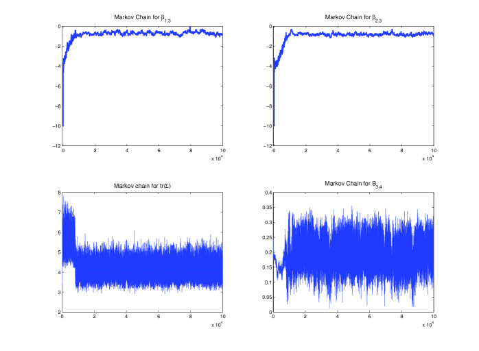
Figure 1: Sample paths for posterior parameters, using 100 data points, true rank of $r=2$ known and an adaptive MCMC algorithm.

These results demonstrate that both Algorithm 1 and Algorithm 2 perform well. The MMSE estimates produced by both algorithms are accurate compared to the true parameter values used to generate the data. Algorithm 1 which involved the mixture of pretuned local moves and a Global move centered on the Maximum Likelihood parameter estimates required more computational effort than the adaptive MCMC approach of Algorithm 2. Additionally, we point out that as discussed in Rosenthal (2008), the sampler we developed in Algorithm 2 actually achieves optimal performance as $n\rightarrow\infty$. Therefore it will be a far superior algorithm to the griddy Gibbs sampler approach which will not be feasible in high dimensions. Hence, for an automated and computationally efficient alternative to the griddy Gibbs sampler typically used we would recommend the use of Algorithm 2. In the following studies, we utilize Algorithm 2, the adaptive MCMC algorithm. To conclude, we also present the trace plots of the sample paths under the adaptive MCMC algorithm, see Figure 1. This plot demonstrates that rapid convergence of the MMSE estimates of the parameters in the posterior, even when initialized far from the true values. Additionally, one can see the behavior of the adaptive proposal, learning the appropriate proposal variance.

6.1.2 Analysis of Adaptive MCMC sampler in high dimension.

In this example, we work with the Adaptive MCMC algorithm we developed for the Bayesian CVAR model. In particular we consider the case in which $n=10$, which is a setting in which the standard approach of the griddy Gibbs sampler will become excessively computational, due to the curse of dimensionality, since there are now several hundred parameters to be sampled from the posterior.

All coefficients except for the cointegrating vectors are generated by uniform distributions with a range between -0.4 to 0.4, and the error covariance was set to the identity. We generate a realizations of data of length $T=100$ from the true rank $r=5$ model in which the cointegration vector has all terms in the matrix of $\bm{\beta}$ which are unrestricted set to be 0, other than the last row, which is -1. Then conditional on knowledge of the rank $r=5$ we sample $J=20,000$ samples from the joint posterior $p\left(B,\Sigma,\bm{\beta}|Y,r=5\right)$ and discard the first 10,000 samples as burnin.

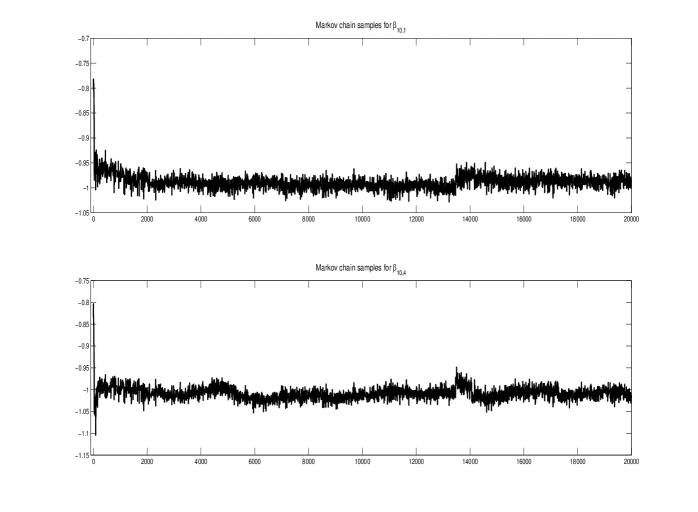
Figure 2: Sample paths for posterior parameters, using 100 data points, true rank of $r=5$ known and an adaptive MCMC algorithm.

The sample paths of the cointegration vector parameters randomly selected to be presented were $\beta_{10,1},\beta_{10,4}$ which are shown in Figure 2. Clearly, again in this high dimensional setting (310 dimensions), the adaptive MCMC algorithm performs suitably. Even, though the Markov chain is initialized far from the true parameter values of cointegration vector, we see the rapid convergence of our sampler. This is illustrated for the two arbitrarily selected parameters which had true values of of -1 and -1. Note, in this high dimensional setting, the algorithm was implemented in Matlab and took only 132sec to complete the simulation on an Intel Core 2 Duo at 2.40GHz, with 3.56Gb of RAM.

6.1.3 Analysis of model selection in the Bayesian CVAR model

In this section we study on synthetic data the performance of the Bayes Factor estimator applied to estimate posterior model probabilities for the rank. To perform this analysis we consider the model from Sugita, (2002; 2009 [p.4]) and we take data series of length $T=100$ and we simulate 50 independent data realizations for each possible model rank $r=1,\ldots,4$. Then for each rank $r$ we count the number of times each model is selected as the MAP estimate out of the total of the 50 simulations, one simulation per generated data set. Note, the algorithm was run for 20,000 iterations with 10,000 samples used as burnin. The results of this analysis are presented in Table 2.

We note that the results of this section demonstrated the following interesting properties:

1. When the true rank used to generate the observations data was small, the BF methodology was clearly able to detect the true model order as the MAP estimate in a high proportion of the tested data sets.

2. In all cases the averaged actual posterior model probabilities were very selective of the correct model, indicating that at least under this synthetic data scenario, there would not be great benefit in performing model averaging. However, we will demonstrate later examples with actual data in which there is significant ambiguity between possible model ranks, in these cases we also study the model averaging results.

6.2 Financial Example 1 - US mini indexes

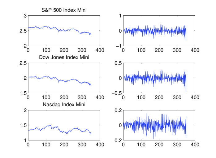
Figure 3: S&P 500, Dow Jones and Nasdaq mini Index daily close price data between 01-May-08 to 18-Sep-08. Left column plots represent scaled raw prices; Right plots represent difference data series.

Having assessed the proposed algorithms developed in this paper for synthetic data generated from a CVAR model, we now work with a practical financial example. In this example we will consider data series comprised of US indexes S&P mini, Nasdaq mini and Dow Jones mini. The data obtained for each of these data series consists of 774 values corresponding to the close of market daily price from the 31-Aug-2005 through to 30-Sep-2008. The time series data is presented in Figure 3.

We analyze this data using Algorithm 2 (adaptive MCMC) and estimate the rank via Bayes Factor analysis, the results are presented in Table 3. We run 20 independent samplers with different initializations, for each possible rank. This is performed for each data set, and the total series is split into increasing subsets, each taking subsets of the data from 50 data points through to 400 data points, in increases of 50 data points. This allows us to study the change in the estimated rank as a function of time for each of these time series. Clearly, if the true rank of our model was fixed, then as the total amount of data we include increases, then we should see the posterior model probability of the rank converge to 1 for one of the possible ranks. What we observed after doing this analysis was that there was a clear variability in the predicted rank as we included more data. In particular the model estimates showed preference most often to rank 1, suggesting that 2 common stochastic trends are present in the series. Additionally, the fact that in several cases, the model is less likely to distinguish between rank 1 and 2, suggests it may be prudent to also perform a model averaging analysis. Especially in the popular application of CVAR models in practice to perform algorithmic trading.

6.3 Financial Example 2 - US notes

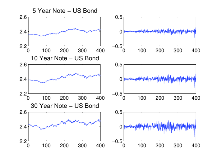
Figure 4: 5, 10, 30 Year Notes - daily close price data between 01-May-08 to 18-Sep-08. Left column plots represent scaled raw prices; Right plots represent difference data series.

Here we repeat the same procedure performed in Financial Example 1, for a different data set. This time we consider data series comprised of Bond data for US 5 year, 10 year and 30 year notes over the same time period as the US mini index data. The time series data is presented in Figure 4.

We analyze this data using Algorithm 2 (adaptive MCMC) and estimate the rank via Bayes Factor analysis, the results are presented in Table 4. We set up this second data analysis in the same way as Financial Exampl 1, with 20 independent samplers, each with different initializations, for each possible rank. This allows us to study the change in the estimated rank as a function of time for each of these time series. Again, we observed that with this data, the model gave preference most often to rank 1, suggesting that 2 common trends are present in the series we are analyzing. However, there was much stronger evidence for a single co-integrating relationship over time in this data, compared to the analysis of the US mini index data over the same period. This suggests that the US bond data series is a more stable series to fit the CVAR model too when assuming a constant number of co-integrating relationships over time.

6.4 Financial Example 3

In this section we perform a predictive performance comparison using Bayesian Model Selection versus Averaging. We take 2 series for the US bonds, 5 years and 10 years, and we combine these series over the same period with the S& P 500 mini index. We compare the MMSE estimate of the predicted series over 10 steps ahead which is obtained from the distribution of the predicted data $p\left(Y^{*}|Y\right)$, after we have integrated out parameter and rank uncertainties. We demonstrate that in this actual data example, the performance obtained by Bayesian Model Averaging represents the uncertainty in the prediction more accurately than the Bayesian Model Order Selection setting.

This study is performed as follows. We begin by selecting randomly, with replacement, 100 segments of the vector time series, each containing 50 days of data. For each segment of the time series we fit our Bayesian model for each possible rank, also estimating via Bayes Factors the posterior model probability for each rank. Then we calculate the predictive posterior mean, corresponding to the MMSE estimate of the predicted data series for the following 5 days, $Y^{*}$. Finally, we take the squared difference between the actual data series over the proceeding 10 days post the 50 days for the given segment and the posterior mean of the predicted data $Y^{*}$.

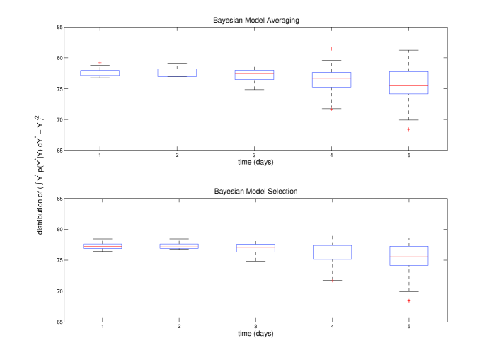
Figure 5: Empirical distribution of the Bayesian Model Averaging and Bayesian Model Order Selection, predictive performance for a combination of mini-index and bond data, taken over random intervals.

In Figure 5 we present for each prediction day a boxplot of the squared difference between the actual data over the random sets of 5 days and the predictive posterior MMSE estimators for the same 5 days. We compare here the performance under Bayesian model selection and averaging. When performing Bayesian model averaging we are integrating out uncertainty in the prediction due to the prediction of the unknown rank.

Clearly, the Bayesian model averaging approach will result in a greater uncertainty in the prediction when compared to the Bayesian model selection. This is reflected especially in the distribution of the prediction at 5 days where the model averaging approach box-whisker plot covers a noticeably wider range than the model selection equivalent. Though not presented here, we also assessed and confirmed this would occur out to longer predictions of 10 days and 20 days.

7 Conclusions

We have developed and demonstrated how one can utilize state of the art adaptive MCMC methodology to solve a challenging high dimensional econometrics problem based on cointegrated vector autoregressions. The challenging application involved a posterior distribution which was matrix-variate and very high dimensional. We compared the performance of the Adaptive Metropolis algorithm with an alternative based on a mixture proposal of local and global moves centered on the the Maximum Likelihood parameters. We then formulated the rank estimation in as a Bayesian model selection problem and performed analysis of the Bayes factors using our adaptive MCMC algorithm. We concluded with analysis of real market data and performed Bayesian model selection and model averaging, with respect to the unknown rank. In conclusion, the adaptive MCMC methodology developed clearly allowed us to extend significantly the dimension of the estimation problem in the Bayesian CVAR literature. It was shown to be highly efficient and accurate.

From the perspective of developing a Bayesian CVAR model for algorithmic trading we found that historically the US bond data we considered is a more stable series to fit the CVAR model too when assuming a constant number of co-integrating relationships over time. This will therefore impact the stability of trading performance under such models. In addition when considering trading triples made up of the US bond data series and the S&P mini index, it is beneficial to perform Bayesian model averaging for the rank, rather than just selecting the most probable co-integration rank. The adaptive MCMC based framework allows this to be done efficiently and in an automated fashion.

8 Acknowledgments

We would like to thank Prof. Robert Kohn for useful feedback and also we thank the two anonymous referees and associate editor for their very helpful comments which have significantly improved the exposition of the paper. The first author thanks the Statistics Department of the University of NSW for financial support and Boronia Managed Funds.

9 References

1. Andrieu, C., Moulines, E. (2006). ”On the ergodicity properties of some adaptive MCMC algorithms”. Annals of Applied Probability, 16, (3).

2. Andrieu, C., Atachade, Y. (2007). ”On the efficiency of adaptive MCMC algorithms”. Electronic Communications in Probability, 12, 336-349.

3. Atachade, Y.F., Rosenthal, J.S. (2005). ”On adaptive Markov chain Monte Carlo algorithms”. Bernoulli, 11(5), 815-828.

4. Bauwens, L., Lubrano, M. (1996). ”Identification restrictions and posterior densities in cointegrated Gaussian VAR systems”. Advances in Econometrics 11, Part B, (JAI Press, Greenwich) 3-28.

5. Bauwens, L., Giot, P. (1997). ”A Gibbs sampling approach to cointegration”. Computational Statistics, 13, 339-368.

6. Chib, S, (1995). ”Marginal likelihood from the Gibbs output”. Journal of the American Statistical Association, 90(432), Theory and Methods, 1313-1321.

7. Engle, R.F., Granger, C.W.J. (1987). ”Co-Integration and Error Correction: Representation, Estimation, and Testing”. Econometrica, 55(2), 251-276.

8. Fan, Y., Peters, G.W., Sisson, S.A. (2009). ”Automating and evaluating reversible jump MCMC proposal distributions”. Statistics and Computing, 19, 409-421.

9. Geweke J. (1996). ”Bayesian reduced rank regression in econometrics”. Journal of Econometrics, 75, 121-146.

10. Giordani, P. and Kohn, R. (2006). ”Adaptive independent Metropolis-Hastings by fast estimation of mixtures of normals.” Preprint.

11. Granger, C.W.J. (1981). ”Some properties of time series data and their use in econometric model specification”. Journal of Econometrics, 121-130.

12. Granger, C.W.J., Weiss, A.A. (1983). ”Time series analysis of error-correcting models”. Studies in econometrics, time series, and multivariate statistics. New York: Academic Press, 255-278.

13. Haario, H., Saksman, E., Tamminen, J. (2007). ”Componentwise adaptation for high dimensional MCMC”. Computational Statistics, 20(2).

14. Haario, H., Saksman, E., Tamminen, J. (2001). ”An adaptive metropolis algorithm”. Bernoulli, 7, 223-242.

15. Kleibergen, F., Paap, R. (2002). ”Priors, posteriors and Bayes factors for a Bayesian analysis of cointegration”. Journal of Econometrics, Elsevier, 111(2), 223-249.

16. Kleibergen, F., van Dijk, H.K. (1994). ”On the Shape of the Likelihood/Posterior in Cointegration Models”. Econometric Theory, Cambridge University Press, 10(3-4), 514-551.

17. Koop, G., Strachan, R., van Dijk, H., Villani, M. (2006). ”Bayesian Approaches to Cointegration”. In T.C.Mills and K. Patterson (Ed.), Palgrave Handbook of Econometrics Volume 1 Econometric Theory 1st ed. (pp. 871-898) UK: Palgrave Macmillan.

18. Lütkepohl, H. (2007). New Introduction to Multiple Time Series Analysis. Springer

19. Peters, G.W., Kannan, B.K., Lasscock, B., Mellen, C. (2009). ”Trans-dimensional and adaptive Markov chain Monte Carlo for Bayesian co-integrated VAR models”. Technical Report: University of NSW, Statistics Department.

20. Reinsel, G.C., Velu, R.P. (1998). Multivariate Reduced-Rank Regression, Theory and Applications. Lectuer Notes in Statistics Springer.

21. Roberts, G.O., Gelman, A., Gilks, W.R. (1997). ”Weak convergence and optimal scaling of random walk Metropolis algorithms”. Annals of Applied Probability, 7, 110-120.

22. Roberts, G.O., Rosenthal, J.S. (2009). ”Examples of Adaptive MCMC”. Journal of Computational and Graphical Statistics, 18(2), p.349-367.

23. Roberts, G.O., Rosenthal, J.S. (2001). ”Optimal scaling for various Metropolis-Hastings algorithms”. Statistical Science, 16, 351-367.

24. Rosenthal, J.S. (2008). ”Optimal Proposal Distributions and Adaptive MCMC”. Chapter for MCMC Handbook, Brooks S., Gelman A., Jones G. and Meng X.L. eds.

25. Silva, R., Giordani, P., Kohn, R., Pitt, M. (2009). ”Particle filtering within adaptive Metropolis Hastings sampling.” Arxiv preprint arXiv:0911.0230.

26. Strachan, R.W., van Dijk, H.K. (2004). ”Bayesian model selection with an uninformative prior”. Keele Economics Research Papers

27. Strachan, R.W., van Dijk, H.K. (2007). ”Bayesian model averaging in Vector Autoregressive Processes with an Investigation of Stability of the US Great Ratios and Risk of a Liquidity Trap in the USA, UK and Japan”.

28. Strachan, R.W., Inder, B. (2004). ”Bayesian analysis of the error correction model”. Journal of Econometrics, 123(2), 307-325.

29. Sugita, K. (2002). ”Testing for cointegration rank using Bayes factors”. Royal Economic Society Annual Conference, Royal Economic Society.

30. Sugita, K. (2009). ”A Monte Carlo comparison of Bayesian testing for cointegration rank”. Economics Bulletin, 29(3), 2145-2151.

31. Verdinelli, I. and Wasserman, L. (1995). ”Computing Bayes Factors Using a Generalization of the Savage-Dickey Density Ratio”. Journal of the American Statistical Association, 90(433).

32. Vermaak,J., Andrieu, C., Doucet, A., Godsill, S.J. (2004). ”Reversible jump Markov chain Monte Carlo strategies for Bayesian model selection in autoregressive processes”. Journal of Time Series Analysis, 25(6), 785-809.

10 Appendix 1

We begin by calculating the log posterior model probabilities,

$$\text{log}\left(Pr\left(r|Y\right)\right)=\text{log}\left(BF_{r|0}\right)+\text{log}\left(BF_{max|0}\right)-\text{log}\left(\sum^{n}_{j=0}\text{exp}\left(\text{log}\left(BF_{j|0}\right)-\text{log}\left(BF_{max|0}\right)\right)\right),$$ (10.1)

where $BF_{max|0}=max\{BF_{0|0},...,BF_{n|0}\}$. Additionally, we now consider the log of the Bayes Factor for rank $r$ and we apply the same numerical trick.

$$\text{log}\left(BF_{r|0}\right)=\text{log}\left(p(\bm{\alpha}^{\prime}=0_{r\times n})\right)+\text{log}\left(C_{r}\right)-\text{log}\left(p(\bm{\alpha}^{\prime}=0_{r\times n}|Y)\right)$$ (10.2)

Now, considering each of the terms:

• $\text{log}\left(p(\bm{\alpha}^{\prime}=0_{r\times n})\right)=-\frac{nr}{2}\text{log}(\pi)+\frac{h}{2}\text{log}\left(|S|\right)+\frac{n}{2}\text{log}\left(|A_{22.1}|\right)+\sum_{j=1}^{n}\text{log}\left(\frac{\Gamma(\frac{h+r+1-j}{2})}{\Gamma(\frac{h+1-j}{2})}\right)-\frac{h+r}{2}\text{log}\left(|S|\right)$

• $\text{log}\left(p(\bm{\alpha}^{\prime}=0_{r\times n}|Y)\right)=-\text{log}\left(N\right)+\text{log}\left(L^{(1)}_{max}\right)-\text{log}\left(\text{exp}\left(\sum^{N}_{i=1}\text{log}\left(L^{(1)}_{i}\right)-\text{log}\left(L^{(1)}_{max}\right)\right)\right)$,
  where $L^{(1)}_{i}=\pi^{-\frac{nr}{2}}|S_{*}^{(i)}|^{\frac{t+h}{2}}|A_{*22,1}^{(i)}|^{\frac{n}{2}}{\prod_{i=1}^{n}\frac{\Gamma(\frac{t+h+r+1-i}{2})}{\Gamma(\frac{t+h+1-i}{2})}}|S_{*}^{(i)}+B_{*2}^{(i)^{\prime}}A_{*22.1}^{(i)}B_{*2}^{(i)}|^{-\frac{t+r}{2}}$ and $L^{(1)}_{max}=\text{max}\{L^{(1)}_{1},...,L^{(1)}_{N}\}$.

• $\text{log}\left(C_{r}\right)=-\text{log}(N)+\text{log}\left(L^{(2)}_{max}\right)\text{log}\left(\text{exp}\left(\sum^{N}_{i=1}\text{log}\left(L^{(2)}_{i}\right)-\text{log}\left(L^{(2)}_{max}\right)\right)\right)$,
  where $L^{(2)}_{i}=\frac{p(\bm{\alpha}=0,\Gamma^{(i)}|\Sigma^{(i)})}{p(\Gamma^{(i)}|\Sigma^{(i)})}$ and $L^{(2)}_{max}=\text{max}\{L^{(2)}_{1},...,L^{(2)}_{N}\}$. Note this sum evaluated using samples from the Markov chain run in model $r$ where, $p(\bm{\alpha}=0,\Gamma^{(i)}|\Sigma^{(i)})$ and $p(\Gamma^{(i)}|\Sigma^{(i)})$ are obtained using knowledge of the specified prior, $p(B|\Sigma)=p(\Gamma,\bm{\alpha}|\Sigma)=p(\mu,\Psi_{1:p-1},\bm{\alpha}|\Sigma)$.

Parameter Estimates	Algorithm 1	Algorithm 2	Truth
Ave. MMSE $\beta_{1,r+1}$	-0.002 (0.001)	-0.034 (0.002)	0
Ave. Posterior Stdev. $\beta_{1,r+1}$	0.018 (0.006)	0.010 (0.003)	-
Ave. MMSE $\beta_{2,r+1}$	-0.819 (0.051)	-0.862 (0.045)	-1
Ave. Posterior Stdev. $\beta_{2,r+1}$	0.032 (0.005)	0.020 (0.003)	-
Ave. MMSE $\beta_{1,n}$	0.033 (0.025)	-0.024 (0.023)	0
Ave. Posterior Stdev. $\beta_{1,n}$	0.030 (0.012)	0.026 (0.010)	-
Ave. MMSE $\beta_{2,n}$	-0.752 (0.098)	-0.774 (0.082)	-1
Ave. Posterior Stdev. $\beta_{2,n}$	0.038 (0.013)	0.028 (0.006)	-
Ave. Mean acceptance probability $\bm{\beta}$	0.352 (0.010)	0.232 (0.029)	-
Ave. MMSE $\text{tr}\left(\Sigma\right)$	4.945 (0.331)	4.432 (0.332)	4
Ave. Posterior Stdev. $\text{tr}\left(\Sigma\right)$	0.420 (0.049)	0.416 (0.048)	-
Ave. MMSE $\mu_{1}$	0.07 (0.051)	0.065 (0.043)	0.1
Ave. Posterior Stdev. $\mu_{1}$	0.236 (0.028)	0.226 (0.026)	-
Ave. MMSE $\mu_{2}$	-0.027 (0.041)	-0.034 (0.024)	0.1
Ave. Posterior Stdev. $\mu_{2}$	0.183 (0.041)	0.181 (0.010)	-
Ave. MMSE $\mu_{3}$	-0.080 (0.084)	-0.061 (0.045)	0.1
Ave. Posterior Stdev. $\mu_{3}$	0.199 (0.020)	0.187 (0.015)	-
Ave. MMSE $\mu_{4}$	0.024 (0.049)	0.030 (0.029)	0.1
Ave. Posterior Stdev. $\mu_{4}$	0.184 (0.010)	0.185 (0.011)	-
Ave. MMSE $\alpha_{1,1}$	-0.223 (0.015)	-0.224 (0.016)	-0.2
Ave. Posterior Stdev. $\alpha_{1,1}$	0.070 (0.006)	0.068 (0.005)	-
Ave. MMSE $\alpha_{1,2}$	0.201 (0.013)	0.202 (0.013)	0.2
Ave. Posterior Stdev. $\alpha_{1,2}$	0.053 (0.002)	0.052 (0.002)	-

Table 1: Sampler Analysis - Algorithm 1 is the pretuned mixture proposal of Global ML move and local pretuned MCMC move; Algorithm 2 is the Global adaptively learnt MCMC proposal. Averages and a standard error are taken for the Bayesian point estimators over 20 data sets, the standard errors are presented in brackets $(\cdot)$. Note in all simulations the initial Markov chain is started very far away from the true parameter values.

Model Rank	Bayes Factors
$r=0$	3 (0.84)
$\bf{r=1}$	16 (0.93)
$r=2$	2 (0.92)
$r=3$	0 (-)
$r=4$	0 (-)
$r=0$	0 (-)
$r=1$	5 (0.89)
$\bf{r=2}$	13 (0.91)
$r=3$	0 (-)
$r=4$	2 (0.92)
$r=0$	0 (-)
$r=1$	0 (-)
$r=2$	4 (0.89)
$\bf{r=3}$	6 (0.90)
$r=4$	10 (0.94)
$r=0$	0 (-)
$r=1$	0 (-)
$r=2$	0 (-)
$r=3$	2 (0.87)
$\bf{r=4}$	18 (0.89)

Table 2: Between Model Analysis - The true model rank used to generate the data is presented in bold. TDMCMC is the Trans-dimensional Markov chain Monte Carlo algorithm utilizing adaptive MH within model moves and the global Independent between model moves. The results represent the total number of times a given rank is selected as the MAP estimate out of the 20 independent data sets, each of length T=100, analyzed. Additionally, the average posterior model probability for these cases is presented in brackets.

Rank $\setminus$ T	50	100	150	200	250	300	350	400
$r=0$	0	0	0	0	0	0	0	0
$r=1$	8.09 (0.78)	3.77 (0.29)	7.01 (0.50)	11.51 (0.90)	1.69 (0.54)	2.71 (3.55)	3.14 (1.11)	7.77 (0.83)
$r=2$	2.91 (1.24)	2.33 (1.26)	4.61 (0.63)	25.36 (7.19)	-5.33 (1.17)	-5.80 (0.97)	4.92 (1.06)	-3.88 (1.11)
$r=3$	-26.03 (1.06)	-8.45 (0.27)	-37.25 (1.08)	-55.79 (1.70)	-14.61 (0.03)	-62.60 (3.31)	$8.88$ ($0.88$) $\times 10^{-3}$	-2.06 ($2.48\times 10^{-2}$)

Table 3: Log Bayes Factors: Analysis of VAR series of US mini indexes as a function of data size. Average log Bayes Factors and standard deviation of log Bayes Factors over 20 independent Markov chains each of chain length 20,000.

Rank $\setminus$ T	50	100	150	200	250	300	350	400
$r=0$	0	0	0	0	0	0	0	0
$r=1$	4.81 (1.00)	3.14 (0.43)	5.36 (1.06)	5.92 (0.84)	3.32 (0.75)	1.30 (0.37)	7.30 (0.59)	3.10 (0.48)
$r=2$	-1.67 (12.78)	3.66 (3.87)	-3.75 (3.04)	-1.83 (2.61)	-6.02 (3.22)	0.14 (6.51)	-2.93 (1.96)	-7.73 (2.46)
$r=3$	-42.44 (12.38)	-48.58 (2.85)	-33.12 (0.14)	-100.42 (4.82)	$-25.91(6.52\times 10^{-2})$	-10.33 (0.72)	-142.89 (3.31)	-195.47 (4.71)

Table 4: Log Bayes Factors: Analysis of VAR series of US Bonds (5,10,30 Year Notes) as a function of data size. Average log Bayes Factors and standard deviation over 20 independent Markov chains each of chain length 20,000.