Table 1. Sub-My Asteroid Clusters

Table 2. Asteroid Pair Photometry

Table 3. S-complex sub-My cluster members’s derived spectral and age data

Table 4. Asteroid Pairs

47 pages

7 figures

4 tables

Running Head: Space weathering and gardening rates on S-complex asteroids

Editorial correspondence to:

Mark Willman

Institute for Astronomy University of Hawaii’i at Manoa

2680 Woodlawn Drive, Honolulu, HI 96822

willman@ifa.hawaii.edu

808-956-6989 tel

808-956-9580 fax

We have extended our earlier work on space weathering of the youngest S-complex asteroid families to include results from asteroid clusters with ages $<10^{6}$ years and to newly identified asteroid pairs with ages $<5\times 10^{5}$ years. We have identified three S-complex asteroid clusters amongst the set of clusters with ages in the range $10^{5-6}$ years — (1270) Datura, (21509) Lucascavin and (16598) 1992 YC2. The average color of the objects in these clusters agrees with the color predicted by the space weathering model of Willman et al. , (2008). SDSS 5-filter photometry of the members of the very young asteroid pairs with ages $<10^{5}$ years was used to determine their taxonomic classification. Their types are consistent with the background population near each object. The average color of the S-complex pairs is $PC_{1}=0.49\pm 0.03$, over 5$\sigma$ redder than predicted by Willman et al. , (2008). This may indicate that the most likely pair formation mechanism is a gentle separation due to YORP spin-up leaving much of the aged and reddened surface undisturbed. If this is the case then our color measurement allows us to set an upper limit of $\sim 64\%$ on the amount of surface disturbed in the separation process. Using pre-existing color data and our new results for the youngest S-complex asteroid clusters we have extended our space weather model to explicitly include the effects of regolith gardening and fit separate weathering and gardening characteristic timescales of $\tau_{w}=960\pm 160$ My and $\tau_{g}=2000\pm 290$ My respectively. The first principal component color for fresh S-complex material is $PC_{1}=0.37\pm 0.01$ while the maximum amount of local reddening is $\Delta PC_{1}=0.33\pm 0.06$. Our first-ever determination of the gardening time is in stark contrast to our calculated gardening time of $\tau_{g}\sim 270$ My based on main belt impact rates and reasonable assumptions about crater and ejecta blanket sizes. A possible resolution for the discrepancy is through a ‘honeycomb’ mechanism in which the surface regolith structure absorbs small impactors without producing significant ejecta. This mechanism could also account for the paucity of small craters on (433) Eros.

Keywords: Asteroids, surfaces; Spectrophotometry; Spectroscopy

1 Introduction

After three decades of development our understanding of the space weathering phenomenon may be converging on its cause and effects. Originally proposed (Chapman and Salisbury,, 1973) as a solution to the mismatch between the color of the most common meteorites, ordinary chondrites, and their likely source region, inner main belt S-complex asteroids, the space weathering hypothesis is that the surface colors of asteroids change with exposure to the space environment (Hapke,, 1973, 1968). The idea has held up to the test of time and in recent years has led to measurements of the rate of color change on S-complex asteroids yielding empirical models that predict the rate of reddening of their surfaces (Jedicke et al. ,, 2004; Nesvorný et al. ,, 2005; Willman et al. ,, 2008). This work extends our space weathering model to the youngest dated asteroids in the main belt that are less than $10^{6}$ years old and, for the first time, measures the surface gardening rate on the asteroids due to impact-generated regolith cycling.

Willman et al. , (2008)’s space weathering model applies exclusively to S-complex asteroids. Other types of asteroids may also undergo space weathering and we expect that they would obey a model of similar functional form with different parameters. For instance, if C-complex asteroids undergo space weathering they must have a different color range because they occupy a different region of principal component space and the weathering rate and even the sense of coloration may be different (Nesvorný et al. ,, 2005). The gardening rate would probably also be different due to different material density and strength.

In this work we study the space weathering of S-complex asteroids without particular concern for the agent causing the weathering though the likely culprit is energy deposition due to particle bombardment e.g. micrometeorites, solar protons and cosmic rays. Marchi et al. , (2006) claim that Sun-related effects are dominant but they assumed that micrometeorite impacts are independent of heliocentric distance. Since neither their flux nor their velocity are distance independent (Cinatala,, 1992) it is unclear whether it is justified to downgrade their contribution to the space weathering agent inventory. Laboratory-based studies suggest that the asteroidal space weathering mechanism, long confused with the lunar processes producing agglutinates, involves the coating of near surface semi-transparent nanophase grains by a vapor or sputter deposited film of metallic iron (e.g.  Sasaki et al. ,, 2001; Pieters et al. ,, 2000).

While measuring the color of asteroid surfaces is relatively straightforward and asteroid taxonomy based on colors has been a mainstay of planetary science for decades the determination of asteroid surface ages is a relatively recent innovation. The surface ages of asteroid family members may be determined from dynamical simulations of the evolution of the family’s orbit element distribution(e.g.  Vokrouhlický and Nesvorný, 2006a, ; Vokrouhlický et al. ., 2006b, ; Nesvorný et al. ,, 2005, 2002; Marzari et al. ,, 1995). The dynamical methods include family size frequency distribution (SFD) modeling, global main belt SFD modeling, modeling of family spreading via thermal forces and backward numerical integration of orbits. The combination of asteroid surface colors with their ages allowed the first astronomical determination of the space weathering rate (Jedicke et al. ,, 2004; Parker et al. ,, 2008).

Space weathering rate measurements utilize the fact that asteroid family members are fragments of a single collisionally disrupted parent body that formed at the same time and assume that fresh unweathered material from the collision debris cloud coats all members of a family with a homogeneous regolith layer. Therefore, all family members should start out with similar color and weather in tandem.

We ignore grain size color effects for a number of reasons. First, we believe that unless grain size is correlated with age its effect will average out over the members of a family. Second, we will see below that km scale asteroids, in contrast to moon sized bodies with highly comminuted regoliths, are gravitationally sorted rubble piles whose surfaces are dominated by boulders. Fines are largely absent, perhaps sequestered beneath the bouldered surface, so asteroid regolith appears to vary with size. This would diminish grain size observational effects in the sub-milligee environment of small asteroids. Finally, Nesvorný et al. , (2005) and Jedicke et al. , (2004) did not find any correlation between color and size, just color and age.

Jedicke et al. , (2004)’s space weathering rate measurements encapsulated ‘the color’ of an asteroid’s surface as its first principal component color

$$PC_{1}=0.396\;(u-g)+0.553\;(g-r)+0.567\;(g-i)+0.465\;(g-z)$$ (1)

that correlates strongly with the average slope of the spectrum. The principal component color provides the linear combination of filter magnitudes having the greatest variability over the sample of asteroids. In this case $PC_{1}$ is specific to the asteroids in the Sloan Digital Sky Survey (SDSS) 2^nd Moving Object Catalog. While most of the color variability in the SDSS asteroid sample is captured in $PC_{1}$, the second principal component,

$$PC_{2}=-0.819\;(u-g)+0.017\;(g-r)+0.090\;(g-i)+0.567\;(g-z),$$ (2)

(Nesvorný et al. ,, 2005) corresponds to the asteroid spectrum’s curvature and is used in this analysis to identify asteroid taxonomy.

Motivated by the fact that uniform surface irradiation should produce an exponentially decaying amount of unweathered surface Jedicke et al. , (2004) showed that the color of S-complex asteroids as a function of time $t$ can be expressed as

$$PC_{1}(t)=PC_{1}(0)+\Delta PC_{1}[1-e^{-(t/\tau)^{\alpha}}]$$ (3)

where $PC_{1}(0)$ is the unweathered color of fresh surface material, $\Delta PC_{1}$ is the magnitude of the weathering color change after a long period of time, $\tau$ is the characteristic time for space weathering and $\alpha$ is a generalizing exponent. Willman et al. , (2008) improved upon the earlier work by refining the color of the $\lower 2.0pt\hbox{$\,\buildrel\scriptstyle<\over{\scriptstyle\sim}\,$}5$ My old Iannini family, eliminating the Eos family that is no longer considered to be in the S-complex, and carefully refitting the data to the functional form given above to determine $PC_{1}(0)=0.31\pm 0.04$, $\Delta PC_{1}=0.31\pm 0.07$, $\tau=570\pm 220$ My and $\alpha=0.53\pm 0.19$.

The characteristic time scale of $570\pm 220$ My for color change in the main asteroid belt (Willman et al. ,, 2008) is in agreement with pulsed laser experiments (Sasaki et al. ,, 2001) on silicate pellets intended to simulate micrometeorite bombardment. They suggested a characteristic time for weathering of 100 My at $1$ AU, equivalent to about 700 My in the main belt assuming that the Sun is the source of the weathering agent and a $r^{-2}$ dependence on its strength. However, (Loeffler et al. ,, 2009) argue that Sasaki et al. , (2001) overestimated the space weathering characteristic timescale due to an incorrect flux calculation leading. Basically, the time scale extrapolation from lab results is complicated because it is unclear how to evaluate the contribution from several different factors. For instance, in the main belt micrometeorite impact speeds will be lower ($\sim 5$ km/s) than at 1 AU ($\sim 20$ km/sec) and their impact energy will be $\sim$16x weaker.

Pieters et al. , (2000) estimated characteristic aging times of $100-800$ My for lunar surfaces by comparing ages from craters dated radiometrically or by cosmic ray exposure ages to spectral differences. Correcting the rate to the center of the main belt suggests weathering times on the order of $\sim$600-4800 My. Even though the lunar surface is not identical to S-complex asteroid surfaces the time scales are similar.

Finally, we note that craters on (243) Ida are bluer than their surrounding background terrain (Veverka et al. ,, 1996). The craters correspond to freshly exposed and unweathered regolith (Veverka et al. ,, 1996) while other parts of the asteroid’s surface indicates an age of about 1 Gy (Greenberg et al. ,, 1996). The wide range in diameters (a proxy for crater age) of blueish crater suggests that the space weathering time must be long.

On the other hand there are claims of faster surface weathering time scales such as Takato, (2008)’s upper limit of 450 kyr based on a shallow 1 $\mu$m absorption band observed on (1270) Datura. However, we expect that the space weathering phenomenon is a relatively subtle effect easily masked by stochastic variations between asteroids due to i.e. mineralogical and morphological differences and/or collisional and cratering events. The space weathering effect can only be identified in specific regions on an asteroid as observed with in situ spacecraft measurements on (951) Gaspra (Helfenstein et al. ,, 1994), (243) Ida (Veverka et al. ,, 1996), and (25143) Itokawa (Ishiguro et al. ,, 2007)] or as an ensemble effect on a statistically large sample of asteroids. It is therefore difficult to make a general conclusion based on a single asteroid such as (1270) Datura. Indeed, our measurement of that asteroid’s $PC_{1}=0.41\pm 0.02$ is redder by $2.2\sigma$ than its predicted color from Willman et al. , (2008). Takato’s measurement of a shallow 1 $\mu$m absorption band which would tend to redden the overall spectrum is therefore generally consistent with our measurement. We expect that the ‘redness’ of individual small rubble pile asteroids in a sample is affected more by random surface variations than larger regolith-rich asteroids with finer surface materials. In this case (1270) Datura is redder than the Datura cluster average so its particular value can be misleading. The four (1270) Datura members in this work have mean $PC_{1}=0.305$ with a RMS of $0.278$. The large standard deviation is not due to measurement error — it is a result of intrinsic color differences between the members of the (1270) Datura family and is typical of other families. Therefore we would discount the resulting 450 kyr weathering time.

Another short time scale measurement was reported from recent lab experiments on olivine powder by Loeffler et al. , (2009) (and references therein) simulating solar wind effects at 1 AU by bombardment with 4 keV protons. They conclude that spectral reddening caused by the solar wind should saturate in $\sim$ 5 kyr.

(Vernazza et al. ,, 2009) combined spectral data from a sample of four members of young clusters with archival meteorite spectra and found that space weathering is substantially complete in $<$ 1 My but then continues at a slower pace up to several Gy. They attribute the first stage to the solar wind (Strazzulla et al. , (2008) lab simulation) and the second to micrometeorite bombardment. This scenario depends critically on the starting color that they derive from meteorite data.

It is not clear how to reconcile the information from these various lab results that differ in time scale by several orders of magnitude with our observations.

Willman et al. , (2008)’s weathering model was derived from families that were several My (e.g. Karin, Iannini) to several Gy (e.g. Eunomia, Maria) old. The family age estimates have typical errors of $\sim 40$% resulting from fundamental limitations in the dating techniques (Nesvorný et al. ,, 2007).

Although there were nine known S-complex families with ages from tens of Mys to a few Gys at that time there were only two younger than 10 My. Refining the space weathering rate at even younger ages requires a large sample of young asteroid families, which are typically produced by the catastrophic disruption of small asteroids, have only a small number of detectable members, and are therefore difficult to identify. But in recent years the number of catalogued asteroid orbits has reached hundreds of thousands and includes many asteroids smaller than 1 km. This large sample of asteroids allows the identification of rare small clusters originating from collisions less than 1 My ago. Nesvorný et al. , (2006); Nesvorný and Vokrouhlický, (2006) found four such clusters with a total of 16 members. The clusters are named after their largest known members: (1270) Datura, (14627) Emilkowalski, (21509) Lucascavin and (16598) 1992 YC2.

The progression to ever smaller clusters reached its logical limit with Vokrouhlický and Nesvorný, (2008)’s discovery of 60 pairs of asteroids in extremely similar orbits — much more alike than would be expected based on the density of proper elements for other asteroids with similar orbit elements. The pairs are thought to have formed less than 500 kyr ago based on the dynamical evolution time of the pair member’s orbits. Their list was updated and restricted to only 36 pairs (Pravec et al. ,, 2009). Pairs belonging to known young families such as (1270) Datura or (832) Karin were excluded because of the possibility that the catastrophic impact and subsequent family formation process may create paired asteroids. Such cases were eliminated to focus on pairs that were created in isolation and presumably by the same method. The formation method of pairs may involve a critical distinction from that of clusters or families. Whereas the latter form in catastrophic collisions, pairs have alternative possible formation methods. Some of these methods may be gentle processes not involving resetting of the surface as discussed in §6.3.

Shortly after the publication of Willman et al. , (2008) we obtained observations of some members of the sub-My old families and found that they were significantly redder than predicted. Did this imply a problem with our space weathering model or is the space weathering phenomenon more complicated than suggested by the simple model of eq. 3?

We were also concerned with the functional form of the space weathering model of Willman et al. , (2008) i.e. eq. 3. If space weathering is an isolated process the exponent $\alpha$ should be unity but Jedicke et al. , (2004) fit $\alpha=0.53\pm 0.19$. Their argument was that $\alpha$ is a generalizing factor that accounts for both space weathering and regolith gardening which acts to counteract the surface aging by slowing turning over the asteroid’s surface.

To investigate these questions we collected color and spectral data from several sources for members of the young families and pairs. We obtained spectra of members of the sub-My asteroid clusters (Nesvorný et al. ,, 2006; Nesvorný and Vokrouhlický,, 2006) and were provided spectra for some of the objects observed by Mothé-Diniz and Nesvorný, (2008). We also located archived photometry for 19 pair members in the Sloan Digital Sky Survey Data Release 7 Moving Object Catalog 4 (SDSS DR7 MOC4) (Parker et al. ,, 2008). We then developed a new asteroid surface color-age model that explicitly separates the effects of weathering and gardening and eliminates the need for the unexplained generalizing factor ($\alpha$). The new model allowed us to measure the characteristic timescales for both weathering and gardening on the S-complex asteroids. Finally, we independently calculated the gardening timescale on main belt asteroids from their size distribution, impact rates and estimates of crater and ejecta blanket size.

2 Space weathering versus regolith gardening effects

The space weathering model of Jedicke et al. , (2004) summarized in eq. 3 uses a characteristic time, $\tau$, along with a generalizing and unphysical exponent, $\alpha$, to capture the time dependence of the gradual reddening of S-complex asteroid surfaces. The exponent was introduced because it was understood that there are more effects in play on an asteroid’s surface than a single weathering component. e.g. multiple sources of space weathering with different time scales such as solar protons and ultraviolet radiation, micrometeorite bombardment and cosmic rays, in addition to the effect of regolith gardening which will counteract the space weathering. ‘Gardening’ is in part due to meteoroids that regularly strike the asteroids’s surface and lift fresh sub-surface material to the regolith’s top layer. Gardening may also take place through seismic shaking with subsequent regolith distribution or it may result from larger asteroid strikes which spread ejecta blankets beyond a crater. We do not distinguish between possible causes but lump them all under the banner of ’gardening’ in the same way that all possible causes of color change in minerals are included in ’weathering’. Here we extend the space weathering model of Jedicke et al. , (2004) to explicitly include both weathering and gardening.

Consider the relationship of unweathered surface, $U$, and weathered surface, $W$ — by construction $U+W=1$. Space weathering causes $U$ to be replaced by $W$ at the rate

$$\frac{dU^{-}}{dt}=-\frac{U(t)}{\tau_{w}}$$ (4)

where $\tau_{w}$ is the characteristic space weathering time. Regolith gardening causes $U$ to increase at the same rate that $W$ decreases,

$$\frac{dU^{+}}{dt}\equiv-\frac{dW}{dt}=\frac{W(t)}{\tau_{g}}$$ (5)

where $\tau_{g}$ is the characteristic gardening time.

The total rate of change of unweathered surface is then

$$\frac{dU}{dt}=\frac{dU^{+}}{dt}+\frac{dU^{-}}{dt}=\frac{1}{\tau_{g}}-\left(\frac{1}{\tau_{g}}+\frac{1}{\tau_{w}}\right)U.$$ (6)

Since $U(0)=1$

$$U(\tau_{g},\tau_{w},t)=\frac{e^{-\left(\frac{1}{\tau_{g}}+\frac{1}{\tau_{w}}\right)t}+\frac{\tau_{w}}{\tau_{g}}}{1+\frac{\tau_{w}}{\tau_{g}}}$$ (7)

which has the desired properties that $U(t=0)=1$ and as $t\rightarrow\infty$, $U\rightarrow(1+\frac{\tau_{g}}{\tau_{w}})^{-1}$ — the amount of unweathered asteroid surface after a long period of time is related to the relative rates of space weathering and regolith gardening.

Replacing the unweathered surface term in eq. 3 with our new generalized unweathered surface term in eq. 7 yields

$$PC_{1}(t)=PC_{1}(0)+\Delta PC_{1}[1-U(\tau_{w},\tau_{g},t)]$$ (8)

which includes the effects of both weathering and gardening and will allow the two characteristic times to be separately determined by fitting to the asteroid families’ color and age data.

Previous attempts to explore the relationship between weathered and unweathered surface have foundered on the fundamental equations. For instance, Gault et al. , (1974) overlooked the restorative effects of regolith gardening and assumed that the fraction of surface that is undisturbed is simply a decaying exponential in time.

We return to the model parameters that best fit the color-age data in §6.3. That gardening time determined from age-color data is compared to the resurfacing time determined from impacts in §6.4. In the next section we calculate the resurfacing rate using the independent method of impactors.

3 Calculating the resurfacing rate from impacts

The asteroid resurfacing rate due to impacts, $\dot{S}$, is the product of the frequency of impacts, $\nu(D)$, and the ejecta covered surface area, $A_{e}(D)$ per impact, where both terms are a function of impactor diameter $D$. Initially we place no limit on diameter which could extend from micrometeoroids up to parent body shattering size. The constraint on size will enter the discussion below in the lower limit of the impact integral. We realize that the asteroid’s surface may also be indirectly affected by impact-induced seismic shaking (Richardson et al. ,, 2005) which would increase the resurfacing rate. Seismic shaking could even happen without impact. Binzel et al. , (2010) find that near Earth objects (NEOs) with likely close Earth encounters within the past 500 kyr have bluer surfaces than their counterparts that avoid such encounters suggesting that seismic shaking induced in this manner is effective at resurfacing. However, the mechanism of resurfacing during close encounters with massive planets is not important for MB asteroids.

On the other hand, since asteroids in the 1—10 km diameter range have escape velocities of $\sim$1—10 m/s it is possible that a sizable fraction of ejecta on those asteroids is lost to space which would have the effect of decreasing the resurfacing rate.

The impact frequency is the product of the differential size frequency distribution, $N(D)$, the impact cross section,

$$c(D_{T},D)=\biggl{(}\frac{D_{T}+D}{2}\biggr{)}^{2}$$ (9)

and the intrinsic collision probability, $P_{i}=2.86\times 10^{-18}$ km^-2 yr^-1 (Bottke et al. ,, 1994) — the main belt wide average collision probability that a single member of the impacting population will hit a unit area of the target body per unit time. $D_{T}$ is the target’s diameter and the usual factor of $\pi$ in eq. 9 is implicitly included in $P_{i}$. The cross section is determined by the limiting distance between centers at which the edge of the impacting asteroid just glances the edge of the target asteroid: $\frac{D_{T}+D}{2}$.

Combining the above and summing over all impactor sizes up to the maximum diameter ($D_{max}$) that will not collisionally disrupt the target asteroid yields the surface gardening rate on the target asteroid:

$$\frac{dS(D_{T})}{dt}=P_{i}\;\int_{\sim 0}^{D_{max}}\;N(D)\;c(D_{T},D)\;A_{e}(D)\;dD\;.$$ (10)

The resurfacing rate per unit target area is then $\dot{S}(D_{T})/\pi D_{T}^{2}$. The lower limit on the integral is $\sim 0$ because small dust-size particles get blown away by solar radiation pressure and ‘dust’ up to about 1 cm diameter spirals into the Sun due to the Poynting-Robertson effect (Dermott et al. ,, 2002). The size-frequency distribution used here (Bottke et al. , 2005b, ) is only specified down to $\sim 1$ m diameter but we will show later that the size range from 1 cm to 1 m does not affect our conclusions.

Since gardening of already gardened surface has no effect we are only interested in the fraction of gardening that takes place on weathered surface. Using the notation of §2 the rate of gardening on weathered surface is:

$$\frac{dU^{+}}{dt}=W\;\frac{\dot{S}(D_{T})}{\pi D_{T}^{2}}$$ (11)

leading to an exponentially decreasing amount of weathered surface with characteristic time

$$\tau_{g}=\frac{\pi\;D_{T}^{2}}{\dot{S}(D_{T})}$$ (12)

Before combining equations 9 $-$ 12 into final form there are several additional factors to consider that are covered in the following sub-sections: §3.1 the diameter of the largest impactor, $D_{max}$, that will not shatter the target asteroid, §3.2 the diameter of the smallest impactor, $D_{min}$, that will produce a significant ejecta blanket, §3.3 the diameter, $D_{c}$, of the crater produced by an impactor of diameter, $D$, and §3.4 the diameter, $D_{e}$, of the ejecta blanket. We finally calculate the regolith gardening rate in §3.5.

3.1 Largest non-shattering impactor, $D_{max}$

The size of an impactor that will shatter a target is determined by the shattering specific impact energy, $Q_{S}^{*}(D_{T})$. This is different from, and smaller than, the catastrophic disruption specific impact energy, $Q_{D}^{*}(D_{T})$, that applies to shattering the target and dispersing the fragments with high enough energy that reassembly into another rubble pile is impossible. Since we are concerned with regolith gardening we require that some portion of the asteroid’s surface remain intact and use $Q_{S}^{*}(D_{T})$ to determine the diameter of the largest non-shattering impactor. Higher energy could, at a minimum, reset the entire asteroid surface to one with no weathering history or fission the target body. In either case the new surface would start with no history and would be unidentifiable with the previous surface.

Smaller, typically monolithic objects are relatively resistant to catastrophic disruption and, counterintuitively, large gravitational aggregates (rubble piles) have high collision strength because of their ability to absorb energy through non-elastic compression. While there are a wide variety of both theoretical and empirical $Q_{S}^{*}(D_{T})$ functions the specific energy is typically at a minimum for objects with diameters in the range $0.1-10$ km (e.g.  Holsapple et al. ,, 2002).

It can be shown that the ratio of impactor to target diameters required to shatter small asteroids is

$$\frac{D_{max}}{D_{T}}=\biggl{(}\frac{2Q_{S}^{*}}{v^{2}}\frac{\rho_{T}}{\rho_{I}}\biggr{)}^{1/3}$$ (13)

where $v$ is the collision speed, $\rho$ represents density and the sub-scripts $I$ and $T$ represent the impactor’s and target’s quantities respectively. The impactor and target densities are assumed to be equal as the most likely scenario in the inner main belt where our sample is located involves collisions between two S-complex asteroids of any size.

Using Holsapple et al. , (2002)’s $Q_{S}^{*}(D_{T})$ and $v=5$ km/s typical of main belt asteroid collision speeds we find that $D_{max}$:$D_{T}\sim$1:40 for asteroids of a few kms diameter like those in our data.

3.2 Smallest ejecta blanket-creating impactor, $D_{min}$

We will show below that the calculated gardening rate is strongly dependent on the size of the smallest impactor capable of creating an ejecta blanket or, more generally, affecting an area substantially larger than its own cross section. Basically, because there are a large number of small impactors their contribution to the gardening rate could be substantial if not limited in same way by the target asteroid’s structure or composition. For instance, if an asteroid’s surface is mostly covered by meter-scale boulders it might require $\gg$-meter scale impactors to generate a significant gardening signature.

The microgravity environment on small asteroids ($\lesssim$ 1 km diameter) displays surprising phenomena as illustrated by images of (25143) Itokawa (Miyamoto et al. ,, 2007) obtained by the Hayabusa mission (Fujiwara et al. ,, 2006). The asteroid’s surface is imbricated in many areas — cobble-sized stones coat the surface in a fairly regular pattern and are oriented in a common direction in the manner of bricks. Fine materials are largely absent from the surface except where they are collected in low gravity potential ponds. The fines may have sifted downwards through the larger rocks (Miyamoto et al. ,, 2007) in addition to being preferentially dispersed into space during impacts (Chapman,, 1978). This rubble pile of gravel appears to have been size sorted into an inside out hierarchy; the largest rocks being at the surface and fines hidden inside.

We think that an imbricated surface may act akin to medieval chainmail effectively warding off blows and protecting the surface from impact cratering. Evidence supporting this mechanism may be found in Miyamoto et al. , (2007) Figures 2 e,f where light colored ejecta from the adjacent Komaba crater appears to coat one side of scattered bricks but there is no continuous fine coating of the surface beyond the crater rim. This suggests that the coating was not broadcast over the landscape as a powder but rather that these rocks were thrown from the crater to their current position carrying the coating with them. This would be the result if the coated rocks had originally overlain the position of an impact which caused them to be ejected with a dust coating on their undersides. The key point is that the dust itself was inhibited from being broadcast to resurface a wide area. We therefore postulate a ‘chainmail’ mechanism that results in resistance to penetration and ejecta creation by impactors smaller than some multiple of the brick size. The mechanism was termed ‘armoring’ by Chapman, (2002) but we believe ‘chainmail’ is a slightly more descriptive term for the proposed surface quality. Armor brings to mind rigid continuous sheets rather than the flexible linked elements in chainmail. The ‘chainmail’ mechanism may have a significant influence on the effect of regolith gardening on small asteroids since small meteoroid impacts will be relatively inefficient at gardening compared to the ejecta blankets produced by larger impactors.

With this in mind we allow that impactors create craters according to accepted crater scaling laws for $D>D_{min}$ (Melosh,, 1989). For smaller impactors, those in a size range corresponding roughly to the size of the imbricated surface regolith, we will set the diameter of the affected area to $D$. But what is the appropriate value for $D_{min}$?

The only two asteroids that have been imaged at a surface resolution better than $\sim$50 m are (433) Eros and (25143) Itokawa. Both show imbricated surfaces with only small areas covered by fines. Figure 4b of Miyamoto et al. , (2007) provides the cumulative size frequency distribution of gravel of diameter $d$ on Itokawa with $N\propto d^{-2.8}$ but there is a bump near $d$ = 2 m which is confirmed by visual inspection of the boulder strewn areas and a broad hump near $d$ = 0.3 m. The smooth areas dominated by finer material are the rare exceptions on (25143) Itokawa. For (433) Eros, Figure 3 from Chapman, (2005) shows a surface that is ’bumpy’ near the resolution limit of 1 m which we think implies that the surface elements are $\sim$1 m in size.

With an ignorant assumption that the impactor needs to be $\gtrsim 10\times$ more massive than the surface elements to be large enough to apply the crater scaling laws it would imply that $D_{min}\sim 2$ m. For the purpose of this work we scale that figure up by another order of magnitude and take $D_{min}=4$ m as our nominal case. We will show in the discussion that using smaller $D_{min}$ only serves to increase the discrepancy between our measured and calculated gardening rates so that the choice of the nominal value is unimportant.

3.3 Crater diameter, $D_{c}$

While impact craters on Earth typically have diameters $D_{c}\sim 10\times D$ (de Pater et al. ,, 2001) this relationship should probably not be be used for the low gravity high-porosity cratering impacts taking place between asteroids in the main belt. In this sub-section we show that we can not use standard crater scaling laws because they appear to over-estimate the $D_{c}/D$ ratio on asteroids and we will argue that it makes more sense to use a $D_{c}/D$ ratio that is only weakly $D$-dependent.

The general empirical scaling law eq. 5.26b of de Pater et al. , (2001) for crater diameter is (in mks units)

$$D_{c}=1.8\;\rho_{I}^{0.11}\;\rho_{T}^{-1/3}\;g_{T}^{-0.22}\;E_{k}^{0.22}\;\sin^{1/3}\theta\;D^{0.13}$$ (14)

where $g_{T}$ is the gravitational acceleration on the target’s surface, $E_{k}$ is the kinectic impact energy, and $\theta$ is the angle of impact from the local horizontal. Since the impact energy, $E_{k}$, is expressed in terms of $D$, $\rho_{I}$ and the impact speed $v$ then

$$D_{c}=1.34\;\biggl{(}\frac{\rho_{I}}{\rho_{T}}\biggr{)}^{1/3}\;g_{T}^{-0.22}\;v^{0.44}\;\sin^{1/3}\theta\;D^{0.79}.$$ (15)

Ignoring the gravitational focussing on the Earth, the ratio of crater diameters on an asteroid and the Earth for the same size impactor is

$$\frac{D_{c}(\rm{asteroid})}{D_{c}(\rm{Earth})}=\biggl{(}\frac{\rho_{E}}{\rho_{A}}\biggr{)}^{1/3}\biggl{(}\frac{g_{E}}{g_{A}}\biggr{)}^{0.22}\biggl{(}\frac{v_{A}}{v_{E}}\biggr{)}^{0.44}$$ (16)

But can this result be used to determine the ratio over the three orders of magnitude difference between the size of the Earth and the asteroids in our sample?

Using $\rho=2.7$ g/cm³ with $g=0.46$ cm/s² for (433) Eros (Korycansky & Asphaug,, 2004) and $\rho=2.6\pm 0.5$ g/cm³ (Belton et al. ,, 1995) with $g=1$ cm/s² (Korycansky & Asphaug,, 2004) for (243) Ida yields a simple arithmetic mean target density for the two asteroids of 2.65 g/cm³ and gravity of 0.73 cm/s². Assuming an impactor density equal to the average S-complex asteroid of 2.63 g cm^-3 (Hilton,, 2002; Fujiwara et al. ,, 2006), a density of 2.7 g cm^-3 (Collins et al. ,, 2005) for the upper layer of the Earth’s continental crust, typical impact speeds on the Earth and asteroid of $v\sim$ 20 km/s (Collins et al. ,, 2005) and $v=$ 5 km/s (Bottke et al. ,, 1994) respectively, we find that $D_{c}(\mathrm{asteroid})/D_{c}(\mathrm{Earth})\sim 2.7$. Then, since $D_{c}\sim 10\times D$ on the Earth (de Pater et al. ,, 2001) the scaling law leads to an analogous ratio for two S-complex asteroids of $D_{c}\sim 27\times D$.

However, Bottke et al. , 2006b have used crater counting methods and an assumed impactor size distribution to estimate that $D_{c}\sim 12.5\;\times\;D$ on (433) Eros and (243) Ida. So a decrease in scale from the Earth’s diameter to the 10s of km size of (243) Ida and (433) Eros only increases the $D_{c}$:$D$ ratio from 10 to 12.5 in contrast to the scaling calculation in the last paragraph that suggested a ratio of $\sim 27\times$. Thus, it appears that the scaling relation of eq. 15 fails to capture essential physics involved in crater formation on small asteroids although it is not surprising that an extrapolation from the Earth’s size down to kilometer scale fails. We cannot use the de Pater et al. , (2001) equation or even the Schmidt et al. , (1987) equation specific to porous media to calculate crater size on our few km scale asteroids.

We empirically selected a power law to fit the two data points, Earth with mean radius 6371 km and $D_{c}/D=10$ and Eros & Ida with mean radius 16.3 km and $D_{c}/D=$ 12.5 yielding

$$\frac{D_{c}}{D}=13.73\;\biggl{(}\frac{D_{T}}{\mathrm{km}}\biggr{)}^{-0.03350}.$$ (17)

The near zero exponent indicates the weak dependence of the crater diameter ratio on target size and allows us to justify extending the relationship to the few km diameter range of the asteroids typical in our sample.

3.4 Ejecta blanket diameter, $D_{e}$

The final key to calculating the asteroid regolith gardening rate from impact rates and cratering effects is the area affected by the crater ejecta. Like all the other terms in the calculations, this effect is difficult to characterize because cratering on small asteroids is not as well studied as on planets and their satellites. Due to their weak gravity a portion of ejecta from typical impacts, particularly the fine material (Nakamura et al. ,, 1994), may be thrown entirely clear of the target resulting in reduced ejecta coverage (Chapman,, 2002).

The fraction of material ejected from large craters is lower for higher porosity objects (Housen et al. ,, 2003). Britt et al. , (2006) estimate macroporosities for coherent objects such as the moon, S-class asteroids, and C-class asteroids to be $\lesssim 2-3\%$, $15-20\%$, and $25-50\%$ respectively. Hence we would expect porosities of the asteroids composing our sample of S-complex families to be some $7\times$ higher than that of the Moon leading to smaller ejecta blankets on asteroids compared to the Moon.

Melosh, (1989) describes continuous ejecta blankets as typically coating the lunar surface out to over two crater rim radii from the center. His eq. 6.3.1 gives the radius of continuous ejecta, $R_{e}$, as a nearly linear function of the crater rim radius, $R_{c}$, with $R_{e}=(2.3\pm 0.5)\,R_{c}^{1.006}$ for 1.3 km$<R_{c}<$436 km. This function roughly applies to Mercury, Mars, the Jovian satellites Ganymede and Callisto, and the Saturnian satellites Dione and Rhea.

Bearing in mind the uncertain porosity and gravity effects we use $R_{e}=(2.3\pm 0.5)\,R_{c}^{1.006}$ as our baseline estimate and now attempt to account for the distal rays. We imagine a torus immediately outside the continuous ejecta disc with an area equivalent to integrating the patchy distal ray coverage. Using the lunar crater Timocharis (see Figure 6.2 in Melosh, (1989)) as a prototypical case we estimate that replacing the rays with such a torus increases the continuous ejecta disc of $\sim 2.3\,R_{c}$ to about $2.7\,R_{c}$ yielding an area $\sim 38$% larger than the continuous ejecta blanket alone. Converting radius to diameter and combining $D_{e}=(2.7\pm 0.5)\,D_{c}^{1.006}$ and eq. 17 yields $D_{e}=(37.7\pm 7.0)\;D^{1.006}\;D_{T}^{-0.0337}$ or $D_{e}\sim 38\;D$.

Thus, the area covered by ejecta for $D>D_{min}$ is

$$A_{e}(D_{T},D)=\frac{\pi}{4}\;D_{e}^{2}=1100\;D_{T}^{-0.067}\;D^{2.01}.$$ (18)

For $D\leq D_{min}$ we simply assume that the affected area is equal to the impactor’s cross section: $A_{e}(D_{T},D)=\frac{\pi}{4}\;D^{2}$.

3.5 Resurfacing time distribution

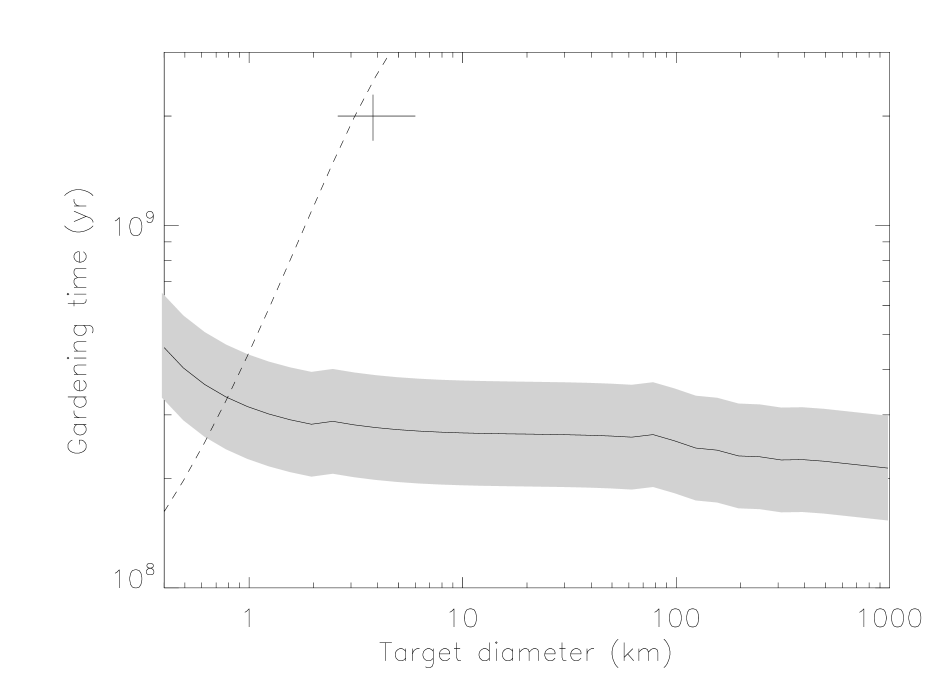
Figure 1:

Calculated gardening time (solid curve) from asteroid impact and cratering rates as a function of target diameter. The shaded region is our formal estimate of the statistical error on the gardening given the uncertainty on all the input parameters. The actual systematic error is much larger as discussed in the text. Our measured color-derived gardening time is the single data point in the upper left. The asteroid disruption lifetime is given by the dashed curve (Bottke et al. , 2005b, ). The histogram (right ordinate) shows the size distribution of all the asteroids used in this study assuming an albedo for the S-complex asteroids of 0.20.

Combining all the discussion in this section above we find that the characteristic gardening time from eq. 12 is given by

$$\tau_{g}(N(D),D_{T},Q_{S}^{*},v,\rho_{T},\rho_{I})\;\lower 2.0pt\hbox{$\,\buildrel\scriptstyle>\over{\scriptstyle\sim}\,$}\;\frac{9.8\times 10^{14}\;D_{T}^{2.067}}{\int_{\sim 0}^{D_{max}(Q_{S}^{*},v,\rho_{T},\rho_{I})}\;N(D)\;\biggl{(}\frac{D_{T}+D}{2}\biggr{)}^{2}\;D^{2.01}\;dD}.$$ (19)

Figure 1 provides our nominal estimate of the characteristic gardening time using $Q_{S}^{*}(D_{T})$ from Holsapple et al. , (2002), $v=5$ km/s (Bottke et al. ,, 1994), $\rho_{I}=\rho_{T}=$2.63 g cm^-3 (Hilton,, 2002; Fujiwara et al. ,, 2006) and $N(D)$ from Bottke et al. , 2005b . We find that the gardening time frame is a mild function of diameter, only 23% slower on small (1 km) asteroids than on large (100 km). The calculated resurfacing time for $D_{T}\sim 4$ km, the typical diameter of asteroids in our study, is $\sim 270$ My. Note that asteroids with diameters $\,\buildrel\scriptstyle<\over{\scriptstyle\sim}\,$700 m have disruption lifetimes shorter than either the calculated gardening time or the weathering time implying that few of them would be fully weathered or gardened. Since (25143) Itokawa is $\sim$535 m long it is unlikely to be completely reddened and Ishiguro et al. , (2007) provide evidence of some space weathering. Unfortunately, the three bvw filter bands used in situ on (25143) Itokawa are not comparable to the five SDSS ugriz filters and we cannot calculate $PC_{1}$ to determine where (25143) Itokawa’s color falls on our scale.

As new surveys detect asteroids of smaller diameters we may be able to discover this transition size, further constraining the weathering/gardening model. However, the asteroids in our sample have lifetimes $\lower 2.0pt\hbox{$\,\buildrel\scriptstyle>\over{\scriptstyle\sim}\,$}2$ Gy so their record of space weathering and gardening should not be distorted by an early demise.

The above result for the resurfacing time determined by impacts is compared to the gardening time determined via age-color data in §6.4.

4 Data acquisition and reduction

We observed or obtained spectra or photometry for ten asteroids within the four known sub-My clusters as shown in Table 1. The data came from three sources: 1) new spectra and photometry were acquired by our team using KeckII/ESI (Sheinis et al. ,, 2002), UH2.2 m/SNIFS (Lantz et al. ,, 2004) and IRTF/SpeX (Rayner et al. ,, 2003), 2) spectra were also provided by Mothé-Diniz and Nesvorný, (2008), hereafter referred to as MDN, and 3) we identified photometry for some sources from SDSS DR7 MOC4 (Parker et al. ,, 2008).

Asteroid	Observation (HST)	Source	Mag (H/V)	Type	Axis
(1270) Datura	2007 Oct 28	UH/SNIFS	12.5/17.1	Sl	2.234
(1270) Datura	2008 Mar 2	KeckII/ESI	12.5/16.5	Sl	2.234
(1270) Datura	2007 Nov 16	MDN	12.5/16.7	Sk	2.234
(90265) 2003 CL5	2007 Mar 15	MDN	15.4/19.3	Sq	2.235
(60151) 1999 UZ6	2007 Mar 15	MDN	16.1/20.5	Sk	2.235
(60151) 1999 UZ6	2001 Mar 18	SDSS	16.1/20.1	Sq/Sk	2.235
(203370) 2001 WY35	2007 Sep 2	MDN	17.6/21.5	O/Q	2.235
2003 UD112	2003 Sep 25	SDSS	18.4/20.0	Sq	2.233
(14627) Emilkowalski	2006 Oct 1	UH/SNIFS	13.1/16.6	T	2.598
(14627) Emilkowalski	2008 Apr 13	UH/SNIFS	13.1/17.3	T	2.598
(14627) Emilkowalski	2008 Apr 18	IRTF/SpeX	13.1/17.4	-	2.598
(14627) Emilkowalski	2004 Jan 27	SDSS	13.1/18.3	D	2.598
(16598) 1992 YC2	2007 Aug 17	MDN	14.7/20.3	Sq	2.621
(16598) 1992 YC2	2000 Jan 1	SDSS	14.7/17.0	S	2.621
(21509) Lucascavin	2006 Aug 1	UH/SNIFS	15.0/19.2	Sk	2.281
(21509) Lucascavin	2008 Apr 18	IRTF/SpeX	15.0/18.1	-	2.281
(180255) 2003 VM9	2008 Mar 2	KeckII/ESI	17.0/19.7	Sk	2.280
(209570) 2004 XL40	2007 Aug 20	MDN	17.1/20.4	Sq	2.281

Table 1:

Observations and basic properties of members of four sub-My old asteroid clusters adapted from Nesvorný et al. , (2006) and Nesvorný and Vokrouhlický, (2006). The four clusters are separated by table lines and named after the first object listed in each cluster. Dates of observation and the data source are listed in the second and third columns respectively. Absolute magnitude (H) is listed along with the apparent magnitude (V) on the date of observation from JPL, (2009). We have determined the taxonomic type based on the SMASS (Bus and Binzel,, 2002; Bus et al. ,, 2002) classification system as described in the text. The tight clustering in semi-major axis within each cluster is a consequence of their family membership.

Our spectroscopic reduction techniques for the new data followed generally accepted practices using standard IRAF and IDL procedures that are explained in detail in Willman et al. , (2008). Procedures applied to some of the spectrographic data that may not be standard include:

• using 2-D arc lamp spectra to create a transform map to straighten the 2-D asteroid and analog spectra.

• median-combining straightened dome flats into a column normalized master flat. i.e. the average of all pixels in any column (at the same wavelength) in the master dome flat was fixed at unity to correct for pixel-to-pixel variations in the quantum efficiency at all points on the CCD at the same wavelength.

• creating a water band model by dividing solar analog spectra from the same star that show the greatest difference in water band amplitudes. This allowed us to enhance the water bands for that solar analog. Combining such cases from different stars produced the master water band spectrum that allowed better cancellation of atmospheric water absorption bands redward of 800 nm (Bus and Binzel,, 2002).

• dividing the master water band spectrum into the asteroid spectrum and allowing the strength of the master to vary in order to minimize the distortion due to water bands. (Bus and Binzel,, 2002)

• binning the spectra into 10 nm bins in the manner of Bus and Binzel, (2002) such that the realized resolution was in the range $44\lesssim R\lesssim 92$ over the wavelengths spanning $440-920$ nm.

The spectral reduction procedures generally apply to UH2.2 m/SNIFS and IRTF/SpeX spectra although some steps were performed automatically by the SNIFS pipeline. The IRTF/SpeX data reduction is facilitated by an IDL based package called Spextool (Cushing et al. ,, 2004) which includes preparation of calibration frames, processing and extraction of spectra from science frames, wavelength calibration and flux calibration.

We used the solar colors of Blanton et al. , (2007) in our $PC_{1}$ and $PC_{2}$ measurement and absolute magnitude corrections for $u$ and $z$ bands from SDSS, 2006b .

To combine the spectral results with the photometric results described below in a consistent manner we required a method to calculate $PC_{1}$ (eq. 1) for the spectra. To do so we relied on the relationship between spectral slope $s$ and $PC_{1}$ derived by Willman et al. , (2008). They used a sample of 133 asteroids common to both SMASS and the SDSS $3^{rd}$ Data Release to determine that

$$PC_{1}=(0.87\pm 0.02)\times(s/{\mu\rm{m}}^{-1})+(0.082\pm 0.012)$$ (20)

where the SMASS slope $s$ is determined over the wavelength range from $0.44-0.92\;\mu$m as the best fit line pivoting through the normalization point at 0.55 µm.

$Asteroid$		$u$	$g$	$r$	$i$	$z$
1986	JN1	18.40 $\pm$ 0.03	16.95 $\pm$ 0.03	16.46 $\pm$ 0.02	16.31 $\pm$ 0.01	16.24 $\pm$ 0.02
2000	WX167	21.05 $\pm$ 0.08	19.65 $\pm$ 0.02	19.07 $\pm$ 0.02	18.92 $\pm$ 0.02	18.82 $\pm$ 0.04
2001	MD30	18.95 $\pm$ 0.07	17.62 $\pm$ 0.02	17.10 $\pm$ 0.01	16.93 $\pm$ 0.01	16.89 $\pm$ 0.15
2000	NZ10	20.15 $\pm$ 0.06	18.50 $\pm$ 0.02	17.79 $\pm$ 0.02	17.61 $\pm$ 0.01	17.63 $\pm$ 0.03
2002	AL80	22.51 $\pm$ 0.30	20.66 $\pm$ 0.03	20.02 $\pm$ 0.02	19.83 $\pm$ 0.03	19.85 $\pm$ 0.07
1999	KF	21.21 $\pm$ 0.12	19.46 $\pm$ 0.02	18.77 $\pm$ 0.02	18.59 $\pm$ 0.02	18.58 $\pm$ 0.04
2002	GP75	22.44 $\pm$ 0.27	21.01 $\pm$ 0.03	20.36 $\pm$ 0.03	20.27 $\pm$ 0.03	20.25 $\pm$ 0.11
2006	AL54	21.97 $\pm$ 0.20	20.54 $\pm$ 0.03	19.88 $\pm$ 0.02	19.68 $\pm$ 0.02	19.66 $\pm$ 0.06
1962	RD	17.32 $\pm$ 0.05	15.54 $\pm$ 0.03	14.88 $\pm$ 0.03	14.60 $\pm$ 0.02	14.63 $\pm$ 0.02
1997	CT16	21.14 $\pm$ 0.09	19.37 $\pm$ 0.02	18.59 $\pm$ 0.02	18.43 $\pm$ 0.01	18.44 $\pm$ 0.04
2000	RV55	22.07 $\pm$ 0.27	20.31 $\pm$ 0.03	19.60 $\pm$ 0.02	19.36 $\pm$ 0.03	19.41 $\pm$ 0.05
2004	RJ294	23.27 $\pm$ 0.54	21.77 $\pm$ 0.06	21.09 $\pm$ 0.05	20.93 $\pm$ 0.05	21.00 $\pm$ 0.19
2003	SC7	22.21 $\pm$ 0.18	20.60 $\pm$ 0.02	20.03 $\pm$ 0.02	19.77 $\pm$ 0.03	20.15 $\pm$ 0.11
2000	GQ113	20.52 $\pm$ 0.05	18.89 $\pm$ 0.03	18.27 $\pm$ 0.02	18.07 $\pm$ 0.02	18.24 $\pm$ 0.02
1983	WM	19.59 $\pm$ 0.03	17.78 $\pm$ 0.01	17.07 $\pm$ 0.01	16.87 $\pm$ 0.01	17.10 $\pm$ 0.02
2003	YK39	22.53 $\pm$ 0.31	20.56 $\pm$ 0.03	19.83 $\pm$ 0.03	19.77 $\pm$ 0.02	19.81 $\pm$ 0.07
1999	TE221	20.71 $\pm$ 0.08	19.21 $\pm$ 0.02	18.66 $\pm$ 0.02	18.46 $\pm$ 0.02	18.75 $\pm$ 0.04
2000	LU15	21.50 $\pm$ 0.11	19.76 $\pm$ 0.02	18.99 $\pm$ 0.02	18.88 $\pm$ 0.02	19.39 $\pm$ 0.05
2001	XH209	23.30 $\pm$ 0.56	20.58 $\pm$ 0.04	19.82 $\pm$ 0.02	19.57 $\pm$ 0.04	19.60 $\pm$ 0.10

Table 2:

$ugriz$ photometry for 19 asteroid pair members from SDSS DR7 MOC4. The two objects shown in bold constitute the only complete pair.

Table 2 provides multiband photometry shown in Figure 2 from the SDSS DR7 MOC4 for 19 members of 18 pairs from the sub-set of non-family pairs (Pravec et al. ,, 2009). Only one pair had observations of both members available in the SDSS data set.

Figure 2:

SDSS five-filter $ugriz$ photometry for 19 objects common to the dynamically young pair members and also in the SDSSDR7 MOC 4. The approximate band centers and widths for all five filters are shown at the bottom of the Figure. The SDSS filter measurements have been connected by lines to simulate full spectra and are normalized to 1.0 at 0.55 $\mu$m.

5 Taxonomic type identification

While there has been recent and interesting progress in automated taxonomic classification from asteroid photometry or spectrometry(e.g.  Marzo et al. ,, 2009; Misra & Bus,, 2008; Bus & Binzel,, 2000; Howell et al. ,, 1994) the process is still as much an art as science. In an attempt to be consistent (if not rigorous) in our taxonomic classifications we developed and employed three closely related methods: 1) taxonomic fitting 2) principal color component space location and 3) visual assessment. Our classifications with the three methods were correlated with each other and with accepted taxonomic classifications for known objects but were not identical.

The first method selects the best taxonomic ‘fit’ for an object’s photometry to each SMASS spectral type $j$ according to the spectral difference

$$\Delta_{j}^{2}=\sum_{i=ugriz}\frac{(A_{i}-S_{ij})^{2}}{(\sigma_{A_{i}}^{2}+\sigma_{S_{ij}}^{2})}$$ (21)

where $A_{i}$ and $S_{ij}$ are the asteroid and SMASS (Bus and Binzel,, 2002) standard mean flux in band $i$ respectively and $\sigma_{A_{i}}$, $\sigma_{S_{ij}}$ are the errors on the asteroid and SMASS magnitudes in the same band. The errors on the mean SMASS spectra range from 0.01 - 0.06 and average about 0.03.

One complication with employing this technique is that the $u$ band center is at 3557 Å while SMASS spectra extend only over the range 4400-9200 Å. Therefore, to compare SMASS spectra to the SDSS filter bands in eq. 21 (and in the other two methods described below) we performed a linear extrapolation of the SMASS spectra to the $u$ band central wavelength from the $g$ and $r$ band centers. We tested several other methods of extrapolating to the $u$ band including a quadratic extrapolation to $u$ using $g$, $r$ and $i$ bands or a quadratic extrapolation using all four of $g$, $r$, $i$ and $z$ bands. We also tested the result when we simply ignored the $u$ band. None of these techniques gave type identifications as good as the simple linear extrapolation from $g$ and $r$ even though the linear approximation glosses over a possible inflection point at 0.42 $\mu$m (Ishiguro et al. ,, 2007).

The second method selects the taxonomic type with the smallest distance in principal component color space ($PC_{1}$,$PC_{2}$) between the mean for each SMASS type $j$ and the object of interest as illustrated in Figure 3. We parametrize the distance $R_{j}$ simply as

$$R_{j}^{2}=\Delta PC_{1j}^{2}+\Delta PC_{2j}^{2}$$ (22)

where $\Delta PC_{1j}$ and $\Delta PC_{2j}$ are the difference in $PC_{1}$ and $PC_{2}$ between the object and the SMASS class $j$ band average.

Figure 3:

$PC_{2}$ vs. $PC_{1}$ for eighteen pair members having SDSS $ugriz$ photometry are shown as circles. Filled/open circles lie inside/outside the region generously defining the S-complex. Mean locations for SMASS classes are indicated by their taxonomic identification code. We assign Q-class objects to the S-complex as discussed in the text.

Finally, the third method was a traditional visual assessment of the asteroid’s spectrum. This time-tested method incorporates elements of both methods discussed above, takes into consideration the extrapolation to $u$ band and takes advantage of human perception for overall shape matching. In this method, more weight was given to the degree of shape matching than to minimizing band center differences.

In the end, we found that the top two candidate SMASS subclasses from each of the three methods were consistent and that visual assessment provided the the most reliable taxonomic classification method.

6 Results and discussion

6.1 Sub-My cluster member taxonomy

We observed the brightest member of each of the four sub-My clusters to identify their taxonomic type. The spectra or multiband photometry for each object are shown in Figure 4. (1270) Datura, (16598) 1992 YC2 and (21509) Lucascavin all show classic S-complex characteristics in the visible — a 0.75 $\mu$m peak and a 1.0 $\mu$m absorption band. Datura also shows an inflection near 0.55 $\mu$m indicating a fresher surface relative to older S asteroids with smoother spectra (Ishiguro et al. ,, 2007; Hiroi et al. ,, 2006).

(21509) Lucascavin also shows the 2.0 $\mu$m band typical of pyroxene. Using the techniques described in §5 we identify (1270) Datura as an Sk, close to Mothé-Diniz and Nesvorný, (2008)’s identification of Sl, (21509) Lucascavin also as an Sk, and (16598) 1992 YC2 as member of the S-complex. Our visible and IR spectra of (14627) Emilkowalski does not show the 1.0 and 2.0 $\mu$m absorption bands typical of the S-complex and we classify it as T type. As our space weathering model only applies to asteroids within the S-complex we ignore (14627) Emilkowalski for the remainder of this work.

Figure 4:

Visible and near IR spectra of (14627) Emilkowalski and (21509) Lucascavin obtained with UH2.2 m/SNIFS and IRTF/SpeX, (1270) Datura visible spectrum obtained with UH2.2 m/SNIFS, and SDSS (16598) 1992 YC2 photometry. The spectrum of (14627) Emilkowalski is normalized to 1.0 at 0.55 $\mu$m and the others are offset vertically. The gap at $\sim 1.9\mu$m results from removing a sky absorption band. The (1270) Datura visible spectrum, (14627) Emilkowalski and (21509) Lucascavin IR spectra are all smoothed fits to the data (causing a spurious mismatch to the visible spectrum), the others are binned.

It is unsurprising that (1270) Datura and (21509) Lucascavin were identified in the S-complex as both clusters are located in the inner main belt which is dominated by S-complex asteroids. Similarly, (14627) Emilkowalski and (16598) 1992 YC2 are located in the middle of the main belt where X and S-complex types are common.

Having identified three of the sub-My clusters within the S-complex for which we intend to examine the effects of space weathering and gardening we obtained data for eight of the cluster members as provided in Table 3.

Cluster	Asteroid	Source	Slope	$PC_{1}$	Age
			(Reflectance/$\mu$m)		(kyr)
	(1270) Datura	MDN	$0.355$	$0.391$	$530\pm 20$
	(1270) Datura	this work	$0.382$	$0.414$	”
Datura	(203370) 2001 WY35	MDN	$-0.155$	$-0.053$	”
	(60151) 1999 UZ6	MDN	$0.606$	$0.609$	”
	(90265) 2003 CL5	MDN	$0.205$	$0.260$	”
			mean	$0.305\pm 0.278$
	(21509) Lucascavin	this work	$0.476$	$0.496$	$300-800$
Lucascavin	(209570) 2004 XL40	MDN	$0.314$	$0.355$	”
	(180255) 2003 VM9	this work	$0.327$	$0.366$	”
			mean	$0.406\pm 0.078$
1992 YC2	(16598) 1992 YC2	MDN	$0.083\pm 0.02$	$0.155\pm 0.027$	$135-220$
			Sample Mean	$0.36\pm 0.07$	$511\pm 10$

Table 3:

Derived color data and age estimates (Nesvorný et al. ,, 2006; Nesvorný and Vokrouhlický,, 2006) for members of three S-complex sub-My clusters. $PC_{1}$ was calculated using eq. 20. Errors on the slope and $PC_{1}$ are not included as the error on the family’s color is dominated by the distribution of $PC_{1}$ values within a cluster. The errors on cluster means are standard deviations except for (16598) 1992 YC2 for which the measurement error is provided since it was the only object observed in the cluster. The Sample Mean includes all eight cluster members with the error on the mean.

6.2 Taxonomy and orbit distribution of asteroid pair members

$Ast_{1}$		SMASS	Tholen	Quality	$Ast_{2}$		a	e	i	$H_{1}$	$H_{2}$
							(AU)		(degrees)
1986	JN1	X, Xe	EMP, EMP	good	2001	XO105	$1.946$	$0.0601$	$23.710$	$13.5$	$17.4$
2000	WX167	Xe, T	EMP, T	fair	2007	UV	$1.909$	$0.0613$	$23.096$	$16.2$	$17.1$
2001	MD30	Xe, X	EMP, EMP	fair	2004	TV14	$1.938$	$0.0886$	$19.987$	$14.9$	$17.2$
2000	NZ10	L, Sl	S, S	good	2002	AL80	2.287	0.1801	4.097	14.1	16.2
2002	AL80	Sl, S	S, S	good	2000	NZ10	”	”	”	16.2	14.1
1999	KF	L, Sl	S, S	good	2008	GR90	$2.327$	$0.2339$	$1.777$	$15.0$	$17.2$
2002	GP75	L, S	S, S	good	2001	UR224	$2.340$	$0.1727$	$3.865$	$15.7$	$17.2$
2006	AL54	L, Sl	S, S	good	2000	CR49	$2.272$	$0.1763$	$4.591$	$16.8$	$14.3$
1962	RD	Sl, Ld	S, S	good	1999	RP27	$2.198$	$0.1775$	$1.129$	$13.1$	$15.3$
1997	CT16	Sl, Sa	S, S	good	2002	RZ46	$2.186$	$0.1672$	$4.599$	$15.4$	$16.4$
2000	RV55	Sl, Sa	S, S	good	2006	TE23	$2.657$	$0.1026$	$2.245$	$14.9$	$16.8$
2004	RJ294	S, Sr	S, S	good	2004	GH33	$2.268$	$0.0981$	$4.238$	$18.2$	$16.7$
2003	SC7	Sk, K	S, S	good	1998	RB75	$2.264$	$0.1114$	$7.263$	$16.6$	$14.6$
2000	GQ113	Sq, Sk	S, S	good	2002	TO134	$2.324$	$0.1319$	$5.515$	$14.4$	$16.3$
1983	WM	Sr, Sa	S, S	good	1999	RC118	$2.320$	$0.0790$	$5.726$	$13.7$	$14.6$
2003	YK39	Sr, Q	S, Q	good	1998	FL116	$2.187$	$0.0845$	$3.736$	$18.3$	$15.0$
1999	TE221	Q, V	Q, V	fair	2001	HZ32	$2.308$	$0.1540$	$5.642$	$16.5$	$15.0$
2000	LU15	V, Q	V, Q	good	1992	WJ35	$2.313$	$0.0701$	$5.742$	$16.1$	$13.7$
2001	XH209	A, Sa	A, S	good	2004	PH	$2.401$	$0.2150$	$3.638$	$15.6$	$16.4$

Table 4: Asteroid pair member data for objects appearing in SDSS DR7 MOC4. We determined SMASS taxonomy for $Ast_{1}$ using $ugriz$ photometry from SDSS DR7 MOC4 as described in the text. The first and second ranked SMASS classes (§5) are provided along with the corresponding Tholen classes and an assessment of that match’s quality (degree of identification certainty). Semi-major axis (a), eccentricity (e), inclination (i) and absolute magnitudes ($H_{1}$,$H_{2}$) of both asteroids are from Vokrouhlický and Nesvorný, (2008); Pravec et al. , (2009). Members shown in bold constitute the only complete pair.

None of the members of 36 non-family asteroid pairs (Pravec et al. , (2009); Vokrouhlický and Nesvorný, (2008), §1 describes paired asteroids’ discovery based on similar orbits.) are available in either the SMASSI or SMASSII (Bus and Binzel,, 2002) spectra databases or the Eight Color Asteroid Survey (ECAS) (Tholen,, 1989). This is unsurprising considering that the pair members are considerably smaller than the typical asteroid in those surveys. However, the 19 pair members identified in Table 4 were found in the SDSS MOC4 (Parker et al. ,, 2008) from which we obtained the five-filter solar-corrected $ugriz$ photometry in Table 2.

Most of the pair members are located in the inner main belt in a region dominated by S-complex asteroids. Their SDSS photometry indicate that they belong to various taxonomic types typical of the inner belt including L, S and V classes. Our formal identification of the pair member’s taxonomy using the methods described in §5 are provided in Table 4 which shows that we have identified 14 of the 19 pair members with the S-complex in which we also include L-class and Q-class. We will examine the colors of these asteroids in the context of our space weathering model later in this section. We also identified three X-class, one V-class, and one A-class asteroid.

The taxonomic variety of the pair members is also represented in Figures 3 and 6 which shows that their $PC_{1}$ color distribution is narrower than the full span of SMASS classes while the distribution of their $PC_{2}$ values extends beyond the SMASS class range. Several pair members have $PC_{2}<-0.4$. Since $PC_{2}$ corresponds roughly to a spectrum’s curvature this indicates an unusually convex spectrum. A couple pair members lie close to the V-class region while only one lies in the C-complex. We believe that the dearth of C-complex objects is an observational artifact because pair members tend to be small and would be difficult to detect with the low albedo of C-complex members in the outer belt.

The assignation of 1999 TE₂₂₁ to the Q class is important to our space weathering analysis since it has been suggested (Binzel et al. ,, 2004) that Q-class objects are actually very young, essentially unweathered, S-complex asteroids. Thus, we assume that it is a particularly young member of the S-complex with a deep $1\mu$m band as has been predicted for young S-complex asteroids. However, in osculating element space it is located close to 2000 LU₁₅, another member of one of our asteroid pairs from table 4 that we assigned to the V-class. Both the asteroids lie close to the edge of the Vesta family region as shown in fig. 3 (again, in osculating elements). This opens the possibility that 1999 TE₂₂₁ could be a Vestoid with a slightly shallower $1\mu$m absorption band.

To confirm our Q-class identification for 1999 TE₂₂₁ and as an additional check on our type-identifications we examined whether the pair members are of taxonomic types typical of their orbit element phase space region. To do so we identified each pair member’s five nearest orbit element neighbors (using the $D$-criterion of Nesvorný et al. , (2005)) in the set of 1175 objects from SMASS that also have osculating orbital elements in AstDyS, (2008). We found that 17 out of 19 pair members match their nearest neighbor’s complex suggesting that our identification methods identify the right complex $\sim 90$% of the time and that the pair members are representative of the composition of the main belt region in which they are located.

As mentioned earlier, this test was particularly important for the cases of 1999 TE₂₂₁ and 2000 LU₁₅ as both lie on the periphery of the Vesta family region. We identify the $1^{st}/2^{nd}$ most likely types for these two objects as Q/V and V/Q respectively. 1999 TE₂₂₁’s five nearest neighbors include four in the S-complex with one being a Sq and none in the V-class. On the other hand, 2000 LU₁₅ has three V-class neighbors. This supports our ability to reliably distinguish Q from V. Remember that we place the Q-class within the S-complex and, since 1999 TE₂₂₁ is by far the bluest member of the S-complex pair members, its inclusion in our analysis could have a substantial impact on the mean $PC_{1}$ of the pair members and on our measurement of the space weathering rate of S-complex asteroids. The effect of including or excluding 1999 TE₂₂₁ in our analysis is described later.

Our interest in and utilization of the asteroid pairs for the purpose of measuring young asteroid surface ages assumes that the pair members are genetically related and fissioned by some as yet undefined process $<0.5$ My ago (Vokrouhlický and Nesvorný,, 2008). If the members of a pair are genetically related asteroids then our expectation is that they will display nearly identical spectra. Only one complete pair (2000 NZ₁₀ and 2002 AL₈₀, see Table 4) was identified among the 19 pair members available in the SDSS MOC4. Figure 5 shows that the colors of the two objects match and therefore supports a genetic origin of the pair. Using the taxonomic identification methods of §5 we find that 2000 NZ₁₀ is SMASS L-class and 2002 AL₈₀ is Sl-class - adjacent classes in $PC_{2}$ vs. $PC_{1}$ color space as shown in Figure 3. Thus, this one line of evidence suggests that asteroid pairs are genetically related.

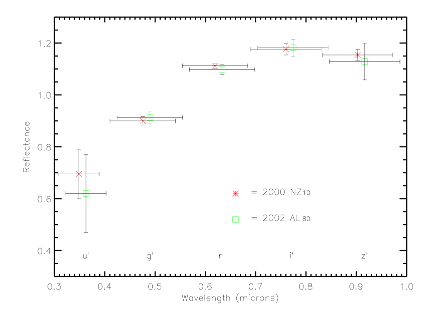
Figure 5:

SDSS filter photometry for both members of the only complete dynamical pair in the MOC4. The central wavelength for each data point corresponds to the band centers for the $ugriz$ filters except for a small horizontal offset for clarity while their width represents the band pass. The data is normalized such that a straight line between the $g$ and $r$ data points passes through unity at 0.55 $\mu$m.

Having established the taxonomic composition of the asteroid pairs and their likely genetic relationship we would like to examine their taxonomic-orbit distribution — does the pair member taxonomy match that of their neighbors in orbit element space? The answer to this question could shed light on the relative internal strengths of the different types or provide information on the mechanism for asteroid pair creation. i.e. if C-complex asteroids split into pairs more frequently it could imply that they are weaker than other types or that the pair formation mechanism acts more efficiently on them. Unfortunately, answering this question is beyond the scope of this work and we leave it to the future. Instead, we make a couple simple observations on the pair’s orbit element distribution.

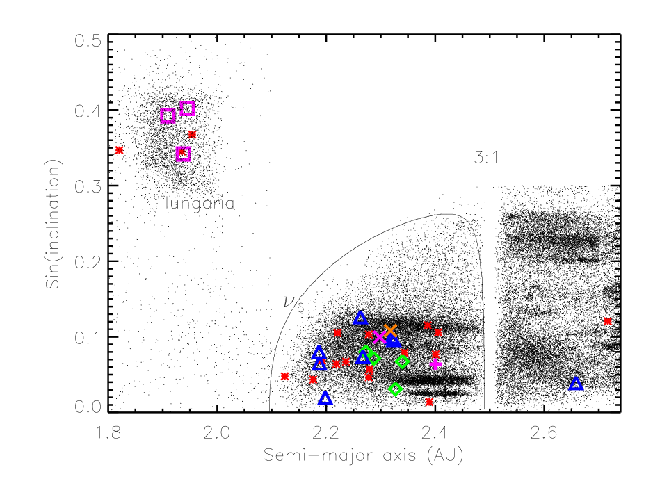
Figure 6:

Osculating $\sin$(inclination) versus semi-major axis for 36 pair members (large colored points) superimposed on the proper element distribution for main belt asteroids identified in the SDSS MOC4 (black dots). For semi-major axis $<2.1$ AU we show osculating elements for main belt asteroids from Astorb (Astorb,, 2008). The 18 distinct pair members with SDSS photometry were identified as the following types: violet squares are X-complex, blue triangles are S-complex, green diamonds are L-complex, the orange $\times$ is V-class, the fuchsia $\times$ is Q-class, and the fuchsia $+$ is A-class. The 18 red asterisks represent pairs for which neither member is present in the SDSS MOC4. The $\nu_{6}$ and 3:1 resonances are shown for orientation along with the Hungaria family region.

The axis-inclination structure of the main belt and the pairs is shown in Figure 6 revealing that the 36 pairs are distributed in two clumps; a high inclination clump inside 2.0 AU within the Hungaria family region, a group dynamically protected from perturbations by Mars via their high inclination, and a clump on the inner edge of the main belt with 2.1 AU$\lower 2.0pt\hbox{$\,\buildrel\scriptstyle<\over{\scriptstyle\sim}\,$}a\lower 2.0pt\hbox{$\,\buildrel\scriptstyle<\over{\scriptstyle\sim}\,$}$ 2.4 AU. There are also two outliers in the middle belt with semi-major axes in the range 2.65 AU$<a<$ 2.75 AU. That most of the pairs are located in the innermost main belt is almost certainly an observational selection effect — asteroid pairs are composed of small asteroids that are only visible when they are located close to the Earth i.e. in the inner main belt.

The Hungaria clump includes six pairs of which three have SDSS photometry that we identify as (SMASS) X-complex asteroids — consistent with Gradie and Tesdesco, (1982)’s claim that roughly 70% of the asteroids in the Hungaria region are Tholen E or R class (the Tholen E class is contained within the SMASS X-complex). Thus, our identification of three SDSS X-complex members in the region is unsurprising and provides further support for our taxonomic classification techniques.

6.3 Space weathering on sub-My clusters and asteroid pairs

Figure 7 combines our previous work (Willman et al. ,, 2008) with the new color-age data in this work for S-complex asteroids in three sub-My clusters and eleven sub-My asteroid pairs. The mean $PC_{1}$ for the three sub-My clusters is $0.36\pm 0.07$ — within 1$\sigma$ of Willman et al. , (2008)’s predicted color of $PC_{1}=0.31\pm 0.04$ for the clusters’s mean age of $440\pm 60$ kyr. The good agreement with the prediction lends confidence to the space weathering model which now agrees with the cluster color-age data over five orders of magnitude in age in the decades from $10^{5}-10^{10}$ years.

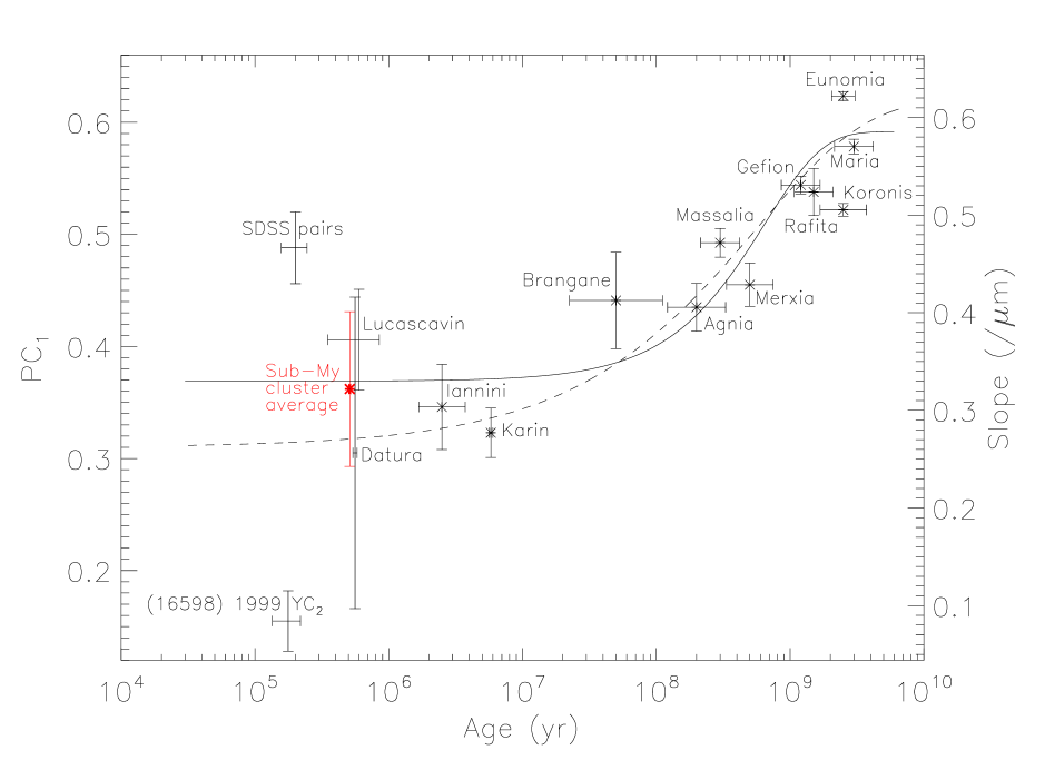
Figure 7:

$PC_{1}$ color and dynamically determined ages for S-complex asteroid families adapted from Willman et al. , (2008). (The corresponding spectral slope is shown on the right.) The dashed curve represents their space weathering model (eq. 3) extrapolated to the sub-My region. Three S-complex sub-My clusters ((1270) Datura, (21509) Lucascavin, (16598) 1992 YC2) are shown individually and with their mean value indicated by the red ‘Sub-My cluster average’ data point. The solid curve represents the dual weathering/gardening model fit to the family data including the sub-My cluster point. The ‘SDSS pairs’ point represents the average color of 12 unique S-complex sub-My pairs found in SDSS DR7 MOC4. Errors are standard errors on the mean except for (16598) 1992 YC2, a single object, for which we provide the measurement error.

However, the weighted mean $PC_{1}=0.49\pm 0.03$ color (the error is weighted error on the mean) for the S-complex young pairs is over $5\sigma$ redder than predicted by Willman et al. , (2008). Excluding the Q-type pair member 1999 TE₂₂₁ discussed in §6.2 increases the mean $PC_{1}$ to $0.54\pm 0.04$ and the discrepancy to over $7\sigma$. The very young asteroid pairs clearly do not follow the space weathering function proposed by Willman et al. , (2008).

The disparity may be explained in a number of ways: 1) the asteroid pairs do not represent a recent breakup of a parent body and are not genetically related or 2) the asteroid pairs are the result of a recent breakup but with only partial resurfacing which did not ‘reset’ the space weathering clock or 3) the space weathering model of Willman et al. , (2008) is either too simplistic or wrong. We examine each of these scenarios in turn:

1. We consider it unlikely that the asteroid pairs are not genetically related for two reasons. First, the pairs were specifically selected (Vokrouhlický and Nesvorný,, 2008) because they are statistically likely to be related asteroids. Furthermore, the colors of the pair for which both members exist in the SDSS MOC4 agree extremely well (see Fig. 5). While asteroids that inhabit the same region of the main belt often have similar colors the scale of agreement in both the orbit and colors argues persuasively for a genetic link between the pair members.

2. Some pair formation scenarios may not be as violent as the formation of large asteroid families through the catastrophic disruption of a parent body and may not reset the entire surface to zero age. Vokrouhlický and Nesvorný, (2008) cite three possible methods of forming pairs: catastrophic collision followed by fragment reaccumulation into binary orbits (e.g.  Durda et al. ,, 2004; Nesvorný et al. ,,, 2006), YORP induced rubble pile spin-up leading to calving of the secondary (e.g.  Walsh et al. ,, 2008), or YORP induced angular acceleration of contact binaries leading to their separation (e.g.  Merline et al. ,, 2002; Pravec et al. ,, 2009; Durda et al. ,, 2004). The first scenario will ‘reset’ the age of the entire surface of both the primary and secondary. The third mechanism might leave large portions of the surface undisturbed since the only portion that is necessarily exposed is the binary contact region. It is unclear how much of the surface would be affected by the second scenario. Therefore there is a clear distinction between the possible formation mechanisms of pairs and larger groupings. Asteroid families and clusters with more than two members form only by the first catastrophic collisional scenario while pairs can also form by the two variations on YORP spin-up. This yields at least one pair formation scenario that could leave some of the members’ surface undisturbed. In this case the globally averaged surface color would correspond to a misleading age somewhere between fresh surface and the age of the parent body’s surface. Taking the color of the pairs at face value and interpreting it in the framework of the Willman et al. , (2008) space weathering model indicates an average surface age of $\sim 440$ My — over 1000$\times$ older than their dynamical age. If we assume that the original parent body’s surface was reddened to saturation prior to separation, and taking the dynamical ages of $<500$ kyr for the pairs at face value such that freshly exposed surface is essentially unweathered, then $\sim 64$% of the surface must be disturbed in the pair separation process. Considering that it is unlikely that the surface was fully weathered prior to separation allows us to set an upper limit on the fraction of disturbed surface at $\lesssim 64$%. (Excluding the Q-type object 1999 TE₂₂₁ only changes the upper limit to $\lesssim 48$%.) A gentle binary separation due to slow YORP spinup may be consistent with this scenario. Indeed, Pravec et al. , (2009) also provide evidence from reconstruction of the initial configuration of the 6070-54827 pair and rotation rate observations that the non-family pair formation process is a gentle event. If we envision a bi-lobed asteroid gradually accelerating in angular velocity and finally fissioning at the neck that joins the lobes then it seems reasonable that the portion of disturbed surface would be $\lesssim 64$%. In the binary/pair formation mechanism proposed by Walsh et al. , (2008, 2006) an asteroid’s polar surface material migrates to the equator as the object’s rotation rate increases and eventually flies into orbit around the parent body where it reaccumulates into a satellite. The primary and satellite eventually separate and their orbits evolve dynamically. Our impression is that this model would generate fresh (blue) surface on both the primary and satellite in conflict with our observation of reddish surfaces on the asteroid pairs. However, it is not difficult to envision a slow migration process that allows material to weather on the primary’s surface before being shed and accumulating into a secondary object.

3. It is possible that the space weathering model of Willman et al. , (2008) that built upon the earlier work of Nesvorný et al. , (2005) and Jedicke et al. , (2004) is simply wrong; that the apparent change in color of S-complex asteroids with age is a statistical fluke or due to some other underlying effect (though obvious possibilities were considered in detail in the early works). However, Parker et al. , (2008) confirm the weathering effect in an independent updated analysis of the SDSS DR7 MOC4 data. We consider it more likely that the space weathering mechanism is more complicated than simply affecting the average spectral slope (or $PC_{1}$) as a function of time. For instance, it is well known that space weathering affects not only the slope of the spectrum but also the depths of the 1 $\mu$m and ultraviolet absorption bands and the surface albedo. We consider it not only possible but likely that these effects occur during space weathering at different rates. The apparent redness of the young asteroid pair members relative to the expectation of the simplistic space weathering model could indicate that a ‘fast’ space weathering process takes place in $\lesssim 10^{5}$ years. However, this scenario requires a rather contrived sequence of events. Consider the three color change processes: decreasing depth of the ultraviolet band shortward of 0.4 $\mu$m, decreasing depth of the 1 $\mu$m absorption band and continuum reddening between these two bands. The first process is the only one that produces a bluer color. Therefore, accounting for the anomalous redness of the pair members requires the unlikely scenario that one of the latter two processes dominate on short time scales which is then belatedly overwhelmed by the first process which is then finally dominated by the third.

Given the disagreement between the asteroid pair color-age and the Willman et al. , (2008) space weathering model, and considering our enumerated arguments above, we continue with our analysis under the assumption that we can ignore the colors of the asteroid pairs in this new determination of the space weathering and gardening rates.

First, we fit all the S-complex color data including the sub-Myr clusters but not the asteroid pairs to the ‘old’ space weathering function of eq. 3. Considering the good agreement between the predicted (Willman et al. ,, 2008) and observed colors of the sub-Myr cluster members it is unsurprising that the fit including the new data matches the previous fit in all four parameters to within 1-$\sigma$ with $PC_{1}(0)=0.34\pm 0.02$, $\Delta PC_{1}=0.28\pm 0.05$, $\tau=700\pm 270$ My, $\alpha=0.58\pm 0.17$. However, as we observed in Willman et al. , (2008), fitting the color-age data to the form of eq. 3 suffers from multiple and wide minima in the fit-parameter space. Furthermore, the function does not explicitly separate the weathering and gardening effects.

On the other hand, we found that fitting the same color-age data to our new function that incorporates both space weathering and gardening (eq. 8) is better behaved because the solution space does not show multiple local $\chi^{2}$ minima. The best fit (lowest $\chi^{2}$) including the sub-My clusters (but, again, not the asteroid pair colors) yields $PC_{1}(0)=0.37\pm 0.01$, $\Delta PC_{1}=0.33\pm 0.06$, $\tau_{w}=960\pm 160$ My, $\tau_{g}=2000\pm 290$ My as shown by the solid curve in Figure  7.

Note that it is not correct to compare the new $\tau_{w}$ or $\tau_{g}$ to the old $\tau$ value because of the complicating and non-physical use of $\alpha$ in the generalizing exponent in the old functional form. In essense, the ‘old’ value was an effective weathering time that combined the effects of both regolith gardening and weathering. Since the effective weathering time can be shown to be equivalent to the time corresponding to the inflection point on the new weathering function, Figure 7 shows that the two models are in good agreement.

The old and new $\Delta PC_{1}$ are not strictly comparable either. Formerly in the weathering only case the entire surface would eventually reach the color $PC_{1}=PC_{0}+\Delta PC$. The weathering/gardening case will produce a lower equilibrium value with $PC_{1}<PC_{0}+\Delta PC$.

The new space weathering-only time frame of $\sim$1 Gy is consistent with the ‘slow weathering’ measured in lab-based measurements as discussed in the introductions. The ‘slow’ school includes our result of $\sim$1 Gy based on space observations of S-complex families, Sasaki et al. , (2001)’s equivalent value of 700 My at 2.6 AU based on pulsed-laser irradiated silicate pellets, and Pieters et al. , (2000)’s estimate of $100-800$ My for lunar surfaces based on crater counts and spectra and color-terrain correlations on (243) Ida (Veverka et al. ,, 1996). But these slow space weathering results disagree with the ‘fast weathering’ school that includes lab-based ion irradiation results from Vernazza et al. , (2009) ($\,\buildrel\scriptstyle<\over{\scriptstyle\sim}\,$ 1 My) and Loeffler et al. , (2009)’s ($\sim$ 5 kyr), and Takato, (2008)’s $<$450 kyr time scale based on a shallow 1 $\mu$m absorption band observed on (1270) Datura. We do not have an explanation for the discrepancy between the fast and slow weathering results.

6.4 Gardening Time

In §3 we calculated the gardening time for asteroid regolith as a function of target diameter as shown in Figure. 1. Over a broad range of asteroid sizes the gardening time scale is $200-300$ My years. This result is in dramatic disagreement with a similar calculation by Melita et al. , (2009) that was based on a collisional cratering model by Gil-Hutton and Lazzaro, (2002) and yielded a time scale of 2000 years for resurfacing Trojan asteroids. It is difficult to reconcile the two results that differ by five orders of magnitude. Two factors that we are aware of that explain some of the discrepancy are 1) that they used a Trojan impact probability double that of the main belt and 2) the slope of the Trojan size-frequency distribution was assumed to be $-3$ whereas the data we used had slope of $\sim-2.20$ appropriate to the main belt (Bottke et al. , 2005b, ). But these two differences only account for a fraction of the difference between our results.

Figure 1 also shows that our measured gardening rate from the S-complex asteroid color-age relationship is an order of magnitude different from our calculated rate based on impacts. Is it possible to reconcile this difference?

There is considerable uncertainty in the various terms involved in calculating the impact gardening time from eq. 19 but we have done our best to select the best contemporary values in each case. While the gray region on the figure represents the formal 1-$\sigma$ error on the calculation based on the reported errors on each input quantity there is considerable unreported systematic error in the calculation associated with its sensitivity to the input parameters and functions. In particular, we examined the sensitivity of the calculation to the:

• asteroid size frequency distribution, $N(D)$

• specific shattering energy function, $Q_{S}^{*}$, that determines the largest non-disruptive impactor (we used the Melosh, (1997) function as a comparison),

• impact speed and,

• $D_{min}$, the smallest impactor that creates ejecta

In each case we varied the input parameter or function over a range of of 2 to 4 in each direction. In most cases the gardening rate for large target objects is only slightly affected. The rate for objects $\sim$1 km diameter changed by a factor of about two or slightly more. The two most important factors in determining the gardening rate are 1) $D_{min}$ and 2) the amount of area covered by crater ejecta. Increasing $D_{min}$ or decreasing the ejecta area coverage both work to increase the gardening timescale. Leaving all other parameters at their nominal values, increasing $D_{min}$ to $\sim$30 m is sufficient to increase the gardening time to our measured value of $\sim$2 Gy. A similar result is obtained by decreasing the diameter of the ejecta field by a factor of two (the affected area by a factor of four).

In a related observation, Chapman, (2005) and others note the unexpected paucity of craters $<$200 m diameter on (433) Eros. Taken at face value the observation would imply a deficit of impactors $\lesssim 20$ m in diameter but O’Brien, (2009) has shown that no such deficit can exist because it would in turn generate a ‘wave’ in the observed size-frequency distribution for larger asteroids that is not observed.

Thus, we have identified two independent problems — the mismatched measured color-age and impact-calculated gardening times and the crater deficiency on (433) Eros — that can both be resolved if impactors $\lesssim 20$ m do not leave a crater record. While Richardson et al. , (2004, 2005) have proposed that seismic shaking can erase the small craters the mechanism can only explain the crater shortage not the gardening time mismatch. This is because any process that increases the gardening rate (i.e. seismic shaking) shortens the calculated impact gardening time and worsens the mismatch with measured color-age gardening rate.

If we believe that there is no deficit of impactors of $\lesssim 20$ m diameter and that there is a deficit of craters and regolith gardening caused by impactors in the same size range then it must be the case that the impacts take place without creating craters in the ‘normal’ manner. Perhaps the surfaces of small asteroids ‘absorb’ the small impactors in an inelastic collision without creating a crater an order of magnitude larger or ejecting significant material. Like throwing a small stone into a bee’s empty honeycomb.

7 Summary

We have combined data from five asteroids obtained on KeckII/ESI, UH2.2/SNIFS and IRTF/SpeX, spectra of six asteroids from Mothé-Diniz and Nesvorný, (2008) and SDSS archive photometry on 19 asteroid pair members to investigate the earliest stages of space weathering on asteroids aged less than one million years, including sub-My old asteroid clusters and asteroid pairs.

Willman et al. , (2008) predicted that the color of these young S-complex asteroid’s surfaces would be essentially identical to freshly exposed regolith with $PC_{1}=0.31\pm 0.04$. Our measured color data for asteroid clusters with ages in the range $10^{5}-10^{6}$ years agrees with their prediction with a mean $PC_{1}=0.36\pm 0.07$.

For the first time, we extended the space weathering model to explicitly include the effects of regolith gardening which restores weathered S-complex asteroid surface to its original blue color. Fitting the refined model to the former data along with the new sub-My asteroid cluster data point gives separate characteristic times for weathering and gardening of $\tau_{w}=960\pm 160$ My and $\tau_{g}=2000\pm 290$ My respectively. The new results suggest that fresh S-complex asteroids have a blue surface color with $PC_{1}(0)=0.37\pm 0.01$ and would redden by $\Delta PC_{1}=0.33\pm 0.06$ over a very long period of time in the absence of gardening. The presence of gardening produces an ultimate equilibrium color of $PC_{1}(\infty)=0.59\pm 0.06$. The new weathering time scale and colors are consistent with the results of Willman et al. , (2008).

Our new data for asteroid pair members with ages $\lower 2.0pt\hbox{$\,\buildrel\scriptstyle<\over{\scriptstyle\sim}\,$}10^{5}$ years is redder than predicted by more than $5\sigma$. Assuming that the space weathering model is correct, the discrepancy could be due to the pair production formation mechanism — if the asteroids’s surfaces are not fully recoated during a gentle separation then the surface age for these pairs could be much older than the dynamical age since separation. This explanation requires that $\lesssim 64\%$ of the asteroids’s surface is disturbed during the pair formation event providing an interesting test in comparison to simulations of pair formation. An alternative explanation that there are ‘fast’ and ‘slow’ weathering processes occuring on S-complex asteroid surfaces does not seem plausible.

We independently calculated the gardening rate on main belt asteroids from basic principles including the affects of the asteroid size-frequency distribution, impact rates, crater and ejecta formation. The calculated gardening time scale of $\sim 270$ My for a $D\sim$3 km asteroid typical of those in our sample is in stark contrast to the color-age measured value of $\sim 2000$ My. Two scenarios that can reconcile the calculated and measured gardening rates are 1) impacting asteroids of $\lesssim 20$ m diameter do not produce craters in the standard manner and 2) the ejecta field is much smaller than standard models would suggest. Perhaps the smaller asteroids are absorbed in inelastic collisions with a ‘honeycomb’-like surface. This mechanism also provides an explanation for the paucity of small craters on (433) Eros.

8 Acknowledgments

This work was supported under NSF grant AST04-07134. The new data presented herein were obtained with Keck II/ESI, UH2.2m/SNIFS and IRTF/SpeX. Greg Aldering and the entire SNIFS team helped train us on their instrument. Yannick Copin assisted in SNIFS data reduction for the early sub-My results. Bill Bottke provided simulated impact rate data and helpful discussion about cratering. Some of the data presented herein were obtained at the W.M. Keck Observatory, which is operated as a scientific partnership among the California Institute of Technology, the University of California and the National Aeronautics and Spcae Administration. The Observatory was made possible by the generous financial support of the W.M. Keck Foundation. NIR data was acquired by the authors as visiting astronomers at the Infrared Telescope Facility, which is operated by the University of Hawaii under Cooperative Agreement no. NCC 5-538 with the National Aeronautics and Space Administration, Science Mission Directorate, Planetary Astronomy Program. The work of D.V. was supported by the Czech Grant Agency (grant 205/08/0064) and the Research Program MSM0021620860 of the Czech Ministry of Education. We recognize the cultural role and reverence that the summit of Mauna Kea has within the indigenous Hawaiian community and appreciate the opportunity to observe from this mountain.

References

- Abazajian et al. , (2008) Abazajian, K. et al. , 2008. The seventh data release of the Sloan Digital Sky Survey. SDSS DR7 @ http://www.astro.was SDSS DR7 @ http://www.astro.washington.edu/ivezic/sdssmoc/sdssmoc.html
- AstDyS, (2008) AstDyS @ http://hamilton.dm.unipi.it/astdys/
- Astorb, (2008) Astorb @ ftp://ftp.lowell.edu/pub/elgb/astorb.html
- Belton et al. , (1995) Belton, M., Chapman, C., Thomas, P., Davies, M., Greenberg, R., Klassen, K., Byrnes, D., D’Amario, L., Synnot, S., Johnson, T., and seven others, 1995. Bulk density of asteroid 243 Ida from the orbit of its satellite Dactyl. Nature 374, 785-788.
- Bendjoya et al. , (2002) Bendjoya, P., Zappalà, V., 2002. Asteroid family identification in Asteroids III, Bottke, W., Cellino, A., Paolicchi, P. Binzel, R., editors, University of Arizona Press, Lunar and Planetary Institute.
- Binzel et al. , (2004) Binzel, R., Rivkin, A., Stuart, J., Harris, A., Bus, S., Burbine, T., 2004. Observed spectral properties of near-Earth objects: results for population distribution, source regions and space weathering processes. Icarus 170, 259-294.
- Binzel et al. , (2010) Binzel, R., Morbidelli, A., Merouane, S.,DeMeo, F., Birlan, M., Vernazza, P., Thomas, C., Rivkin, A., Bus, S., Tokunaga, A., 2010. Earth encounters as the origin of fresh surfaces on near-Earth asteroids, Nature 463, 331-334.
- Blanton et al. , (2007) Blanton, M., Roweis, S., 2007. K-corrections and filter transformations in the ultraviolet, optical, and near-infrared. AJ, 133:734-754.
- Bottke et al. , (1994) Bottke, W., Nolan, M., Greenberg, R., Kolvoord, R., 1994. Velocity distributions among colliding asteroids. Icarus 107, 255-268.
- (10) Bottke, W., Durda, D., Nesvorný, D., Jedicke, R., Morbidelli, A., Vokrouhlický, D., Levison, H.., 2005. Linking the collisional history of the main asteroid belt to its dynamical excitation and depletion. Icarus 179, 63-94.
- (11) Bottke, W., Chapman, C., 2006. Determining the main belt size distribution using asteorid crater records and crater saturation models. Lunar Planet. Sci. XXXVII, 1349.pdf.
- Britt et al. , (2006) Britt, D., Consolmagno, G., Merlin, W., Small body density and porosity: New data, new insights, Lunar Planet. Sci. XXXVII, Abstract 2214.
- Burbine et al. , (1996) Burbine, T., Meibom, A., Binzel, R., 1996. Mantle material in the main belt: Battered to bits?, 1996. M&PS 31, 607-620.
- Bus & Binzel, (2000) Bus, S. J., & Binzel, R. P. 2000, Bulletin of the American Astronomical Society, 32, 1004.
- Bus and Binzel, (2002) Bus, S., Binzel, R., 2002. Phase II of the Small Main-Belt Asteroid Spectroscopic Survey, The Observations. Icarus 158, 106-145.
- Bus and Binzel, (2002) Bus, S.J., Binzel, R.P., 2002. Phase II of the Small Main-Belt Asteroid Spectroscopic Survey, A Feature-Based Taxonomy. Icarus 158, 146-177.
- Bus et al. , (2002) Bus, J., Vilas, F., Barucci, M., Visible-wavelength spectroscopy of asteroids in Asteroids III, Bottke, W., Cellino, A., Paolicchi, P. Binzel, R., editors, University of Arizona Press, Lunar and Planetary Institute.
- Byrne, (2005) Byrne, C., Gravity focusing of swarms of potential impactors, Lunar and Planetary Science XXXVI, Paper 1262.pdf, 1-2.
- Chapman and Salisbury, (1973) Chapman, C., Salisbury, J., 1973. Comparison of meteorite and asteroid spectral reflectivities. Icarus 19, 507-522.
- Chapman, (1978) Chapman, C., 1978. Asteroid collisions, craters, regoliths, and lifetimes. In Asteroids: An exploration assessment (Morrison, D., Wells, W., Eds.), pp. 145-160. NASA Conf. Pub. 2053.
- Chapman, (2002) Chapman, C., 2002, Cratering on asteroids from Galileo and NEAR Shoemaker, in Asteroids III, Bottke, W., Cellino, A., Paolicchi, R. Binzel, P., editors, University of Arizona Press, 2002.
- Chapman, (2005) Chapman, C., Merline, W., Thomas, P., Joseph, J., Cheng, A., Izenberg, N., 2005. Impact history of Eros: craters and boulders. Icarus 155, 104-118.
- Collins et al. , (2005) Collins, G., Melosh, J., Marcus, R., 2005. Earth impact effects program: a web-based computer program for calculating the regional environmental consequences of a meteoroid impact on Earth. Meteoritics & Planetary Science 40, Nr 6, 817-840.
- Cushing et al. , (2004) Cushing, M., Vacca, W., Rayner, J., 2004. Spextool: A spectral extraction package for SpeX, a 0.8-5.5 micron cross-dispersed Spectrograph. PASP 116, 362-376.
- Delbò et al. , (2006) Delbò, M., Gai, M., Lattanzi, M., Ligori, S., Loreggia, S., Saba, L., Cellino, A., Gandolfi, D., Licchelli, D., Blanco, C., Cigna, M., Wittkowski, M., 2006. MIDI observations of 1459 Magnya: First attempt of interferometric observations of asteroids with the VLTI. Icarus 181, 618-622.
- de Pater et al. , (2001) de Pater, I., Lissauer, J., 2001. Planetary Sciences, Cambridge University Press, Cambridge, United Kingdom, p. 10, 165.
- Dermott et al. , (2002) Dermott, S., Durda, D., Grogan, K., Kehoe, T., 2002. Asteroidal dust In: Bottke, W., Cellino, A., Paolicchi, P., Binzel, R., (Eds.), Asteroids III. Univ. of Arizona Press, Tucson, pp. 423-442.
- Durda et al. , (2004) Durda, D., Bottke, W., Enke, B., Merline, W., Asphaug, E., Richardson, D., Leinhardt, Z., 2007. The formation of asteroid satellites in large impacts: results from numerisimulations, Icarus, 167, 382-396.
- Fujiwara et al. , (2006) Fujiwara, A., Kawaguchi, J., Yeomans, D., Abe., M., Mukai, T., Okada, T., Saito, J., Yano, H., Yoshikawa, M., Scheeres, D., 2006. The rubble-pile asteroid Itokawa as observed by Hayabusa, Science 312, 1330-1334.
- Gault et al. , (1974) Gault, D., Hörz, R., Brownlee, D., Hartung, J., 1974. Mixing of lunar regolith. Lunar Planet. Inst. Sci. Conf. Abstracts LPI 5, 260-262.
- Gil-Hutton and Lazzaro, (2002) Gil-Hutton, R., 2002. Color diversity among Kuiper belt objects: the collisional resurfacing model revisited. Planetary and Space Science, 50, 57-62.
- Gil-Hutton and Lazzaro, (2005) Gil-Hutton, R., Lazzaro, D., Polarimetric albedo of V-type asteroids, http://www.on.br/acm2005/presentation/P9.19.pdf
- Gradie and Tesdesco, (1982) Gradie, J.,Tedesco, E., 1982. Compositional structure of the asteroid belt. Science 216, 1405-1407.
- Greenberg et al. , (1996) Greenberg, R., Bottke, W., Nolan, M., Geissler, P., Petit, J., Durda, D., Asphaug, E., Head, J., 1996. Collisional and dynamical history of Ida. Icarus 120, 1, 106-118.
- Hapke, (1968) Hapke, B., 1968. Lunar surface: Compostion inferred from optical properties. Science 159, 76-79.
- Hapke, (1973) Hapke, B., 1973. Darkening of silicate rock powders by solar wind sputterings. The Moon 7 (1973) 342-355. D. Reidel Publishing Company, Dordrecht-Holland..
- Helfenstein et al. , (1994) Helfenstein, P. and 24 others, 1994. Galileo photometry of asteroid 951 Gaspra. Icarus 107, 37-60.
- Hilton, (2002) Hilton, J., 1994, Asteroid masses and densities. In Asteroids III, edited by Bottke W., Cellino, A., Paolicchi, P., and Binzel, P. University of Arizona Press. pp. 103-112.
- Hiroi et al. , (2006) Hiroi, T., Abe, M., Kitazato, K., Abe, S., Clark, B., Sasaki, S., Shiguro, M., Barnouin-Jha, O., 2006, Developing space wethering on the asteroid 25143 Itokawa. Nature 443, 56-58.
- Holsapple et al. , (2002) Holsapple, K., Giblin, I., Housen, K., Nakamura, A., Ryan, E., 2002. Asteroid impacts: laboratory experiments and scaling laws in Asteroids III, Bottke, W., Cellino, A., Paolicchi, P. Binzel, R., editors, University of Arizona Press, Lunar and Planetary Institute.
- Cinatala, (1992) Cintala, M., 1992. Impact-induced thermal effects in the lunar and Mercurian regoliths. JGR 97, 947-973.
- Housen et al. , (2003) Housen, K., Holsapple, K., 2003. Impact cratering on porous asteroids. Icarus 163, 102-119.
- Howell et al. , (1994) Howell, E., Merenyi, E., Lebofsky, L., 1994. Classification of asteroid spectra using a neural network. J. Geophys. Res. 99, 10847-10865.
- Ishiguro et al. , (2007) Ishiguro, M., Hiroi, T., Tholen, D., Sasaki, S., Ueda, Y., Nimura, T., Abe, M., Clark, B., Yamamoto, A., Yoshida, F., and 9 others, 2007. Global mapping of the degree of space weathering on asteorid 25143 Itokawa by Hayabusa/AMICA observations. M&PS 42, Nr 10, 1791-1800 (2007).
- Ivezić et al. , (2001) Ivezić, Ž. and 31 others, 2001. Solar system objects observed in the Sloan Digital Sky Survey commissioning data. AJ, 122, 2749-2784.
- Jedicke et al. , (2004) Jedicke, R., Nesvorný, D., Whiteley, R., Ivezić, Ž., Jurić, M., 2004. An age-colour relationship for main-belt S-complex asteroids. Nature, 429, 275-277.
- JPL, (2009) JPL Small-Body Database Browser, http://ssd.jpl.nasa.gov/sbdb.cgi
- Knežević et al. , (2004) Knežević, Z., Tsiganis, K., Varvoglis, H., 2006. Age of the Veritas asteroid family from two independent estimates. Publ. Astron. Obs. Belgrade No.80, 161-166.
- Korycansky & Asphaug, (2004) Korycansky, D., Asphaug, E., 2004. Simulations of impact ejecta and regolith accumulation on asteroid Eros. Icarus 171, 110-119.
- Lantz et al. , (2004) Lantz, B., Aldering, G., Antilogus, P., Bonnaud, C., Capoani, L., Castera, A., Copin, Y., Dubet, D., Gangler, E., 2004. SNIFS: a wideband integral field spectrograph with microlens arrays. Proc. SPIE 5249, 146-155.
- Loeffler et al. , (2009) Loeffler, M., Dukes, C., Baragiola, R., 2009. Irradiation of olivine by 4 keV He+: Simulation of space wethering by the solar wind. JGR, 114, E03003.
- Marchi et al. , (2006) Marchi, S., Paolicchi, P., Lazzarin, M., Magrin, S., 2006. A general spectral slope-exposure relation for S-type main belt and near-Earth asteroids. AJ 131:1138-1141.
- Marcus et al. , (2009) Marcus, R., Melosh, H., Collins, G., 2009. Earth impact effects program. http://www.lpl.arizona.edu/impacteffects/
- Marzari et al. , (1995) Marzari, F., Davis, D., Vanzani, V., 1995. Collisional evolution of asteroid families. Icarus 113, 168-187.
- Marzo et al. , (2009) Marzo, G., Roush, T., Hogan, R., 2009. Automated classification of visible and infrared specra using cluster anlysis, J. Geophys. Res. 114, E08001.
- Melita et al. , (2009) Melita, M., Strazzulla, G., Bar-Nun, A., 2009, Collisions, cosmic radiation and the colors of the Trojan asteroids, Icarus 203, 134-139.
- Melosh, (1989) Melosh, H., 1989. Impact Cratering: A Geologic Process, Oxford University Press, New York, pp. 90, 124.
- Melosh, (1997) Melosh, H., Ryan, E., 1997. Asteroids: shattered, not dispersed. Icarus 129, 562-564.
- Merline et al. , (2002) Merline, W., Weidenschilling, S., Durda, D., Margot, J., Pravec, P., Storrs, A., 2002, Asteroids do have satellites in Asteroids III, ed. W.F. Bottke et al. (Tucson, AZ: Univ. Arizona Press), 289.
- Michel et al. , (2003) Michel, P., Benz, W., Richardson, D., 2003. Disruption of fragmented parent bodies as the origin of asteroid families. Nature, 421, 608-611.
- Michel et al. , (2009) Michel, P., O’Brien, D., Abe, S., Hirata, N., 2009. Itokawa’s cratering record as observed by Hayabusa: implications for its age and collisional history. Icarus 200, 503-513.
- Misra & Bus, (2008) Misra, A., & Bus, S. J. 2008, Artificial Neural Network Classification of Asteroids in the Sloan Digital Sky Survey, Bulletin of the American Astronomical Society, 40, 508.
- Miyamoto et al. , (2007) Miyamoto, H., Yano, H., Scheeres, D., Abe, S., Barnouin-Jha, O., Cheng, A., Demura, H., Gaskell, R., Hirata, N.,Ishiguro, M., and five others, 2007. Regolith migration and sorting on asteroid Itokawa. Science, 316, 1011-1014.
- Mothé-Diniz and Nesvorný, (2008) Mothé-Diniz, T., Nesvorný, D., 2008. Visible spectroscopy of extremely young asteroid families. A&A 486, L9-L12.
- Nakamura et al. , (1994) Nakamura, A., Fujiwara, A., Kadono, T., 1994. Velocity of finer fragments from impact. Planet. Space Sci, 42, 1043-1052.
- Nesvorný et al. , (2002) Nesvorný, D., Bottke, W., Dones, L., Levison, H., 2002. The recent breakup of an asteroid in the main-belt region. Nature, 417, 720-722.
- Nesvorný et al. , (2005) Nesvorný, D., Jedicke, R., Whiteley, R.J., Ivezić, Ž., 2005. Evidence for asteroid space weathering from the Sloan Digital Sky Survey. Icarus 173, 132-152.
- Nesvorný et al. , (2006) Nesvorný, D., Vokrouhlický, D., Bottke, W.F., 2006. The Breakup of a Main-Belt Asteroid 450 Thousand Years Ago. Science, 312, 1490.
- Nesvorný and Vokrouhlický, (2006) Nesvorný, D., Vokrouhlický, D., 2006. New Candidates for Recent Asteroid Breakups. AJ, 132, 1950-1958.
- Nesvorný et al. ,, (2006) Nesvorný, D., Enke, B., Bottke, W., Durda, D., Asphaug, E., Richardson, D., 2006. Karin cluster formation by asteroid impact. Icarus 183, 296-311.
- Nesvorný et al. , (2007) Nesvorný, D., Bottke, W., Vokrouhlický, D., Morbidelli, A., Jedicke, R., 2007. Asteroid families. Proc. IAU Sym. 229, 2005.
- O’Brien, (2009) OB́rien, D., 2009. The Yarkovsky effect is not reponsible for small crater depletion on Eros and Itokawa. Icarus 203, 112-118.
- Parker et al. , (2008) Parker, A., Ivezić, Ž., Jurić, M., Lupton, R., Sekora, M., Kowalski, A., 2008. The size distribution of asteroid families in the SDSS Moving Object Catalog 4. Icarus 198, 138-155.
- Pieters et al. , (2000) Pieters, C., Taylor, L., Noble, S., Lindsay, P., Hapke, B., Morris, R., Allen, C., McKay, D., Wentworth, S., 2000. Space weathering on airless bodies: Resolving a mystery with lunar samples. M&PS 35, 1101-1107.
- Pravec et al. , (2009) Pravec, P., Vokrouhlicky, D., Polishook, D., Harris, A. W., Galad, A., Vaduvescu, O., Pozo, F., Barr, A., Longa, P., Colas, F., Marchis, F., Macomber, B., Pollock, J., Pray, D. P., 2008. Primary Rotations of Paired Asteroids. 2009DPS….41.5606P.
- Pravec et al. , (2009) Pravec, P., Vokrouhlicky, D., 2009. Significance analysis of asteroid pairs. Icarus 204, 580-588.
- Rayner et al. , (2003) Rayner, J., Toomey, D., Onaka, P., Denault, A., Stahlberger, W., Vacca, W., Cushing, M., Wang, S., 2003. SpeX: A Medium-Resolution 0.8-5.5 micron Spectrograph and Imager for the NASA Infrared Telescope Facility. PASP 115, 362-382.
- Richardson et al. , (2004) Richardson, J., Melosh, H., Greenberg, R., 2004. Impact-induced seismic activity on asteorid 433 Eros: A surface modification process. Science 306, 1526-1529.
- Richardson et al. , (2005) Richardson, J., Melosh, H., Greenberg, R., OB́rien, D., 2004. The global effects of impact-induced seismic activity on fractured asteorid surface morphology. Icarus 179, 325-349.
- Sasaki et al. , (2001) Sasaki, S., Nakamura, K., Hamabe, Y., Kurahashi, E., Hiroi, T., 2001. Production of Iron Nanoparticles by Laser Irradiation in a Simulation of Lunar-like Space Weathering. Nature, 410, 555-557.
- Schmidt et al. , (1987) Schmidt, R., Housen, K., 1987. Some recent advances in the scaling of impact and explostion cratering. Int. J. Impact Engng, 5, 543-560.
- Scheeres et al. , (2008) Scheeres, D., Abe, M., Yoshikawa, M., Nakamura, R., Gaskell, R., Abell, P., 2007. The effect of YORP on Itokawa. Icarus 188, 425-429.
- (83) SDSS DR6 @ http://www.sdss.org/dr6/algorithms/standardstars/tab08.dat.txt
- (84) SDSS DR6 @ http://www.sdss.org/dr6/algorithms/sdssUBVRITransform.html#vega_sun_colors
- Sheinis et al. , (2002) Sheinis, A., Bolte, M., Epps, H., Kibrick, R., Miller, J., Radovan, M., Bigelow, B., Sutin, B., 2002. ESI, a new Keck Observatory Echellette Spectrograph and Imager. PASP 114, 851-865.
- Strazzulla et al. , (2008) Strazzulla, G., Dotto, E., Binzel, R., Brunetto, R., Barucci, M., Blanco, A., Orofino, V., 2008. Spectral alteration of the meteorite Epinal (H5) induced by heavy ion irradiation: a simulation of space weathering effects on near-Earth asteroids. Icarus 174, 31-35.
- Takato, (2008) Takato, N. 2008. Rotation-resolved spectroscopy of a very young asteroid, (1270) Datura. ApJ 685, L161-L163.
- Tedesco, (1992) Tedesco, E. (Ed.), 1992. Infrared Astronomical Satellite Minor Planet Survey Catalog. Phillips Laboratory Technical Report No. PL-TR-92-2049. Hanscom Air Force Base, MA.
- Tholen, (1984) Tholen, D., 1984. Asteroid taxonomy from cluster analysis of phtometry. Ph.D. thesis, Univeersity of Arizona, pp. 101, 121.
- Tholen, (1989) Tholen, D., 1989. Asteroid Taxonomic Classification. In: Binzel, R.P., Gehrels, T., Matthews, M.S., (Eds.), Asteroids II, Univ. of Arizona Press, Tucson, pp. 1139-1150.
- Thomas et al. , (1997) Thomas, P., Binzel, R., Gaffey, M., Zellner, B., Storrs, A., Wells, E., 1997. Vesta: Spin pole, size, and shape from HST images, Icarus 128, 88-94.
- Vernazza et al. , (2009) Vernazza, P., Binzel, R., Birlan, Fulchignoni,M., Rossi, A., 2009. Solar wind as the origin of rapid reddening of asteroid surfaces. Nature 458, 993-995.
- Veverka et al. , (1996) Veverka, P., Helfenstein, P., Lee, P., Thomas, P., McEwen, A., Belton, M., Klaasen, K., Johnson, T., Granahan, J., Fanale, F., Geissler, P., Head, J., 1996. Ida and Dactyl: spectral reflectance and color variations. Icarus 120, 66-76.
- (94) Vokrouhlický, D., Broz, M., Morbidelli, A., Bottke, W., Nesvorný, D., Lazzaro, D., Rivkin, A., 2006. Yarkovsky footprints in the Eos family. Icarus 182, 92-117.
- (95) Vokrouhlický, D., Brož, M., Bottke, W.F., Nesvorný, D., Morbidelli, A. 2006. Yarkovsky/YORP chronology of asteroid families, Icarus 182, 118-142.
- Vokrouhlický and Nesvorný, (2008) Vokrouhlický, D., Nesvorný, D., 2008. Pairs of asteroids probably of a common origin. AJ, 136, 380-290.
- Walsh et al. , (2006) Walsh, K., Richardson, D.C., 2006. Binary near-Earth asteroid formation: Rubble pile model of tidal disruptions. Icarus 180, 201-216.
- Walsh et al. , (2008) Walsh, K., Richardson, D.C., Michel, P., 2008. Rotational breakup as the origin of small binary asteroids. Nature 454, 188-191.
- Walsh et al. , (2009) Walsh, K., Michel, P., Richardson, D.C., 2009. Collisional and rotational disruption of asteroids. 2009arXiv0906.4366W.
- Willman et al. , (2008) Willman, M., Jedicke, R., Nesvorný, D., Moskovitz, N., Ivezić, Z., Fevig, R., 2008. Redetermination of the space weathering rate using spectra of Iannini asteroid family members. Icarus 195, 663-673.
- Zappala et al. , (1990) Zappalà, V, Cellino, A., Farinella, P., Knežević, Z., 1990. Asteroid families I - Identification by hierarchical clustering and reliability assessment. AJ 100, 2030-2046.