Interference Cancellation at the Relay for Multi-User Wireless Cooperative Networks

Abstract

We study multi-user transmission and detection schemes for a multi-access relay network (MARN) with linear constraints at all nodes. In a $(J,J_{a},R_{a},M)$ MARN, $J$ sources, each equipped with $J_{a}$ antennas, communicate to one $M$-antenna destination through one $R_{a}$-antenna relay. A new protocol called IC-Relay-TDMA is proposed which takes two phases. During the first phase, symbols of different sources are transmitted concurrently to the relay. At the relay, interference cancellation (IC) techniques, previously proposed for systems with direct transmission, are applied to decouple the information of different sources without decoding. During the second phase, symbols of different sources are forwarded to the destination in a time division multi-access (TDMA) fashion. At the destination, the maximum-likelihood (ML) decoding is performed source-by-source. The protocol of IC-Relay-TDMA requires the number of relay antennas no less than the number of sources, i.e., $R_{a}\geq J$. Through outage analysis, the achievable diversity gain of the proposed scheme is shown to be $\min\{J_{a}(R_{a}-J+1),R_{a}M\}$. When $M\leq J_{a}\left(1-\frac{J-1}{R_{a}}\right)$, the proposed scheme achieves the maximum interference-free (int-free) diversity gain $R_{a}M$. Since concurrent transmission is allowed during the first phase, compared to full TDMA transmission, the proposed scheme achieves the same diversity, but with a higher symbol rate.

Index Terms: Multi-access relay network, distributed space-time coding, interference cancellation, orthogonal designs, quasi-orthogonal designs, cooperative diversity.

I Introduction

Node cooperation improves the reliability and the capacity of wireless networks. Recently, many cooperative schemes have been proposed [1, 2, 3, 4], and their multiplexing and diversity gains are analyzed. Most of the pioneer works on cooperative networks focus on cooperative relay designs without multi-user interference by assuming that there is one single transmission task or orthogonal channels are assigned to different transmission tasks, e.g., [1, 2, 3, 4]. As a general network has multiple nodes each of which can be a data source or destination, multi-user transmission is a prominent problem in network communications.

One model on multi-user cooperative communication is interference relay networks[5]. Multiple pairs of parallel communication flows are supported by a common set of relays. Each source targets at one distinct destination. Two transmission schemes using relays to resolve interference were proposed. The zero-forcing (ZF) relaying scheme uses scalar gain factors at relays to null out interference at undesired destinations[6, 7, 8]. The minimum mean square error (MMSE) relaying scheme also uses scalar gain factors at relays but to minimize the power of interference-plus-noise at undesired destinations[9, 10]. Both relaying schemes require the gain factors calculated at one centralized node having perfect and globe channel information, then fed back to the relays. These papers discuss the multiplexing gain and designs of the optimal scalar gain factors, but do not provide diversity gain analysis. In addition, for general multi-user cooperative networks, where communication flows may be unparallel, these schemes cannot be applied straightforwardly. For example, for a network in which several sources have independent information for one single-antenna destination, the ZF and MMSE relaying cannot resolve information collision at the destination.

In this paper, we consider a multi-access relay network (MARN), in which $J$ sources, each equipped with $J_{a}$ antennas, send independent information to one $M$-antenna destination through one $R_{a}$-antenna relay. We denote this network as a $(J,J_{a},R_{a},M)$ MARN. For MARNs, a straightforward scheme is to use full time division multi-access (TDMA), where sources are allocated orthogonal channels for both hops of transmissions. Distributed space-time code (DSTC)[2, 11] is performed at the relay to gain high diversity performance without any channel state information (CSI). Such a scheme with full TDMA and DSTC at the relay is denoted as full-TDMA-DSTC. It achieves the maximum diversity gain $R_{a}\min\{J_{a},M\}$. Since interference is avoided, this diversity gain is denoted as interference-free (int-free) diversity and provides a natural upperbound on the spatial diversity gain for all multi-user transmission schemes in the MARN. However, the spectrum efficiency of full-TDMA-DSTC is low. Another intuitive scheme is to allow multi-user concurrent transmission in both hops. The relay conducts decode-and-forward (DF) by jointly recovering all sources’ symbols. However, the decodings at the relay and the destination induce high processing complexity which is exponential in the number of sources. In [12], ZF beamformers are used in networks with two sources to make sources’ signals orthogonal at the destination. The relay uses amplified-and-forward (AF). Nevertheless, the beamformer coefficients or global channel information need to be fed back to the sources, which induces a high protocol cost. In [13], we proposed a scheme called DSTC-ICRec that does not require CSI feedback to the relay and sources. The scheme allows concurrent transmission in both hops and uses multiple destination antennas to perform interference cancellation (IC)[14, 15, 16]. However, it trades overall diversity for spectral efficiency and cannot achieve the int-free diversity[17].

Based on the above discussion, a new scheme, called IC-Relay-TDMA, is proposed in this paper to allow multi-user concurrent transmission in the source-relay link. The multi-user interference is canceled at the multi-antenna relay by the linear IC techniques proposed in [14, 15, 16]. Then, space-time block code (STBC) and TDMA are used for the relay to forward signals of different sources to the destination. The merits of this scheme is summarized as follows:

1. The IC-Relay-TDMA scheme applies not only to MARNs but also to general multi-user cooperative networks with multiple destinations and arbitrary patterns of communication flows as long as $R_{a}\geq J$. The scheme requires CSI to be available at the receiving nodes only and no feedback is needed. The relay processing is linear and the decoding complexity at the destination is linear in the number of sources.

2. It is proved rigorously that IC-Relay-TDMA achieves a diversity of $\min\{J_{a}(R_{a}-J+1),R_{a}M\}$ in a $(J,J_{a},R_{a},M)$ MARN.

3. When $M\leq J_{a}\left(1-\frac{J-1}{R_{a}}\right)$, IC-Relay-TDMA achieves the int-free diversity, which is the maximum spatial diversity achievable for $(J,J_{a},R_{a},M)$ MARNs. Thus, the concurrent first-step transmission of the scheme induces no diversity penalty while improves the spectrum efficiency. The symbol rate of IC-Relay-TDMA is $\frac{R_{o}}{J+R_{o}}$ symbols/user/channel use where $R_{o}$ denotes the symbol rate of the STBC used in the relay-destination link. Since the symbol rate of full-TDMA-DSTC is $\frac{R_{o}}{J(1+R_{o})}$, IC-Relay-TDMA achieves the same diversity, but with higher symbol rate, compared to full-TDMA-DSTC.

The rest of the paper is organized as follows. Section II provides the network model. Section III introduces the IC-Relay-TDMA scheme. Its achievable diversity and symbol rate are discussed in Section IV. Section V shows numerical results and conclusions are given in Section VI. Involved proofs are presented in appendices.

Notation: For a matrix $\mathbf{A}$, let $\mathbf{A}^{t}$, $\mathbf{A}^{*}$, and $\overline{\mathbf{A}}$ be the transpose, Hermitian, and conjugate of $\mathbf{A}$, respectively. $\|\mathbf{A}\|$ is the Frobenius norm of $\mathbf{A}$. ${\rm tr}\,\{\mathbf{A}\}$ calculates the trace of $\mathbf{A}$. $\otimes$ denotes Kronecker product. $\mathbf{I}_{n}$ is the $n\times n$ identity matrix. $\mathbf{0}_{n}$ is the $n\times n$ matrix of all zeros. For two matrices of the same dimension, $\mathbf{A}\succ\mathbf{B}$ means that $\mathbf{A}-\mathbf{B}$ is positive definite. $f(x)=o(x)$ means $\underset{x\rightarrow 0^{+}}{\lim}\frac{f(x)}{x}=0$. ${\mathbb{E}}\,[x]$ denotes the expected value of the random variable $x$.

II Network Models

In this section, we describe two network models that are used in the paper. First, we introduce the MARN, then the general multi-user cooperative network.

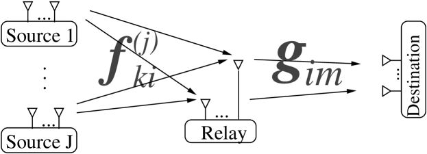
Figure 1: Multi-access relay networks.

Consider a relay network with $J$ sources each with $J_{a}$ antennas, one relay with $R_{a}$ antennas, and one destination with $M$ antennas. There is no direct connection from sources to the destination, because the sources are far from the destination. The system diagram is shown in Fig. 1.

Denote the fading coefficient from Antenna $k$ ($k=1,\ldots,J_{a}$) of Source $j$ ($j=1,\ldots,J$) to Antenna $i$ ($i=1,\ldots,R_{a}$) of the relay as $f^{(j)}_{ki}$. The $J_{a}\times 1$ channel vector from Source $j$ to relay Antenna $i$ is denoted as ${\bf f}_{i}^{(j)}$ whose $k$-th entry is $f^{(j)}_{ki}$. Denote the fading coefficient from relay Antenna $i$ to Antenna $m$ of the destination ($m=1,\ldots,M$) as $g_{im}$. The $R_{a}\times 1$ channel vector from the relay to destination Antenna $m$ is denoted as ${\bf g}_{m}$ whose $i$-th entry is $g_{im}$. All fading coefficients are assumed to be identically and independently distributed (i.i.d.) with $\mathcal{CN}(0,1)$ distribution. We assume a block-fading model with coherence interval $T$.

To allow IC at the relay, we assume that $R_{a}\geq J$. This can be realized through user admission control in the upper layers. We assume that sources have equal numbers of antennas. Our proposed protocol can be extended straightforwardly to networks where sources have unequal number of antennas. Further, to focus on the diversity performance, all sources and the relay are assumed to have the same average power constraint $P$. The extension to nonuniform power constraint is also straightforward. Throughout the paper, we assume global CSI at the destination; but the relay has only the backward CSI, i.e., channel information from sources to the relay. The channel information can be obtained by sending pilot sequences from sources and the relay [11, 18]. No feedback or channel estimation forwarding is required. Perfect synchronization at the symbol level is assumed for the network.

For complexity considerations, two linear constraints are imposed on the network. For one, the relay linearly transforms its received signal to generate its output signal without decoding. For the other, the decoding complexity at the destination is linear in the number of sources. It can be verified that the full-TDMA-DSTC scheme mentioned in the introduction section and the DSTC-ICRec scheme proposed in [13] satisfy these two linear constraints.

The general multi-user cooperative network has $J+N+1$ nodes. $J$ multi-antenna sources, denoted as $S=\left(s_{1},s_{2},\ldots,s_{J}\right)$, send independent information to $N$ multi-antenna destinations, denoted as $D=\left(d_{1},d_{2},\ldots,d_{N}\right)$, through one $R_{a}$-antenna relay. In an indoor environment, the mobile stations can be the sources and the destinations, and the access points connecting through cables can be the relay. The set of sources from which Destination $n$ receives information is described as $I_{n}=\{s,s\in S\}$. The profile of communication flows of the whole network can be described as $I=\left(I_{1},I_{2},\ldots,I_{N}\right)$. For example, a network with three single-antenna sources $S=\left(s_{1},s_{2},s_{3}\right)$, two single-antenna destinations $D=\left(d_{1},d_{2}\right)$, and one four-antenna relay is shown in Fig. 2. Destination 1 receives information from Sources 1 and 2, while Destination 2 receives information from Sources 2 and 3. The profile of communication flows can be expressed as $I=\left(\{s_{1},s_{2}\},\{s_{2},s_{3}\}\right)$. Specifically, when $J=N$ and $I=\left(\{s_{1}\},\{s_{2}\},\cdots,\{s_{N}\}\right)$, the network becomes the interference relay network with parallel communication flows. When $N=1$ and $I=\left(\{s_{1},\cdots,s_{J}\}\right)$, the network becomes the MARN. All nodes are assumed to be synchronized. Extension to asynchronous networks is straightforward using the random access and IC methods in [19]. Although for the clarity of presentation, we present our protocol using the MARN model, we will show that it can be applied straightforwardly to this general network model.

III IC at the Relay: IC-Relay-TDMA

It is well known that for cooperative networks relaying can improve communication reliability and coverage. In this paper, we show a new dimension in the design of multi-user relay networks: IC at relays. In our MARNs, to improve the spectral efficiency, we allow concurrent multi-user transmission in the link between the source and the relay. Since this source-relay link is a multi-antenna multi-access channel (MAC), the multi-antenna relay has the potential to cancel the induced multi-user interference. Cancelling interference at the relay improves the signal to interference-plus-noise ratio of the relay-destination link and simplify the signal processing at the destination. Thus, this idea has the potential of providing good performance when the relay-destination link is the bottleneck of the network. Based on the above considerations, we propose a protocol called IC-Relay-TDMA, in which the relay conducts IC using linear transformations but not decoding before forwarding int-free signal to the destination by TDMA. In Subsection III-A, we describe the protocol for general $(J,J_{a},R_{a},M)$ MARNs. Its application in a general multi-user cooperative network is discussed in Subsection III-B. Then, the use of IC-Relay-TDMA in one simple network is illustrated in Subsection III-C as an example.

III-A The Protocol of IC-Relay-TDMA

In this subsection, we explain the protocol of IC-Relay-TDMA. The protocol consists of two phases. During the first phase, all sources send information to the relay simultaneously using STBC with ABBA structure[20, 21]. The relay overhears superimposed signals of all source information and conducts multi-user IC[16]. During the second phase, the relay conducts a scheme called MRC-STBC to enhance the communication reliability in the second transmission, then forwards information of different sources in TDMA to the destination. The destination decodes each source’s information independently. A block diagram of IC-Relay-TDMA is shown in Fig. 3. The details of the protocol and corresponding formulas are described in the following. First, we consider the scenarios when $J_{a}$ is a power-of-2, then extend to the cases that $J_{a}$ is not a power-of-2.

Phase 1

When the number of antennas at each source is a power-of-2, i.e., $J_{a}=2^{n},n\in\mathcal{N}$, each transmitter constructs $\frac{J_{a}}{2}$ constellations (e.g. PSK, QAM constellation and their rotations), denoted as $\mathcal{S}_{u},u=1,\ldots,\frac{J_{a}}{2}$. The average power of the constellations is normalized to be one. The constellations need to satisfy the following condition for diversity gain:

$$\underset{u=1:\frac{J_{a}}{2}}{\sum}c_{u}s_{u}\neq 0,\ \forall s_{u}\in\mathcal{S}_{u},c_{u}\in\{-1,0,1\}.$$ (1)

One approach to construct such constellations is through rotation[22, 23]. For example, when $J_{a}=4$, i.e., $n=2$, two BPSK constellations can be constructed as $\mathcal{S}_{1}=\{-1,1\}$ and $\mathcal{S}_{2}=\{\mathrm{j},-\mathrm{j}\}$, where $\mathcal{S}_{2}$ is rotated from $\mathcal{S}_{1}$ by $\pi/2$. It can be verified that $\mathcal{S}_{1}$ and $\mathcal{S}_{2}$ satisfy the condition in (1).

Source $j$ independently and uniformly collects $J_{a}$ symbols $s_{k}^{(j)},k=1,\ldots,J_{a}$ from these $J_{a}/2$ constellations with $s_{2u-1}^{(j)},s_{2u}^{(j)}\in\mathcal{S}_{u}$. Then, a $J_{a}\times J_{a}$ STBC with ABBA structure [21, 20] is constructed by

$$\mathbf{S}^{(j)}=\mathbf{S}_{n}\left(s^{(j)}_{1},s^{(j)}_{2},\ldots,s^{(j)}_{J_{a}}\right),$$

where the function $\mathbf{S}_{n}$ maps $J_{a}$ variables to a $J_{a}\times J_{a}$ matrix through an iterative procedure as

$$\mathbf{S}_{n}\left(s_{1},s_{2},\ldots,s_{J_{a}}\right)=\left[\begin{array}[]{cc}\mathbf{S}_{n-1}\left(s_{1},\ldots,s_{\frac{J_{a}}{2}}\right)&\mathbf{S}_{n-1}\left(s_{\frac{J_{a}}{2}+1},\ldots,s_{J_{a}}\right)\\ \mathbf{S}_{n-1}\left(s_{\frac{J_{a}}{2}+1},\ldots,s_{J_{a}}\right)&\mathbf{S}_{n-1}\left(s_{1},\ldots,s_{\frac{J_{a}}{2}}\right)\end{array}\right],$$

with $\mathbf{S}_{1}(s_{1},s_{2})$ an $2\times 2$ Alamouti code. All sources transmit simultaneously in this phase. The length of this phase is $T_{1}=J_{a}$ time slots. It is thus assumed that the coherence interval $T$ is no less than $J_{a}$.

Relay Antenna $i$ overhears a $T_{1}\times 1$ signal vector as

$${\bf r}_{i}=\sum_{j=1}^{J}\sqrt{\frac{P}{J_{a}}}{\mathbf{S}}^{(j)}{\bf f}_{i}^{(j)}+{\bf v}_{i},$$ (2)

where $\mathbf{v}_{i}$ denotes the $J_{a}\times 1$ additive white Gaussian noise (AWGN) vector, whose $\tau$-th entry $v_{\tau i}$ is i.i.d. $\mathcal{CN}(0,1)$ distributed. Note that the first phase transmission is virtually a multi-antenna multi-access channel. When $R_{a}\geq J$, the IC scheme originally proposed for direction transmission [16] can be conducted at the relay to fully cancel the multi-user interference. In [16], the IC procedure was discussed explicitly only for a system with at most four antennas at each source. Here, we describe this procedure for a general system with $J_{a}=2^{n}$ antennas at each source. Without loss of generality, we discuss how the relay cancels interference from Source 2 to Source $J$ and obtains an int-free observation of the information of Source 1.

The IC procedure has two steps. In the first step, the relay separates the system that communicates $J_{a}=2^{n}$ symbols for each source into $2^{n-1}$ equivalent Alamouti systems. In the second step, the IC scheme in [15] is applied to each Alamouti system to iteratively cancel interference from Source 2 to Source $J$. Denote $\mathbf{h}_{l}$ as the $l$-th row of the $2^{n-1}\times 2^{n-1}$ Hadamard matrix $\mathbf{H}_{n-1}$. Let $\mathbf{s}^{(j)}_{\mathrm{o}}=\left[s^{(j)}_{1},s^{(j)}_{3},\ldots,s^{(j)}_{2^{n}-1}\right]^{t},\mathbf{s}^{(j)}_{\mathrm{e}}=\left[s^{(j)}_{2},s^{(j)}_{4},\ldots,s^{(j)}_{2^{n}}\right]^{t},{\mathbf{f}}^{(j)}_{i\mathrm{o}}=\left[f^{(j)}_{1i},f^{(j)}_{3i},\ldots,f^{(j)}_{(2^{n}-1)i}\right]^{t},{\mathbf{f}}^{(j)}_{i\mathrm{e}}=\left[f^{(j)}_{2i},f^{(j)}_{4i},\ldots,f^{(j)}_{2^{n}i}\right]^{t},\mathbf{v}_{i\mathrm{o}}=\left[v_{1i},v_{3i},\ldots,v_{(2^{n}-1)i}\right]^{t}$, and $\mathbf{v}_{i\mathrm{e}}=\left[v_{2i},v_{4i},\ldots,v_{(2^{n})i}\right]^{t}$. As the first step, relay Antenna $i$ calculates $\tilde{\mathbf{r}}_{li}=(\mathbf{h}_{l}\otimes\mathbf{I}_{2})\mathbf{r}_{i}$ to obtain equivalent Alamouti systems as follows,

$$\tilde{\mathbf{r}}_{li}=(\mathbf{h}_{l}\otimes\mathbf{I}_{2})\mathbf{r}_{i}=\sum_{j=1:J}\sqrt{\frac{P}{J_{a}}}\mathbf{S}_{1}\left(\mathbf{h}_{l}\mathbf{s}^{(j)}_{\mathrm{o}},\mathbf{h}_{l}\mathbf{s}^{(j)}_{\mathrm{e}}\right)\left[\begin{array}[]{c}\mathbf{h}_{l}{\mathbf{f}}^{(j)}_{i\mathrm{o}}\\ \mathbf{h}_{l}{\mathbf{f}}^{(j)}_{i\mathrm{e}}\end{array}\right]+\left[\begin{array}[]{c}\mathbf{h}_{l}\mathbf{v}_{i\mathrm{o}}\\ \mathbf{h}_{l}\mathbf{v}_{i\mathrm{e}}\end{array}\right],\ l=1,\ldots,2^{n-1}.$$ (3)

Denote the first and second entries of $\tilde{\mathbf{r}}_{li}$ as $\tilde{r}_{li1}$ and $\tilde{r}_{li2}$, respectively. Due to the Alamouti structure of $\mathbf{S}_{1}\left(\mathbf{h}_{l}\mathbf{s}^{(j)}_{\mathrm{o}},\mathbf{h}_{l}\mathbf{s}^{(j)}_{\mathrm{e}}\right)$. Eq. (3) can be equivalently rewritten as

$$\underset{\hat{\mathbf{r}}_{li}}{\underbrace{\left[\begin{array}[]{c}\tilde{r}_{li1}\\ -\overline{\tilde{r}_{li2}}\end{array}\right]}}=\sum_{j=1:J}\sqrt{\frac{P}{J_{a}}}\underset{\mathbf{F}^{(j)}_{li}}{\underbrace{\mathbf{S}_{1}\left(\mathbf{h}_{l}{\mathbf{f}}^{(j)}_{i\mathrm{o}},\mathbf{h}_{l}{\mathbf{f}}^{(j)}_{i\mathrm{e}}\right)}}\underset{\hat{\mathbf{s}}_{l}^{(j)}}{\underbrace{\left[\begin{array}[]{c}\mathbf{h}_{l}\mathbf{s}^{(j)}_{\mathrm{o}}\\ \mathbf{h}_{l}\mathbf{s}^{(j)}_{\mathrm{e}}\end{array}\right]}}+\underset{\hat{\mathbf{v}}_{li}}{\underbrace{\left[\begin{array}[]{c}\mathbf{h}_{l}\mathbf{v}_{i\mathrm{o}}\\ -\overline{\mathbf{h}_{l}\mathbf{v}_{i\mathrm{e}}}\end{array}\right]}}.$$ (4)

For the second step, the relay cancels interference for each Alamouti system in multiple iterations, where interference of one source is cancelled in each iteration. Stack $\hat{\mathbf{r}}_{li}$ and $\mathbf{F}_{li}^{(j)}$ at different relay antenna as $\hat{\mathbf{r}}_{l}=[\hat{\mathbf{r}}_{l1}^{t},\cdots,\hat{\mathbf{r}}_{lR_{a}}^{t}]^{t}$ and $\mathbf{F}^{(j)}_{l}=\left[\mathbf{F}_{l1}^{(j)t},\cdots,\mathbf{F}_{lR_{a}}^{(j)t}\right]^{t}$. Denote $\mathcal{F}_{l}(i)$ as the $2(R_{a}-i-1)\times 2(R_{a}-i)$ IC matrix to cancel Source $J-i$ for System $l$; $\mathbf{r}_{l}(i)$ and $\mathbf{F}_{l}(i)$ as the remaining $2(R_{a}-i)\times 1$ signal vector and the remaining $2(R_{a}-i)\times 2J$ equivalent channel matrix after cancelling Source $J-i+1$ for System $l$, respectively. The iterative IC procedures are as follows:

• Initialization: $\mathbf{F}_{l}(0)=[\mathbf{F}_{l}^{(1)},\ldots,\mathbf{F}_{l}^{(J)}]$, $\mathbf{r}_{l}(0)=\hat{\mathbf{r}}_{l}$.

• Iteration: For $i=0$ to $J-2$,

  1. Form the IC matrix $\mathcal{F}_{l}(i)$ as
     

     $${\mathcal{F}_{l}(i)}=\left[\begin{array}[]{ccccc}-\frac{2{\mathbf{F}}_{l,J-i,1}^{(i)*}}{\|{\mathbf{F}}_{l,J-i,1}^{(i)}\|^{2}}&\frac{2{\mathbf{F}}_{l,J-i,2}^{(i)*}}{\|{\mathbf{F}}_{l,J-i,2}^{(i)}\|^{2}}&\mathbf{0}_{2}&\ldots&\mathbf{0}_{2}\\ -\frac{2{\mathbf{F}}_{l,J-i,1}^{(i)*}}{\|{\mathbf{F}}_{l,J-i,1}^{(i)}\|^{2}}&\mathbf{0}_{2}&\frac{2{\mathbf{F}}_{l,J-i,3}^{(i)*}}{\|{\mathbf{F}}_{l,J-i,3}^{(i)}\|^{2}}&\ldots&\mathbf{0}_{2}\\ \vdots&\vdots&\vdots&\ddots&\vdots\\ -\frac{2{\mathbf{F}}_{l,J-i,1}^{(i)*}}{\|{\mathbf{F}}_{l,J-i,1}^{(i)}\|^{2}}&\mathbf{0}_{2}&\mathbf{0}_{2}&\ldots&\frac{2{\mathbf{F}}_{l,J-i,M-i}^{(i)*}}{\|{\mathbf{F}}_{l,J-i,M-i}^{(i)}\|^{2}}\end{array}\right]_{2(R_{a}-i-1)\times 2(R_{a}-i)}$$ (9)

  2. Cancel interference of Source $J-i$ by multiplying $\mathbf{r}_{l}(i)$ with $\mathcal{F}_{l}(i)$. The remained equivalent received signal can be calculated as $\mathbf{r}_{l}(i+1)=\mathcal{F}_{l}(i)\mathbf{r}_{l}(i)$ and the remained equivalent channel matrix can be calculated as $\mathbf{F}_{l}(i+1)=\mathcal{F}_{l}(i)\mathbf{F}_{l}(i)$.

The $2\times 2$ matrix $\mathbf{F}_{l,p,q}^{(i)}$ in (9) denotes the $(p,q)$th $2\times 2$ submatrix of $\mathbf{F}_{l}(i)$. After $J-1$ iterations, information of Sources $J$ to 2 is cancelled and the remaining signal vector $\mathbf{r}_{l}(J-1)$ only contains information of Source 1. The overall IC matrix that jointly cancels Sources 2 to $J$ is $\mathcal{F}_{l}\triangleq\prod_{i=0}^{J-2}\mathcal{F}_{l}(i)$. To help the presentation, let $\hat{\mathbf{r}}_{l}^{(1)}=\mathbf{r}_{l}(J-1)$. From this iterative procedure, we have

$$\hat{\mathbf{r}}_{l}^{(1)}=\mathcal{F}_{l}\hat{\mathbf{r}}_{l}=\sqrt{\frac{P}{J_{a}}}\mathcal{F}_{l}\mathbf{F}_{l}^{(1)}\hat{\mathbf{s}}_{l}^{(1)}+\mathcal{F}_{l}\mathbf{v}_{l},$$ (10)

where $\mathbf{v}_{l}=[\hat{\mathbf{v}}_{l1}^{t},\hat{\mathbf{v}}_{l2}^{t},\cdots,\hat{\mathbf{v}}_{lR_{a}}^{t}]^{t}$. A $2(R_{a}-J+1)\times 1$ vector observation of Source 1’s information is carried in $\hat{\mathbf{r}}_{l}^{(1)}$. Eq. (10) implies that the rows of $\mathcal{F}_{l}$ are in the null spaces of the columns of $\mathbf{F}_{l}^{(2)}$ to $\mathbf{F}_{l}^{(J)}$, i.e., $\mathcal{F}_{l}\mathbf{F}_{l}^{(j)}=\mathbf{0}$ for $j=2,\ldots,J$. Thus, this IC process is an iterative realization of ZF. Different from conventional ZF which uses pseudo-inverse of the channel matrix, the IC method needs no channel matrix inversion. Similarly, the relay can obtain int-free vector observations of other sources’ information.

Phase 2

In this phase, the relay conducts a process called MRC-STBC[24], then forwards information of each source to the destination in different time slots. The destination decodes source-by-source and jointly recovers the symbols contained in $\mathbf{s}_{\mathrm{o}}^{(j)}$. Without loss of generality, we only consider how Source 1’s information is processed by the relay and decoded at the destination. The maximum-ratio combining (MRC) step is first conducted to maximize the SNR of $\hat{\mathbf{r}}_{l}^{(1)}$. The MRC can be represented as

$$\tilde{\mathbf{s}}_{l}^{(1)}=\frac{2\mathbf{F}_{l}^{(1)*}\mathcal{F}_{l}^{*}(\mathcal{F}_{l}\mathcal{F}_{l}^{*})^{-1}\hat{\mathbf{r}}_{l}^{(1)}}{{\rm tr}\,(\mathbf{F}_{l}^{(1)*}\mathcal{F}_{l}^{*}(\mathcal{F}_{l}\mathcal{F}_{l}^{*})^{-1}\mathcal{F}_{l}\mathbf{F}_{l}^{(1)})}=\sqrt{\frac{P}{J_{a}}}\hat{\mathbf{s}}_{l}^{(1)}+\underset{\tilde{\mathbf{v}}_{l}^{(1)}}{\underbrace{\frac{2\mathbf{F}_{l}^{(1)*}\mathcal{F}_{l}^{*}(\mathcal{F}_{l}\mathcal{F}_{l}^{*})^{-1}\mathcal{F}_{l}\mathbf{v}_{l}}{{\rm tr}\,(\mathbf{F}_{l}^{(1)*}\mathcal{F}_{l}^{*}(\mathcal{F}_{l}\mathcal{F}_{l}^{*})^{-1}\mathcal{F}_{l}\mathbf{F}_{l}^{(1)})}}}.$$ (11)

The entries of $\tilde{\mathbf{s}}_{l}^{(1)}$, the vector after MRC, are soft estimates of the entries of $\hat{\mathbf{s}}_{l}^{(1)}$. From (3), (4), (10), and (11), the covariance matrix of $\tilde{\mathbf{v}}_{l}^{(1)}$ can be calculated as $\frac{J_{a}}{{\rm tr}\,\{\mathbf{F}_{l}^{(1)*}\mathcal{F}_{l}^{*}(\mathcal{F}_{l}\mathcal{F}_{l}^{*})^{-1}\mathcal{F}_{l}\mathbf{F}_{l}^{(1)}\}}\mathbf{I}_{2}$, which implies that the two noise elements in $\tilde{\mathbf{v}}_{l}^{(1)}$ are i.i.d.. Also, the noise vectors $\tilde{\mathbf{v}}_{l}^{(1)}$ of different Alamouti systems are independent, due to the orthogonality of the Hadamard matrix $\mathbf{H}_{n-1}$, but not identical. Following the MRC step, to forward Source 1’s information, the relay uses generalized orthogonal STBCs to encode entries of $\tilde{\mathbf{s}}_{l}^{(1)}$. We especially consider generalized orthogonal STBCs because of its full diversity and symbol-wise decoding [25]. Other designs such as quasi-orthogonal STBCs [21] can also be applied but with higher decoding complexity. In general, consider using a $T_{2}\times R_{a}$ generalized complex orthogonal design that carries $K$ symbols. Note that each $\tilde{\mathbf{s}}_{l}^{(1)}$ contains information of two symbols. The relay waits for $K$ symbols from $\lceil K/2\rceil$ Alamouti systems, denoted as $\tilde{s}_{k}^{(1)},k=1,\ldots,K$ (the subscript $l$ is removed without confusion for conciseness), to generate the $T_{2}\times R_{a}$ codeword as

$$\left[\begin{array}[]{ccc}\mathbf{t}_{1}&\cdots&\mathbf{t}_{R_{a}}\end{array}\right]=c\sum_{k=1:K}\left({\rm Re}\,\{\tilde{s}_{k}^{(1)}\}\mathbf{A}_{k}+\mathrm{j}{\rm Im}\,\{\tilde{s}_{k}^{(1)}\}\mathbf{B}_{k}\right),$$ (12)

where $\mathbf{t}_{i}$ is the $T_{2}\times 1$ signal vector to be transmitted at relay Antenna $i$; $\mathbf{A}_{k}$ and $\mathbf{B}_{k}$ are $T_{2}\times R_{a}$ relay encoding matrices for generalized orthogonal designs as found in (4.67) in [26]; and $c\triangleq\sqrt{\frac{PT_{2}}{R_{a}K(\frac{P}{2}+\frac{1}{2R_{a}-2J+1})}}$ is the power normalization coefficient at the relay. Since the processing in (3), (10), (11), and (12) are linear, the transmitted signal vectors at the relay are linear in its received signal vectors $\mathbf{r}_{i}$. Assume that the coherence interval $T$ is no less than $T_{2}$. The relay concurrently forwards $\mathbf{t}_{i}$ on Antenna $i$. The received $T_{2}\times 1$ signal vector at destination Antenna $m$ can be expressed as

$$\mathbf{x}_{m}=\sum_{i=1:R_{a}}\mathbf{t}_{i}g_{im}+\mathbf{w}_{m}=c\sqrt{\frac{P}{J_{a}}}\sum_{k=1:K}\left({\rm Re}\,\{\tilde{s}_{k}^{(1)}\}\mathbf{A}_{k}+\mathrm{j}{\rm Im}\,\{\tilde{s}_{k}^{(1)}\}\mathbf{B}_{k}\right){\mathbf{g}}_{m}+{\mathbf{u}_{m}},$$ (13)

where $\mathbf{w}_{m}$ denotes the $T_{2}\times 1$ AWGN vector at destination Antenna $m$; $\mathbf{u}_{m}$ denotes the equivalent noise vector, $\mathbf{u}_{m}=c\underset{{k=1:K}}{\sum}\left({\rm Re}\,\{\tilde{v}_{k}^{(1)}\}\mathbf{A}_{k}+\mathrm{j}{\rm Im}\,\{\tilde{v}_{k}^{(1)}\}\mathbf{B}_{k}\right)\hat{\mathbf{g}}_{m}+{\mathbf{w}_{m}}$ with $\tilde{v}_{k}^{(1)}$ the additive noise defined in (11).

At the destination, a $2T_{2}M\times 1$ vector is formed by stacking $\mathbf{x}_{m}$ into $\tilde{\mathbf{x}}=\left[{\rm Re}\,\{\mathbf{x}_{1}\}^{t},{\rm Im}\,\{\mathbf{x}_{1}\}^{t},\cdots,\right.$ $\left.{\rm Re}\,\{\mathbf{x}_{M}\}^{t},{\rm Im}\,\{\mathbf{x}_{M}\}^{t}\right]^{t}$. After straightforward calculation, the system equation can be written as

$$\tilde{\mathbf{x}}=c\sqrt{\frac{P}{J_{a}}}\underset{\tilde{\mathbf{G}}}{\underbrace{\left[\begin{array}[]{ccccc}\mathcal{A}_{1}\tilde{\mathbf{g}}_{1}&\mathcal{B}_{1}\tilde{\mathbf{g}}_{1}&\cdots&\mathcal{A}_{K}\tilde{\mathbf{g}}_{1}&\mathcal{B}_{K}\tilde{\mathbf{g}}_{1}\\ \vdots&\vdots&\ddots&\vdots&\vdots\\ \mathcal{A}_{1}\tilde{\mathbf{g}}_{M}&\mathcal{B}_{1}\tilde{\mathbf{g}}_{M}&\cdots&\mathcal{A}_{K}\tilde{\mathbf{g}}_{M}&\mathcal{B}_{K}\tilde{\mathbf{g}}_{M}\end{array}\right]}}\left[\begin{array}[]{c}{\rm Re}\,\tilde{s}_{1}^{(1)}\\ {\rm Im}\,\tilde{s}_{1}^{(1)}\\ \vdots\\ {\rm Re}\,\tilde{s}_{K}^{(1)}\\ {\rm Im}\,\tilde{s}_{K}^{(1)}\end{array}\right]+\underset{\hat{\mathbf{u}}}{\underbrace{c\tilde{\mathbf{G}}\left[\begin{array}[]{c}{\rm Re}\,\tilde{v}_{1}^{(1)}\\ {\rm Im}\,\tilde{v}_{1}^{(1)}\\ \vdots\\ {\rm Re}\,\tilde{v}_{K}^{(1)}\\ {\rm Im}\,\tilde{v}_{K}^{(1)}\end{array}\right]+\left[\begin{array}[]{c}{\rm Re}\,{\mathbf{w}_{1}}\\ {\rm Im}\,{\mathbf{w}_{1}}\\ \vdots\\ {\rm Re}\,{\mathbf{w}_{M}}\\ {\rm Im}\,{\mathbf{w}_{M}}\end{array}\right]}},$$ (14)

where

$$\tilde{\mathbf{g}}_{m}=\left[\begin{array}[]{c}{\rm Re}\,\{{\mathbf{g}}_{m}\}\\ {\rm Im}\,\{{\mathbf{g}}_{m}\}\end{array}\right],\ \mathcal{A}_{k}=\left[\begin{array}[]{cc}{\rm Re}\,\{\mathbf{A}_{k}\}&-{\rm Im}\,\{\mathbf{A}_{k}\}\\ {\rm Im}\,\{\mathbf{A}_{k}\}&{\rm Re}\,\{\mathbf{A}_{k}\}\end{array}\right],\hskip 2.84526pt\mathcal{B}_{k}=\left[\begin{array}[]{cc}-{\rm Im}\,\{\mathbf{B}_{k}\}&-{\rm Re}\,\{\mathbf{B}_{k}\}\\ {\rm Re}\,\{\mathbf{B}_{k}\}&-{\rm Im}\,\{\mathbf{B}_{k}\}\end{array}\right].$$

With generalized complex orthogonal designs, $\tilde{\mathbf{G}}^{t}\tilde{\mathbf{G}}=\|\mathbf{G}\|^{2}\mathbf{I}_{2K}$, where $\mathbf{G}=[\mathbf{g}_{1},\ldots,\mathbf{g}_{M}]$. Denote $\mathbf{a}_{k}$ as a $1\times 2K$ vector whose $2k-1$ and $2k$ entries are $1$ and $\mathrm{j}$, respectively, and all the other entries are zero. The destination can obtain a soft estimate of $\tilde{s}_{k}^{(1)}$ by the following calculation,

$$x_{k}=\mathbf{a}_{k}\frac{\tilde{\mathbf{G}}^{t}\tilde{\mathbf{x}}}{\|\mathbf{G}\|^{2}}=c\sqrt{\frac{P}{J_{a}}}\tilde{s}_{k}^{(1)}+c\tilde{v}_{k}^{(1)}+\frac{w_{k}}{\|\mathbf{G}\|},$$ (16)

where $w_{k}$ is the equivalent noise with $\mathcal{CN}(0,1)$ distribution and independent for different $k$. $x_{k}$ is a soft estimate to $\tilde{s}_{k}^{(1)}$, which is a linear superposition of Source 1’s symbols from (4). Without loss of generality, we assume that $\tilde{s}_{k}^{(1)}$ provides a soft estimate to $\mathbf{h}_{k}\mathbf{s}^{(1)}_{\mathrm{o}},k=1,\ldots,2^{n-1}$. Denote $\mathbf{x}=\left[\begin{array}[]{ccc}x_{1}&\ldots&x_{2^{n-1}}\end{array}\right]^{t},\tilde{\mathbf{v}}^{(1)}=\left[\begin{array}[]{ccc}\tilde{v}_{1}^{(1)}&\ldots&\tilde{v}_{2^{n-1}}^{(1)}\end{array}\right]^{t}$ and $\mathbf{w}=\left[\begin{array}[]{ccc}w_{1}&\ldots&w_{2^{n-1}}\end{array}\right]^{t}$. From (16), we have

$$\mathbf{x}=c\sqrt{\frac{P}{J_{a}}}\mathbf{H}_{n-1}\mathbf{s}^{(1)}_{\mathrm{o}}+\underset{{\mathbf{u}}}{\underbrace{c\tilde{\mathbf{v}}^{(1)}+\frac{\mathbf{w}}{\|\mathbf{G}\|}}}.$$ (17)

The destination performs ML decoding to decode $\mathbf{s}^{(1)}_{\mathrm{o}}$ based on (17) as

$$\arg\min_{\mathbf{s}}\left(\mathbf{x}-c\sqrt{\frac{P}{J_{a}}}\mathbf{H}_{n-1}\mathbf{s}\right)^{*}\mathbf{\Sigma}^{-1}_{\mathbf{u}}\left(\mathbf{x}-c\sqrt{\frac{P}{J_{a}}}\mathbf{H}_{n-1}\mathbf{s}\right),$$ (18)

where $\mathbf{\Sigma}_{\mathbf{u}}$ is the covariance matrix of the equivalent noise vector $\mathbf{u}$. After straightforward calculation, we have

$$\mathbf{\Sigma}_{\mathbf{u}}=2^{n-1}c^{2}{\rm diag}\,\left(\frac{1}{\gamma_{1}},\frac{1}{\gamma_{2}},\ldots,\frac{1}{\gamma_{2^{n-1}}}\right)+\frac{1}{\gamma_{g}}\mathbf{I}_{2^{n-1}},$$ (19)

where $\gamma_{l}=\frac{1}{2}{\rm tr}\,\{\mathbf{F}_{l}^{(1)*}\mathcal{F}_{l}^{*}(\mathcal{F}_{l}\mathcal{F}_{l}^{*})^{-1}\mathcal{F}_{l}\mathbf{F}_{l}^{(1)}\}$ and $\gamma_{g}=\|\mathbf{G}\|^{2}$. Similarly, $\mathbf{s}_{\mathrm{e}}^{(1)}$ can be jointly decoded. Transmission of other sources’ symbols can be performed similarly using orthogonal time slots. To decode all symbols from all $J$ sources, the destination only needs to conduct $2J$ procedures of ML decoding of $2^{n-1}$ symbols. The complexity is linear in the number of sources.

When $J_{a}$ is not a power-of-2, $2^{n}\times 2^{n}$ quasi-orthogonal STBCs with ABBA structure are used with $2^{n}$ the smallest power-of-2 number greater than $J_{a}$. During the first phase, each source concurrently transmits the first $J_{a}$ columns of the block codes in $T_{1}=2^{n}$ time slots. Similar to the case when $J_{a}$ is a power-of-2, the resulting multi-user interference can be cancelled using Eq. (3), (4), and (10) at the relay by treating $f^{(j)}_{ki}=0$ for $k=J_{a}+1,\ldots,2^{n}$. During the second step, symbols of different sources are forwarded by MRC-STBC in TDMA. Symbols are decoded source-by-source at the destination.

III-B Application in General Multi-User Cooperative Networks

IC-Relay-TDMA can be applied to the general multi-user cooperative networks with multiple destinations. During the first phase, all $J$ sources send information to the relay concurrently. The relay separates multi-user signals using IC without decoding. During the second phase, int-free soft estimates of each source’s symbols are encoded using STBC. The relay broadcasts each source’s block codes using TDMA. All destinations receive int-free signals from all sources. The destination decodes its desired information and discards undesired information. Note that transmission and processing at the relay do not depend on the relay-destination link and the number of destinations. IC-Relay-TDMA is robust to the dynamics of the destinations and no relay-destination channel information is required at the relay. On the contrary, for ZF relaying and MMSE relaying, the relay needs to acquire the channel information of new destinations and updates the scalar gain factors, which takes substantial protocol overhead. IC-Relay-TDMA can be applied to any patterns of communication flows when $R_{a}\geq J$, but ZF relaying and MMSE relaying require the flows to be parallel. It should be mentioned that IC-Relay-TDMA has a lower symbol rate than that of ZF and MMSE relaying. For the same bit rate, larger constellations are required.

III-C An Example: IC-Relay-TDMA for a $(2,2,2,1)$ MARN

In this subsection, we present one example of using IC-Relay-TDMA in a $(2,2,2,1)$ MARN, where there are two double-antenna sources, one double-antenna relay, and one single-antenna destination. The description of the proposed scheme in the previous subsection is lengthy as it is for a general MARN setting. In this network example, we will see that some processing are naturally simplified or become unnecessary and the main ideas behind the scheme are more clearly illustrated. The complexity at the relay and the destination can be further reduced.

During the first phase, only one constellation is required and the constraint on the constellation in (1) becomes trivial. Both sources collect two symbols from the same constellation, and concurrently send two Alamouti codes, i.e., $\mathbf{S}^{(j)}=\mathbf{S}_{1}\left(s_{1}^{(j)},s_{2}^{(j)}\right),\ j=1,2$. Since there is one Alamouti system only, the signal separation illustrated in (3) is also not needed. At the relay, only one round of IC iteration is needed. The interference of Source 2 can be cancelled by using the IC matrix $\mathcal{F}=\left[-\frac{2\mathbf{F}_{1}^{(2)*}}{\|\mathbf{F}_{1}^{(2)}\|^{2}},\frac{2\mathbf{F}_{2}^{(2)*}}{\|\mathbf{F}_{2}^{(2)}\|^{2}}\right]$, where $\mathbf{F}_{i}^{(j)}$ is the Alamouti channel matrix from Source $j$ to relay Antenna $i$, i.e., $\mathbf{F}_{i}^{(j)}=\mathbf{S}_{1}\left(f_{1i}^{(j)},f_{2i}^{(j)}\right)$. A $2\times 1$ vector observation of Source 1’s symbols can be obtained from (10). During the second phase, after the MRC represented in (11), the vector containing information of each source is encoded into an Alamouti block code and forwarded to the destination in TDMA. At the destination, the equivalent system equation for Source 1 can be written as

$$\underset{\hat{\mathbf{x}}}{\underbrace{\left[\begin{array}[]{c}x_{1}\\ -\overline{x_{2}}\end{array}\right]}}=c\sqrt{\frac{P}{2}}\mathbf{S}_{1}\left(g_{1},g_{2}\right)\underset{\mathbf{s}^{(1)}}{\underbrace{\left[\begin{array}[]{c}s_{1}^{(1)}\\ s_{2}^{(1)}\end{array}\right]}}+c\underset{\mathbf{u}}{\underbrace{\mathbf{S}_{1}\left(g_{1},g_{2}\right)\tilde{\mathbf{v}}^{(1)}+\tilde{\mathbf{w}}}},$$ (20)

where $x_{\tau}$, $\tilde{\mathbf{v}}^{(1)}$, and $\tilde{\mathbf{w}}$ denote the received signal at time slot $\tau$, the equivalent noise vector of the relay in (11), and the $2\times 1$ equivalent noise vector at the destination, respectively. The covariance matrices of $\tilde{\mathbf{v}}^{(1)}$ and $\tilde{\mathbf{w}}$ are $\gamma_{f}\mathbf{I}_{2}$ and $\mathbf{I}_{2}$, respectively, where $\gamma_{f}=\frac{1}{2}{\rm tr}\,\{\mathbf{F}^{(1)*}\mathcal{F}^{*}\left(\mathcal{F}\mathcal{F}^{*}\right)^{-1}\mathcal{F}\mathbf{F}^{(1)}\}$. Again, for this simple network, the processing in (14) is not needed. The destination directly performs the ML decoding based on (20), which, for this network, simplifies to

$$\arg\min_{\mathbf{s}^{(1)}}\left(\hat{\mathbf{x}}-c\sqrt{\frac{P}{2}}\mathbf{S}_{1}\left(g_{1},g_{2}\right)\mathbf{s}^{(1)}\right)^{*}\mathbf{\Sigma}_{\mathbf{u}}^{-1}\left(\hat{\mathbf{x}}-c\sqrt{\frac{P}{2}}\mathbf{S}_{1}\left(g_{1},g_{2}\right)\mathbf{s}^{(1)}\right),$$ (21)

where $\mathbf{\Sigma}_{\mathbf{u}}$ is the covariance matrix of the equivalent noise $\mathbf{u}$ and after straightforward calculation, $\mathbf{\Sigma}_{\mathbf{u}}=\left(c^{2}\gamma_{f}\left(\left|g_{1}\right|^{2}+\left|g_{2}\right|^{2}\right)+1\right)\mathbf{I}_{2}$. Since $\mathbf{\Sigma}_{\mathbf{u}}$ is a multiple of identity independent of the information symbol, it can be omitted in the ML decoding without any performance loss. Due to the Alamouti structure in $\mathbf{S}_{1}\left(g_{1},g_{2}\right)$, (21) can be further decomposed into two symbol-wise decodings.

IV Performance Analysis

In this section, we provide diversity analysis for the protocol of IC-Relay-TDMA and discuss its properties. Subsection IV-A is on the diversity analysis. In Subsection IV-B, we discuss the symbol rate of the scheme and when it achieves the int-free diversity.

IV-A Diversity Analysis

The diversity of a communication system is defined as the negative of the asymptotical slope of the bit error rate (BER), $d=-\underset{P\rightarrow\infty}{\lim}\frac{\log P_{b}}{\log P}.$ For fixed constellations, $P_{b}$ can be replaced with pairwise symbol error rate (SER). Since the ML decoding in (18) is source-by-source and the network parameters and processing at the relay and the destination are statistically homogenous, the diversity of each source is identical. We only need to analyze the diversity of one source, without loss of generality, Source 1. The concatenation of two hops of transmission and relay processing make the calculation of SER extremely difficult. Thus, to aid the diversity gain analysis, in the following lemma, we provide a method to calculate the diversity based on a formula with the outage probability structure without explicitly calculating the SER.

Lemma 1

Define the instantaneous normalized receive SNR as $\gamma={\rm tr}\,\{\mathbf{H}_{n-1}^{*}\mathbf{\Sigma}_{\mathbf{u}}^{-1}\mathbf{H}_{n-1}\}$. When the constellations satisfy (1), the diversity of the ML decoding in (18) can be calculated as

$$d=\lim_{\epsilon\rightarrow 0^{+}}\frac{\log P(\gamma<\epsilon)}{\log\epsilon}.$$ (22)

Proof:

See the appendix for the proof. ∎

Lemma 1 says that diversity can be calculated using the outage probability of the instantaneous normalized receive SNR. Thus, diversity can be obtained from the minimum exponent of $P(\gamma<\epsilon)$. More precisely, a random variable $\gamma$ provides diversity $d$ if $P(\gamma<\epsilon)=c\epsilon^{d}+o(\epsilon^{d})$ where $c$ is a constant independent of $\epsilon$. Before the diversity theorem, the following lemma is introduced.

Lemma 2

Let $\gamma_{1},\gamma_{2},\ldots,\gamma_{N},\gamma_{g}$ be $N+1$ instantaneous normalized receive SNRs. $\gamma_{g}$ is independent of $\gamma_{n}$ for $n=1,2,\ldots,N$. $\gamma_{g}$ provides diversity $d_{1}$; $\underset{n=1:N}{\sum}\gamma_{n}$ provides diversity $d_{2}$. If $\gamma=\underset{n=1:N}{\sum}\frac{\gamma_{n}\gamma_{g}}{\gamma_{n}+\gamma_{g}}$, $\gamma$ provides diversity $\min\{d_{1},d_{2}\}$.

Proof:

It can be shown by straightforward calculation that $\underset{n=1:N}{\sum}\frac{\gamma_{n}\gamma_{g}}{\gamma_{n}+\gamma_{g}}<\min\{\underset{n=1:N}{\sum}\gamma_{n},N\gamma_{1}\}$. The right-hand side has diversity $\min\{d_{2},d_{1}\}$ from Lemma 1. Therefore, the diversity of $\gamma$ is upperbounded by $\min\{d_{2},d_{1}\}$. To show the lowerbounds on the diversity, the following events are defined: $\mathcal{E}\triangleq\{\gamma_{1}<\gamma_{2}<\ldots<\gamma_{N}\}$, $\mathcal{E}_{n}\triangleq\mathcal{E}\bigcap\{\gamma_{n-1}<\gamma_{g}<\gamma_{n}\}$ for $n=1,\ldots,N+1$ where $\gamma_{0}=0$ and $\gamma_{N+1}=\infty$. Since $\{\mathcal{E}_{1},\mathcal{E}_{2},\ldots,\mathcal{E}_{N+1}\}$ is a partition of $\mathcal{E}$, we have

$$P(\gamma<\epsilon,\mathcal{E}) = P(\gamma<\epsilon,\mathcal{E}_{1})+P(\gamma<\epsilon,\mathcal{E}_{2})+\ldots+P(\gamma<\epsilon,\mathcal{E}_{N+1})$$

$$\leq \left(P(\gamma<\epsilon|\mathcal{E}_{1})+P(\gamma<\epsilon|\mathcal{E}_{2})+\ldots+P(\gamma<\epsilon|\mathcal{E}_{N+1})\right)\max\{P(\mathcal{E}_{n})\}$$

$$\leq \left(NP(\gamma_{g}<2\epsilon)+P\left(\underset{n=1:N}{\sum}\gamma_{n}<2\epsilon\right)\right)\max\{P(\mathcal{E}_{n})\}=c\epsilon^{d}+o(\epsilon^{d}),$$

where $d=\min\{d_{1},d_{2}\}$ and $c$ is a constant independent of $\epsilon$. For the third inequality, we have used the facts that $P\left(\gamma<\epsilon|\mathcal{E}_{n}\right)<P\left(\frac{\gamma_{g}\gamma_{N}}{\gamma_{g}+\gamma_{N}}<\epsilon|\mathcal{E}_{n}\right)<P(\gamma_{g}<2\epsilon)$ when $n\leq N$, and $P\left(\gamma<\epsilon|\mathcal{E}_{N+1}\right)<P\left(\underset{n=1:N}{\sum}\gamma_{n}<2\epsilon\right)$. In the third line, the term $\max\{P(\mathcal{E}_{n})\}$ is independent of $\epsilon$, hence does not affect the diversity. This is true for any orders of the sequence $\gamma_{1},\ldots,\gamma_{N}$. Note that $P(\gamma<\epsilon)=\underset{\mathcal{E}}{\sum}P(\gamma<\epsilon,\mathcal{E})$ where the summation is over all possible orders. The diversity of $\gamma$ is lowerbounded by the minimum of the exponents of $P(\gamma<\epsilon,\mathcal{E})$, which is $\min\{d_{2},d_{1}\}$. Therefore, the diversity is $\min\{d_{2},d_{1}\}$. ∎

Theorem 1

In $(J,J_{a},R_{a},M)$ MARNs, IC-Relay-TDMA achieves a diversity of $\min\{J_{a}(R_{a}-J+1),R_{a}M\}$ when $R_{a}\geq J$.

Proof:

From (18) and (19), the instantaneous normalized receive SNR can be calculated as

$$\gamma={\rm tr}\,\{\mathbf{H}_{n-1}^{*}\mathbf{\Sigma}_{\mathbf{u}}^{-1}\mathbf{H}_{n-1}\}=\underset{l=1:2^{n-1}}{\sum}\left(\frac{2^{n-1}c^{2}}{\gamma_{l}}+\frac{1}{\gamma_{g}}\right)^{-1}.$$ (23)

Since $\underset{l=1:2^{n-1}}{\sum}{\gamma_{l}}$ is identical to the instantaneous normalized receive SNR in a multi-antenna multi-user system with $J$ $J_{a}$-antenna users and IC at the $N$-antenna receiver, $\frac{1}{2^{n-1}c^{2}}\underset{l=1:2^{n-1}}{\sum}{\gamma_{l}}$ provides diversity $J_{a}(R_{a}-J+1)$[27]. Since $\gamma_{g}$ is a Gamma distributed random variable with degree $R_{a}M$, $\gamma_{g}$ provides diversity $R_{a}M$. By Lemma 2, $\gamma$ has diversity $\min\{J_{a}(R_{a}-J+1),R_{a}M\}$. ∎

IV-B Performance Discussions

This subsection discusses the condition for the proposed scheme to achieve the int-free diversity, the symbol rate, and the complexity of the proposed scheme. Comparisons with other schemes are also provided.

The int-free diversity condition

Theorem 1 says that IC-Relay-TDMA achieves diversity $\min\{J_{a}(R_{a}-J+1),R_{a}M\}$. Recall that the int-free diversity is defined as the maximum achievable diversity for $(J,J_{a},R_{a},M)$ MARNs without interference, which is $R_{a}\min\{J_{a},M\}$. When

$$M\leq J_{a}\left(1-\frac{J-1}{R_{a}}\right),$$ (24)

IC-Relay-TDMA achieves diversity $R_{a}M$, which is equal to the int-free diversity under (24). Eq. (24) is then called the int-free diversity condition. This condition implies that $M<J_{a}$, i.e., there are more independent paths in the source-relay link than the relay-destination link. For these networks, the bottleneck of transmission is the relay-destination link. Intuitively, when the source-relay link has extra degrees of freedom, they can be used for IC without degrading the total diversity. This is the basic idea behind IC-Relay-TDMA. Some examples of networks achieving the int-free diversity are $(2,2,2,1)$; $(2,4,2,1)$; and $(2,2,4,2)$ MARNs. To the best of our knowledge, in multi-antenna MAC, there is no IC method that achieves full single-user diversity. For MARNs, this is possible due to the extra relaying step. For networks satisfying (24), the source-relay link provides enough extra degrees of freedom to cancel interference at the relay.

The symbol rate

During the first phase, each source sends $T_{1}=2^{n}$ symbols during $T_{1}$ time slots. During the second phase, assume that the relay uses generalized orthogonal STBCs of dimension $T_{2}\times R_{a}$ to carry $K$ symbols. Then, the total number of time slots in the second phase is $\frac{JT_{1}T_{2}}{K}$. Let the symbol rate of the STBC code used in the second hop as $R_{o}\triangleq\frac{K}{T_{2}}$. Thus, the symbol rate of each source is $R=T_{1}/\left(T_{1}+\frac{JT_{1}T_{2}}{K}\right)=\frac{R_{o}}{J+R_{o}}$. If rate-1 codes (e.g., Alamouti code) are used in the second transmission phase, we have $R_{o}=1$ and the symbol rate of the scheme is $\frac{1}{1+J}$.

Complexity

We discuss the complexities in terms of the number of sources at the relay and the destination. Note that the relay needs to cancel the interfering signals from $J-1$ sources to obtain the int-free signal from one source and there are $J$ sources needed to be decoupled. The complexity of the IC is quadratic in the number of sources at the relay. At the destination, the complexity of ML decoding is linear in the number sources. Therefore, the relay has higher order of complexity than the destination in terms of the number of sources.

Comparison with other schemes

We now compare IC-Relay-TDMA with other schemes in MARNs. Recall that the proposed IC-Relay-TDMA scheme has concurrent transmission in the source-relay link only. We first compare it with full-TDMA-DSTC, which uses TDMA to avoid multi-user interference in both hops. The second compared scheme is DSTC-ICRec[13], which allows multi-user concurrent transmission in both hops and IC at the destination to decouple signals of different sources. Finally, we introduce DSTC joint-user ML decoding, which is similar to DSTC-ICRec excepts that, instead of conducting IC then decoding each source’s messages independently, the destination jointly decodes all sources’ messages. Note that the decoding complexity of this scheme is exponential in the number of sources. Thus, DSTC joint-user ML decoding does not satisfy the linear constraint at the destination mentioned in Section II, but the other three schemes satisfy the linear constraints both at the relay and the destination. We compare diversity, symbol rates, and other properties of these schemes in Table I. The details on the diversity results in this table can be found in [28].

For networks satisfying the int-free diversity condition, IC-Relay-TDMA achieves the same diversity as full-TDMA-DSTC with a higher transmission rate. This is due to the concurrent transmission and diversity redundancy in the source-relay link. Though the symbol rate of DSTC-ICRec is higher than that of IC-Relay-TDMA, a higher dimension constellation can be used for IC-Relay-TDMA to achieve the same bit rate with faster decaying error probability. DSTC joint-user ML decoding achieves the maximum int-free diversity with a symbol rate higher than that of IC-Relay-TDMA. However, the decoding complexity of the DSTC joint-user ML decoding is exponential in the number of sources, which is very demanding when $J$ is large. This implies that the proposed IC-Relay-TDMA trades decoding complexity for symbol rate without losing diversity for networks satisfying the int-free diversity condition. It should also be noted that IC-Relay-TDMA requires backward CSI at the relay, while the other three schemes do not require any CSI at the relay. Backward CSI can be obtained via training and does not need any feedback.

V Numerical Results

In this section, we show simulated BER performance of IC-Relay-TDMA and its comparison with other schemes. In all figures, the horizontal axis represents the average transmit SNR, measured in dB. Since the noises at all nodes are normalized, $P$ is equal to the average transmit SNR. The vertical axis represents the BER.

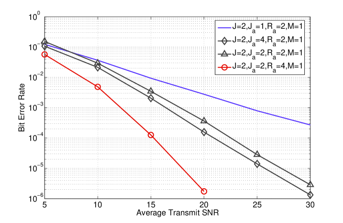
Figure 4: BER performance IC-Relay-TDMA, under BPSK modulation.

Fig. 4 is on the BERs of IC-Relay-TDMA under four network scenarios: Network 1: $(2,1,2,1)$ MARN; Network 2: $(2,2,2,1)$ MARN; Network 3: $(2,4,2,1)$ MARN; and Network 4: $(2,2,4,1)$ MARN. For the first three networks, Alamouti codes are used; and for Network 4, the rate $3/4$ generalized orthogonal STBC shown in (4.103) of [26] is used. All networks apply BPSK modulation. Networks 2, 3, and 4 satisfy the int-free diversity. Fig. 4 shows that for these three networks, the proposed scheme achieves the int-free diversity 2 for Networks 2 and 3; and 4 for Network 4. Network 1 does not satisfy the int-free condition in (24). Fig. 4 shows that Network 1 has diversity 1, which is less than 2, the int-free diversity. These simulation results verify Theorem 1.

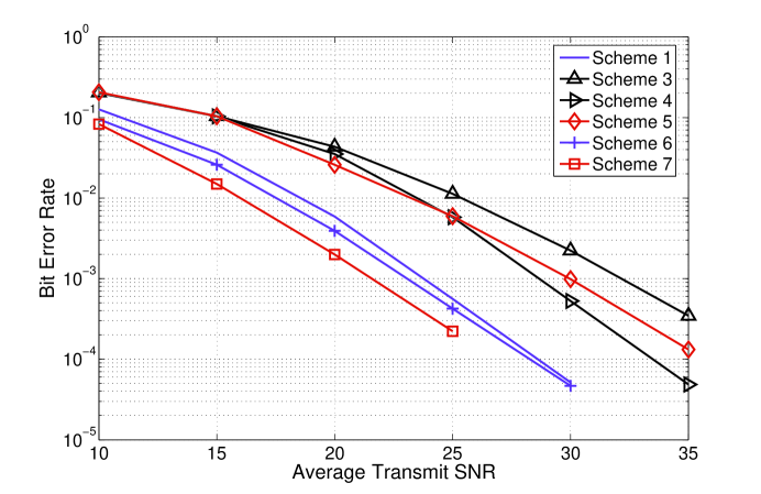
Figure 6: Performance comparison in a $(2,2,2,1)$ MARN, under 1 bit/user/channel use.

In what follows, we compare the proposed IC-Relay-TDMA (Scheme 1) with DSTC-ICRec (Scheme 2), full-TDMA-DSTC (Scheme 3), full-TDMA-DSTC CIR (Scheme 4), DSTC joint-user ML decoding (Scheme 5), IC-Relay-TDMA DF (Scheme 6), joint-DF-TDMA (Scheme 7) in the $(2,1,2,2)$ and $(2,2,2,1)$ MARNs. Schemes 1, 2, 3, and 5 are discussed in Subsection IV-B. To rule out the effect of the difference in the CSI requirements for Scheme 1 (the relay needs to know its channels with the transmitters) and Scheme 3 (no channel information at the relay), Scheme 4, originally proposed in [29] for single-user relay networks, is included as well. In this scheme, the relay uses its knowledge of the backward CSI to equalize the phase shift of the source-relay link, then forwards information to the destination by Alamouti DSTC. To allow decoding at the relay, Scheme 6 is introduced, which is similar to Scheme 1 except that all sources’ symbols are decoded after IC at the relay and re-modulated by the same constellation before forwarding. For Scheme 7, the relay jointly decodes symbols from both sources without IC before forwarding each source’s information using Alamouti DSTC in TDMA. Note that Schemes 1, 2, 3, 4 satisfy the linear constraints introduced in Section II; whereas Schemes 5,6,7 do not. For Scheme 5, the decoding complexity is exponential in $J$ at the destination. The relay’s decoding complexity for Schemes 6 and 7 are linear and exponential in $J$, respectively. Schemes 1, 4, 6, 7 require backward CSI at the relay, but the other three schemes need no CSI at the relay. To achieve 1 bit/user/channel use for all schemes, the modulation constellations used for the schemes are 8PSK, QPSK, 16PSK, 16PSK, QPSK, 8PSK, 8PSK, respectively. Since the destination in the $(2,2,2,1)$ MARN has only single-antenna, Scheme 2 is excluded from the comparison in Fig. 6.

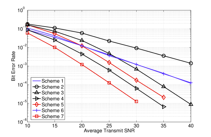
Figure 5: Performance comparison in a $(2,1,2,2)$ MARN, under 1 bit/user/channel use.

We first compare the BER of Scheme 1 with the other linear schemes (Schemes 2, 3, 4). In the $(2,1,2,2)$ MARN (Fig. 5), Schemes 3 and 4 achieve a diversity gain of 2, which is the int-free diversity gain. Schemes 1 and 2 achieve a diversity gain of 1 only. For this network, since the int-free condition is not satisfied, the proposed Scheme 1 performs worse than Scheme 4 for the entire simulated SNR range. Although it is worse than Scheme 3 for SNR larger than 27 dB due to the diversity loss, it outperforms Scheme 3 when the SNR is smaller than 27 dB due to its higher symbol rate. Compared with Scheme 2, the proposed scheme is superior for the simulated SNR range. At the BER level of $10^{-2}$, it is about 10 dB better. For the $(2,2,2,1)$ MARN (Fig. 6), the int-free condition is satisfied. The figure shows that Schemes 1 and 4 achieve a diversity gain of 2, while the diversity of Scheme 3 is slightly less than 2. This is because for Scheme 3, there is a $\log P$ factor in the error rate formula. As $P$ increases, the diversity should approach 2. For Schemes 1 and 4, the MRC and equalization eliminate the $\log P$ factor. Scheme 2 cannot be used for this network because the destination has only one antenna and cannot conduct full IC. The array gain of Scheme 1 is higher compared to both Schemes 3 and 4, since a lower-dimension constellation is used to achieve the same bit rate. At the BER level of $10^{-3}$, it is better than Schemes 3 and 4 by 10 dB and 5 dB, respectively. From the comparison, we can conclude that Scheme 1 is expected to outperform other linear schemes for MARNs satisfying the int-free condition, e.g., the $(2,2,2,1)$ MARN.

Next, we compare Scheme 1 with the schemes not satisfying the linear constraints (Schemes 5, 6, 7). Scheme 1 is first compared with Scheme 5. Scheme 5 achieves the int-free diversity from Table I, thus naturally having better BER than Scheme 1 in the high SNR regime for the $(2,1,2,2)$ MARN (Fig. 5). For SNR smaller than $20$ dB, Scheme 1 outperforms Scheme 5. In the $(2,2,2,1)$ MARN (Fig.6), where both schemes achieve the int-free diversity, Scheme 1 outperforms Scheme 5 in the entire SNR, e.g., it is about 6 dB better when BER$=10^{-3}$. The gain is obtained because in Scheme 1, user interference is avoided in the second step and the received signal quality is high. Then, Scheme 1 is compared with Scheme 6, which has additional decoding after IC. From both Fig. 5 and 6, we can observe that there is no diversity improvement by additional decoding after IC for Scheme 6. For the array gain, Scheme 6 outperforms in the low SNR regime (about 0.5 dB in Fig. 5 and 1.3 dB in Fig. 6); and has the same BER as Scheme 1 in the high SNR regime. This is because the BER performance is mainly restricted by interference in the high SNR regime. Finally, Scheme 1 is compared with Scheme 7, which allows joint decoding at the relay. We can see that joint decoding at the relay helps the network to achieve the int-free diversity, e.g., 2 in the $(2,1,2,2)$ MARN (Fig. 5), in addition to an improved array gain compared to Scheme 1, e.g., about 10 dB in the $(2,1,2,2)$ MARN (Fig. 5) and 2 dB in the $(2,2,2,1)$ MARN (Fig. 6). However, the relay needs to jointly decode both user’s symbols. Two symbols with 8PSK constellation are jointly recovered in the $(2,1,2,2)$ MARN, and four symbols with 8PSK constellation in the $(2,2,2,1)$ MARN. Since the relay does not need to decode in Scheme 1, the complexity of Scheme 7 is much higher compared to Scheme 1, especially in the $(2,2,2,1)$ MARN.

VI Conclusions

This paper is concerned with multi-user transmission and detection schemes for multi-access relay networks, in which multiple sources communicate with one destination by a common relay in two hops. For complexity considerations, the nodes in the network have two linear constraints: the relay generates its forward signals by linearly transforming its received signals; the destination has linear decoding complexity in the number of sources. A new scheme, called IC-Relay-TDMA, is proposed to cancel interference at the relay and forward the int-free observations of sources’ information in TDMA to the destination. IC-Relay-TDMA efficiently allows multi-users to communicate simultaneously in the first hop to enhance transmission rate. Through rigorous analysis and simulations, it is shown that IC-Relay-TDMA achieves diversity $\min\{J_{a}(R_{a}-J+1),R_{a}M\}$. When the number of destination antennas is no higher than $J_{a}(1-\frac{J-1}{R_{a}})$, the maximum int-free diversity $R_{a}M$ is achievable, with a higher symbol rate compared to the full-TDMA-DSTC scheme.

Appendix: Proof of Lemma 1

First, we show the scenario when the decoding in (18) is symbol-wise, i.e., $n=1$, then the scenario for multiple symbol joint decoding, i.e., $n\geq 2$.

For $n=1$, $\mathbf{H}_{n-1}=1$, ${\Sigma}_{\mathbf{u}}=\frac{c^{2}}{\gamma_{1}}+\frac{1}{\gamma_{g}}$, and $\mathbf{s}_{\mathrm{o}}^{(1)}=s_{1}^{(1)}$ from (18). The ML decoding is symbol wise. Let $\alpha=\frac{c^{2}}{2J_{a}}$, $\gamma={\Sigma}_{\mathbf{u}}^{-1}$, and $s_{1}^{(1)}-s_{1}^{(1)^{\prime}}=\Delta s_{1}^{(1)}$. The pairwise SER of decoding $s_{1}^{(1)}$ to $s_{1}^{(1)^{\prime}}$ can be written as

$$P(s_{1}^{(1)}\rightarrow s_{1}^{(1)^{\prime}})=\underset{f^{(j)}_{ki},g_{im}}{{\mathbb{E}}\,}Q\left(\sqrt{\alpha P\left|\Delta s_{1}^{(1)}\right|^{2}\gamma}\right),$$ (25)

where $Q(x)$ denotes the Gaussian Q function. Note that $Q(x)\geq\min\left\{\frac{1}{5}e^{-\frac{x^{2}}{2}},\frac{1}{3x}e^{-\frac{x^{2}}{2}}\right\}$ and both $\frac{1}{3x}e^{-\frac{x^{2}}{2}}$ and $\frac{1}{5}e^{-\frac{x^{2}}{2}}$ are decreasing functions. Thus, for any $\epsilon\geq 0$, $P(s_{1}^{(1)}\rightarrow s_{1}^{(1)^{\prime}})\geq P(\gamma\leq\epsilon)\min\left\{\frac{1}{5}e^{-\alpha P\Delta^{2}\epsilon},\frac{e^{-\alpha P\Delta^{2}\epsilon}}{3\sqrt{P\alpha\Delta^{2}\epsilon}}\right\}$ with $\Delta$ the minimum distance between any two constellation points. Let $\epsilon=P^{-1}$, we have $P(s_{1}^{(1)}\rightarrow s_{1}^{(1)^{\prime}})\geq P(\gamma\leq\epsilon)\underset{\zeta}{\underbrace{\min\left\{\frac{1}{5}e^{-\alpha\Delta^{2}},\frac{e^{-\alpha\Delta^{2}}}{3\sqrt{\alpha}\Delta}\right\}}}$, where $\zeta$ is a constant independent of $\epsilon$. Thus, diversity can be calculated as

$$d=-\lim_{P\rightarrow\infty}\frac{\log\ P(s_{1}^{(1)}\rightarrow s_{1}^{(1)^{\prime}})}{\log\ P}\leq\lim_{\epsilon\rightarrow 0^{+}}\frac{\log\ P(\gamma<\epsilon)+\log\ \zeta}{\log\ \epsilon}=\lim_{\epsilon\rightarrow 0^{+}}\frac{\log\ P(\gamma<\epsilon)}{\log\epsilon}.$$

This shows that the diversity is upperbounded by the right-hand-side (RHS) of (22). Next, we show that the diversity is also lowerbounded by the RHS of (22). Denote $\beta$ as the maximum distance between any two constellation points. For any $\epsilon\geq 0$, using the Chernoff bound on SER and noticing that $e^{-\frac{\beta^{2}\alpha P\gamma}{2}}$ is a decreasing function with $\gamma$, we have

$$P(s_{1}^{(1)}\rightarrow s_{1}^{(1)^{\prime}})<\underset{\gamma}{{\mathbb{E}}\,}e^{-\frac{\beta^{2}\alpha P\gamma}{2}}=\int_{0}^{\epsilon}e^{-\frac{\beta^{2}\alpha P\gamma}{2}}f(\gamma)d\gamma+\int_{\epsilon}^{\infty}e^{-\frac{\beta^{2}\alpha P\gamma}{2}}f(\gamma)d\gamma<P(\gamma<\epsilon)+e^{-\frac{\beta^{2}\alpha P\epsilon}{2}},$$ (26)

where $f(\gamma)$ is the probability density function of $\gamma$. Let $\epsilon=P^{-n},0<n<1$. As $P$ increases, the RHS of (26) is dominated by $P(\gamma<\epsilon)$. The diversity can be lowerbounded as $d\geq\underset{{\epsilon\rightarrow 0^{+}}}{\lim}\frac{n\log P(\gamma<\epsilon)}{\log\ \epsilon}$. Since $n$ can be chosen very close to $1$, the lowerbound and upperbound converge.

Now, we consider the case of $n>1$. Denote $\Delta\mathbf{s}_{\mathrm{o}}^{(1)}=\mathbf{s}_{\mathrm{o}}^{(1)}-\mathbf{s}_{\mathrm{o}}^{(1)^{\prime}}$. The pairwise error probability of decoding a vector of $2^{n-1}$ symbols $\mathbf{s}_{\mathrm{o}}^{(1)}$ to $\mathbf{s}_{\mathrm{o}}^{(1)^{\prime}}$ in the ML decoding in (18) can be written as

$$P\left(\mathbf{s}_{\mathrm{o}}^{(1)}\rightarrow\mathbf{s}_{\mathrm{o}}^{(1)^{\prime}}\right)=\underset{f_{ki}^{(j)},g_{im}}{{\mathbb{E}}\,}Q\left(\sqrt{\alpha P\underset{\Gamma}{\underbrace{\Delta\mathbf{s}_{\mathrm{o}}^{(1)*}\mathbf{H}_{n-1}^{*}\mathbf{\Sigma}_{\mathbf{u}}^{-1}\mathbf{H}_{n-1}\Delta\mathbf{s}_{\mathrm{o}}^{(1)}}}}\right).$$ (27)

Since $\mathbf{H}_{n-1}^{*}\mathbf{\Sigma}_{\mathbf{u}}^{-1}\mathbf{H}_{n-1}\prec{\rm tr}\,\{\mathbf{H}_{n-1}^{*}\mathbf{\Sigma}_{\mathbf{u}}^{-1}\mathbf{H}_{n-1}\}\mathbf{I}_{2^{n-1}}$, we have that $\Gamma<{\rm tr}\,\{\mathbf{H}_{n-1}^{*}\mathbf{\Sigma}_{\mathbf{u}}^{-1}\mathbf{H}_{n-1}\}\|\Delta\mathbf{s}_{\mathrm{o}}^{(1)}\|^{2}<2^{n-1}{\rm tr}\,\{\mathbf{H}_{n-1}^{*}\mathbf{\Sigma}_{\mathbf{u}}^{-1}\mathbf{H}_{n-1}\}\beta^{2}$ with $\beta$ the maximum distance between any two points in all constellations. Thus, a lowerbound on (27) can be obtained as $P_{l}=Q\left(\sqrt{{\alpha 2^{n-1}P}{\rm tr}\,\{\mathbf{H}_{n-1}^{*}\mathbf{\Sigma}_{\mathbf{u}}^{-1}\mathbf{H}_{n-1}\}\beta^{2}}\right)$. The diversity of $P_{l}$ upperbounds that of $P\left(\mathbf{s}_{\mathrm{o}}^{(1)}\rightarrow\mathbf{s}_{\mathrm{o}}^{(1)^{\prime}}\right)$. Recall that $P_{l}$ is similar to (25). The diversity of the lowerbound can be evaluated by (22) using ${\rm tr}\,\{\mathbf{H}_{n-1}^{*}\mathbf{\Sigma}_{\mathbf{u}}^{-1}\mathbf{H}_{n-1}\}$ as the instantaneous normalized receive SNR. Thus, the diversity obtained by using $\gamma={\rm tr}\,\{\mathbf{H}_{n-1}^{*}\mathbf{\Sigma}_{\mathbf{u}}^{-1}\mathbf{H}_{n-1}\}$ in (22) upperbounds that of $P\left(\mathbf{s}_{\mathrm{o}}^{(1)}\rightarrow\mathbf{s}_{\mathrm{o}}^{(1)^{\prime}}\right)$.

Next, we find the lowerbound on the diversity of $P\left(\mathbf{s}_{\mathrm{o}}^{(1)}\rightarrow\mathbf{s}_{\mathrm{o}}^{(1)^{\prime}}\right)$. Since the entries of $\mathbf{s}_{\mathrm{o}}^{(1)}$ are collected from finite constellations satisfying (1), there exists a positive number $\theta$ that lowerbounds all $\left|\mathbf{h}_{l}\Delta\mathbf{s}_{\mathrm{o}}^{(1)}\right|^{2}$. Noticing that $\mathbf{\Sigma}_{\mathbf{u}}$ is diagonal from (19). We have $\Gamma=\underset{l=1:2^{n-1}}{\sum}\lambda_{l}^{-1}\left|\mathbf{h}_{l}\Delta\mathbf{s}_{\mathrm{o}}^{(1)}\right|^{2}>\underset{l=1:2^{n-1}}{\sum}\lambda_{l}^{-1}\theta^{2}={\rm tr}\,\{\mathbf{H}_{n-1}^{*}\mathbf{\Sigma}_{\mathbf{u}}^{-1}\mathbf{H}_{n-1}\}\frac{\theta^{2}}{2^{n-1}}$ with $\lambda_{l}$ the $l$-th diagonal entry of $\mathbf{\Sigma}_{\mathbf{u}}$. Therefore, the diversity obtained by using $\gamma={\rm tr}\,\{\mathbf{H}_{n-1}^{*}\mathbf{\Sigma}_{\mathbf{u}}^{-1}\mathbf{H}_{n-1}\}$ in (22) lowerbounds that of $P\left(\mathbf{s}_{\mathrm{o}}^{(1)}\rightarrow\mathbf{s}_{\mathrm{o}}^{(1)^{\prime}}\right)$. The diversity of $P\left(\mathbf{s}_{\mathrm{o}}^{(1)}\rightarrow\mathbf{s}_{\mathrm{o}}^{(1)^{\prime}}\right)$ can be calculated by using $\gamma={\rm tr}\,\{\mathbf{H}_{n-1}^{*}\mathbf{\Sigma}_{\mathbf{u}}^{-1}\mathbf{H}_{n-1}\}$ in (22).

TABLE I: Performance comparison in $(J,J_{a},R_{a},M)$ MARNs.

Scheme	Concurrent Transmission	Diversity	Symbol Rate	Linearity
IC-Relay-TDMA	only the user-relay link	$\min\{J_{a}(R_{a}-J+1),R_{a}M\}$	$\frac{R_{o}}{J+R_{o}}$	Yes
full-TDMA-DSTC	none	$R_{a}\min\{J_{a},M\}$	$\frac{R_{o}}{J(1+R_{o})}$	Yes
DSTC joint-user ML decoding	both links	$R_{a}\min\{J_{a},M\}$	$\frac{1}{2}$	No
DSTC-ICRec	both links	$\min\{J_{a},M-1\}$ for $J=2,J_{a}=1,2,R_{a}=2$	$\frac{1}{2}$	Yes

Figure 2: General Multi-user cooperative networks. The dash line denotes communication flows and the solid lines denote physical links.

Figure 3: Block diagram for IC-Relay-TDMA.

References

- [1] J. Laneman and G. Wornell, “Distributed space-time-coded protocols for exploiting cooperative diversity in wireless network,” IEEE Tran. on Info. Theory, vol. 49, pp. 2415–2425, Oct. 2003.
- [2] Y. Jing and B. Hassibi, “Distributed space-time coding in wireless relay networks,” IEEE Trans. on Wireless Comm., vol. 5, pp. 3524–3536, Dec. 2006.
- [3] K. Azarian, H. Gamal, and P. Schniter, “On the achievable diversity-multiplexing tradeoff in half-duplex cooperative channels,” IEEE Trans. on Info. Theory, vol. 51, pp. 4152–4172, Dec. 2005.
- [4] J. Laneman, D. Tse, and G. Wornell, “Cooperative diversity in wireless networks: Efficient protocols and outage behavior,” IEEE Trans. on Info. Theory, vol. 50, pp. 3062–3080, Dec. 2004.
- [5] V. Morgenshtern, H. Bolcskei, and R. Nabar, “Distributed orthogonalization in large interference relay networks,” in Proc. of International Symposium on Information Theory, 2005., Adelaide, Australia, Sep. 2005, pp. 1211 –1215.
- [6] A. Wittneben and B. Rankov, “Distributed antenna systems and linear relaying for gigabit MIMO wireless,” in Proc. of IEEE Vehicular Technology Conference VTC, Los Angeles, USA, Fall 2004.
- [7] A. Wittneben, “Coherent multiuser relaying with partial relay cooperation,” in Proc. of IEEE WCNC, Las Vegas, NV, USA, Apr. 2006.
- [8] B. Niu, O. Simeone, O. Somekh, and A. M. Haimovich, “Throughput of two-hop wireless networks with relay cooperation,” in Proc. of Allerton Conference, Monticello, IL, Sep. 2007.
- [9] S. Berger and A. Wittneben, “Cooperative distributed multiuser MMSE relaying in wireless Ad-Hoc networks,” in Asilomar Conference on Signals, Systems, and Computers 2005, Pacific Grove, CA, Nov. 2005.
- [10] A. El-Keyi and B. Champagne, “Cooperative MIMO-beamforming for multiuser relay networks,” in Proc. of IEEE ICCASP, Las Vegas, NV, Apr. 2008.
- [11] Y. Jing and B. Hassibi, “Diversity analysis of distributed space-time codes in relay networks with multiple transmit/receive antennas,” EURASIP Jour. on Advances in Signal Proc., vol. 2008, 2008, article ID 254573, 17 pages, doi:10.1155/2008/254573.
- [12] A. O. Yilmaz, “Cooperative multiple-access in fading relay channels,” in Proc. of IEEE ICC, Istanbul, Turkey, Jun. 2006.
- [13] Y. Jing and H. Jafarkhani, “Interference cancellation in distributed space-time coded wireless relay networks,” in Proc. of IEEE ICC, 2009.
- [14] A. Naguib, N. Seshadri, and A. Calderbank, “Applications of space-time block codes and interference suppression for high capacity and high data rate wireless systems,” in Proc. of Asilomar Conf., Pacific Grove, CA, Oct. 1998.
- [15] A. Stamoulis, N. Al-Dhahir, and A. Calderbank, “Further results on interference cancellation and space-time block codes,” in Proc. of Asilomar Conf., Pacific Grove, CA, Oct. 2001.
- [16] J. Kazemitabar and H. Jafarkhani, “Multiuser interference cancellation and detection for users with more than two transmit antennas,” IEEE Trans. on Comm., pp. 574–583, Apr. 2008.
- [17] L. Li, Y. Jing, and H. Jafarkhani, “Multi-user transmissions for relay networks with linear complexity,” http://arxiv.org/abs/1007.3315, Jul. 2010.
- [18] S. Sun and Y. Jing, “Channel training and estimation in distributed space-time coded relay networks with multiple transmit/receive antennas,” in Proc. of IEEE WCNC, Sydney, Australia, Apr. 2010.
- [19] S. Barghi, H. Jafarkhani, and H. Yousefi’zadeh, “MAC/PHY cross-layer design and analysis for multiple packet detector MIMO,” in Proc. IEEE ICC, Cape Town, South Africa, May 2010.
- [20] O. Tirkkonen, A. Boariu, and A. Hottinen, “Minimal nonorthogonality rate 1 space-time block code for 3+ Tx antennas,” in Proc. IEEE 6th Int. Symp. Spread-Spectrum Techniques and Applications (ISSSTA 2000), Parsippany, NJ, USA, Sep. 2000.
- [21] H. Jafarkhani, “A quasi-orthogonal space-time block codes,” IEEE Transactions on Communications, vol. 49, pp. 1– 4, Jan. 2001.
- [22] N. Sharma and C. Papadias, “Improved quasi-orthogonal codes through constellation rotation,” IEEE Transactions on Communications, vol. 51, no. 3, pp. 332 – 335, Mar. 2003.
- [23] W. Su and X.-G. Xia, “Signal constellations for quasi-orthogonal space-time block codes with full diversity,” IEEE Transactions on Information Theory, vol. 50, no. 10, pp. 2331 – 2347, Oct. 2004.
- [24] Y. Jing, “Improving distributed space-time coding through combining at the multiple-antenna relay,” in IEEE Workshop on Computational Advances in Multi-Sensor Adaptive Processing, Dec. 2009.
- [25] V. Tarokh, H. Jafarkhani, and A. Calderbank, “Space-time block codes from orthogonal designs,” IEEE Transactions on Information Theory, vol. 45, pp. 1456–1467, Jul. 1999.
- [26] H. Jafarkhani, Space-Time Coding: Theory and Practice. Cambridge University Press, 2005.
- [27] J. Kazemitabar and H. Jafarkhani, “Performance analysis of multiple-antenna multi-user detection,” Information Theory and Applications Workshop, Jan. 2009.
- [28] L. Li, Y. Jing, and H. Jafarkhani, “Diversity results for DSTC-ICRec and Joint-user ML decoding,” http://webfiles.uci.edu/liangbil/papers/div.pdf, Mar. 2010.
- [29] Y. Jing and H. Jafarkhani, “Using orthogonal and quasi-orthogonal designs in wireless relay networks,” IEEE Trans. on Info. Theory, pp. 4106–4118, Nov. 2007.