Strong magnetohydrodynamic turbulence with cross helicity

Abstract

Magnetohydrodynamics (MHD) provides the simplest description of magnetic plasma turbulence in a variety of astrophysical and laboratory systems. MHD turbulence with nonzero cross helicity is often called imbalanced, as it implies that the energies of Alfvén fluctuations propagating parallel and anti-parallel the background field are not equal. Recent analytical and numerical studies have revealed that at every scale, MHD turbulence consists of regions of positive and negative cross helicity, indicating that such turbulence is inherently locally imbalanced. In this paper, results from high resolution numerical simulations of steady-state incompressible MHD turbulence, with and without cross helicity are presented. It is argued that the inertial range scaling of the energy spectra ($E^{\pm}$) of fluctuations moving in opposite directions is independent of the amount of cross-helicity. When cross helicity is nonzero, $E^{+}$ and $E^{-}$ maintain the same scaling, but have differing amplitudes depending on the amount of cross-helicity.

I Introduction

Magnetohydrodynamic (MHD) equations govern the dynamics of a plasma when the spatial scales of interest greatly exceed any intrinsic plasma scale. The MHD model is relevant in understanding waves, instabilities, and turbulence in a variety of astrophysical systems. For instance, magnetohydrodynamic (MHD) turbulence plays a key role in the theoretical modeling of the spectra of velocity and magnetic fluctuations in the Solar Wind (e.g., Coleman, 1966, 1968; Belcher and Davis, 1971; Marsch, 1991; Goldstein et al., 1995) as well as electron density fluctuations in the interstellar medium (e.g., Armstrong et al., 1995; Lithwick and Goldreich, 2001).

Theoretical modeling of the spectra in strong MHD turbulence has developed on different fronts: phenomenology, statistical closures and more recently, high-resolution numerical simulations. The first phenomenological model, a la Kolmogorov Kolmogorov (1941); Obukhov (1941), of the energy spectrum was developed independently by Iroshnikov (Iroshnikov, 1963) and Kraichnan (Kraichnan, 1965). In these works they realized that the magnetic field of the large scale eddies acts in much the same way as a guide field that supports smaller scale Alfvénic fluctuations, and the turbulent energy transfer takes place as the result of many cumulative collisions between counter-propagating Alfvén wave packets traveling along the local magnetic field. One deficiency of this phenomenology is that it is based on the assumption of an isotropic spectral transfer, in contradiction with more recent results that reveal the anisotropic character of MHD turbulence (e.g., Montgomery and Turner, 1981; Shebalin et al., 1983). To account for anisotropy in the strong turbulence regime, Goldreich and Sridhar (Goldreich and Sridhar, 1995), hereafter referred as GS, proposed a new phenomenology in which they introduced the so-called critical balance condition, stating that the turbulence is strong when the time scale for wave propagation along the magnetic field matches the nonlinear interaction time. In the past decade, constantly increasing massively parallel computer clusters have become large enough to allow one to simulate the inertial range spectra of strong MHD turbulence, leading to an extensive volume of work addressing universal scaling laws in MHD turbulence (e.g., Cho and Vishniac, 2000; Maron and Goldreich, 2001; Haugen et al., 2003; Biskamp, 2003; Müller and Grappin, 2005; Mason et al., 2006, 2008; Mininni and Pouquet, 2007; Beresnyak and Lazarian, 2008; Perez and Boldyrev, 2008, 2009). These simulations have motivated new phenomenological models and have resulted in a renewed interest in the fundamentals of MHD turbulence.

One aspect of MHD turbulence, which has recently drawn significant attention is the role that cross-helicity plays in the turbulent cascade (Lithwick et al., 2007; Chandran, 2008; Beresnyak and Lazarian, 2009; Perez and Boldyrev, 2009; Podesta and Bhattacharjee, ; Perez and Boldyrev, 2010). Both total energy $E=\frac{1}{2}\int(v^{2}+b^{2})d^{3}x$ and total cross-helicity $H^{c}=\int({\bf v}\cdot{\bf b})d^{3}x$ are conserved by nonlinear interactions; where ${\bf v}$ and ${\bf b}$ are velocity and magnetic fields. In MHD turbulence both energy and cross helicity cascade from large to small scales as a result of the nonlinear interaction of counter-propagating Alfvén fluctuations. If we denote $E^{\pm}=\frac{1}{4}\int({\bf v}\pm{\bf b})^{2}\,d^{3}x$, which are the energies carried by Alfvén fluctuations propagating in opposite directions (the details are given below), the total energy and cross-helicity of the system are given by $E=E^{+}+E^{-}$ and $H_{c}=E^{+}-E^{-}$, respectively. Therefore, when the latter is nonzero, the energies of waves propagating along and against the guide field are not equal, and in that sense the turbulence is called imbalanced.

Independent numerical simulations by different groups have demonstrated that strong MHD turbulence is always locally imbalanced, in the sense that in the steady state, the turbulence develops correlated regions of positive and negative cross-helicity, irrespective of the overall cross-helicity of the system. Imbalance turbulence is also present in the solar wind, where velocity and magnetic fluctuations show high correlations of a preferred sign, that is, the normalized cross-helicity $\sigma_{c}={\left\langle\mathbf{v}\cdot\mathbf{b}\right\rangle}/{E}={H_{c}}/{E}$ is close to unity. The preferred positive sign of $\sigma_{c}$ indicates that there is more energy in Alfvén waves propagating outwards from the Sun than propagating inwards Belcher and Davis (1971).

Recently, several phenomenological models have addressed steady-state strong imbalanced MHD turbulence Lithwick et al. (2007); Beresnyak and Lazarian (2008); Chandran (2008); Perez and Boldyrev (2009); Podesta and Bhattacharjee , some with support from numerical simulations and observations. However, these models have lead to conflicting predictions. For instance, the theories by Lithwick et al Lithwick et al. (2007) and Beresnyak and Lazarian Beresnyak and Lazarian (2008) conclude that in imbalanced regions the Elsässer spectra have the same scalings $E^{+}(k_{\perp})\propto E^{-}(k_{\perp})\propto k_{\perp}^{-5/3}$. The theory by Chandran Chandran (2008) proposes that the spectra of $E^{+}(k_{\perp})$ and $E^{-}(k_{\perp})$ are different depending of the degree of imbalance. Finally, the analysis by Perez & Boldyrev Perez and Boldyrev (2009) and Podesta & Bhattacharjee Podesta and Bhattacharjee finds that the spectra of $E^{+}(k_{\perp})$ and $E^{-}(k_{\perp})$ have different amplitudes but the same scalings $E^{+}(k_{\perp})\propto E^{-}(k_{\perp})\propto k_{\perp}^{-3/2}$.

In this work we present results from high resolution direct numerical simulations of strong and steadily driven MHD turbulence, aimed to elucidate the role of cross-helicity and resolve the controversies among different theories. Hereafter, strong turbulence is defined in the sense of Golreich and Sridhar Goldreich and Sridhar (1995). This paper is organized as follows. Section II briefly describes the MHD equations and the relevance of using the Reduced MHD model for strong turbulence simulations. Section III describes in detail the proposed numerical strategy and discusses important numerical aspects that need to be considered when simulating strong imbalanced MHD turbulence. In section IV, the most relevant results from an extensive number of numerical simulations are presented. In section V a phenomenological model for the simulation results is proposed and section VI presents the conclusions.

II Model equations

In the presence of a guide field ${\bf B_{0}}$, the incompressible MHD equations describing the evolution of magnetic and velocity fluctuations, ${\bf b}(\mathbf{x},t)$ and ${\bf v}(\mathbf{x},t)$, can be written in terms of the so-called Elsässer variables Elsasser (1956), ${\bf z}^{\pm}={\bf v}\pm{\bf b}$:

$$\left(\frac{\partial}{\partial t}\mp{\bf v}_{A}\cdot\nabla\right){\bf z}^{\pm}+\left({\bf z}^{\mp}\cdot\nabla\right){\bf z}^{\pm}=-\nabla P+\nu\nabla^{2}\mathbf{z}^{\pm}+{\bf f}^{\pm},$$ (1)

where ${\bf v}_{A}={\bf B}_{0}/\sqrt{4\pi\rho}$ is the Alfvén velocity, $\rho$ is the fluid density, $P$ is the total pressure that is determined from the incompressibility condition, $\nabla\cdot{\bf z}^{\pm}=0$, ${\bf f^{\pm}}$ are large-scale forcing, and $\nu$ is the viscosity which acts as an energy sink at small scales. In contrast with a uniform flow in hydrodynamic, which can be removed by a Galilean transform, the guide magnetic field, whether imposed externally or created by large-scale fluctuations, is essential in MHD turbulence. It cannot be removed by Galilean transform and it mediates nonlinear interactions at all smaller scales. The linear terms, $({\bf v}_{A}\cdot\nabla){\bf z}^{\pm}$, describe advection of Alfvén wave packets along the guide field, while the nonlinear interaction terms, $\left({\bf z}^{\mp}\cdot\nabla\right){\bf z}^{\pm}$, are responsible for energy redistribution over scales. It can be observed from equations (1) that nonlinear interactions can only occur between $\mathbf{z}^{+}$ and $\mathbf{z}^{-}$, and such interactions take place when the fields overlap or “collide” with each other. It is convenient to describe the resulting energy spectra in terms of the so-called Elsässer energies, defined as $E^{\pm}=\int|{\bf z}^{\pm}|^{2}d^{3}x/4$.

In the limit of small amplitude of fluctuations, the incompressible MHD system (1) describes non-interacting linear Alfvén waves with dispersion relation $\omega^{\pm}(\mathbf{k})=\pm k_{\|}v_{A}$. The incompressibility condition requires these waves to be transverse, and they are typically decomposed into two polarizations, the shear-Alfvén wave ($\mathbf{z}^{\pm}_{S}$) and the pseudo-Alfvén waves ($\mathbf{z}^{\pm}_{P}$) given in Fourier space

$$\mathbf{e}_{S}\equiv\frac{\mathbf{e}_{\|}\times\mathbf{k}}{k_{\perp}},\quad\mathbf{e}_{P}\equiv\frac{\mathbf{k}\times\mathbf{e}_{S}}{k},$$ (2)

where ${\bf e}_{\|}$ is the unit vector in the direction of the guide field. Strong MHD turbulence is dominated by fluctuations with $k_{\perp}\gg k_{\|}$. Goldreich and Sridhar (1995) argued that since for large $k_{\perp}$ the polarization of the pseudo-Alfvén fluctuations is almost parallel to the guide field, such fluctuations are coupled only to field-parallel gradients, which are small since $k_{\|}\ll k_{\perp}$. Therefore, the pseudo-Alfvén modes do not play a dynamically essential role in the turbulent cascade. We can remove the pseudo-Alfvén modes by setting $\mathbf{z}^{\pm}_{\|}=0$ in equations (1) to obtain

$$\partial_{t}{\tilde{\bf z}}^{\pm}\mp({\bf V}_{A}\cdot\nabla){\tilde{\bf z}}^{\pm}+({\tilde{\bf z}}^{\mp}\cdot\nabla){\tilde{\bf z}}^{\pm}=-\nabla_{\perp}P+\frac{1}{R}\nabla^{2}{\tilde{\bf z}}^{\pm},$$ (3)

where $R$ denotes the Reynolds numbers (discussed below). In this system, the fluctuating fields have only two vector components, ${\tilde{\bf z}}^{\pm}=\{{\tilde{z}}^{\pm}_{1},{\tilde{z}}^{\pm}_{2},0\}$ (where we chose the $z$ axis along the guide field $B_{0}$) but depend on all three spatial coordinates. It can be demonstrated that system (3) is equivalent to the Reduced MHD model, originally developed for tokamak plasmas by Kadomtsev and Pogutse (1974) and Strauss (1976).

III Numerical approach

The reduced MHD model  (3) describing the nonlinear interactions of Shear-Alfvén modes is a valuable tool in theoretical and numerical studies of incompressible MHD turbulence. Based on this model, we now discuss the conditions that should be satisfied in order to correctly simulate strong MHD turbulence, both balanced and imbalanced.

III.1 Computational domain

In the presence of a strong guide field, MHD turbulence is inherently anisotropic. It is important to point out that such anisotropy will develop deep in the inertial range even if it is not present at the outer scale where the turbulence is driven. This can be understood from the Golreich and Sridhar Goldreich and Sridhar (1995) picture of strong turbulence. As the turbulence cascades to smaller scales, eddies become more and more shrunk in the field-perpendicular direction until fluctuations satisfy the critical balance condition $k_{\|}B_{0}\sim k_{\perp}b_{\lambda}$, where $k_{\|}\sim 1/l$ and $k_{\perp}\sim 1/\lambda$ are the field-parallel and field-perpendicular wave vectors associated with an anisotropic eddy of parallel size $l$ and perpendicular size $\lambda$, respectively, and $b_{\lambda}$ denoted rms magnetic fluctuations at scale $\lambda$. It is assumed that $b_{\lambda}\sim v_{\lambda}$.

In a traditional cubic simulation box, when an anisotropic wave packet fits the field-parallel direction ($z-$dimension of the box) its field-perpendicular dimensions are much smaller than the $x$ and $y$ dimensions of the box. This is obviously not an optimal situation, since the field-perpendicular resolution required to resolve such a wave packet should be much higher than the field-parallel resolution. This decreases the effective field-perpendicular resolution of the simulations. For example, in the case a cubic $512^{3}$ box with the guide field $B_{0}=5b_{rms}$, one will have an equivalent field-perpendicular resolution of only $512/5\sim 100$.

For our simulations, we define the nonlinear interaction strength parameter

$$\chi=(k_{\perp}b_{\lambda})/(k_{\|}B_{0}),$$ (4)

so that the critical balance condition then implies $\chi\sim 1$.

Simulations of steadily-driven (dissipative) incompressible turbulence are generally based on the Fourier pseudo-spectral method. As with any spectral method, the solution to the differential equation is approximated by a truncated Fourier expansion, and the partial differential equation is converted to a set of ordinary differential equations in time for the $N$ Fourier coefficients. Nonlinear terms in this representation become convolutions whose direct computation requires $O(N^{2})$ operations. In pseudo-spectral methods, the convolutions are computed in real (or configuration) space by means of a Fast Fourier Transform (FFT) that only requires $O(NlogN)$ operations. For the numerical simulations presented in this work, a third order semi-implicit Runge-Kutta/Crank-Nicholson method was used for the time integration.

In order to allow for the inertial interval to develop, turbulence is driven at the lowest resolvable wave numbers, and the energy dissipates at large wave numbers determined by the Reynolds numbers. For simulations on a cubic periodic box of size $L$, the smallest wave-numbers along the field-parallel and field-perpendicular directions coincide, i.e., $k_{\perp}=k_{\|}=2\pi/L$. Therefore, driving at the low $k_{\|},k_{\perp}$ results in an isotropic forcing and the nonlinear strength parameter at the forcing scale becomes $\chi_{0}={k_{\perp}b_{\lambda}}/{k_{\|}B_{0}}\sim{b_{\lambda}}/{B_{0}}\ll 1$, which means that at least at the large scales, nonlinear interactions are weak. This would not be harmful if we had the resources to achieve arbitrarily high resolution, as the turbulence would proceed weakly until $\chi\sim 1$, and then it would become strong. However, simulations generally produce a rather limited inertial range, so that the parameter $\chi$ can hardly reach unity in such a setup.

As pointed out by Maron and Goldreich (2001), and applied in recent simulations Mason et al. (2006, 2008); Perez and Boldyrev (2008), an effective way to avoid this is to use an anisotropic domain such that at the forcing scale the parameter $\chi$ is already of order unity, that is, the excited large-scale modes are already anisotropic and satisfy the critical balance condition. To achieve this we choose an elongated box $L_{\perp}^{2}\times L_{\|}$, so that the lowest field-perpendicular and field-parallel wave-numbers are $k_{\perp}=2\pi/L_{\perp}$ and $k_{\|}=2\pi/L_{\|}$, respectively. In this case, forcing at the lowest $k_{\perp},k_{\|}$ leads to $\chi_{0}=(L_{\|}b_{\lambda})/(L_{\perp}B_{0}),$ which is of order unity provided that

$${L_{\perp}}/{L_{\|}}\sim{b_{\lambda}}/{B_{0}}.$$ (5)

In this way, the turbulence is excited in a strong regime and the cascade proceeds down to smaller scales preserving the critical balance condition.

III.2 Numerical Resolution

At first sight, it appears that elongating the box along the $z$ direction to match the elongation of the eddies should not change the number of grid points required in this direction compared to the number of points in the $x$ direction. Fortunately, the number of points in the $z$ direction can be reduced. This follows from the fact that the turbulent spectrum declines quite slowly, as a power-law, in the $k_{\perp}$ direction, while it drops sharply in the $k_{\|}$ direction for $k_{\|}>k_{\perp}^{\alpha}$, where $\alpha$ is a some positive power not exceeding 1 (Cho and Vishniac, 2000; Maron and Goldreich, 2001; Oughton et al., 2004; Perez and Boldyrev, 2008, 2009) . This qualitatively different spectral behavior in $k_{\|}$ and $k_{\perp}$ directions allows one to reduce the numerical resolution by a factor of 2 to 4 in the parallel direction, see Table 1. We checked that the restoration of the full resolution in the z direction does not change the results, while significantly increases the computing costs.

III.3 Periodic Boundary Conditions

The spectral method assumes periodic boundary conditions in all spatial directions. The periodic boundary conditions in the direction of the guide field (the $z-$direction) may raise the question of whether the magnetic field lines are periodic in such numerical simulations. If they were periodic then the Alfvén modes counter-propagating along a given magnetic field line would repeatedly interact only among themselves, and, therefore, they might not become sufficiently decorrelated between the consequent interactions. To answer this question we note that the numerical setup ensures periodicity of the fluctuations ${\bf b}$, but not the magnetic field lines. Magnetic field lines are integral lines of a magnetic field, therefore, they are generally not periodic in the $z-$direction, since ${\bf b}({\bf k}_{\|}=0)$ is generally nonzero. Consequently, an eddy traveling along a magnetic field line interacts with many independent counter-propagating eddies. Reducing the parallel box size $L_{\|}$ may however lead to artificial overlap of an elongated eddy with itself. This may explain why reducing the parallel box size $L_{\|}$ below (5) somewhat spoils the spectrum at low wave numbers, as seen in forced simulations of Müller & Grappin (Müller and Grappin, 2005). Increasing $L_{\|}$ beyond (5) does not change the results but increases the computational cost [Mason & Cattaneo, private communication 2006].

III.4 The strength of the guide field

In the inertial interval of turbulence, the guide field should be strong compared to the turbulent fluctuations, $b_{\lambda}\ll B_{0}$. It is important to establish how small the fluctuations should be in order to exhibit the universal turbulent spectrum. The question is especially relevant for numerical simulations, as the large guide field implies small Alfvénic time and, therefore, large computing cost. This problem was numerically addressed in Mason et al. (2006), where it was found that the transition to the universal regime occurs approximately at $b_{\lambda}/B_{0}\sim 1/3$. For $b_{\lambda}/B_{0}>1/3$ the energy spectrum is closer to $-5/3$, possibly indicating that the magnetic field does not qualitatively change the Kolmogorov dynamics for the scales attainable in the numerical simulations. For $b_{\lambda}/B_{0}<1/3$, the guide field significantly affects the dynamics, and the spectrum changes to $-3/2$. The “sweet spot” often used in numerical simulations is $b_{rms}/B_{0}\sim 1/5$; it has been checked that the smaller ratio, $b_{\lambda}/B_{0}\sim 1/10$, does not lead to noticeably different results (see for example  Müller and Grappin (2005); Mason et al. (2006, 2008)).

It is also important to note that in numerical simulations, where inertial intervals have quite limited extent, the condition $b_{rms}/B_{0}<1/3$ should be satisfied at the outer scale. Indeed, since $b_{\lambda}$ decreases with the scale quite slowly, say $b_{\lambda}\propto\lambda^{1/3}$, if the condition $b_{rms}/B_{0}<1/3$ is not satisfied at the outer scale, it can hardly be satisfied in the inertial interval.

III.5 Reynolds numbers

Probably the most significant limitation on numerical simulations is imposed by the consideration of imbalanced turbulence. Indeed, in the imbalanced case, $\gamma=z^{+}/z^{-}>1$, the formally constructed Reynolds numbers $Re_{\lambda}^{\pm}=\lambda z_{\lambda}^{\mp}/\nu$ corresponding to $\mathbf{z}^{+}$ and $\mathbf{z}^{-}$ fields at some scale $\lambda$ would be essentially different (here $z^{\pm}\equiv|\mathbf{z}^{\pm}|$). One can argue that the effective Re number is then the smaller of the two, see below. Therefore, the resolution requirements increase with the amount of imbalance in order to produce large inertial ranges. Assume that the number of grid points in a field-perpendicular direction scales with the Reynolds number as $N\sim Re^{\beta}$, where $\beta=2/3$ or $3/4$ depending on the spectral slope ($3/2$ or $5/3$). Then increasing the imbalance $\gamma$ by, say, a factor of 3 will require increasing the resolution by approximately a factor of 2. Noting that resolution of at least 1024 is required to simulate the imbalance $\gamma\sim 2$ (see below), we conclude that significantly stronger imbalance is not achievable with present day computing power.

III.6 Random Forcing

Another question that arises in the strong turbulence regime concerns the type of forcing. In real systems, large-scale turbulence can be driven by instabilities exciting both velocity and magnetic harmonics, by external antennae exciting magnetic fields, etc.; this should not matter for the spectrum of small-scale fluctuations. Similarly, in numerical simulations one can force at large scales either velocity or magnetic field, or both of them, this does not change the result (Mason et al., 2008). The goal is therefore not to mimic any real-life driving but rather to optimize the transition to the inertial interval.

In this section we discuss the important aspects to be considered when choosing a particular forcing. We assume a random force ${\tilde{\bf f}}$ that has no component along $z$, it is solenoidal in the $x-y$ plane and its Fourier coefficients outside the range

$$1\leq k_{\perp}\leq 2,\quad(2\pi/L_{\|})\leq k_{\|}\leq(2\pi/L_{\|})n_{z}$$ (6)

are zero, where $n_{z}$ determines the width of the force spectrum in $k_{\|}$, and $L_{\perp}=2\pi$. The Fourier coefficients inside that range are Gaussian random numbers with amplitude chosen so that the resulting rms velocity fluctuations are of order unity. The individual random values are refreshed independently at time intervals $\tau$. The parameter $n_{z}$ controls the degree to which the critical balance condition is satisfied at the forcing scale. Note that we do not drive the $k_{\|}=0$ mode but allow it to be generated by nonlinear interactions.

Figure 1: Field-parallel energy spectrum at the dominant mode $k_{\perp}=3$ for different forcing correlation times. The dotted line represents the normalized spectrum of the forcing. We observe that as the correlation time increases, large $k_{\|}$ modes get suppressed despite the fact that force amplitude is the same for all modes.

In contrast with incompressible hydrodynamic system, an incompressible MHD system can support Alfvén waves. When the system is driven by a time dependent forcing, the most effectively driven modes are those resonating with the frequencies present in the forcing. Therefore, the spatial spectra of the large-scale velocity and magnetic fluctuations are not generally the same as the spatial spectrum of the force. Rather, they essentially depend on the both spatial and temporal spectra of the random forcing. Ultimately, it is the spectrum of the large-scale velocity and magnetic fluctuations, not the driving force, that should be controlled in numerical simulations. To illustrate this we performed a series of simulations in which we drive the modes given by equation (6) with $n_{z}=8$. We would expect this to excite all modes from $k_{0\|}=(2\pi/L_{z})$ to $8k_{0\|}$. Figure 1 shows the field-parallel energy spectrum of fluctuations at $k_{\perp}=3$, for differing values of the force correlation time, showing that for short time correlations, the fluid response broadens.

This adds additional complexity as the way in which the turbulence is forced may affect the outcome of the simulation’s results. In MHD turbulence there are regimes where the spectrum is expected to obey universal power laws, as well as transition regions where the turbulence changes character, for instance from weak to strong turbulence. Therefore, when simulating MHD turbulence, meaningless results could easily be obtained if the forcing is not chosen carefully. Not optimized forcing makes the transition from the forcing scale to the inertial range unnecessarily longer, as the turbulent fluctuations have to develop the anisotropy implied by critical balance. In the following we perform simulations with a short-time-correlated random forcing that drives the turbulence close to the critical balance condition at the large scales. A short-time correlated Gaussian random force has another important advantage, that it allows one to control the rates at which the energies of $z^{+}$ and $z^{-}$ modes are injected.

III.7 Inertial range and bottleneck

In spite of the significant growth in massively parallel supercomputers that has occurred over the last years, simulations of MHD turbulence still result in a rather limited inertial range. This generally raises the question of as to whether the simulations fully capture all scales from forcing to dissipation and whether the scaling exponents inferred from the energy spectrum are accurate enough to confirm or rule out the existing models of turbulence. In order to extend the inertial range, some groups have performed simulations with hyper-viscosity of different orders. However, using artificial viscosity might enhance possible bottlenecks (or bumps) that arise at high $k$ due to an abrupt viscous suppression of the turbulent cascade in the dissipation range, e.g., Borue and Orszag (1995); Cho and Vishniac (2000). This bottleneck can significantly affect measured scaling laws in simulations with inertial ranges of limited extent. We avoid the use of hyper-viscosity and perform direct numerical simulations of the RMHD equations (3).

In our results we identify the inertial range by performing a set of simulations from low to high Reynolds numbers (with increasing resolution). It is verified that the inertial range becomes larger as the Reynolds number increases. At larger $k$ the inertial interval is followed by the dissipation range where the power-law scaling does not apply.

Spectral power laws in the simulations are detected by compensating the energy spectra with corresponding power laws. This method is an efficient way to compare simulations with existing theories and to observe any deviation from the expected scalings. As another advantage of compensating the energy spectrum, one notices that since the compensating factor increases with $k_{\perp}$, it enhances any possible bottleneck region occurring at large $k_{\perp}$. In the numerical results that we present in this paper, no evidence of a significant bottleneck effect is found, which is consistent with simulations by other groups, e.g., Maron and Goldreich (2001); Müller and Grappin (2005); Mason et al. (2006). Note that for the resolution used in our paper, the corresponding HD simulations would already produce well developed and clearly observed bottleneck region Gotoh et al. (2002).

III.8 Locality

The question of universality of MHD turbulence is closely related to the question of locality of nonlinear interactions. Locality loosely implies that only fluctuations of comparable length scales interact strongly with each other. More precisely, locality means that the properties of the inertial interval asymptotically become independent of the details of the driving and the dissipation as the Reynolds number increases. Locality is an essential property of hydrodynamic turbulence. In relation to MHD turbulence, it has been discussed in several works, e.g., Alexakis et al. (2005, 2007); Carati et al. (2006); Yousef et al. (2007). Recently, Aluie and Eyink Aluie and Eyink (2010) showed both analytically and numerically that, similarly to hydrodynamic turbulence, scale-locality holds in MHD turbulence. This is consistent with the fact that numerical simulations of strong MHD turbulence performed with different forcing and dissipation mechanisms produce the same energy spectrum, e.g., Maron and Goldreich (2001); Müller and Grappin (2005); Mason et al. (2006, 2008); Perez and Boldyrev (2008).

III.9 Integration time

Finally, we point out that numerical simulations of imbalanced MHD turbulence require longer integration time in order to accumulate good statistics. This may be related to the fact that the nonlinear interaction is reduced in imbalanced turbulence, see subsection III.5. The numerical simulations presented in the next section indicate that for a modest imbalance of about $\gamma\sim 2-3$, the relaxation time of the turbulence spectrum is about 20 formally estimated large-scale dynamical times (see below), while about 100 dynamical times are required to accumulate good statistics. Numerical simulations with significantly shorter integration time do not produce reliable results.

IV Numerical Results

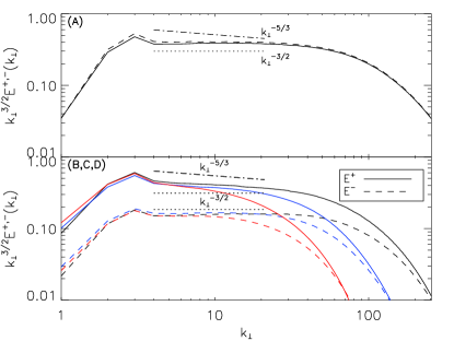
Equations (3) are evolved until a stationary state is reached, as determined by the time evolution of the total energy of the fluctuations, (see figure 2). A typical run produces over 200 snapshots; the large-scale dynamic time associated to the dominant large scale mode $k_{\perp}\sim 3$ is $(L_{\perp}/3)/u_{rms}\sim 2$.

Figure 2: Evolution of energy for imbalanced run. The outer-scale dynamic time is about $(L_{\perp}/3)/u_{rms}\sim 2$.

Since the background magnetic field must be strong, we choose $B_{0}=5$ in the $v_{rms}$ units, (see the discussion in (Mason et al., 2006)). Time is normalized to the Alfvén transit time $\tau_{0}=L_{\|}/v_{A}$, where $L_{\|}$ is the field-parallel box size. This time is equivalent to the perpendicular transit time $L_{\perp}/v_{rms}$ when $v_{rms}=1$. The Reynolds number is defined as $Re=v_{rms}(L_{\perp}/2\pi)/\nu$ and we have chosen the same value for the magnetic Reynolds number, $Rm={b}_{rms}(L_{\perp}/2\pi)/\eta$, denoting both by $R$ in (3). In each run, the average is performed over about 100 large-scale-eddy turnover times. The results are presented in Fig. (3).

Run	Resolution	$Re$	$\nu=\eta$	$L_{\|}/L_{\perp}$	$\sigma_{c}$
A	$512^{2}\times 256$	2400	$4.2\times 10^{-4}$	5	0
B	$256^{3}$	900	$1.1\times 10^{-3}$	10	0.6
C	$512^{2}\times 256$	2200	$4.6\times 10^{-4}$	10	0.6
D	$1024^{2}\times 256$	5600	$1.8\times 10^{-4}$	10	0.6

Table 1: Summary of simulations of strong balanced turbulence (A) and strong imbalanced turbulence (B, C, D).

Table 1 summarizes five representative simulations that incorporate all the aspects discussed in section III. Run A correspond to balanced turbulence, that is, $\sigma_{c}=0$. In runs labeled B, C and D, cross helicity is injected at the forcing scale in such a way that $\sigma_{c}$ reaches a steady state of $\sim 0.6$. We use a short time-correlated forcing, which is on average $1/20^{th}$ of the Alfvén time of the excited modes, so that the energy injection rates for both $\mathbf{z}^{+}$ and $\mathbf{z}^{-}$ only depend on the variance of the imposed forcing, which is controlled in our simulations. In the imbalanced case, field-parallel box size is optimized to reach the critical balance at the large scales. Except for the Reynolds numbers, simulations B, C, and D have the exact same parameters including the energy injection rates, $\epsilon^{+}$ and $\epsilon^{-}$.

Figure 3: Spectra of the Elsässer fields in numerical simulations of strong MHD turbulence. Top two frames: balanced turbulence (run A); bottom frame: imbalanced turbulence (runs B(red), C(blue) and D(black)).

The field-perpendicular energy spectrum is obtained by averaging the angle-integrated Fourier spectrum,

$$E(k_{\perp})=0.5\langle|{\bf v}({\bf k_{\perp}})|^{2}\rangle k_{\perp}+0.5\langle|{\bf b}({\bf k_{\perp}})|^{2}\rangle k_{\perp},$$ (7)

over field-perpendicular planes in all snapshots. Figure 3 shows the field-perpendicular energy spectra for each run.

Our numerical setup offers significant advantages over full MHD simulations, and can be already seen in simulations of balanced turbulence, top frame in Fig. (3), run A. The energy spectra approach $E^{\pm}(k_{\perp})\propto k_{\perp}^{-3/2}$, in good agreement with earlier numerical findings (e.g., Maron and Goldreich, 2001; Haugen et al., 2003; Müller and Grappin, 2005; Mason et al., 2006), but requiring considerably less computational cost and producing slightly larger inertial intervals. Our most significant results are obtained for the imbalanced case. The bottom frame of Fig. 3 shows the spectra for three different Reynolds numbers (runs B, C, D). It is observed that the spectra $E^{\pm}$ are pinned at the dissipation scales, which supports the phenomenological predictions by Grappin et al. (1983); Galtier et al. (2000); Lithwick and Goldreich (2003); Chandran (2008). We also find that the large-scale parts of the both spectra are practically insensitive to the Reynolds numbers. These two important properties imply that as the Re numbers are further increased, the $E^{\pm}$ spectra must become progressively more parallel in the inertial interval. This is indeed seen in our numerical simulations (B, C, D). Our numerical simulations indicate that both spectra approach the universal scaling of strong MHD turbulence $E^{\pm}(k_{\perp})\propto k_{\perp}^{-3/2}$, while they have essentially different amplitudes and correspond to essentially different energy fluxes.

V Phenomenological modeling

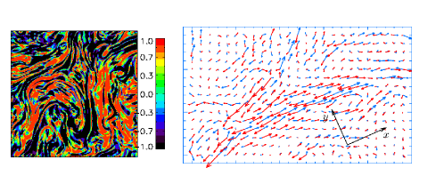
In this section we propose an explanation for the observed spectra. In the case of balanced MHD turbulence, our explanation of the $k_{\perp}^{-3/2}$ energy spectrum relies on the phenomenon of scale-dependent dynamic alignment, see Boldyrev (2006); Mason et al. (2008). (General details on dynamic alignment in MHD turbulence can be found in, e.g., Matthaeus and Montgomery (1984); Biskamp (2003)). Consider the eddy shown to the right of Fig. 4, obtained from simulations. In this eddy fluctuations are aligned within the small angle $\theta_{\lambda}$ along $x$, while their directions and magnitudes change in an almost perpendicular direction, along $y$. In the case of strong balanced turbulence, the nonlinear interaction in such an eddy is then reduced by a factor $\theta_{\lambda}$ for both $z^{+}$ and $z^{-}$ fields, and the corresponding nonlinear interaction time is estimated as $\tau_{\lambda}\sim 1/({\bf z}^{\pm}_{\lambda}\cdot{\bf k}_{\perp})\sim 1/(z^{\pm}_{\lambda}k_{\perp}\theta_{\lambda})$. The scaling of the fluctuating fields is then found from the requirement of constant energy fluxes: $(z_{\lambda}^{\pm})^{2}/\tau_{\lambda}={\rm const}$. One can argue (Boldyrev, 2006; Mason et al., 2006, 2008) that the alignment angle decreases with scale as $\theta_{\lambda}\propto\lambda^{1/4}$, in which case the field-perpendicular energy spectrum is $E(k_{\perp})\propto k_{\perp}^{-3/2}$.

Figure 4: Left: Cosine of the alignment angle between ${\bf v}_{\lambda}$ and ${\bf b}_{\lambda}$ fluctuations in the guide-field perpendicular plane at scale $\lambda=L_{\perp}/12$ in Run A. Right: A correlated region of (counter-)aligned magnetic and velocity fluctuations (red and blue vectors) at scale $\lambda=L_{\perp}/12$, in a plane perpendicular to the strong guide field, in run A. The fluctuations are aligned predominantly in the $x$ direction while their directions and amplitudes change predominantly in the $y$ direction.

Figure 5: Sketch of dynamic alignment of magnetic and velocity fluctuations in a turbulent eddy.

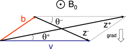
It turns out that the imbalanced simulations of previous section can also be explained within the framework of the scale-dependent dynamic alignment Perez and Boldyrev (2009, 2010). Let us assume that the alignment is present in the imbalanced case. Since the fields amplitudes $z^{+}$ and $z^{-}$ are now essentially different, the alignment angles are different as well; we denote them $\theta_{\lambda}^{+}$ and $\theta_{\lambda}^{-}$, see Fig. 5. These angles obey the important geometric constraint: $\theta_{\lambda}^{+}z_{\lambda}^{+}\sim\theta_{\lambda}^{-}z_{\lambda}^{-}$, as is clear from Fig. 5. The depletion of nonlinear interaction Kraichnan and Panda (1988); Servidio et al. (2008) is therefore different for $z^{+}$ and $z^{-}$ fields, which makes their nonlinear interaction times, $\tau^{\mp}_{\lambda}\sim 1/(z^{\pm}_{\lambda}k_{\perp}\theta^{\pm}_{\lambda})$, the same. The requirement of constant energy fluxes $(z_{\lambda}^{\pm})^{2}/\tau^{\pm}_{\lambda}\sim\epsilon^{\pm}={\rm const}$ then ensures that $z_{\lambda}^{+}/z_{\lambda}^{-}\sim\sqrt{\epsilon^{+}/\epsilon^{-}}$, so both fields should have the same scaling, although different amplitudes. We also note that the Reynolds numbers that take into account the depletion of nonlinear interaction are the same for both fields, $Re_{\lambda}^{\pm}\sim\lambda z_{\lambda}^{\mp}\theta_{\lambda}^{\mp}/\nu$, and they are reduced approximately by the factor $\gamma=z^{+}/z^{-}$ with respect to the formal Reynolds number $Re_{\lambda}=\lambda v_{\lambda}/\nu$.

We note that the above relations of the kind $z_{\lambda}^{+}/z_{\lambda}^{-}\sim\sqrt{\epsilon^{+}/\epsilon^{-}}$ hold locally for a particular domain, with given (positive or negative) alignment, while MHD turbulence consists of both positively and negatively aligned domains of various strengths. Since $E^{+}$ and $\epsilon^{+}$ are concentrated mostly in positively aligned domains, while $E^{-}$ and $\epsilon^{-}$ in negatively aligned ones, the quantities $\langle z^{\pm}_{\lambda}\rangle$ and $\langle\epsilon^{\pm}\rangle$ averaged over the global system should not a priori satisfy the same relations. The difference between the local and global quantities in MHD turbulence should be taken into account when one designs numerical tests.

Recently, Beresnyak & Lazarian Beresnyak and Lazarian (2008, 2009) attempted to test the effects of the dynamic alignment in imbalanced turbulence by measuring the relations among global quantities $\langle z^{\pm}_{\lambda}\rangle$ and $\langle\epsilon^{\pm}\rangle$. They did not observe the local scaling relations and concluded that the dynamic alignment proposed in Perez and Boldyrev (2009, 2010) is absent. According to the explanation given above, such a conclusion is incorrect. The relations between the global quantities should depend on the details of the distribution of positive and negative domains in the turbulent system, see the discussion in Podesta and Bhattacharjee . For our present purposes we simply need the fact that if each domain has the same scaling of the fluctuating fields, the fields averaged over the whole turbulent system will have the same scaling as well.

VI Discussion.

We have presented a detailed numerical setup based on the Reduced MHD model (RMHD), and results from high resolution simulations of balanced and imbalanced MHD turbulence in steady state. We have used this numerical set up to address currently existing controversies regarding the spectra of imbalanced MHD turbulence. The simulations are consistent with the theories and observations predicting same scaling for both Elsässer fields  (Beresnyak and Lazarian, 2008; Lithwick et al., 2007; Perez and Boldyrev, 2009; Podesta and Bhattacharjee, ) and less consistent with the models predicting different scalings for $E^{\pm}$, (e.g., Chandran, 2008). The measured scaling exponent in the simulations is close to the $-3/2$ supported by phenomenological models based on dynamic alignment Perez and Boldyrev (2009); Podesta and Bhattacharjee . The analysis of our simulation results may also explain somewhat puzzling numerical findings by Beresnyak and Lazarian (2008, 2009), who report different spectra for the $E^{\pm}$ Elsässer fields, and the intersection of the spectra rather than pinning at the dissipation scale. According to our results, the explanation might lie in the fact that in these simulations the imbalance was typically high, up to $\gamma^{2}=(z^{+})^{2}/(z^{-})^{2}\sim 1000$, and, therefore, the universal regime of imbalanced MHD turbulence was not reached, see our analysis in section III.5.

The phenomenology of scale-dependent dynamic alignment can be applied to explain the observed spectra. In this phenomenology, the configuration space splits into eddies (domains) with highly aligned and anti-aligned magnetic and velocity fluctuations, where nonlinear interactions are reduced, as in left panel of Fig. 4. Even when the turbulence is balanced overall it still can be imbalanced locally, creating domains of positive and negative cross-helicity. In each of these regions the picture of imbalanced turbulence presented above applies. When averaged over all the regions, the spectra of balanced turbulence are reproduced.

This work was supported by the U.S. DOE Junior Faculty grant DE-FG02-07ER54932, by the DOE grant DE-SC0001794, and by the NSF Center for Magnetic Self-Organization in Laboratory and Astrophysical Plasmas at the University of Wisconsin-Madison. High Performance Computing resources were provided by the Texas Advanced Computing Center (TACC) at the University of Texas at Austin under the NSF-Teragrid Project TG-PHY070027T.

References

- Coleman (1966) P. J. Coleman, Phys. Rev. Lett. 17, 207 (1966).
- Coleman (1968) P. J. Coleman, Jr., Astrophys. J. 153, 371 (1968).
- Belcher and Davis (1971) J. W. Belcher and L. Davis, Jr., J. Geophys. Res. 76, 3534 (1971).
- Marsch (1991) E. Marsch, in Physics of the inner heliosphere 2. Particles, waves and turbulence, edited by S. R. and E. Marsch (Springer, Berlin, 1991), pp. 159–241.
- Goldstein et al. (1995) M. L. Goldstein, D. A. Roberts, and W. H. Matthaeus, Annu. Rev. Astron. Astrophys. 33, 283 (1995).
- Armstrong et al. (1995) J. W. Armstrong, B. J. Rickett, and S. R. Spangler, Astrophys. J. 443, 209 (1995).
- Lithwick and Goldreich (2001) Y. Lithwick and P. Goldreich, Astrophys. J. 562, 279 (2001).
- Kolmogorov (1941) A. Kolmogorov, Akademiia Nauk SSSR Doklady 30, 301 (1941). A. N. Kolmogorov, Royal Society of London Proceedings Series A 434, 9 (1991).
- Obukhov (1941) A. Obukhov, Akademiia Nauk SSSR Doklady 32, 22 (1941).
- Iroshnikov (1963) P. S. Iroshnikov, AZh 40, 742 (1963).
- Kraichnan (1965) R. H. Kraichnan, Physics of Fluids 8, 1385 (1965).
- Montgomery and Turner (1981) D. Montgomery and L. Turner, Physics of Fluids 24, 825 (1981).
- Shebalin et al. (1983) J. V. Shebalin, W. H. Matthaeus, and D. Montgomery, Journal of Plasma Physics 29, 525 (1983).
- Goldreich and Sridhar (1995) P. Goldreich and S. Sridhar, Astrophys. J. 438, 763 (1995).
- Cho and Vishniac (2000) J. Cho and E. T. Vishniac, Astrophys. J. 539, 273 (2000).
- Maron and Goldreich (2001) J. Maron and P. Goldreich, Astrophys. J. 554, 1175 (2001).
- Haugen et al. (2003) N. E. L. Haugen, A. Brandenburg, and W. Dobler, Astrophys. J. 597, L141 (2003).
- Biskamp (2003) D. Biskamp, Magnetohydrodynamic Turbulence (Cambridge University Press, Cambridge, UK, 2003).
- Müller and Grappin (2005) W.-C. Müller and R. Grappin, Phys. Rev. Lett. 95, 114502 (2005).
- Mason et al. (2006) J. Mason, F. Cattaneo, and S. Boldyrev, Phys. Rev. Lett. 97, 255002 (2006).
- Mason et al. (2008) J. Mason, F. Cattaneo, and S. Boldyrev, Phys. Rev. E 77, 036403 (2008).
- Mininni and Pouquet (2007) P. D. Mininni and A. Pouquet, Phys. Rev. Lett. 99, 254502 (2007).
- Beresnyak and Lazarian (2008) A. Beresnyak and A. Lazarian, Astrophys. J. 682, 1070 (2008).
- Perez and Boldyrev (2008) J. C. Perez and S. Boldyrev, Astrophys. J. 672, L61 (2008).
- Perez and Boldyrev (2009) J. C. Perez and S. Boldyrev, Phys. Rev. Lett. 102, 025003 (2009).
- Lithwick et al. (2007) Y. Lithwick, P. Goldreich, and S. Sridhar, Astrophys. J. 655, 269 (2007).
- Chandran (2008) B. D. G. Chandran, Astrophys. J. 685, 646 (2008).
- Beresnyak and Lazarian (2009) A. Beresnyak and A. Lazarian, Astrophys. J. 702, 460 (2009).
- (29) J. J. Podesta and A. Bhattacharjee, submitted to Phys. of Plasmas (ArXiv e-print: 0903.5041).
- Perez and Boldyrev (2010) J. C. Perez and S. Boldyrev, The Astrophysical Journal Letters 710, L63 (2010).
- Elsasser (1956) W. M. Elsasser, Reviews of Modern Physics 28, 135 (1956).
- Kadomtsev and Pogutse (1974) B. B. Kadomtsev and O. P. Pogutse, JETP 38, 283 (1974).
- Strauss (1976) H. R. Strauss, Physics of Fluids 19, 134 (1976).
- Oughton et al. (2004) S. Oughton, P. Dmitruk, and W. H. Matthaeus, Physics of Plasmas 11, 2214 (2004).
- Borue and Orszag (1995) V. Borue and S. A. Orszag, Europhysics Letters 29, 687 (1995).
- Gotoh et al. (2002) T. Gotoh, D. Fukayama, and T. Nakano, Physics of Fluids 14, 1065 (2002).
- Alexakis et al. (2005) A. Alexakis, P. D. Mininni, and A. Pouquet, Phys. Rev. E 72, 046301 (2005).
- Alexakis et al. (2007) A. Alexakis, B. Bigot, H. Politano, and S. Galtier, Phys. Rev. E 76, 056313 (2007).
- Carati et al. (2006) D. Carati, O. Debliquy, B. Knaepen, B. Teaca, and M. Verma, Journal of Turbulence 7, 51 (2006).
- Yousef et al. (2007) T. A. Yousef, F. Rincon, and A. A. Schekochihin, Journal of Fluid Mechanics 575, 111 (2007).
- Aluie and Eyink (2010) H. Aluie and G. L. Eyink, Physical Review Letters 104, 081101 (2010).
- Grappin et al. (1983) R. Grappin, J. Leorat, and A. Pouquet, Astron. Astrophys. 126, 51 (1983).
- Galtier et al. (2000) S. Galtier, S. V. Nazarenko, A. C. Newell, and A. Pouquet, Journal of Plasma Physics 63, 447 (2000).
- Lithwick and Goldreich (2003) Y. Lithwick and P. Goldreich, Astrophys. J. 582, 1220 (2003).
- Boldyrev (2006) S. Boldyrev, Phys. Rev. Lett. 96, 115002 (2006).
- Matthaeus and Montgomery (1984) W. H. Matthaeus and D. Montgomery, in Statistical Physics and Chaos in Fusion Plasmas, edited by C. W. Horton Jr. & L. E. Reichl (Proceedings of the Workshop held at the University of Texas at Austin, December, 1982, 1984), p. 285.
- Kraichnan and Panda (1988) R. H. Kraichnan and R. Panda, Physics of Fluids 31, 2395 (1988).
- Servidio et al. (2008) S. Servidio, W. H. Matthaeus, and P. Dmitruk, Phys. Rev. Lett. 100, 095005 (2008).