Degeneracy measures for the algebraic classification of numerical spacetimes

Abstract

We study the issue of algebraic classification of the Weyl curvature tensor, with a particular focus on numerical relativity simulations. The spacetimes of interest in this context, binary black hole mergers, and the ringdowns that follow them, present subtleties in that they are generically, strictly speaking, Type I, but in many regions approximately, in some sense, Type D. To provide meaning to any claims of “approximate” Petrov class, one must define a measure of degeneracy on the space of null rays at a point. We will investigate such a measure, used recently to argue that certain binary black hole merger simulations ring down to the Kerr geometry, after hanging up for some time in Petrov Type II. In particular, we argue that this hangup in Petrov Type II is an artefact of the particular measure being used, and that a geometrically better-motivated measure shows a black hole merger produced by our group settling directly to Petrov Type D.

I Introduction:

The marvelous improvements in the technology of numerical relativity in recent years present opportunities for revolutionizing our understanding of the classical gravitational field. In the past, much of this understanding has come from studying solutions with extreme symmetry, and perturbations of such solutions. However, with the help of numerical methods, truly generic simulations, particularly of multiple black hole systems, can now be carried out in full general relativity.

While this work is undertaken, one must keep in mind the fundamental nature of general relativity and its solutions. In particular, the general covariance of the theory is not naturally reflected in the numerical context, where gauge fixing is fundamentally required in the form of coordinate and tetrad choices. In practice, such gauge choices are tailored to numerical convenience (or necessity), rather than to physical relevance. Such a simple task as checking that a black hole merger settles down to a Kerr geometry can be clouded by the arbitrariness of the simulation coordinates.

One way of dealing with these ambiguities would be to apply coordinate transformations to numerical simulations a posteriori to represent these spacetimes in physically preferable coordinates, if they exist. If one needs to map all quantities to an entirely new coordinate grid, then some accuracy would presumably be lost to the interpolation process, especially if changes of the time function require interpolation in time. More important, however, is the difficulty of fixing physically preferred coordinate systems in strongly dynamical and nonsymmetric spacetimes at all.

Another, perhaps complimentary, approach is to focus physical analysis on partially (or if possible, totally) gauge invariant quantities. For example, a major tool in the analysis (and construction) of exact solutions in general relativity is the algebraic classification system of Petrov and Pirani Petrov (2000); Pirani (1957); Stephani et al. (2003), in which the Weyl tensor at any given point in spacetime is classified according to the algebraic properties of its associated eigenbivector problem:

$${C_{ab}}^{cd}X_{cd}=\Lambda X_{ab}.$$ (1)

Another view of this classification system, with a more geometrical flavor, was expounded particularly by Bel Bel (1962) and Penrose Penrose (1960). In this approach one classifies the Weyl tensor in terms of the degeneracy of the so-called principal null directions, null vectors defined up to scale by the equation:

$$k^{e}k^{f}k_{[a}C_{b]ef[c}k_{d]}=0.$$ (2)

One can show (most easily in spinor language) that this equation is always satisfied by exactly four null rays, counting multiplicities. If all four of these null directions are distinct, the spacetime is said to be algebraically general or Type I at that point in spacetime. If two of them coincide, the spacetime is said to be Type II there. If three, Type III. If all four principal null directions coincide, the spacetime is said to be Type N, or null, in analogy with the pure radiation fields of vacuum electrodynamics. If the principal null directions coincide in two distinct pairs, then the spacetime is said to be Type D. The Kerr and Schwarzschild geometries are famous examples of globally Type D spacetimes, so in some sense, one may hope to infer that a spacetime is “settling down to an approximate Kerr geometry” if its Petrov type “settles down” to Type D (assuming that one has ruled out other, non-Kerr, Type D spacetimes).

This line of reasoning was taken up in a paper by Campanelli, Lousto, and Zlochower Campanelli et al. (2009). The central tool in their approach is a certain complex polynomial equation:

$$\Psi_{4}\lambda^{4}+4\Psi_{3}\lambda^{3}+6\Psi_{2}\lambda^{2}+4\Psi_{1}\lambda+\Psi_{0}=0,$$ (3)

the degeneracy of whose roots is known to correspond to the degeneracy of the principal null directions (assuming that $\Psi_{4}$ is nonzero). The coefficients $\Psi_{i}$ of this polynomial are the so-called Weyl scalars, components (defined in Eq. (9) below) of the Weyl tensor in a given Newman-Penrose null tetrad. If $\Psi_{4}$ is nonzero, then the fundamental theorem of algebra ensures that the polynomial has exactly four complex roots, counting multiplicities.

Once the four roots $\lambda_{i}$ have been computed for Eq. (3) at any given point, then one can also compute six distinct positive-definite root differences:

$$\Delta_{ij}:=|\lambda_{i}-\lambda_{j}|.$$ (4)

If two of these root differences vanish and the other four are nonzero, meaning that the four roots coincide in two distinct pairs, then the spacetime is Type D at that point. In Ref. Campanelli et al. (2009) Campanelli et al. took the next logical step: interpreting the two smallest $\Delta_{ij}$ values as measures of the “nearness” of an algebraically general (in that case, numerical) spacetime to Petrov Type D. While this is a reasonable interpretation of $\Delta_{ij}$ and we will not suggest any fundamental modification to this approach of defining approximate algebraic speciality, there are important subtleties in this interpretation, not fully explored in Ref. Campanelli et al. (2009). These subtleties relate to the geometrical meaning of $\Delta_{ij}$ and its behavior under tetrad transformations. The main purpose of this paper is to explore these subtleties, present an alternative degeneracy measure that avoids certain blowups that are intricately related to the choice of tetrad (and should therefore not be considered physically relevant), and apply both degeneracy measures to a numerical simulation from the SpEC code SpEC . In the process we will also investigate an interesting conclusion from Ref. Campanelli et al. (2009): that in the ringdown of a binary black hole merger to Kerr, the spacetime approaches Petrov Type II very quickly, and Type D much later. We will argue that this conclusion is due essentially to a coordinate singularity on the space of null rays, and the fact that the tetrad used in Ref. Campanelli et al. (2009) was much better suited to representing the degeneracy of one pair of principal null directions than the other pair, when the degeneracy measure $\Delta_{ij}$ is used. The alternate degeneracy measure that we will introduce, $\Theta_{ij}$ defined in Eq. (45) below, shows both pairs of principal null directions approaching degeneracy at the same rate.

Though much of the discussion in this paper centers upon the behavior of these measures of degeneracy under tetrad transformations, we will unfortunately not be able to provide a measure of nearness to Petrov Type D that is fundamentally any more invariant than $\Delta_{ij}$. This is because no such measure appears to exist. Geometrically this fact can be understood in terms of the nonexistence of a boost-invariant geometry on the space of null rays in Minkowski space, an issue referred to physically as the “relativistic aberration of starlight.” This viewpoint is explored in more detail in Section IV below.

The issue can also be understood at the algebraic level, as in Petrov’s original construction. The problem shown in Eq. (1) can be written more compactly if one works in the three-complex-dimensional space of anti-self-dual bivectors rather than in the six-real-dimensional space of real bivectors. In this space, the eigenbivector problem can be written as:

$${W_{ab}}^{cd}Z_{cd}=\Lambda Z_{ab},$$ (5)

where $W_{abcd}:=C_{abcd}+i\hskip 2.84526pt{}^{\star}C_{abcd}$, ${}^{\star}Z_{ab}=-iZ_{ab}$, and $\Lambda$ is a complex number. Because this is a three-dimensional problem one can expect three possible values for $\Lambda$, though the fact that the Weyl tensor is tracefree implies that these three eigenvalues must sum to zero. The degeneracy of the eigenvalues and the completeness of the corresponding eigenspaces determine the classification of the Weyl tensor at the point under consideration. If all three eigenvalues are distinct then the spacetime is algebraically general. If two roots coincide, then the spacetime is either Type II or Type D. If all three coincide (and therefore vanish, as they must sum to zero) then the spacetime is either Type III, Type N, or conformally flat. The eigenvalues are geometrically defined at each point in spacetime, independent of the vector basis used to represent the eigenproblem. The differences between these eigenvalues can therefore be used to construct invariant measures of the approach to algebraic speciality. For example, the absolute value of the difference between the two nearest eigenvalues can be thought of as such an invariant measure. Unfortunately this measure isn’t very specific: it vanishes for Petrov Types II, D, III, and N. The latter pair can be distinguished from the former pair by the fact that all three eigenvalues vanish in Type III and Type N, but distinguishing Type II from Type D, or Type III from Type N, requires more information than just the eigenvalues.

If two of the eigenvalues in Eq. (5) coincide, so that the eigenvalues can be written as $\{\Lambda,\Lambda,-2\Lambda\}$, then the distinction between Petrov Type II and Type D can be made by the following quantity:

$${T^{ab}}_{cd}:=({W^{ab}}_{ef}-\Lambda I^{ab}_{ef})({W^{ef}}_{cd}+2\Lambda I^{ef}_{cd}),$$ (6)

where $I^{ab}_{cd}$ is the identity operator on the space of anti-self-dual bivectors. The object ${T^{ab}}_{cd}$ vanishes in Type D, but not in Type II Stephani et al. (2003). The difficulty with using this as a measure of nearness to Petrov Type D is that it is a tensorial object, and its components are, by definition, basis-dependent. In order to collapse this object to a single number for each point in spacetime, one might hope to construct a positive-definite tensor norm:

$$Q:=m_{ae}\hskip 2.84526ptm_{bf}\hskip 2.84526ptm^{cg}\hskip 2.84526ptm^{dh}\hskip 2.84526pt{T^{ab}}_{cd}\hskip 2.84526pt{\overline{T}^{ef}}{}_{gh},$$ (7)

where $m_{ab}$ is a positive-definite inner product on spacetime. Unfortunately, the only inner product that one naturally has available on spacetime is the indefinite spacetime metric. If a timelike “observer” is introduced, with unit tangent vector $u^{a}$, then one can construct a positive definite inner product as:

$$m_{ab}:=g_{ab}+2u_{a}u_{b},$$ (8)

but then the quantity $Q$ is not strictly a scalar, as its definition is dependent on the extra structure of this observer.

Though the language is very different in the geometric approach involving principal null directions, we will find in Section IV that the ambiguity in defining a measure of “nearness” to Petrov Type D is in that context essentially the same as here, requiring the choice of a timelike observer at every point in spacetime. While this state of affairs seems to endanger any attempt at defining the nearness to any specific Petrov class, there are some cases where a well-defined fleet of observers can be chosen. In particular, in any stationary spacetime, one can choose the stationary observers. In cases such as the ringdown to Kerr geometry, one can expect an “approximate” stationarity to be approached at late times, again providing a preferred class of observers at least during the late ringdown. A major practical goal of this paper will be to study this ringdown process, as in Ref. Campanelli et al. (2009). In particular, we will argue that the degeneracy measure $\Delta_{ij}$ that was used in Ref. Campanelli et al. (2009) is in some sense adapted to a null observer that happened in that case to be nearly aligned with one of the nearly degenerate pairs of principal null directions, making this pair of null directions seem much more degenerate, and the other, much less. This causes the appearance of a holdup in Petrov Type II before the spacetime geometry falls to Type D.

The structure of this paper is as follows: in Sec. II we will investigate the ambiguity of the measure $\Delta_{ij}$ under tetrad rotations, particularly those that leave the timelike tetrad leg fixed. In Sec. III we will emphasize the fact that a tetrad well-suited to gravitational wave extraction, in particular the quasi-Kinnersley tetrad Nerozzi et al. (2005), may be particularly ill-suited to measuring the nearness to Petrov Type D using $\Delta_{ij}$. In Sec. IV we will describe the geometry underlying $\Delta_{ij}$ in spinorial language, and in the process motivate a modification that is much better suited to situations such as the ringdown to Kerr geometry. In Sec. V we will present numerical results applying these degeneracy measures to a binary black hole merger simulation, demonstrating in detail the approach to Petrov Type D. Finally in Sec. VI we conclude with further discussion of the subtleties that have been addressed, and those that remain.

II Tetrad dependence

The method put forth in Ref. Campanelli et al. (2009) to define nearness to a Petrov class begins with the polynomial in Eq. (3), whose coefficients are components of the Weyl tensor in a Newman-Penrose tetrad Newman and Penrose (1962):

$$\Psi_{0} := C_{abcd}\ell^{a}m^{b}\ell^{c}m^{d},$$ (9a)

$$\Psi_{1} := C_{abcd}\ell^{a}n^{b}\ell^{c}m^{d},$$ (9b)

$$\Psi_{2} := \frac{1}{2}C_{abcd}\left(\ell^{a}n^{b}\ell^{c}n^{d}-\ell^{a}n^{b}m^{c}\overline{m}^{d}\right),$$ (9c)

$$\Psi_{3} := C_{abcd}n^{a}\ell^{b}n^{c}\overline{m}^{d},$$ (9d)

$$\Psi_{4} := C_{abcd}n^{a}\overline{m}^{b}n^{c}\overline{m}^{d}.$$ (9e)

The tetrad $\{\ell^{a},n^{a},m^{a},\overline{m}^{a}\}$ is made up of two future-directed real null vectors $\ell^{a}$ and $n^{a}$ and two complex conjugate null vectors $m^{a}$ and $\overline{m}^{a}$ with spacelike real and imaginary parts. These vectors are normalized by the conditions:

$$\ell_{a}n^{a} = -1,$$ (10)

$$m_{a}\overline{m}^{a} = 1,$$ (11)

$$\ell_{a}m^{a}=n_{a}m^{a} = 0.$$ (12)

These normalization conditions are preserved by three types of tetrad transformations which, taken together, are equivalent to the proper Lorentz group. First, there are the “null rotations about $\ell^{a}$,” sometimes referred to as the “Type I” transformations:

$$\ell^{a} \mapsto \ell^{a},$$ (13a)

$$m^{a} \mapsto m^{a}+a\ell^{a},$$ (13b)

$$\overline{m}^{a} \mapsto \overline{m}^{a}+\overline{a}\ell^{a},$$ (13c)

$$n^{a} \mapsto n^{a}+\overline{a}m^{a}+a\overline{m}^{a}+a\overline{a}\ell^{a},$$ (13d)

where $a$ is a complex number, and can vary over spacetime. Second, there are the null rotations about $n^{a}$, sometimes referred to as “Type II” transformations:

$$\ell^{a} \mapsto \ell^{a}+\overline{b}m^{a}+b\overline{m}^{a}+b\overline{b}n^{a},$$ (14a)

$$m^{a} \mapsto m^{a}+bn^{a},$$ (14b)

$$\overline{m}^{a} \mapsto \overline{m}^{a}+\overline{b}n^{a},$$ (14c)

$$n^{a} \mapsto n^{a},$$ (14d)

for complex $b$. Third, there are the “spin-boost” transformations, sometimes referred to as the “Type III” transformations:

$$\ell^{a} \mapsto |c|^{2}\ell^{a},$$ (15a)

$$m^{a} \mapsto e^{2i\arg(c)}m^{a},$$ (15b)

$$\overline{m}^{a} \mapsto e^{-2i\arg(c)}\overline{m}^{a},$$ (15c)

$$n^{a} \mapsto |c|^{-2}n^{a},$$ (15d)

for complex $c$.

These transformation laws for the tetrad imply transformation laws for the Weyl scalars. Under the null rotations about $\ell^{a}$, Eqs. (13), the Weyl scalars transform as:

$$\Psi_{0} \mapsto \Psi_{0},$$ (16a)

$$\Psi_{1} \mapsto \Psi_{1}+\overline{a}\Psi_{0},$$ (16b)

$$\Psi_{2} \mapsto \Psi_{2}+2\overline{a}\Psi_{1}+\overline{a}^{2}\Psi_{0},$$ (16c)

$$\Psi_{3} \mapsto \Psi_{3}+3\overline{a}\Psi_{2}+3\overline{a}^{2}\Psi_{1}+\overline{a}^{3}\Psi_{0},$$ (16d)

$$\Psi_{4} \mapsto \Psi_{4}+4\overline{a}\Psi_{3}+6\overline{a}^{2}\Psi_{2}+4\overline{a}^{3}\Psi_{1}+\overline{a}^{4}\Psi_{0}.$$ (16e)

Under null rotations about $n^{a}$, Eqs. (14), the Weyl scalars transform as:

$$\Psi_{0} \mapsto b^{4}\Psi_{4}+4b^{3}\Psi_{3}+6b^{2}\Psi_{2}+4b\Psi_{1}+\Psi_{0},$$ (17a)

$$\Psi_{1} \mapsto b^{3}\Psi_{4}+3b^{2}\Psi_{3}+3b\Psi_{2}+\Psi_{1},$$ (17b)

$$\Psi_{2} \mapsto b^{2}\Psi_{4}+2b\Psi_{3}+\Psi_{2},$$ (17c)

$$\Psi_{3} \mapsto b\Psi_{4}+\Psi_{3},$$ (17d)

$$\Psi_{4} \mapsto \Psi_{4}.$$ (17e)

Finally, under the spin boosts, Eqs. (15), the Weyl scalars simply rescale, as:

$$\Psi_{n}\mapsto c^{2(2-n)}\Psi_{n}.$$ (18)

The transformation laws for the coefficients of the polynomial in Eq. (3) imply transformation laws for the roots. It is straightforward to show that under the transformation in Eq. (16), the roots of the polynomial transform as:

$$\lambda\mapsto\frac{\lambda}{\overline{a}\lambda+1}.$$ (19)

Under transformations of the form (17), the roots transform as:

$$\lambda\mapsto\lambda+b.$$ (20)

Finally, under spin-boost transformations, Eq. (18), the roots transform as:

$$\lambda\mapsto c^{2}\lambda.$$ (21)

In Ref. Campanelli et al. (2009), nearness to Petrov Type D was mainly argued through the approach of the absolute values of root differences ($\Delta_{ij}$ as defined in Eq. (4)) to zero. While this quantity would indeed be expected to vanish when $\lambda_{i}$ and $\lambda_{j}$ constitute a degenerate root pair, if they are not exactly degenerate, then the foregoing discussion implies that this difference is not invariant under tetrad transformations. The transformation in Eq. (20) would leave $\Delta_{ij}$ unchanged, but that in Eq. (21) would directly rescale any given root difference (though the complex phase of $c$ would not appear in the absolute value), and transformations of the form (19) would change $\Delta_{ij}$ in a more complicated way. Arbitrary Lorentz transformations, given by arbitrary combinations of the above transformations, could alter $|\lambda_{i}-\lambda_{j}|$ in a very complicated manner.

To investigate the practical relevance of this tetrad ambiguity in the degeneracy measure $\Delta_{ij}$, let us consider a particular case of possible physical relevance that requires a combination of all three of the above tetrad transformations. Take the case where one has a particular timelike vector defined at a point in spacetime, for example a timelike Killing vector, or a kind of approximate Killing vector generating time translations in a spacetime that is approaching stationarity in some sense. Given a Newman-Penrose tetrad $\{\ell^{a},n^{a},m^{a},\overline{m}^{a}\}$, one can construct a standard orthonormal tetrad in the following way:

$$e_{0}^{a} := (\ell^{a}+n^{a})/\sqrt{2},$$ (22a)

$$e_{1}^{a} := \sqrt{2}\hskip 5.69054pt{\rm Re}\left[m^{a}\right],$$ (22b)

$$e_{2}^{a} := \sqrt{2}\hskip 5.69054pt{\rm Im}\left[m^{a}\right],$$ (22c)

$$e_{3}^{a} := (\ell^{a}-n^{a})/\sqrt{2}.$$ (22d)

Rotations of the tetrad legs in the $\vec{e}_{1}$–$\vec{e}_{2}$ plane are easily accomplished, through a simple spin-boost transformation with the parameter $c=e^{i\Phi/2}$. Such rotations also however leave the degeneracy measure $\Delta_{ij}$ unchanged. For a nontrivial test case, consider a rotation in the $\vec{e}_{1}$–$\vec{e}_{3}$ plane:

$$\vec{e}_{0}{}^{\prime} = \vec{e}_{0}$$ (23a)

$$\vec{e}_{1}{}^{\prime} = \cos(\Phi)\vec{e}_{1}-\sin(\Phi)\vec{e}_{3}$$ (23b)

$$\vec{e}_{2}{}^{\prime} = \vec{e}_{2}$$ (23c)

$$\vec{e}_{3}{}^{\prime} = \cos(\Phi)\vec{e}_{3}+\sin(\Phi)\vec{e}_{1}$$ (23d)

A straightforward calculation shows that such a transformation can be carried out by a sequence of the above transformations. First, one makes a null rotation about $\ell^{a}$, Eqs. (13), with parameter $a=-\tan(\Phi/2)$. Second, there is a null rotation about $n^{a}$, Eqs. (14), with parameter $b=(1/2)\sin(\Phi)$. The final step is a spin boost, Eqs. (15), with parameter $c=\sec(\Phi/2)$. In this particular case, all three parameters are real. Composing the transformation laws for the roots, Eqs. (19) – (21), with these parameters, the resulting transformation law is:

$$\lambda^{\prime}=\frac{\lambda\cos(\Phi/2)-\sin(\Phi/2)}{\lambda\sin(\Phi/2)+\cos(\Phi/2)}.$$ (24)

If we express $\lambda$ as a ratio of two complex numbers, $\lambda=\xi/\eta$, then Eq. (24) takes a very simple matrix form:

$$\begin{pmatrix}\xi^{\prime}\\ \eta^{\prime}\end{pmatrix}=\begin{bmatrix}\cos(\Phi/2)&-\sin(\Phi/2)\\ \sin(\Phi/2)&\cos(\Phi/2)\end{bmatrix}\begin{pmatrix}\xi\\ \eta\end{pmatrix}.$$ (25)

The general form of this matrix, for arbitrary reorientations using three Euler angles, is given in Eq. (1.2.34) of Ref. Penrose and Rindler (1987). The $SL(2,\mathbb{C})$ form of this transformation suggests a spinorial interpretation of $\lambda$, a point to which we will return in Sec. IV.

For now let us consider the behavior of the degeneracy measure $\Delta_{ij}$ under these spatial rotations. For concreteness, consider the case where the four roots of Eq. (3) are $\lambda_{1}=.005+.047i$, $\lambda_{2}=.005+.05i$, $\lambda_{3}=-5+15i$, and $\lambda_{4}=-5+15.5i$. These values are chosen to very roughly mirror the late-term values seen in Fig. 8 of Ref. Campanelli et al. (2009), with degeneracies roughly similar to those seen in Figs. 3 and 4 of that paper. The values estimated here are extremely rough, and should not be taken as having any quantitative importance, but merely as tools for illustrating the qualitative features of the transformation law in Eq. (24). So long as one pair of nearly-degenerate roots is larger, by a few orders of magnitude, than the other pair, the qualitative behavior that we will describe seems roughly the same regardless of the particular choice of roots.

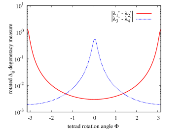
Figure 1: Behavior of the degeneracy measure $\Delta_{ij}$ under the tetrad rotation in Eq.(23) for a particular (though essentially arbitrary) choice of roots, stated in the text. Under a rotation through 180 degrees, the root pair that originally seemed more degenerate becomes less degenerate, and the pair that originally seemed less degenerate becomes more degenerate.

The degeneracy measure $\Delta_{ij}$ for the two most nearly degenerate root pairs, under rotation of the $\vec{e}_{1}$–$\vec{e}_{3}$ plane, is shown in Fig. 1. If the tetrad’s spatial legs were rotated through about ninety degrees, then both root pairs would appear equally close to degeneracy. If the tetrad were rotated through 180 degrees, then the root pair that originally appeared closer to degeneracy would begin to seem farther away from it, and the one that originally seemed less degenerate would seem more so.

This variation in the degeneracy measure can be interpreted as a coordinate effect. The quantity $\lambda$ has no inherent geometrical meaning without a particular reference tetrad. It is essentially a coordinate on the space of null rays at a point in spacetime. This space of null rays is topologically a two-dimensional sphere, as can be demonstrated by cutting a future null cone with a spacelike hyperplane, such as the $t=1$ plane in Minkowski space. A two-sphere cannot be covered smoothly with a single coordinate patch. If the quantity $\lambda$ is taken as a (complex) coordinate labeling all the null rays at a point, then there must be a coordinate singularity somewhere, near which coordinate distances are particularly ill-suited to representing the true geometry that may be defined on the manifold. We will study this issue in more detail in Sec. IV. For now we simply note that the locations of the sharp peaks in Fig. 1 seem to imply that such a coordinate singularity may have a particularly strong effect in the original, unrotated tetrad. The following section gives an extreme example of this effect.

III The quasi-Kinnersley tetrad:

It appears from the results of the previous section that a tetrad that seems reasonable for purposes of wave extraction can be particularly ill-suited to the problem of defining nearness to a Petrov class. To investigate this point in more detail, here we consider a special family of tetrads designed especially for wave extraction.

Consider an algebraically general spacetime (eventually we will allow this spacetime to “asymptote” toward Petrov Type D, but we will consider it always to be, strictly speaking, Type I). As described in Ref. Nerozzi et al. (2005), at any point where the Weyl tensor is Type I, there are precisely three distinct families of tetrads in which two particular Weyl scalars vanish, $\Psi_{1}=\Psi_{3}=0$ (they each amount to families of tetrads, rather than three particular tetrads, because this condition is preserved by the spin-boost freedom). A particular tetrad field, chosen from these three families to coincide with the conventional Kinnersley tetrad near infinity, is often referred to as a quasi-Kinnersley tetrad. The usual purpose of such a tetrad is to aid in gravitational wave extraction, where the relative uniqueness of the tetrad provides a preferred reference frame in which to define gravitational radiation. Such a tetrad also simplifies the polynomial in Eq. (3):

$$\Psi_{4}\lambda^{4}+6\Psi_{2}\lambda^{2}+\Psi_{0}=0.$$ (26)

If, as we are assuming, the spacetime is strictly Type I, and not a more special algebraic type, then $\Psi_{4}$ and $\Psi_{0}$ will be nonzero. In the limit that the spacetime asymptotes to Type D, they will both settle to zero, indicating a failure of the polynomial roots to represent the principal null directions in the conventional sense. What we wish to investigate is the behavior of these roots as this limit is approached.

Carrying on under the assumption that $\Psi_{4}$ is nonzero, the roots of Eq. (26) are readily found.

$$\lambda^{2}=\frac{3\Psi_{2}}{\Psi_{4}}\left(-1\pm\sqrt{1-\frac{\Psi_{0}\Psi_{4}}{9\Psi_{2}^{2}}}\right).$$ (27)

If we now consider the approach to a Kerr geometry, in which the quantity $\Psi_{0}\Psi_{4}/(9\Psi_{2}^{2})$ approaches zero, we can expand the square root in the above expression to first order in this small quantity:

$$\lambda^{2} \approx \frac{3\Psi_{2}}{\Psi_{4}}\left[-1\pm\left(1-\frac{\Psi_{0}\Psi_{4}}{18\Psi_{2}^{2}}\right)\right],$$ (28)

$$\lambda \approx \left\{\pm\sqrt{-\frac{6\Psi_{2}}{\Psi_{4}}},\pm\sqrt{-\frac{\Psi_{0}}{6\Psi_{2}}}\right\}.$$ (29)

So in the Kerr limit, as $\Psi_{4}\rightarrow 0$ and $\Psi_{0}\rightarrow 0$, two of these roots approach zero, and so does their difference, but the other two approach infinity (this is a standard behavior of polynomial roots as the leading polynomial coefficient approaches zero). Moreover, they approach the point at infinity from different directions, so their difference also approaches infinity. Geometrically, one would think that the problem is solved if the roots are considered not as numbers on the complex plane, but as points on the Riemann sphere. The roots that blow up would then be taken as approaching a degenerate root at the point at infinity. In the following section, we will motivate such a viewpoint in detail, and in the process, outline the geometrical meaning of the degeneracy measure $\Delta_{ij}$ and present an alternative that avoids the danger of representing any particular null ray as a “point at infinity.”

Before moving on, though, we should investigate the robustness of this behavior under tetrad rotations. In practice, the tetrads used in numerical relativity simulations are usually simple coordinate-adapted tetrads, rather than carefully constructed quasi-Kinnersley tetrads. But because they are usually adapted to a spherical coordinate basis, they very roughly tend to approximate the quasi-Kinnersley tetrad during black hole ringdown, by force of topology alone. For this reason, it is interesting to investigate the behavior of the polynomial roots not only in the quasi-Kinnersley tetrad, but also in tetrads slightly offset from it.

In particular, consider the ringdown to a Kerr black hole, where in the true Kinnersley tetrad of a Kerr background one would expect the absolute value of $\Psi_{4}$ to approach zero exponentially in time at a rate determined by the quasinormal frequencies of the hole. The roots $\pm\sqrt{-6\Psi_{2}/\Psi_{4}}$ would then be expected to grow exponentially at half that rate. Consider, for example, a case where $\sqrt{-6\Psi_{2}/\Psi_{4}}=i\exp(\tau)$ for some time function $\tau$. The roots $\pm i\exp(\tau)$, if the tetrad were rotated spatially as in Eq. (24), would instead take the values:

$$\lambda^{\prime}_{\pm}=\frac{\pm i\exp(\tau)\cos(\Phi/2)-\sin(\Phi/2)}{\pm i\exp(\tau)\sin(\Phi/2)+\cos(\Phi/2)}.$$ (30)

So in the limit that $\tau\rightarrow\infty$, these roots would become degenerate at the value $\cot(\Phi/2)$, and their difference, as measured by $\Delta_{ij}$, would eventually fall to zero. The details of how this occurs are plotted in Figs. 2 and 3.

In Fig. 2,

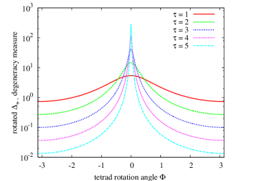
Figure 2: Profiles of the behavior of the degeneracy measure $\Delta_{ij}$ under tetrad rotations of the form in Eqs. (23) from a quasi-Kinnersley tetrad, for various values of a fiducial time coordinate, assuming that this degeneracy measure grows exponentially in this fiducial time coordinate for the true quasi-Kinnersley tetrad ($\Phi=0$). The peak value grows exponentially in time, by construction, but values well outside the peak decay exponentially in time. The peak sharpens as it grows, so that values slightly offset from the peak grow initially, and decay later.

the profile of $\Delta^{\prime}_{+-}:=|\lambda^{\prime}_{+}-\lambda^{\prime}_{-}|$, as a function of tetrad rotation angle $\Phi$ in Eq. (30), is shown for a few values of the fiducial time label $\tau$. Each curve is peaked, as in Fig. 1, at the quasi-Kinnersley tetrad. The value of this peak grows exponentially in $\tau$, while the values well outside the peak (representing more arbitrary tetrads) decay exponentially in $\tau$. What is of particular interest to us is the behavior near $\Phi=0$. Because the peak sharpens as it grows, values of $\Delta^{\prime}_{+-}$ slightly offset from $\Phi=0$ grow initially, and eventually decay. This behavior is more clearly visible in Fig. 3,

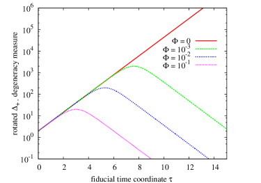
Figure 3: Behavior over time of the degeneracy measure $\Delta^{\prime}_{+-}(\Phi):=|\lambda^{\prime}_{+}-\lambda^{\prime}_{-}|$, for roots $\lambda^{\prime}_{\pm}$ given by Eq. (30), for a few values of the tetrad rotation parameter $\Phi$. Each curve initially grows exponentially in the time parameter $\tau$ before eventually falling. The more offset the tetrad is from the quasi-Kinnersley tetrad ($\Phi=0$), the sooner this turnaround occurs.

where $\Delta^{\prime}_{+-}$ is shown as a function of $\tau$ for various choices of the offset angle. For any fixed nonzero value of $\Phi$, the curve initially grows exponentially before eventually falling at the same rate. The smaller this rotation angle is, the later the curve turns around. So the nearer a tetrad is to quasi-Kinnersley, the longer it takes for $\Delta^{\prime}_{+-}$ to eventually decay as one might naively expect.

Incidentally, we should note that the “peak” in Fig. 2, and indeed in Fig. 1, is actually a saddle point if considered in a larger space of tetrad rotations. To keep the discussion simple, in Sec. II we considered only rotations in the local $\vec{e}_{1}$–$\vec{e}_{3}$ tangent plane. Had we considered the case of general rotations of the spatial tetrad, as in Eq. (1.2.34) of Ref. Penrose and Rindler (1987), we would have found that the degeneracy measure $\Delta_{ij}$ becomes infinite whenever the rotated tetrad $\vec{n}$ vector coincides with a principal null direction.

IV Interpreting degeneracy measures:

The geometrical underpinnings of the polynomial in Eq. (3), and the sense in which $\lambda$ constitutes a coordinate on the space of null rays, are most cleanly explained in the language of two-component spinors. Because many numerical relativists are unfamiliar with this formalism I will attempt to keep the discussion self-contained by briefly reviewing crucial elements as we go along. For a detailed account of spinor methods in spacetime geometry, see Refs. Penrose and Rindler (1987, 1988), or for a more compact treatment specifically geared to numerical relativists, see Ref. Stewart (1993).

Throughout this paper, objects with capital latin indices will be referred to as spinors, elements of a two-complex-dimensional vector space (or its higher tensorial orders). The complex conjugate of a spinor is also a spinor, but is defined in a different spinor space, because complex conjugation does not commute with multiplication by a complex scalar. To distinguish objects in spinor space from objects in the complex conjugate space, we will apply the standard convention of appending indices referring to the latter space with a prime:

$$\overline{\alpha^{A}}=\overline{\alpha}^{A^{\prime}}.$$ (31)

Spinors are useful in relativity theory because a simple correspondence exists between spinor space and Minkowski space (and therefore also to the tangent space to spacetime at any given point, given an orthonormal tetrad). From a spinor $\alpha^{A}$ a unique vector can be constructed in Minkowski space:

$$V^{a}=\alpha^{A}\overline{\alpha}^{A^{\prime}}{\sigma^{a}}_{AA^{\prime}},$$ (32)

where the ${\sigma^{a}}_{AA^{\prime}}$ are soldering forms, specifically referred to as Infeld–van den Waerden symbols, conventionally represented as Pauli matrices. In practice, the transformation provided by ${\sigma^{a}}_{AA^{\prime}}$ is often (and hereafter) taken as implied, with pairs of capital latin indices (one primed and one unprimed, with the same letter) taken to correspond abstractly to a single spacetime index.

Vectors defined directly from univalent spinors as in Eq. (32) turn out always to be null. For that reason univalent spinors can be understood as defining null vectors in spacetime. The standard geometrical interpretation of a univalent spinor (again, see Ref. Penrose and Rindler (1987); Stewart (1993)) is as a “null flag,” a null vector with a particular spacelike half-plane attached to it. This flag plane, encoded in the spinor’s complex phase, is unimportant for our current purposes.

The spacetime Weyl tensor can be written in terms of a four-index totally symmetric object called the Weyl spinor $\Psi_{ABCD}$ and the antisymmetric metric $\epsilon_{AB}$ on spinor space:

$$W_{abcd}=\Psi_{ABCD}\overline{\epsilon}_{A^{\prime}B^{\prime}}\overline{\epsilon}_{C^{\prime}D^{\prime}}.$$ (33)

Here, as in the introduction, $W_{abcd}$ refers to the Weyl tensor in its complex anti-self-dual form, $W_{abcd}:=C_{abcd}+i\hskip 2.84526pt{}^{\star}C_{abcd}$. A basic result in spinor algebra (due essentially to the fundamental theorem of algebra) is that any totally symmetric spin tensor can be decomposed into a symmetrized product of univalent spinors. In particular, for the Weyl spinor,

$$\Psi_{ABCD}=\alpha_{(A}\beta_{B}\gamma_{C}\delta_{D)},$$ (34)

for univalent spinors $\alpha_{A}$, $\beta_{B}$, $\gamma_{C}$, $\delta_{D}$ defined up to arbitrary complex scaling (any one of them can be scaled at the cost of inversely scaling another). These are referred to as principal spinors of $\Psi_{ABCD}$. Because the principal spinors are defined only up to a complex scaling, their corresponding null vectors are defined only up to an arbitrary real scaling, and their flag planes are completely undefined. The corresponding null vectors, defined up to scale, are the principal null directions of the Weyl tensor at the spacetime point under consideration.

Because the metric on spinor space, $\epsilon_{AB}$, is antisymmetric, all spinors have vanishing norm.

$$\alpha_{A}\alpha^{A}=0.$$ (35)

For this reason, the condition for $\alpha^{A}$ to be a principal spinor of the Weyl spinor is:

$$\Psi_{ABCD}\alpha^{A}\alpha^{B}\alpha^{C}\alpha^{D}=0.$$ (36)

To consider this equation more concretely, we introduce a basis, $\{o^{A},\iota^{A}\}$, in spinor space, normalized by the standard condition $\epsilon_{AB}o^{A}\iota^{B}=1$. Such a spin dyad is equivalent to a Newman-Penrose tetrad through the definitions $\ell^{a}=o^{A}\overline{o}^{A^{\prime}}$, $n^{a}=\iota^{A}\overline{\iota}^{A^{\prime}}$, $m^{a}=o^{A}\overline{\iota}^{A^{\prime}}$. Given a spin dyad, an arbitrary spin vector can be written as:

$$\alpha^{A}=\eta o^{A}+\xi\iota^{A},$$ (37)

for complex components $\eta$, $\xi$. Because we are only interested in spinors up to arbitrary complex scaling, we can divide by $\eta$ to let:

$$\alpha^{A}=o^{A}+\zeta\iota^{A},$$ (38)

where $\zeta=\xi/\eta$ is a possibly-infinite complex number, an element of the one-point-compactified complex plane, ${\mathbb{C}}\cup\{\infty\}$, the Riemann sphere.

Scaling an arbitrary spinor to be of this form, and inserting it into Eq. (36), the resulting equation is:

$$\Psi_{4}\zeta^{4}+4\Psi_{3}\zeta^{3}+6\Psi_{2}\zeta^{2}+4\Psi_{1}\zeta+\Psi_{0}=0,$$ (39)

where we have used the standard spinorial definition of the Weyl scalars:

$$\Psi_{0} := \Psi_{ABCD}o^{A}o^{B}o^{C}o^{D},$$ (40a)

$$\Psi_{1} := \Psi_{ABCD}o^{A}o^{B}o^{C}\iota^{D},$$ (40b)

$$\Psi_{2} := \Psi_{ABCD}o^{A}o^{B}\iota^{C}\iota^{D},$$ (40c)

$$\Psi_{3} := \Psi_{ABCD}o^{A}\iota^{B}\iota^{C}\iota^{D},$$ (40d)

$$\Psi_{4} := \Psi_{ABCD}\iota^{A}\iota^{B}\iota^{C}\iota^{D}.$$ (40e)

We thus find, comparing Eq. (3) with Eq. (39), that the quantity $\lambda$ can be interpreted as the complex stereographic coordinate $\zeta$ on the Riemann sphere, and in particular, as defining a spinor $\alpha^{A}$ of the form in Eq. (38) in a given spin dyad. Hereafter we will consider $\zeta$ and $\lambda$ to be the same quantity, and use the symbols interchangably.

This stereographic interpretation of $\zeta$ (or $\lambda$) is not merely a formality. As described in Chapter 1 of Ref. Penrose and Rindler (1987), the space of future-directed null rays at a point in spacetime is topologically a two-sphere. This can be demonstrated by cutting a future null cone with a spacelike 3-plane, given by $t=1$ in some local Minkowski coordinate system. Furthermore, if we choose a particular such cut, whose intersection with the null cone we will label $S^{+}$ and call the anti-celestial sphere, after Ref. Penrose and Rindler (1987), the metric induced on this two-sphere from that in the local Minkowski spacetime is:

$$ds^{2}=\frac{4d\zeta d\overline{\zeta}}{(1+\zeta\overline{\zeta})^{2}},$$ (41)

where for the coordinate we have chosen the $\zeta$ value of the spinor, of the form in Eq. (38), whose associated null direction intersects $S^{+}$. Applying the transformation to conventional spherical coordinates,

$$\zeta=e^{i\phi}\cot(\theta/2),$$ (42)

we arrive at the standard form of the unit sphere metric:

$$ds^{2}=d\theta^{2}+\sin^{2}(\theta)d\phi^{2}.$$ (43)

As a geometrical method for defining the nearness of two null directions to degeneracy, one can consider the metric (43) on the anti-celestial sphere. If $\zeta_{i}$ and $\zeta_{j}$ are two roots of Eq. (3), then one can translate them to spherical coordinates $(\theta_{i},\phi_{i})$, $(\theta_{j},\phi_{j})$ by inverting Eq. (42), and then use the metric distance function on the unit sphere, given by the haversine formula as:

$$\begin{split}\Theta_{ij}:=&2\arcsin\left\{\left(\sin^{2}\left[\left(\theta_{i}-\theta_{j}\right)/2\right]\right.\right.\\ &\left.\left.+\sin\theta_{i}\sin\theta_{j}\sin^{2}\left[(\phi_{i}-\phi_{j})/2\right]\right)^{1/2}\right\}.\end{split}$$ (44)

This can also be written directly in terms of the stereographic coordinates as:

$$\Theta_{ij}=2\arcsin\left[\frac{|\zeta_{i}-\zeta_{j}|}{\sqrt{(1+\zeta_{i}\overline{\zeta}_{i})(1+\zeta_{j}\overline{\zeta}_{j})}}\right].$$ (45)

As one can verify by a direct substitution of Eq. (24), this degeneracy measure is invariant under spatial rotations of the form in Eq. (23), or indeed any tetrad rotation that leaves the timelike tetrad leg invariant.

We must stress, however, that even this is not a totally invariant measure of degeneracy. In fact, there are fundamentally as many degrees of ambiguity in this measure as there are in $|\zeta_{i}-\zeta_{j}|$. The ambiguity in $\Theta_{ij}$ is encoded in the choice of cut one makes to the null cone in order to construct $S^{+}$. This can be interpreted physically as a result of the special relativistic effect known as “relativistic aberration of starlight,” by which the inferred geometry of the celestial (or as in this case, anti-celestial) sphere is conformally mapped under Lorentz boosts.

A geometrical interpretation of the degeneracy measure $\Delta_{ij}:=|\zeta_{i}-\zeta_{j}|$ can be found in spinor space. Two spinors $\alpha_{1}^{A}$ and $\alpha_{2}^{A}$ are proportional — and therefore their associated real null vectors are proportional — if and only if their antisymmetrized product vanishes:

$$\left[\alpha_{1},\alpha_{2}\right]:=\epsilon_{AB}\alpha_{1}^{A}\alpha_{2}^{B}=0.$$ (46)

It is tempting to use this quantity as a measure of the degeneracy of the null rays associated with $\alpha_{1}^{A}$ and $\alpha_{2}^{A}$, but we must remember to account for the scaling ambiguity of the spinors. If $\left[\alpha_{1},\alpha_{2}\right]$ is nonzero, then an arbitrary rescaling of either spinor, which should not alter any reasonable measure of the degeneracy of the null rays, would directly rescale $\left[\alpha_{1},\alpha_{2}\right]$. This ambiguity must be fixed by imposing a condition on the scaling of $\alpha_{1}^{A}$ and $\alpha_{2}^{A}$. One possibility, given a particular spin dyad $\left\{o^{A},\iota^{A}\right\}$, is to assume that the spinors are of the form (38), with $\alpha_{1}^{A}=o^{A}+\zeta_{1}\iota^{A}$, and $\alpha_{2}^{A}=o^{A}+\zeta_{2}\iota^{A}$. This condition can be stated for the associated null vectors $V_{1}^{a}$ and $V_{2}^{a}$ in terms of the Newman-Penrose tetrad as:

$$V_{i}^{a}n_{a}=-1,$$ (47)

for $i\in\{1,2\}$, along with the conditions that the $V_{i}^{a}$ are real null vectors, and where the Newman-Penrose tetrad vector $n^{a}$ is defined from the dyad spinor $\iota^{A}$ by $n^{a}:=\iota^{A}\overline{\iota}^{A^{\prime}}$. This subset of the future null cone can be visualized as its intersection with a null hyperplane defined by $t+z=\sqrt{2}$ in the local Minkowski coordinates. To the mind accustomed to Euclidean geometry, this intersection might be assumed to be a paraboloid. However, interestingly, the Lorentzian structure of the spacetime metric causes the intersection to be, in terms of the induced metric, a flat two-dimensional plane, with $\zeta$ a standard complex coordinate on this plane. In fact, the absolute value of the degeneracy measure $\left[\alpha_{1},\alpha_{2}\right]$, under this particular normalization condition, is precisely the quantity $\Delta_{12}=|\zeta_{1}-\zeta_{2}|$. For this reason, the degeneracy measure used in Campanelli et al. (2009) can be understood as a geometric distance between the two associated principal null directions along the cut made by a null hyperplane through the future null cone.

The degeneracy measure $\Theta_{ij}$ introduced in Eq. (45) can similarly be understood in terms of the symplectic product $\left[\alpha_{1},\alpha_{2}\right]$. If the condition on the null vectors associated with the $\alpha_{i}^{A}$ is taken to be that $\vec{V}_{i}\cdot\vec{e}_{0}=-1$, for a timelike tetrad vector defined from a Newman-Penrose tetrad through Eqs. (22), rather than $\vec{V}_{i}\cdot\vec{n}=-1$, then the spinors must be scaled as:

$$\alpha_{i}^{A}=\frac{1}{\sqrt{1+\zeta_{i}\overline{\zeta}_{i}}}\left(o^{A}+\zeta_{i}\iota^{A}\right).$$ (48)

In this case the absolute value of $\left[\alpha_{1},\alpha_{2}\right]$ becomes:

$$\left|\left[\alpha_{1},\alpha_{2}\right]\right|=\frac{|\zeta_{1}-\zeta_{2}|}{\sqrt{\left(1+\zeta_{1}\overline{\zeta}_{1}\right)\left(1+\zeta_{2}\overline{\zeta}_{2}\right)}},$$ (49)

essentially equivalent to $\Theta_{12}$, as defined in Eq. (45).

The distinction between the degeneracy measures $\Delta_{ij}$ and $\Theta_{ij}$ can therefore be understood as a distinction between two different realizations of the geometry of the space of null rays at a point. If the geometry in this space is inferred by cutting the null cone with a null hyperplane, the distance function on the set of null rays is given by $\Delta_{ij}$. If the cut is taken by a spacelike hyperplane, the distance is given by $\Theta_{ij}$.

The ambiguity of these distance functions stems from the ambiguity of these cuts. Fundamentally there are equally many degrees of ambiguity in both types of cut. A spacelike hyperplane can be boosted in any of three directions, translating into three continuous degrees of ambiguity for $\Theta_{ij}$ at each point in spacetime. A null hyperplane cut can also be given in terms of three degrees of freedom: the null normal to the hyperplane (for which there are two degrees of freedom, the anti-celestial sphere), and a parameter describing the translation of the hyperplane away from the vertex of the cone. This last degree of freedom also exists for spacelike hyperplanes, but because the intersection of the spacelike hyperplane with the null cone is compact (specifically a two-sphere), one can fix this translation degree of freedom by fixing the area of the sphere. In the case of a cut by a null hyperplane, the intersection is noncompact, so this degree of freedom cannot be fixed.

Though the degeneracy measure $\Theta_{ij}$ may be no more well-defined in general than $\Delta_{ij}$, there are still reasons to prefer it for purposes of defining a notion of approximate Petrov class. The main reason is that when a null hyperplane cut is made through a null cone, one special null ray is singled out: the one parallel to the hyperplane. Again, the intersection of the future null cone with a null hyperplane is itself a spacelike two-dimensional plane, and because the null ray parallel to the hyperplane never intersects the hyperplane, it is only represented on the intersection plane as a point at infinity. Eq. (47) shows that the null ray that gets mapped to the point at infinity is the one that points along the tetrad $\vec{n}$ vector. This is the behavior that we saw in Sec. III. The quasi-Kinnersley tetrad naturally adapts itself to the principal null directions in the ringdown to Kerr geometry, such that two of them fall toward the origin of the $\zeta$ plane and two approach infinity. This is because the quasi-Kinnersley tetrad is designed to adapt itself to nearly-degenerate principal null directions. To the extent that the numerical tetrad approximates a quasi-Kinnersley tetrad (a common implicit hope for the extraction of gravitational waveforms) this behavior will be seen also in numerical simulations. An example of this will be seen in the next section.

V Numerical Results

Our numerical implementation of these mathematical tools begins, as in Ref. Campanelli et al. (2009), with the fourth-order polynomial in Eq. (3). We begin by computing the Weyl scalars in a reference tetrad. The timelike orthonormal tetrad leg $\vec{e}_{0}$ is taken to be the normal to the spatial slice, and the spacelike orthonormal tetrad legs are constructed from a Gram-Schmidt orthogonalization of the basis vectors of a spherical-like coordinate system within the spatial slice, essentially similar to the method in Campanelli et al. (2009). This tetrad is singular at the $z$ axis, as the complex phase of the $\vec{m}$ leg becomes undefined due to the coordinate singularity of the spherical chart, but all quantities we present will be independent of this complex phase, and thus will have well-defined values on the axis.

Our code computes the electric and magnetic parts of the Weyl curvature tensor directly from data on the spatial slice, using Gauss-Codazzi relations and assuming the Einstein equations are satisfied and that no matter fields are present:

$$E_{ij} = \left({}^{3}R_{ij}+KK_{ij}-K_{ik}K_{j}^{k}\right)_{\rm STF}$$ (50)

$$B_{ij} = \left(\epsilon_{i}{}^{mn}D_{m}K_{nj}\right)_{\rm STF}.$$ (51)

Here, $K_{ij}$ is the extrinsic curvature of the spatial slice, $D_{i}$ is the torsion free covariant derivative compatible with the spatial metric, ${}^{3}R_{ij}$ its Ricci curvature, $\epsilon_{ijk}$ the spatial Levi-Civita tensor, and the subscript ${\rm STF}$ means that the quantity in brackets is made symmetric and tracefree in the indices $i$ and $j$. Once these tensors are computed, we construct the Weyl scalars from them as in Eqs. (4) of Ref. Nerozzi (2007), using the radial tetrad leg for $\vec{u}$, and the polar leg plus $i$ times the azimuthal leg for $\vec{m}$.

Once the Weyl scalars are known, one can go about solving for the roots $\lambda_{i}$ of Eq. (3). We do so point by point on the computational grid with simple Newton-Raphson iteration and polynomial deflation Press et al. (2007). In many cases, these methods are conventionally followed by root polishing — using the computed roots of the deflated polynomials as initial guesses in new Newton-Raphson iterations of the initial polynomial, with the hope of correcting roundoff error accumulated in the deflation process — but in this case root polishing has no noticeable effect. This is presumably because the roots under consideration are very nearly degenerate, so error in the Newton-Raphson iterations themselves dominates the error accumulated in the polynomial deflation.

As in Ref. Campanelli et al. (2009), we focus our attention on a simulation of the ringdown of a binary black hole merger to Kerr geometry. The simplest example of such a merger is one following the inspiral of two equal mass nonspinning black holes in a noneccentric configuration. This data set was presented in detail in Ref. Scheel et al. (2009), and the multipolar structure of the post-merger horizon was studied in Ref. Owen (2009). In the former paper, it was noted that two independent measures of black hole spin, designed to agree if the final black hole is Kerr, agreed to well within the estimated accuracy of the numerical truncation. In the latter paper, this correspondence was studied in much greater detail, demonstrating that all of the multipole moments on the apparent horizon that we were able to compute agreed very well with those of the Kerr horizon (see Refs. Schnetter et al. (2006); Jasiulek (2009) for a similar analyses). While these provide a very compelling case that the final black hole is Kerr, they do not present a major benefit of the methods described here and in Ref. Campanelli et al. (2009): being fully local. The degeneracy measures described here can be computed independently at each point in spacetime, rather than simply for the apparent horizon as a whole. In this way one can imagine demonstrating not just the fact that a spacetime is settling down to Kerr geometry, but where it is doing so more quickly and more slowly, and possibly even the relationship between the approach to Kerr geometry and the presence of gravitational radiation.

This locality of the approximate Petrov classification system, while beneficial for the reasons described above, unfortunately comes at the cost of another type of gauge ambiguity. If one wishes to investigate the time dependence of the degeneracy measures, then one must choose a worldline in spacetime along which to compute these quantities. In principle one could reduce this ambiguity, for example by computing along timelike geodesics, or worldlines preferred by some sort of symmetry, if any exist. For example, the symmetries inherent in a merger of equal mass, initially nonspinning holes provide at least one preferred axis for consideration. The initial data satisfy a discrete symmetry under 180-degree rotations about a certain axis, taken in our simulations to be the coordinate $z$ axis, along which the initial “orbital angular momentum vector” can be intuitively said to point. To the extent that the numerical simulation preserves this discrete symmetry, the $z$ axis sweeps out a geometrically well-defined worldsheet in spacetime. In principle this timelike worldsheet could be restricted to a single well-defined timelike worldline, on which data can be extracted, by intersecting the worldsheet with a level surface of some curvature invariant. Here, however, we do not go to such lengths, electing instead to follow coordinate worldlines, as in Ref. Campanelli et al. (2009), but paying special attention to the symmetry axis.

In Fig. 4,

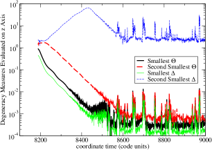
Figure 4: The ringdown after the merger of two equal mass, initially nonspinning holes. The curves show the behavior of the two smallest values of each of the degeneracy measures $\Delta_{ij}$ and $\Theta_{ij}$, with respect to coordinate time, evaluated at $z=4.5$, $x=y=0$ in an asymptotically inertial coordinate system. The heavier curves show the two values of the $\Theta_{ij}$ measure, the lighter curves the $\Delta_{ij}$ measure. The solid curves show the smaller values of these measures, and the dashed curves the larger. The symmetries along this axis force the tetrad to satisfy the basic conditions of a “quasi-Kinnersley” tetrad, as described in section III, and the results of that section explain the initial exponential growth of the higher $\Delta_{ij}$ curve.

data are shown for the two smallest — smallest among the various possible root pairings — values of the degeneracy measures $\Delta_{ij}$ and $\Theta_{ij}$ evaluated at the coordinate location $x=y=0$, $z=4.5$ as a function of coordinate time after the formation of the common apparent horizon in the dataset described in Ref. Scheel et al. (2009). Because the tetrad is, by construction, adapted to the symmetry axis at this location, it is forced to be “transverse” in the sense of Sec. III (a fact which we have verified by a direct inspection of the computed values of $|\Psi_{1}|$ and $|\Psi_{3}|$). In Fig. 4, we initially see exponential growth in the second-smallest root difference $\Delta_{ij}$, as one would expect from the considerations of Sec. III. Eventually, this exponential growth gives way to exponential decay, similar to the behavior seen in Fig. 3. This occurs because the data we compute here are actually interpolated to the polar axis from data on grid points slightly offset from it. On these grid points, the tetrad differs slightly from the quasi-Kinnersley tetrad, as in the discussion near the end of Sec. III. One might hope that this eventual decay would only occur on these offset grid points, and that the data interpolated to the axis would grow indefinitely as $\sqrt{-6\Psi_{2}/\Psi_{4}}$, but as the black hole settles down the growing peak in Fig. 2 shrinks in width, so eventually one would expect it not to be resolved by the spectral discretization. Incidentally, we have confirmed that the rates of exponential decay in the decaying curves, and the rate of exponential growth in the growing curve, each roughly equal half of the damping rate of the least-damped quasinormal mode of a Kerr black hole of the same final mass and spin as our final remnant. One would expect this from Eq. (29). The most important issue to note about Fig. 4, though, is the discrepancy between the picture implied by the $\Delta_{ij}$ values, and that implied by the $\Theta_{ij}$ values. The highest and lowest curves are the two relevant values of $\Delta_{ij}$. At early times, even the qualitative behavior of these curves are different, one growing and one decaying. Even at late times, when both curves decay exponentially (and eventually settle to fixed limits due to numerical truncation error), they still differ by four orders of magnitude. If $\Delta_{ij}$ were naively interpreted as defining the “nearness” to any Petrov class, then the response to Fig. 4 would be that the final result of the numerical simulation is of Petrov Type II, not Type D, on this axis. The other two curves in Fig. 4 tell a very different story. The two heavier curves in Fig. 4 show the two smallest values of the $\Theta_{ij}$ measure. Both curves fall exponentially at the same rate, and they lie within roughly a factor of ten of one another throughout the entire ringdown. According to $\Theta_{ij}$ the spacetime falls quite unambiguously to Petrov Type D on the polar axis.

The behavior at different coordinate locations is less striking, but shows roughly similar features. Fig. 5

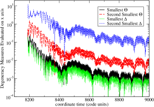
Figure 5: The two smallest values of the degeneracy measures $\Delta_{ij}$ and $\Theta_{ij}$ evaluated at the coordinate location $x=4.5$, $y=z=0$ in the ringdown after a merger of equal-mass, initially nonspinning black holes, as in Fig. 4. The lighter curves, which are generally the highest and lowest curves, are the two values of the $\Delta_{ij}$ measure. The heavier curves represent the $\Theta_{ij}$ measure. Initial growth of the larger $\Delta_{ij}$ value is still present, but less striking than in Fig. 4. Nonetheless, the two $\Delta_{ij}$ values again differ by multiple orders of magnitude, while the two $\Theta_{ij}$ values generally differ by only one.

presents the same quantities as Fig. 4 computed instead at $x=4.5$, $y=z=0$. Again, the highest and lowest curves are the two relevant values of $\Delta_{ij}$. The higher one grows slightly (on average) in the early ringdown, but settles into exponential decay quite a bit sooner than in Fig. 4, and throughout the ringdown remains separated from the values in the lowest curve by roughly two to three orders of magnitude. This still, however, provides a marked contrast from the two $\Theta_{ij}$ curves, which again lie within roughly a single order of magnitude of one another throughout the ringdown. A particularly interesting feature is visible in the uppermost curve of Fig. 5 from the beginning of the post-merger dataset to roughly the coordinate time $8275$. This time frame is magnified in Fig. 6.

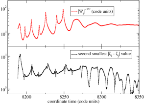
Figure 6: Magnification of the highest curve in Fig. 4. The sharp peaks in the bottom curve before time $8275$ imply that principal null directions are occasionally crossing the tetrad legs. The upper curve corroborates this by explicitly showing that the absolute value of the Weyl scalar $\Psi_{4}$ approaches zero at times coincident with these sharp peaks.

Because the spacetime is symmetric under reflections across the $z=0$ plane, the spatial projections of the principal null directions on this plane must either be tangent to the plane, or otherwise reflection-symmetric across it. The jagged peaks in Fig. 6 imply that the former possibility seems to apply here. When the tetrad $\vec{n}$ vector happens to point along a principal null direction, the corresponding $\zeta$ value of the polynomial root becomes infinite. If the spatial projections of two of the principal null directions lie in the same plane as the spatial projection of the tetrad $\vec{n}$ vector, and they oscillate in direction, repeatedly crossing the spatial projection of $\vec{n}$ (due either to physical or gauge effects), then one would expect the $\Delta_{ij}$ values involving these principal null directions to show sharp, repeating peaks, such as those in Fig. 6. Eventually, such crossings could be expected to stop as the angle between the spatial projections of the principal null directions becomes small and as gauge and physical oscillations become less wild. After roughly $t=8275$ in these code units the oscillations in this curve become more smooth, implying that the principal null directions are no longer crossing $\vec{n}$.

Figure 7

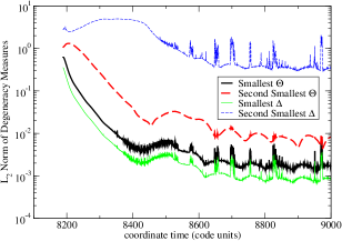
Figure 7: $\L_{2}$ norms of the two smallest values of $\Delta_{ij}$ and $\Theta_{ij}$, integrated over a thick spherical shell extending from just within the apparent horizon, $r=2.2$ in code coordinates, to an outer boundary at $r=5$ code coordinates. Again, both values of $\Theta_{ij}$ fall quickly to zero at the same rate, while the larger $\Delta_{ij}$ value hangs up initially, and eventually falls only to a level over two orders of magnitude above its smaller counterpart.

presents $L_{2}$ norms of the same degeneracy measures for the same ringdown dataset. While this avoids the choice of a specific coordinate location for observation, we should note that there is still a certain amount of coordinate ambiguity in this quantity. The $L_{2}$ norm is only over a certain subset of the spatial slice. The inner boundary is the excision boundary of the simulation, slightly inside the apparent horizon. The outer boundary is a boundary of subdomains in the simulation, with coordinate radius 5. The purpose of this outer boundary is to avoid numerical difficulties when the Weyl scalars become too small to calculate accurately the roots of the polynomial in Eq. (3). Again in Fig. 7, we see the larger value of $\Delta_{ij}$ hanging up while both values of $\Theta_{ij}$ decay exponentially.

VI Discussion

The primary goal of this paper has been to explain the peculiar behavior, noted in Ref. Campanelli et al. (2009), that the spacetimes of binary black hole mergers seem to “hang up” in Petrov Type II, and if they fall to Type D at all (according to one’s choice of tolerance), they do so much later.

Properly clarifying this issue has required us to investigate the geometrical meaning of the polynomial in Eq. (3) and the measure of degeneracy principally used in Ref. Campanelli et al. (2009), the absolute value of the difference of any two roots, $\Delta_{ij}:=|\lambda_{i}-\lambda_{j}|$. The true space of interest is the space of future-directed null rays at a point, the so-called anti-celestial sphere. As argued in Sec. IV, the complex quantity $\lambda$ acts as a coordinate on this two-dimensional space. It should therefore not be surprising that $\Delta_{ij}$, a coordinate distance, fails to represent geometries in the space of null rays, since it is impossible to cover a topological sphere with a single coordinate chart without the presence of coordinate singularities.

It would therefore seem that the right thing to do would be to consider truly geometrical distances in the space of null rays as defining the nearness of principal null directions to one another. This approach, unfortunately, is clouded by the nonexistence of a preferred metric structure on the anti-celestial sphere. The anti-celestial sphere has a six-dimensional conformal group, corresponding to the proper Lorentz group of Minkowski spacetime. While this group carries a three-dimensional subgroup of isometries — corresponding to rotations — which have no effect on the “distances” between any two null rays, the three remaining dimensions — corresponding to boosts — conformally rescale the metric on the space of null rays. For this reason, fixing a unique geometry on the space of null rays requires fixing a unique “observer” with respect to which this boost freedom is fixed. In the introduction, we described similar difficulties in attempting to define a concept of approximate Petrov class by algebraic means.

In Sec. IV we also presented a geometrical interpretation of the quantity $\Delta_{ij}$. Rather than simply as a coordinate distance on the space of null rays, $\Delta_{ij}$ can be interpreted as a metric distance along the cut of a null cone made by a null hyperplane. In a sense, one is here adapting the metric on the space of null rays to a null observer. Similarly, $\Theta_{ij}$ is a distance function on the intersection of the future null cone with a spacelike plane orthogonal to our timelike observer.

There are equally many degrees of freedom in cutting the null cone with a spacelike hyperplane as there are in cutting it with a null hyperplane (once one restricts the spacelike cuts to normalize the area of the anti-celestial sphere, a restriction that cannot be made on null hyperplanes because the intersection is noncompact). For this reason the degeneracy measure that we have introduced, $\Theta_{ij}$ in Eq. (45), cannot be considered fundamentally any more invariant than $\Delta_{ij}$, though in practice it is easier to imagine a fleet of preferred timelike observers than of null observers, such as stationary observers in stationary spacetimes, observers adapted to timelike approximate Killing vectors in approximately stationary spacetimes (if such vectors can be reasonably defined), or freely falling observers following timelike geodesics from infinity. We have not, however, attempted to find any such preferred classes of observers in the numerical results presented here, either for fixing the geometry on the space of null rays or for fixing the worldlines along which data are extracted. The main value of the new degeneracy measure $\Theta_{ij}$ is not that it is more gauge-invariant, but rather that it naturally captures the compactness of the space of null rays, and thereby avoids relegating any particular null ray to a point at infinity.

The need to avoid relegating any null ray to a point at infinity is particularly acute in practice, as the rays at infinity in the physically preferable quasi-Kinnersley tetrads become the principal null directions themselves as a spacetime settles down to Kerr geometry. This behavior was investigated in Sec. III. As principal null directions relax to degeneracy at the point at infinity in $\lambda$ space, the degeneracy measure $\Delta_{ij}$ grows exponentially rather than decaying exponentially as one would naively expect. While the tetrads used in numerical simulations are not commonly quasi-Kinnersley tetrads, there is generally an implicit hope, for purposes of wave extraction, that they are close to it in some rough sense. Indeed, as is visible in Fig. 4, this nonintuitive behavior in the quasi-Kinnersley tetrad can corrupt measurements of $\Delta_{ij}$ in even a simple coordinate-adapted tetrad (cf. Fig. 3).

The other figures in Sec. V tell much the same story, though in somewhat less dramatic terms. Fig. 6 shows indications of principal null directions directly crossing the tetrad null vectors, repeatedly causing the null directions to be represented by the point at infinity in $\lambda$ space, due purely to the choice of spatial tetrad. Fig. 7 shows that the hangups in the degeneracy measure $\Delta_{ij}$ are not limited to the partially symmetry-preferred $x$ and $z$ axes. In fact, $\Delta_{ij}$, computed everywhere in a tetrad adapted to spherical coordinates, clearly shows this hangup in Petrov Type II even in an integral $L_{2}$ norm, while $\Theta_{ij}$ does not.

Another motivation of this paper has been to provide further evidence that the final remnants of our black hole merger simulations are Kerr black holes. This was indeed the central focus of Ref. Campanelli et al. (2009), and they even went so far as to demonstrate that their final black hole has no NUT charge or acceleration (as in the C-metrics; see Ref. Griffiths and Podolský (2009)), an issue that we have not explored here.

The question of whether a black hole is “settling down to Kerr” can be attacked at a variety of levels. In a recent paper Owen (2009), we studied the question at a quasilocal level, verifying that the quasilocal source multipole moments of the black hole settle to the values required by the Kerr geometry (see also Refs. Schnetter et al. (2006); Jasiulek (2009)). More recently, Ref. Bäckdahl and Kroon (2010) presented theoretical tools for approaching the question at a global level (global on any given spacelike slice). The approach taken in Ref. Campanelli et al. (2009) was in part local (measurement of $\Delta_{ij}$), and in part global. The method by which Campanelli et al. verified the vanishing of the NUT charge and acceleration involved limits of curvature invariants to large radii. If one wishes to rule out NUT charge or acceleration at a local level, to provide a more cohesive picture when combined with local algebraic degeneracy measures, this can be done with quantities presented in Ref. Ferrando and Sáez (2009), though as described in the introduction of this paper, collapsing tensorial quantities to scalar quantities would require a positive-definite background metric, which could require fixing a slicing or a threading of spacetime.