A GIBBS DISTRIBUTION THAT LEARNS FROM GA DYNAMICS

1 Introduction

Genetic Algorithm (GA) is a heuristics to find the best possible solution for combinatorial optimization problems and it is based on several relevant operators such as selection, crossover and mutation on the gene configurations (strings) leading to transition from one state to the others. This probabilistic algorithm was firstly introduced in the book Adaptation in Natural and Artificial Systems by John Holland in 1975 [H.Holland, 1975] and now it has been widely used in various research fields and established as one of the effective algorithms to find the solution within reasonable computational time [E.Goldberg, 1989].

However, it does not mean that the GA can be automatically applied to any problem and can find the candidates of the solutions immediately. We should choose the suitable information representation of each gene (member) in population (ensemble) for a given problem and the parameters which control the operations should be set to the optimal values. Basically, these operations except for the selection, which is dependent on the fitness, are defined as procedures to generate the states randomly and the operations do not always confirm to increase the fitness value. To make matter worse, there are few mathematical justification for the GA to make the system to convergence to one of the best possible solution.

From this fact in mind, in this paper, in order to figure out the statistical properties of GA from the view point of thermodynamics, we introduce a learning algorithm of Gibbs distributions from training sets which are gene configurations generated by GA. A procedure of average-case performance evaluation for genetic algorithms is examined. The learning algorithm is constructed by means of minimization of the Kullback-Leibler information between a parametric Gibbs distribution and the empirical distribution of gene configurations. The formulation is applied to the solvable probabilistic models having multi-valley energy landscapes, namely, the spin glass chain [Li, 1981, H.Chen and K.Ma, 1982] and the Sherrington-Kirkpatrick model [Sherrington and Kirkpatrick, 1975] in statistical physics. By using computer simulations, we discuss the asymptotic behaviour of the effective temperature scheduling and the residual energy induced by the GA dynamics. We also reveal the operator-dependence of the behaviour.

As well-known, a study focusing on the distribution of gene configurations in GA itself is not a bran-new approach. Actually, the so-called Estimation of Distribution Algorithm (EDA) [Baluja, 1994, Pelikan et al., 1999, Pelikan et al., 2000, Pelikan et al., 2002, L.Shapiro, 2005, L.Shapiro, 2006, S.Correa and L.Shapiro, 2006] is a well-known and established approach to find the best possible solution by estimating the distribution of gene configuration during the GA dynamics and one can use the distribution to produce the genes in the next generation. In fact, a lots of such studies have been done for various problems.

For instance, Prugel-Bennett and Shapiro [Prugel-Bennett and L.Shapiro, 1994, Prugel-Bennett and L.Shapiro, 1997] evaluated the time evolution of the cummulants of distributions and discussed the statistical properties of GA from the dynamical point of view. Suzuki [Suzuki, 1995, Suzuki, 1998, Suzuki, 2005] represented the relationship between the gene configurations by graphical models and estimated the joint probability or the marginal probability of the genes by making use of Belief propagation on the graphical models.

Nevertheless there exist such extensive studies, in the present study, we choose a Gibbs distribution which is specified by a single parameter, namely, temperature $T$ and learns the distribution (the effective temperature) from the gene configurations produced by GA. Thus, we attempt to figure out the average-case performance of GA from the view point of temperature scheduling in simulated annealing. Moreover, the evaluation of average-case performance is partially carried out analytically by choosing the energy function of solvable spin glass models. These points are remarkable distinctions of our approach in the present paper.

This paper is organized as follows. In the next section, we mention the relationship between the GA and simulated annealing from the view point of the distribution of ensembles (population) on Markovian process. In section 3, we explain our formulation and tools to investigate the average-case performance of the GA. We construct the Boltzmann-machine-type learning equation via the minimization of Kullback-Leibler information between the empirical distribution of GA and a Gibbs distribution with respect to the effective temperature. The validity of a Gibbs form of the distribution is confirmed by the so-called Holland’s condition. The learning equation is rewritten in terms of optimization of the energy function for Ising spin systems. The concept of average-case performance is mentioned, namely, the so-called self-averaging properties for physical quantities and the replica method to carry out the average are introduced. In the next section 4, we introduce our benchmark test problem, namely, the combinatorial optimization problem having the energy function of the so-called spin glasses. The mathematically tractable spin glasses, namely, spin glass chain and the Sherrington-Kirkpatrick model are introduced and their statistical properties are revealed. In section 5, we explain the set-up of our numerical experiments and the results are reported in the next section 6. The last section is devoted to concluding remarks.

2 GA and SA

As we mentioned, in this paper, we consider the statistical properties of GA from the view point of thermodynamics. In simple GA, we define each gene configuration (member) by a string of binary variables with length $N$, that is, $\bm{s}=(s_{1},s_{2},\cdots,s_{N}),s_{i}\in\{-1,+1\}$, and we attempt to make each configuration in ensemble with size $M$ to the state which gives a minimum of the energy function $H(\bm{s})$, say, $\bm{s}_{*}$ D The problem is systematically solved by GA if the system evolves according to a Markovian process and the gene distribution $P_{GA}^{(t)}(\bm{s})$ at time (generation) $t$ might converge as $P_{GA}^{(t)}(\bm{s})\to P_{GA}^{(\infty)}(\bm{s})$ and we have

$$P_{GA}^{(\infty)}(\bm{s})=\delta(\bm{s}-\bm{s}_{*})=\prod_{i=1}^{N}\delta(s_{i}-s_{i*}).$$ (1)

On the other hand, one of the effective heuristics which is well-known as Simulated Annealing (SA) [Kirkpatrick et al., 1983, Geman and Geman, 1984] is achieved by inhomogeneous Markovian process. The process is realized by Markov chain Monte Carlo method (MCMC) which leads to an equilibrium Gibbs distribution at temperature $T=\beta^{-1}$ (from now on, the $\beta$ is referred to as ‘inverse temperature’), namely,

$$P_{B}^{(t)}(\bm{s})=\frac{{\rm e}^{-\beta^{(t)}H(\bm{s})}}{Z},\,\,\,\,Z=\sum_{\bm{s}}{\rm e}^{-\beta^{(t)}H(\bm{s})}.$$ (2)

In SA, the temperature is scheduled very slowly in time as $\beta^{(\infty)}\to\infty$ ($T^{(\infty)}\to 0$), and then, we can solve the problem as

$$P_{B}^{(\infty)}(\bm{s})=\delta(\bm{s}-\bm{s}_{*})=\prod_{i=1}^{N}\delta(s_{i}-s_{i*}).$$ (3)

Therefore, both the GA and the SA share a concept to make the distribution convergence to a single (or several) delta-peak(s) at the solution(s). However, in general, the Markovian (dynamical) process of GA is very hard to treat mathematically due to the global transition between the states by the crossover or, especially, the mutation operator, whereas the SA causes only local transitions between the states. From the view point of EDA, the dynamics of GA should lead to an empirical distribution of states. As we shall mention later on, the distribution is more likely to be a Gibbs one and it might be reasonable approach to grasp the shape through the Gibbs form (effective temperature) of the distribution.

3 Formulation and tools

In this section, we explain our formulation and several tools to evaluate the average-case performance of GA through the effective temperature scheduling of the Gibbs distribution that is trained from gene configurations of simple GA.

3.1 Kullback-Leibler information

We start our argument from the distance between an empirical distribution from GA dynamics $P_{GA}^{(t)}(\bm{s})$ and a Gibbs distribution $P_{B}^{(t)}(\bm{s})$ at the effective temperature $T=\beta^{-1}$. The distance is measured by the following Kullback-Leibler information (KL)

$$KL(P_{GA}\|P_{B})=\sum_{\bm{s}}P_{GA}(\bm{s})\log\left\{\frac{P_{B}(\bm{s})}{P_{SA}(\bm{s})}\right\}$$ (4)

where the summation with respect to all possible gene configurations $\bm{s}=(s_{1},\cdots,s_{N})$ is defined by

$$\sum_{\bm{s}}(\cdots)\equiv\sum_{s_{1}=\pm 1}\cdots\sum_{s_{N}=\pm 1}(\cdots).$$ (5)

In this paper, we represent each component of gene configurations by $s_{i}=\pm 1$ instead of $s_{i}=0,1$ because we choose the cost function of spin glasses to be minimized as a benchmark test later on. The ‘spin’ here means a tiny magnet in atomic scale-length and $s_{i}=+1$ stands for ‘up-spin’ and vice versa. We should keep in mind that the above distance is dependent on the inverse temperature $\beta$. Thus, we obtain the following Boltzmann-machine-type learning equation with respect to $\beta$ as

$$\frac{d\beta}{dt} = -\frac{\partial KL(P_{GA}^{(t)}\|P_{B}^{(t)})}{\partial\beta}=\sum_{\bm{s}}P_{GA}^{(t)}(\bm{s})\cdot\frac{{\partial P_{B}^{(t)}(\bm{s})}/{\partial\beta}}{P_{B}^{(t)}(\bm{s})}.$$

We naturally expect that the effective temperature evolves so as to minimize the KL information for each time step. When both distributions become identical one in the limit of $t\to\infty$, namely, $P_{GA}^{(\infty)}(\bm{s})=P_{B}^{(\infty)}(\bm{s})$, we obtain

$$\frac{d\beta}{dt} = \sum_{\bm{s}}P_{GA}^{(\infty)}(\bm{s})\cdot{\{{\partial P_{B}^{(\infty)}(\bm{s})}/{\partial\beta}}\}/{P_{B}^{(\infty)}(\bm{s})}$$ (7)

$$= ({\partial}/{\partial\beta})\sum_{\bm{s}}P_{B}^{(\infty)}(\bm{s})$$

$$= ({\partial}/{\partial\beta})\sum_{\bm{s}}\delta(\bm{s}-\bm{s}_{*})={\partial\alpha}/{\partial\beta}=0$$

and the time evolution of inverse-temperature then stops. We should notice that $\alpha\equiv\sum_{\bm{s}}\delta(\bm{s}-\bm{s}_{*})$ is the number of degeneracy at the lowest energy states.

3.1.1 The Holland’s condition

Before we examine the time-dependence of the effective temperature $\beta$, we comment on the validity of the choice of a Gibbs form as the distribution. John Holland mentioned that the algorithm might be effective if the probability $P(\mathcal{H},t)=\sum_{i\in\mathcal{H}}p_{i}(t)$ that a schema $\mathcal{H}$ appears at generation (time step) $t$ follows the following condition as a kind of ‘Master equation’ of probabilistic flow:

$$\frac{dP(\mathcal{H},t)}{dt}=f(\mathcal{H},t)-P(\mathcal{H},t)f(\mathcal{J},t)$$ (8)

where $\mathcal{J}$ stands for an arbitrary schema which is different from the $\mathcal{H}$ and $p_{i}(t)$ is a probability that a gene configuration $i$ appears at generation $t$ [H.Holland, 1975]. $f(\mathcal{H},t)$ denotes the average fitness of the schema $\mathcal{H}$ at generation $t$:

$$f(\mathcal{H},t)=\sum_{i\in\mathcal{H}}g(i)p_{i}(t).$$ (9)

The above equation means that the probability that a $\mathcal{H}$ appears increases proportional to the average fitness value of $\mathcal{H}$ and it also decreases proportional to the average fitness values $f(\mathcal{J},t)\equiv\sum_{i\in\mathcal{J}\neq\mathcal{H}}g(i)p_{i}(t)$.

One can easily show that the above condition is satisfied by a Gibbs distribution having the form:

$$p_{i}(t)=\frac{{\exp}[\beta_{t}g(i)]}{\sum_{j\in\mathcal{J}}{\exp}[\beta_{t}g(j)]}.$$ (10)

For simplicity, we assume that the inverse temperature increases linearly in time as $\beta_{t}=t$. Then, the above (10) leads to

$$p_{i}(t)=\frac{{\exp}[tg(i)]}{\sum_{j\in\mathcal{J}}{\exp}[tg(j)]}.$$ (11)

Taking the derivative of both sides of the above equation with respect to $t$, we have

$$\frac{dp_{i}(t)}{dt} = \frac{g(i)\,{\rm e}^{tg(i)}(\sum_{j\in\mathcal{J}}{\rm e}^{tg(j)})-{\rm e}^{tg(i)}\sum_{j\in\mathcal{J}}g(j){\rm e}^{tg(j)}}{(\sum_{j\in\mathcal{J}}{\rm e}^{tg(j)})^{2}}$$ (12)

$$= \frac{g(i){\rm e}^{tg(i)}}{\sum_{j\in\mathcal{J}}{\rm e}^{tg(j)}}-\left(\frac{{\rm e}^{tg(i)}}{\sum_{j\in\mathcal{J}}{\rm e}^{tg(j)}}\right)$$

$$\times \left(\frac{\sum_{j\in\mathcal{J}}g(j){\rm e}^{tg(i)}}{\sum_{j\in\mathcal{J}}{\rm e}^{tg(j)}}\right)$$

$$= p_{i}(t)g(i)-p_{i}(t)\sum_{j\in\mathcal{J}}g(j)p_{j}(t).$$

Taking the derivative of $P(\mathcal{H},t)=\sum_{i\in\mathcal{H}}p_{i}(t)$ with respect to $t$ and substituting the above (12) into the right hand side of the equation, we obtain

$$\frac{dP(\mathcal{H},t)}{dt} = \sum_{i\in\mathcal{H}}\frac{dp_{i}(t)}{dt}$$ (13)

$$= \sum_{i\in\mathcal{H}}\left\{p_{i}(t)g(i)-p_{i}(t)\sum_{j\in\mathcal{J}}g(j)p_{j}(t)\right\}$$

$$= \sum_{i\in\mathcal{H}}p_{i}(t)g(i)-\sum_{i\in\mathcal{H}}p_{i}(t)\sum_{j\in\mathcal{J}}g(j)p_{j}(t)$$

$$= f(\mathcal{H},t)-P(\mathcal{H},t)f(\mathcal{J},t)$$

where we used the definition (9) of average fitness of the schema $\mathcal{H}$ at generation $t$. This equation is nothing but the Holland’s condition (8). This result means that the empirical distribution of genes which are generated by GA dynamics is more likely to be a Gibbs distribution or can be well-approximated by a Gibbs distribution specified by the inverse temperature $\beta$ if the GA effectively finds the solution for a given optimization problem. This fact provides us a justification of the present approach to make a Gibbs distribution learns from the GA dynamics.

3.2 Learning equation for spin systems

In the previous section, we formulated the learning equation for general problems and discussed some key properties including the Holland’s condition in the formulation. Here we attempt to restrict ourselves to more particular problems, namely, we deal with a class of combinatorial optimization problems whose cost functions are described by the energy function of Ising model.

We first reformulate the equation (LABEL:eq:LE) by means of Ising spin systems having the energy function $H(\bm{s})=-\sum_{ij}J_{ij}s_{i}s_{j}$. For the case of positive constant spin-spin interaction $J_{ij}=J>0,\,\,\,\forall_{i,j}$, the lowest energy state is apparently given by $s_{i}=+1,\,\,\,\forall_{i}$ (all-up spins) or $s_{i}=-1,\,\,\,\forall_{i}$ (all-down spins). However, as we shall see in the following sections, for the case of randomly distributed $J_{ij}$ (the $\pm$ sign is also random), the lowest energy state is highly degenerated and it becomes very hard to find the state. It should be noted that the traveling salesman problem (TSP) (see e.g. [Mezard and Parisi, 1986]) or the $k$-satisfiability problem ($k$-SAT) (see e.g. [Monasson et al., 1999]) is rewritten in terms of optimization problems described by the variant of the above energy function of spin glasses.

Substituting the corresponding Gibbs distribution $P_{B}(\bm{s})={\exp}[-\beta H(\bm{s})]/\sum_{\bm{s}}{\exp}[-\beta H(\bm{s})]$ into equation (LABEL:eq:LE), the learning equation leads to

$$\frac{d\beta}{dt}=\sum_{\bm{s}}P_{GA}(\bm{s})\left(\sum_{ij}J_{ij}s_{i}s_{j}\right)$$ (14)

$$- \frac{\sum_{\bm{s}}(\sum_{ij}J_{ij}s_{i}s_{j})\,{\exp}[\beta\sum_{ij}J_{ij}s_{i}s_{j}]}{\sum_{\bm{s}}{\exp}[\beta\sum_{ij}J_{ij}s_{i}s_{j}]}$$

where the second term appearing in the right hand side of the above equation is internal energy of the system described by the Hamiltonian $H(\bm{s})=-\sum_{ij}J_{ij}s_{i}s_{j}$ at temperature $T=\beta^{-1}$, whereas the first term is the energy $H(\bm{s})$ averaged over the empirical distribution $P_{GA}(\bm{s})$ of GA. Then, we immediately find that the condition

$$\sum_{\bm{s}}P_{GA}(\bm{s})(\sum_{ij}J_{ij}s_{i}s_{j})=\sum_{\bm{s}}P_{B}(\bm{s})(\sum_{ij}J_{ij}s_{i}s_{j})$$ (15)

$$= \frac{\sum_{\bm{s}}(\sum_{ij}J_{ij}s_{i}s_{j})\,{\exp}[\beta\sum_{ij}J_{ij}s_{i}s_{j}]}{\sum_{\bm{s}}{\exp}[\beta\sum_{ij}J_{ij}s_{i}s_{j}]}$$

yields $d\beta/dt=0$ for $P_{GA}(\bm{s})=P_{B}(\bm{s})$.

In general, it is very hard to calculate the internal energy of the spin system

$$U(\{J\}:\beta)\equiv-\frac{\sum_{\bm{s}}(\sum_{ij}J_{ij}s_{i}s_{j})\,{\exp}[\beta\sum_{ij}J_{ij}s_{i}s_{j}]}{\sum_{\bm{s}}{\exp}[\beta\sum_{ij}J_{ij}s_{i}s_{j}]}$$ (16)

because $2^{N}$ sums for all possible configurations in $\sum_{\bm{s}}(\cdots)$ are needed to evaluate the $E(\{J\}:\beta)$, where we defined a set of interactions by

$$\{J\}\equiv\{J_{ij}|i,j=1,\cdots,N\}.$$ (17)

To overcome this difficulty, we usually use the so-called Markov chain Monte Carlo (MCMC) method to calculate the expectation (16) by important sampling from the Gibbs distribution at temperature $T=\beta^{-1}$.

On the other hand, the first term appearing in the right hand side of (14), we evaluate the expectation by making use of

$$U_{GA}(\{J\})\equiv-\sum_{\bm{s}}P_{GA}(\bm{s})\left(\sum_{ij}J_{ij}s_{i}s_{j}\right)$$ (18)

$$= -\lim_{L\to\infty}\frac{1}{L}\sum_{l=1}^{L}\left(\sum_{ij}J_{ij}s_{i}(t,l)s_{j}(t,l)\right)$$

where $s_{i}(t,l)$ is the $l$-th sampling point at time $t$ from the empirical distribution of GA. Namely, we shall replace the expectation of the cost function $H(\bm{s})=-\sum_{ij}J_{ij}s_{i}s_{j}$ over the distribution $P_{GA}(\bm{s})$ by sampling from the empirical distribution of GA.

By a simple transformation $\beta\to T^{-1}$ in equation (14), we obtain the Boltzmann-machine-type learning equation with respect to effective temperature $T$ as follows.

$$\frac{dT}{dt} = -T^{2}\left(U(\{J\}:T^{-1})-U_{GA}(\{J\})\right)$$ (19)

From this learning equation, we find that time-evolution of effective temperature depends on the difference between the expectations of the cost function over the Gibbs distribution at temperature $T$ and the empirical distribution of GA.

Obviously, the performance of GA is now evaluated through the ‘annealing schedule’ of effective temperature $T$, however, the schedule depends on the choice of interactions between spins, that is, $\{J\}$. Therefore, we should average the learning equation (19) over the such problem-dependent ‘input data’, that is to say, $\{J\}$.

3.3 Average-case performance

As we mentioned, the difficulties of finding the lowest energy states depend on the weights between spins, namely, the problem is dependent on the statistical properties of interactions $\{J\}$. Obviously, the learning equation (19) and its time evolution for a finite size system depends on the choice of $\{J\}$. Hence, the GA which is applied to some specific problem having a set of $\{J\}$ might give an excellent solution as a peculiar case and the reverse might be also true (the GA might give a poor solution as another peculiar case). Therefore, we should evaluate the ‘average-case performance’ of the learning equation which is independent of the realization of ‘problem’ $\{J\}$. Namely, one should evaluate the ‘data-averaged’ learning equation

$$\frac{dT}{dt}=-T^{2}\left(\mathbb{E}_{\{J\}}\left(U(\{J\}:T^{-1})\right)-\mathbb{E}_{\{J\}}\left(U_{GA}(\{J\})\right)\right)$$ (20)

to discuss the average-case performance, where we defined the average $\mathbb{E}_{\{J\}}(\cdots)$ by

$$\mathbb{E}_{\{J\}}(\cdots)\equiv\prod_{ij}\int dJ_{ij}(\cdots)P(J_{ij}).$$ (21)

We should keep in mind that in this paper we deal with the problem in which each interaction $J_{ij}$ has no correlation with the others, namely,

$$\mathbb{E}_{\{J\}}(J_{ij}J_{kl})=J^{2}\delta_{i,k}\delta_{j,l}$$ (22)

where we defined $J^{2}$ as a variance of $P(J_{ij})$ and $\delta_{x,y}$ stands for a Kronecker’s delta.

3.3.1 Self-averaging of physical quantities

In order to carry out the performance evaluation, we need to calculate the average of equation (19) over the probability of realization $\{J\}$, that is,

$$\frac{dT}{dt} = T^{2}\lim_{L\to\infty}\frac{1}{L}\sum_{l=1}^{L}\mathbb{E}_{\{J\}}\left(\sum_{ij}J_{ij}s_{i}(t,l)s_{j}(t,l)\right)$$ (23)

$$- T^{2}\mathbb{E}_{\{J\}}(U(\{J\}:\beta)).$$

In statistical physics of disordered spin systems, the probability that an arbitrary state $x$ having the energy $U_{x}$ appears is given by $P_{x}={\exp}[-\beta U_{x}]/Z$ where a normalization factor $Z$ is referred to as partition function

$$Z=\sum_{x}{\exp}[-\beta U_{x}].$$ (24)

Then, the internal energy defined by

$$U=\frac{\sum_{x}U_{x}\,{\exp}[-\beta U_{x}]}{\sum_{x}{\exp}[-\beta U_{x}]}=\frac{\sum_{U_{x}}\mathcal{D}(U_{x})U_{x}\,{\exp}[-\beta U_{x}]}{\sum_{U_{x}}\mathcal{D}(U_{x}){\exp}[-\beta U_{x}]},$$ (25)

where $\mathcal{D}(U_{x})$ stands for a density of state having the energy $U_{x}$, is obtained from the free energy

$$F=-T\log Z$$ (26)

by using the following relation

$$U=\frac{\partial}{\partial\beta}(\beta F).$$ (27)

To use the relationship between the internal and free energies, one can rewritten the second term appearing in the right hand side of the above equation (23) as

$$\mathbb{E}_{\{J\}}(U(\{J\}:\beta))=\frac{\partial}{\partial\beta}\left(\beta\mathbb{E}_{\{J\}}(F(\{J\}:\beta))\right).$$ (28)

In statistical physics of disordered spin systems, it is well-known that the quantities such as free energy are independent of the choice of $\{J\}$ in the large system size limit $N\to\infty$. In other words, the free energy calculated for a given realization of $\{J\}$ is identical to the average over the probability $P(\{J\})=\prod_{ij}P(J_{ij})$, namely, the identity

$$\lim_{N\to\infty}F(\{J\}_{\mbox{a realization}}:\beta)=\mathbb{E}_{\{J\}}\left(F(\{J\}:\beta)\right)$$ (29)

holds. The mathematically rigorous proof for the Sherrington-Kirkpatrick model is given elsewhere (see e.g. [Talagrand, 2003]). Thus, we calculate the right hand side of (29) for mathematically solvable model, whereas we evaluate the left hand side by computer simulations for the other models. However, as we mentioned above, the both procedures to evaluate the average give the same results in the limit of $N\to\infty$.

3.3.2 The replica method

Here we encounter a technical problem in the evaluation of the average. As we mentioned, we should evaluate the average such as $\mathbb{E}_{\{J\}}(\cdots)$, namely, the quantity to be evaluated is now written as follows.

$$U=\mathbb{E}_{\{J\}}\left(\frac{\partial}{\partial\beta}(\beta F)\right)=\frac{\partial}{\partial\beta}(\beta\mathbb{E}_{\{J\}}(F))$$ (30)

$$= \frac{\partial}{\partial\beta}\mathbb{E}_{\{J\}}\log\biggl{(}\sum_{\bm{s}}{\exp}[-\beta H(\bm{s}:\{J\})]\biggr{)}$$

Unfortunately, it is very difficult for us to carry out the above calculation except for a few limited cases because the variables $\{J\}$ appear in the logarithm of the partition function. Then, by making use of the identity: $\log Z=(Z^{n}-1)/n$ which holds in the limit of $n\to 0$, we calculate the average as

$$\mathbb{E}_{\{J\}}(\log Z)=\lim_{n\to 0}\frac{\mathbb{E}_{\{J\}}(Z^{n})-1}{n}$$ (31)

$$= \lim_{n\to 0}\frac{\mathbb{E}_{\{J\}}(\prod_{a=1}^{n}\sum_{\bm{s}_{a}}{\rm e}^{-\beta\sum_{a}H(\bm{s}_{a}:\{J\})})-1}{n}$$

where we replaced the average of $\log Z$, namely, $\mathbb{E}_{\{J\}}(\log Z)$ with the average of $Z^{n}$, that is $\mathbb{E}_{\{J\}}(Z^{n})$ by introducing the $n$-replicas (copies) $a=1,2,\cdots,n$. This procedure to calculate the average of self-averaging quantities is referred to as replica method [Sherrington and Kirkpatrick, 1975, Mezard et al., 1987]. In the evaluation of the learning equation for the problem having the cost function of the Sherrington-Kirkpatrick-type, we shall use this technique.

4 Mathematically tractable models

In this section, we introduce two kinds of spin glass model which will be used as a benchmark cost function to be minimized by GA. These models are very simple, however, several quantities such as internal energy as a function of temperature are obtained analytically and very suitable for us to examine the average-case performance of GA as a benchmark test. The models dealt with are given as follows.

• Spin glass chain
  It is one-dimensional spin glass model having only nearest neighboring interactions D It is possible for us to investigate the temperature dependence of internal energy and moreover, one can obtain the lowest energy exactly. The energy function (Hamiltonian in the literature of statistical physics) is given by

  $$H = -\sum_{i=1}^{N}J_{i}s_{i}s_{i+1},\,\,\,\,J_{i}={\cal N}(0,1)$$ (32)

  where $J_{i}$ stands for the interaction between spins $s_{i}$ and $s_{i+1}$. $\mathcal{N}(a,b)$ denotes a normal Gaussian distribution with mean $a$ variance $b$ D

  

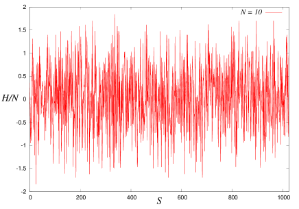
  Figure 1: Typical energy landscape $H(\bm{s})=-\sum_{i}J_{i}s_{i}s_{i+1}$ with $P(J_{i})=\mathcal{N}(0,1)$, $\mathbb{E}(J_{i}J_{j})=\delta_{i,j}$ of the spin glass chain. The number of spins is $N=10$. It should be noted that the horizontal axis $S$ denotes the label of states, that is, $S=1,2,\cdots,2^{N}(=1028)$. For instance, $S=1$ stands for a state, say, $\bm{s}(S=1)=(+1,+1,\cdots,+1)$ and $S=2^{N}$ denotes $\bm{s}(S=2^{N})=(-1,-1,\cdots,-1)$.

  We plot the typical energy landscape in Figure 1. From this figure, we find that the structure of the energy surface is complicated and it seems to be difficult for us to find the lowest energy state.

  However, we should notice that in (32) $s_{i}$ takes $\pm 1$ and the product $s_{i}s_{i+1}$ also has a value $\pm 1$. Hence, we introduce the new variable $\tau_{i}$ which is defined by $\tau_{i}=s_{i}s_{i+1}$, then $\tau_{i}$ takes $\tau_{i}\in\{1,-1\}$. Therefore, in order to minimize $H(\bm{\tau})=-\sum_{i}J_{i}\tau_{i}$, we should determine $\tau_{i}={\rm sgn}(J_{i})$ for each $i$ and then, we have the lowest energy as $U_{\rm min}=-\sum_{i}J_{i}\,{\rm sgn}(J_{i})=-\sum_{i}|J_{i}|$.

  

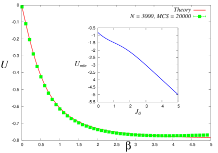
  Figure 2: Internal energy of spin glass chain as a function of temperature. The solid line is exact result $U=-\beta\int_{-\infty}^{\infty}\frac{Dx}{\cosh^{2}\beta x}$, whereas the dots denote the internal energy calculated by the MCMC for $N=3000$. The error-bars are calculated by $10$-independent runs for different choice of the $\{J\}\equiv\{J_{i}|i=1,\cdots,N\}$. The inset indicates the $U_{\rm min}$ as a function of $J_{0}$. We set $J=1$.

  Namely, when $J_{i}$ obeys a Gaussian with mean $J_{0}$ and variance $J^{2}$, the lowest energy for a single spin is obtained in the thermodynamic limit $N\to\infty$ as

  $$\lim_{N\to\infty}\frac{U_{\rm min}}{N} = \mathbb{E}_{\{J\}}(|J_{i}|)=\int_{-\infty}^{\infty}\frac{dJ_{i}}{\sqrt{2\pi}J}\,{\rm e}^{-\frac{(J_{i}-J_{0})^{2}}{2J^{2}}}|J_{i}|$$

  $$= -J_{0}-J\sqrt{\frac{2}{\pi}}\,{\rm e}^{-\frac{J_{0}^{2}}{2J^{2}}}$$

  where $\mathbb{E}_{\{J\}}(\cdots)$ here stands for the average over the configuration $\{J\}\equiv(J_{1},\cdots,J_{N})$.

  Thus, for the choice of $(J_{0},J)=(1,0)$, namely, in the limit of the ferromagnetic Ising model, we have the lowest energy as $U_{\rm min}/N=-1$ (all spins align in the same direction), On the other hand, for the choice of $(J_{0},J)=(0,1)$, we have $U_{\rm min}=-\sqrt{2/\pi}$. These facts mean that the lowest energy changes according to the value of ratio $J_{0}/J$.

  We next consider the case of finite temperature ($\beta<\infty$). For this case internal energy per spin is given by

  $$\lim_{N\to\infty}\frac{\langle H\rangle_{\tau}}{N}=\mathbb{E}_{\{J\}}(\langle H\rangle_{\tau})=-\frac{\partial}{\partial\beta}\log\sum_{\bm{\tau}}{\rm e}^{\beta\sum_{i}J_{i}\tau_{i}}$$ (33)

  with

  $$\langle\cdots\rangle_{\tau}\equiv\frac{\sum_{\bm{\tau}}{\exp}[\beta\sum_{i}J_{i}\tau_{i}]}{Z_{\tau}}$$ (34)

  where we defined

  $$\sum_{\bm{\tau}}(\cdots)\equiv\sum_{\tau_{i}=\pm 1}\cdots\sum_{\tau_{N}=\pm 1}(\cdots)$$ (35)

  and the partition function $Z_{\tau}=\sum_{\bm{\tau}}{\rm e}^{\beta\sum_{i}J_{i}\tau_{i}}$ is now calculated as $\{2\cosh(\beta J_{i})\}^{N}$. Hence, we have the average free energy density defined by $f=\lim_{N\to\infty}(\log Z/N)=N^{-1}\mathbb{E}_{\{J\}}(\log Z)$ is evaluated as follows (the self-averaging property we mentioned before was assumed).

  $$f = \int_{-\infty}^{\infty}\frac{dJ_{i}}{\sqrt{2\pi}\,J}{\rm e}^{-\frac{(J_{i}-J_{0})^{2}}{2J^{2}}}\log 2\cosh(\beta J_{i})$$ (36)

  $$= \int_{-\infty}^{\infty}Dx\log 2\cosh\beta(J_{0}+Jx)$$

  where we defined $Dx\equiv dx\,{\rm e}^{-x^{2}/2}/\sqrt{2\pi}$. From the above result, we immediately obtain the internal energy per spin $U=-{\partial f}/{\partial\beta}$ by

  $$U = -J_{0}\int_{-\infty}^{\infty}Dx\tanh\beta(J_{0}+Jx)$$ (37)

  $$- \beta J^{2}\int_{-\infty}^{\infty}\frac{Dx}{\cosh^{2}\beta(J_{0}+Jx)}.$$

  Especially, for the case of $(J_{0},J)=(0,1)$, we have

  $$U=-\beta\int_{-\infty}^{\infty}\frac{Dx}{\cosh^{2}\beta x}.$$ (38)

  In Figure 2, we show the $U$ as a function of $T$. From the arguments we provided above, we have the following learning equation (39) for the spin glass chain whose Hamiltonian is given by (32) is now rewritten as

  $$\frac{dT}{dt} = T^{2}\lim_{L\to\infty}\frac{1}{L}\sum_{l=1}^{L}\left(\sum_{i}J_{i}s_{i}(t,l)s_{i+1}(t,l)\right)$$ (39)

  $$- T\int_{-\infty}^{\infty}\frac{Dx}{\cosh^{2}T^{-1}x}.$$

• Sherrington-Kirkpatrick model
  This model is a spin glass model in which each spin is located on a complete graph. For this model, the energy function is explicitly given by

  $$H=-\frac{1}{N}\sum_{i=1}^{N}\sum_{j\neq i}J_{ij}s_{i}s_{j}$$ (40)

  where $J_{ij}$ obeys $P(J_{ij})={\cal N}(J_{0},J^{2})$.

  

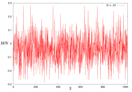
  Figure 3: Typical energy landscape $H(\bm{s})=-\sum_{ij}J_{ij}s_{i}s_{j}$ with $P(J_{ij})=\mathcal{N}(0,1)$, $\mathbb{E}(J_{ij}J_{kl})=\delta_{i,k}\delta_{j,l}$ of the SK model. The number of spins is $N=10$. It should be noted that the horizontal axis $S$ denotes the label of states, that is, $S=1,2,\cdots,2^{N}(=1028)$. For instance, $S=1$ stands for a state, say, $\bm{s}(S=1)=(+1,+1,\cdots,+1)$ and $S=2^{N}$ denotes $\bm{s}(S=2^{N})=(-1,-1,\cdots,-1)$.

  We plot the typical energy landscape in Figure 3. At first glance, it seems that the structure of energy surface is very similar to that of the spin glass chain, however, finding the lowest energy state of the SK model needs much more difficult tasks. This ‘ground state problem’ in the SK model is one of the non-trivial issues in the research field of spin glasses.

  By using the replica method we mentioned in the previous section, the averaged internal energy per spin, namely, the second term appearing in the learning equation (39) is calculated as

  $$\frac{U}{N}\equiv U_{\beta}(m,q)=-\frac{J_{0}}{2}m^{2}-\frac{\beta J^{2}}{2}(1-q^{2})$$ (41)

  where, $m,q$ are the replica symmetric solution for the magnetization and the spin glass order parameter, respectively. These are explicitly given by the following equations of state

  $$m\equiv\frac{1}{N}\sum_{i}\mathbb{E}_{\{J\}}(\langle s_{i}\rangle)=\int_{-\infty}^{\infty}Dz\,\tanh\beta(Jz\sqrt{q}+J_{0}m)$$ (42)

  $$q\equiv\frac{1}{N}\sum_{i}\mathbb{E}_{\{J\}}(\langle s_{i}\rangle^{2})=\int_{-\infty}^{\infty}Dz\,\tanh^{2}\beta(Jz\sqrt{q}+J_{0}m)$$ (43)

  where we defined

  $$\langle\cdots\rangle\equiv\frac{\sum_{\bm{s}}(\cdots){\exp}[(\beta/N)\sum_{ij}s_{i}s_{j}]}{\sum_{\bm{s}}{\exp}[(\beta/N)\sum_{ij}s_{i}s_{j}]}$$ (44)

  and $\mathbb{E}_{\{J\}}(\cdots)$ by (21). For these solutions for a given temperature $T$, the learning equation for the SK model is obtained by

  $$\frac{dT}{dt} = T^{2}\lim_{L\to\infty}\frac{1}{NL}\sum_{l=1}^{L}\left(\sum_{i}\frac{J_{ij}}{N}s_{i}(t,l)s_{j}(t,l)\right)$$ (45)

  $$- T^{2}U_{\beta}(m(T),q(T)).$$

  Here we should keep in mind that in the limit of $\beta\to\infty$, $\tanh\beta(\cdots)={\rm sgn}(\cdots)$, $q=1$ is derived from (43).

  On the other hand, from (42), the magnetization $m$ leads to

  $$m=\int_{-\infty}^{\infty}Dz\,{\rm sgn}(Jz+J_{0}m)=1-2\,{\rm erfcc}\left(\frac{J_{0}}{J}m\right)$$ (46)

  where we defined ${\rm erfcc}(x)$ by

  $${\rm erfcc}(x)\equiv\int_{x}^{\infty}\frac{dz}{\sqrt{2\pi}}\,{\rm e}^{-\frac{z^{2}}{2}}.$$ (47)

  By utilizing the asymptotic form $2\,{\rm erfcc}(x)\simeq 1-x\sqrt{2/\pi}$ around $x\simeq 0$, we obtain the critical point $a\equiv\sqrt{2/\pi}\,(J_{0}/J)=1$ below which the spin glass phase emerges. Hence, the lowest energy at zero temperature is obtained by substituting the solution $m$ of (46) into the expression of internal energy (41) with $q=1$, namely, $U/N=-J_{0}m^{2}/2$. As a special case, the lowest energy in the ferromagnetic state $J_{0}/J\to\infty$ is given by $U/J_{0}N=-1/2$. In Figure 4, we plot the internal energies per spin scaled as $\sqrt{2/\pi}\,(U/JN)=-am^{2}/2$ and $U/J_{0}N=-m^{2}/2$ and magnetization $m$ as a function of $a$ ($\equiv\sqrt{2/\pi}\,(J_{0}/J)$) at $T=0$.

  

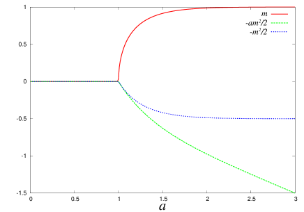
  Figure 4: Parameter $a$ ($\equiv\sqrt{2/\pi}\,(J_{0}/J)$)-dependence of magnetization $m$, internal energies per spin scaled as $\sqrt{2/\pi}(U/JN)=-am^{2}/2$ and $U/J_{0}N=-m^{2}/2$.

For these two mathematically tractable models, we shall evaluate the learning equations for effective Gibbs distributions in the next section.

5 Set-up for numerical experiments

For these two kinds of the solvable spin glass models, we examine the learning equations (39)(45) through the time-dependence of the effective temperature $T$ D In following, we explain our setting of parameters which control simple GA to be utilized in the learning processes.

• The number of spins $N$
  This is the number of components in a single gene configuration and is regarded as the number of spins in the spin glass model. Here we set $N=2000$ for spin glass chain and $N=500$ for the SK model.

• The number of ensembles (population) $M$
  The number of population in GA. We set $M=100$

• Parameters appearing in GA

  • $\sigma$: The number of members in selection of tournament -type at each generation.

  • $p_{c}$: The rate for a single point crossover

  • $p_{m}$: The mutation rate

• Effective temperature $T$
  A control parameter of the Gibbs distribution to approximate the empirical distribution of GA. We set the initial value $T=T_{0}\,(<\infty)$ D

• On the selection
  In our numerical experiments, we generate the configurations (members) with length $N$ randomly and for each of the member, we evaluate the fitness values. Then, we pick up $\sigma$ members among the population (ensemble) with size $M$ and select the largest fitness member and the others are discarded. We repeat the process up to $M$ times.

  As another candidate of selection, we might use the method to weight each member $\alpha$ of population with $p_{\alpha}={\rm e}^{-\beta_{s}E_{\alpha}}/\sum_{\alpha=1}^{M}{\rm e}^{-\beta_{s}E_{\alpha}}$ (see e.g. [Prugel-Bennett and L.Shapiro, 1994, Prugel-Bennett and L.Shapiro, 1997]). Obviously, $\beta_{s}\to\infty$ limit yields the case in which only the best solution is selected. Hence, the case $\sigma=M$ for our selection rule is identical to the $\beta_{s}\to\infty$ limit. On the other hand, $\beta_{s}=0$ limit corresponds to $\sigma=1$, namely, each member is selected randomly.

6 Results of numerical experiments

According to the set-up explained in the previous section, we shall carry out the numerical experiments for two mathematically tractable models. The results are summed up below.

6.1 Spin glass chain

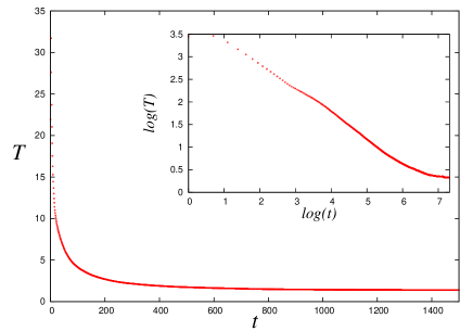
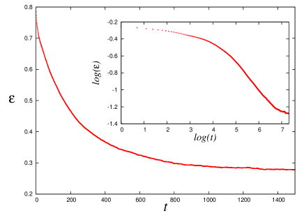
We first show the time-evolution of effective temperature and the residual energy for the case of spin glass chain with parameter sets: $\sigma=2,p_{c}=0.1,p_{m}=0.001$ in Figure 5. From this figure, we find that the asymptotic behaviour of the effective temperature follows a power-law. This schedule is faster than the effective temperature scheduling for the optimal simulated annealing $\sim 1/\log(1+t)$, however, slower than the exponential decreasing. Thus, here we define the residual energy and its time-dependence as the difference between the lowest energy and current energy obtained by the GA dynamics. We find that the residual energy which is defined by

$$\varepsilon\equiv H(\bm{s})-\min_{\bm{s}}H(\bm{s})$$ (48)

also asymptotically goes to zero and it follows a power-law in the scaling regime $t\gg 1$.

Figure 5: Time evolution of the effective temperature (upper panel) and the residual energy defined by (48) (lower panel) for the case of spin glass chain. We used a simple GA having $\sigma=2,p_{c}=0.1,p_{m}=0.001$. The inset stands for the asymptotic behaviour.

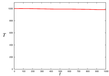
To investigate the effect of the selection operator on the GA dynamics, we carry out the same numerical experiments for the case of $\sigma=1$, namely, we investigate the time-evolution of the effective temperature for the GA without any effective selection (leading up to ‘random selection’). We plot the result in Figure 6. From this figure, we find that the effective temperature does not decrease and remains the same value as the initial condition. This means that the behaviour of the effective temperature is strongly dependent on the selection D

Figure 6: Time evolution of the effective temperature for the case of spin glass chain by simple GA having $p_{c}=0.1,p_{m}=0.001$ and without any selection operation $\sigma=1$.

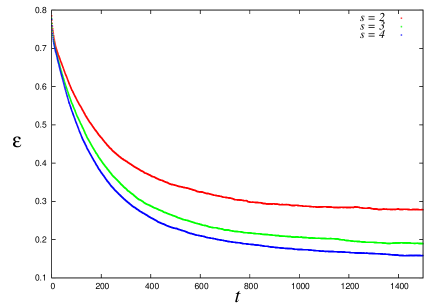
We next consider the relationship between the time-evolution of effective temperature, residual energy and the values of parameters for GA operations during the dynamics. We first fix $p_{c}=0.1,p_{m}=0.001$ and evaluate the result by changing the parameter $\sigma$ as $\sigma=2,3$ and $4$. The result is shown in Figure 7. From these panels, we find that the speed of effective temperature decreasing for large $\sigma$ value is faster than the result for small $\sigma$ value. However, in the asymptotic regime, the behaviour of effective temperature is almost independent of the choice of $\sigma$ value D

Figure 7: Time evolution of effective temperature and residual energy defined by (48) for the case of spin glass chain. We used a simple GA specified by $\sigma=2,3,4$ keeping $p_{c}=0.1$ and $p_{m}=0.001$.

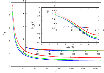
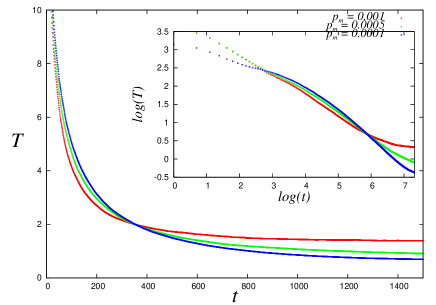
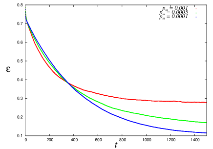
We next consider the case of $p_{m}=0.0001,0.0005$ and $0.001$ keeping $\sigma=2$ and $p_{c}=0.1$. The result is shown in Figure 8. From this figure, we confirm that the speed of convergence becomes very slow for both initial stage and asymptotic regime of the dynamics for $p_{m}=0.001$. This result implies that ‘mixing’ among the gene configurations is enhanced for large $p_{m}$ so as to prevent the Gibbs distribution from converging. On the other hand, for the case of $p_{m}=0.0005$ in the asymptotic regime, the speed of convergence is not so slow although the speed in the initial stage is actually slow. We also find this result from the behaviour of the residual energy. The result for $p_{m}=0.0001$ gives the largest exponent $\xi$ of the asymptotic form

$$T(t)=t^{-\xi},\,\,\,(t\gg 1),$$ (49)

namely, the speed of convergence is the fastest among the three cases D From the observation above, we find that mutation in a simple GA makes the population diverse to prevent us from trapping in a local minima of energy function and one can enhanced the speed of convergence asymptotically by setting the parameter $p_{m}$ to an appropriate value.

Figure 8: Time evolution of the effective temperature (upper panel) and the residual energy defined by (48) (lower panel) for the case of spin glass chain. We utilized a simple GA having $p_{m}=0.0005,0.001$ and $0.005$ keeping $p_{c}=0.1$ and $\sigma=2$.

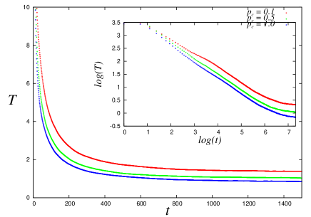
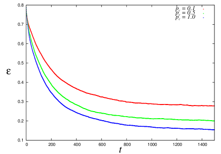
Finally, we investigate the time-evolution of effective temperature for $p_{c}=1.0,0.5$ and $0.1$ keeping $\sigma=2$ and $p_{m}=0.001$. The result is shown in Figure 9. From this figure, we find that higher value of the crossover rate gives higher convergence of the effective temperature. Generally speaking, a crossover is one of the essential operators in GA to generate genes having good quality in terms of minimization of the cost. However, at the same time, one has some risks to destruct the good equality gene itself when we choose too large crossover rate. The cost function we deal with in this section is that of the spin glass chain and interactions among the spins exist only in the nearest neighboring spin pairs. This fact means that there is less possibility that the crossover deconstructs the fine genes in comparison with the case of the Sherrington-Kirkpatrick model which will be mentioned in the next subsection. Actually, for the case of $p_{c}=1.0$, the GA gives the best performance among the three cases $p_{c}=1.0,0.5$ and $0.1$. Nevertheless, in the asymptotic regime, the three cases gives almost the same performance.

Figure 9: Time evolution of the effective temperature (upper panel) and the residual energy defined by (48) (lower panel) for the case of spin glass chain. We utilized a simple GA specified by $p_{c}=1,0.5,0.1$ keeping $p_{m}=0.001$ and $\sigma=2$.

6.2 Sherrington-Kirkpatrick model

We next consider the case of the SK spin glass. In the SK model, it is difficult for us to obtain the exact lowest energy to evaluate the residual energy. Hence, here we investigate the time evolution of effective temperature and the average fitness which is defined as negative internal energy $-U=-H(\bm{s})$.

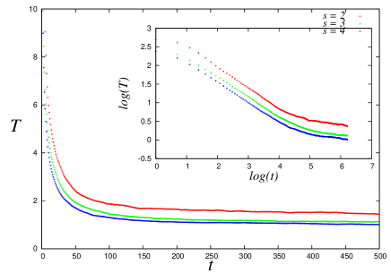
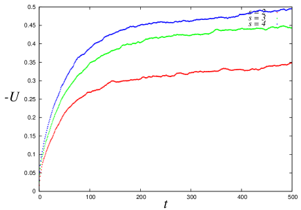
As we discussed in the previous subsection, we first investigate the time-evolution of these two physical quantities for the case of $\sigma=2,3$ and $4$ keeping $p_{c}=0.05,p_{m}=0.005$. We show the result in Figure 10. From these panels, we find that the asymptotic performance through the effective temperature does not change even if we increases the $\sigma$ value. However, it should be noticed that some ‘crossover phenomena’ takes place in some generation (time) regime. Namely, in this generation regime, the exponent $\xi$ in a power-law changes to the different exponent $\xi^{{}^{\prime}}$ ($>\xi$). On the other hand, at the beginning of the evolution, the average fitness value increases as the $\sigma$ value increases.

Figure 10: Time evolution of the effective temperature (upper panel) and the averaged fitness which is defined as negative internal energy $-U$ (lower panel) for the case of SK model. We used a simple GA having $\sigma=2,3$ and $4$ keeping $p_{m}=0.005$ and $p_{c}=0.05$. In the asymptotic regime $t\gg 1$ of time-evolution of temperature, ‘crossover phenomena’ are observed. Namely, the power-law exponent $\xi$ changes to the different value at intermediate time scale $\log t\sim 5$.

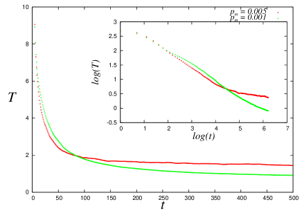
We next consider the case of $p_{m}=0.005,0.001$ keeping $s=2$ and $p_{c}=0.05$. The results are shown in Figure 11. From this figure, we confirm that the speed of convergence for the case of $p_{m}=0.005$ slows down in the asymptotic regime whereas the speed for the case of $p_{m}=0.001$ remains. The same behaviour as time evolution of the effective temperature is observed in the lower panel of Figure 11.

Figure 11: Time evolution of the effective temperature (upper panel) and the averaged fitness which is defined as negative internal energy $-U$ (lower panel) for the case of SK model. We used a simple GA having $p_{m}=0.005,0.001$ keeping $p_{c}=0.05$ and $\sigma=2$. In the asymptotic regime $t\gg 1$ of time-evolution of temperature for $p_{m}=0.005$, ‘crossover phenomena’ are observed. Namely, the power-law exponent $\xi$ changes to the different value at intermediate time scale $\log t\sim 5$.

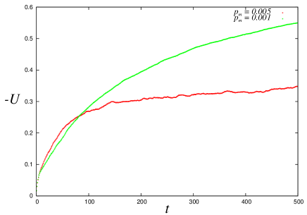
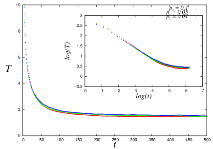
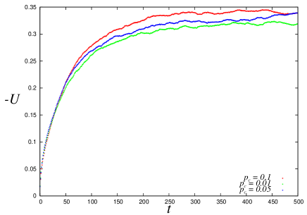
Finally, we shall show the results for $p_{c}=0.1,0.05$ and $0.01$ keeping $\sigma=2$ and $p_{m}=0.005$ in Figure 12. As the SK model is defined on a complete graph and all spins are connected, the crossover operation might destroy the gene configurations having relatively high fitness values. However, from the results shown in this figure, the average fitness value increases as the $p_{c}$ increases although the effective temperature does not change so much.

Figure 12: Time evolution of the effective temperature (upper panel) and the averaged fitness which is defined as negative internal energy $-U$ (lower panel) for the case of SK model. A simple GA having $p_{c}=0.1,0.05,0.01$ keeping $p_{m}=0.005$ and $\sigma=2$ is utilized.

7 Concluding remarks

In this paper, we introduced a learning algorithm of Gibbs distributions from training sets which are gene strings generated by GA to figure out the statistical properties of GA from the view point of thermodynamics. A procedure of average-case performance evaluation for genetic algorithms was numerically examined. The formulation was applied to the solvable probabilistic models having multi-valley energy landscapes, namely, the spin glass chain and the Sherrington-Kirkpatrick model. By using computer simulations, we discussed the asymptotic behaviour of the effective temperature scheduling and the residual energy induced by the GA dynamics.

Both effective temperature and residual energy show power-law behaviors given by (49), namely, $\beta_{t}=t^{\xi}$ for $t\gg 1$. In section 2, we showed that a Gibbs distribution with $\beta_{t}=t$ yields the Holland’s condition (8). Hence, it might be worth while for us to check to what extent the condition is modified for the Gibbs distribution with $\beta_{t}=t^{\xi}$. For this case, a Gibbs distribution with respect to the gene configuration having the fitness $g(i)$ is written as $p_{i}(t)={\exp}[t^{\xi}g(i)]/\sum_{j\in\mathcal{J}}{\exp}[t^{\xi}g(i)]$. Taking the derivative of the above equation with respect to $t$, we have $dp_{i}(t)/dt=\xi t^{\xi-1}\{p_{i}(t)g(i)-p_{i}(t)\sum_{j\in\mathcal{J}}g(i)p_{j}(t)\}$. Hence, by substituting this result into the equation obtained by taking the derivative of the probability $P(\mathcal{H},t)$ that a schema $\mathcal{H}$ appears, namely, $P(\mathcal{H},t)=\sum_{i\in\mathcal{H}}p_{i}(t)$ with respect to $t$, we obtained the modified Holland’s condition as ${dP(\mathcal{H},t)}/{dt}=\xi t^{\xi-1}\{f(\mathcal{H},t)-P(\mathcal{H},t)f(\mathcal{J},t)\}$. From this condition, we find that the temporal difference of the probability that the schema $\mathcal{H}$ appears increases by $\xi t^{\xi-1}$ for $\beta_{t}=\xi t^{\xi-1}$. More generally, we conclude that the temporal difference increases by $d\beta_{t}/dt$ for $\beta_{t}$.

Although we dealt with the average-case performance evaluation just for a simple GA, our general procedure given in this paper is apparently applicable to the other sophisticated GAs based on any population dynamics. Moreover, one can generalize the Gibbs form to be trained by Boltzmann-machine-type learning equation so as to include the so-called Tsallis distribution, which is specified by $\beta$ and $q$, as a special case [Nishimori and Inoue, 1998].

REFERENCES

- Baluja, 1994 Baluja, S. (1994). Population-based incremental learning: A method for integrating genetic search based function optimization and competitive learning. Technical Report, School of Computer Science, Carnegie Mellon University, CMU-CS-94:163.
- E.Goldberg, 1989 E.Goldberg, D. (1989). Genetic Algorithms in Search, Optimization and Machine Learninig. Addison-Wesley.
- Geman and Geman, 1984 Geman, S. and Geman, D. (1984). Stochastic relaxation, gibbs distributions, and the bayesian restoration of images. IEEE Trans. on Pattern Analysis and Machine Intelligence, PAMI-6:721–741.
- H.Chen and K.Ma, 1982 H.Chen, H. and K.Ma, S. (1982). Low-temperature behaviour of a one-dimensional ising model. Journal of Statsitcal Physics, 29:717–746.
- H.Holland, 1975 H.Holland, J. (1975). Adaptation in natural and artificial systems. The University of Michigan Press.
- Kirkpatrick et al., 1983 Kirkpatrick, S., D.Galatt, C., and P.Vecchi, M. (1983). Optimization by simulated annealing. Science, 220:671–680.
- Li, 1981 Li, T. (1981). Structure of metastable states in a random ising chain. Physical Review B, 24:6579–6587.
- L.Shapiro, 2005 L.Shapiro, J. (2005). Drift and scaling in estimation of distribution algorithms. Evolutionary Computation, 13.
- L.Shapiro, 2006 L.Shapiro, J. (2006). Diversity loss in general estimation of distibution algorithms. Lecture Notes in Computer Science, 4193.
- Mezard and Parisi, 1986 Mezard, M. and Parisi, G. (1986). A replica analysis of the travelling salesman problem. Journal de Physique, 47:1285–1296.
- Mezard et al., 1987 Mezard, M., Parisi, G., and Virasoro, M. (1987). Spin Glass Theory and Beyond. World Scientific, Singapore.
- Monasson et al., 1999 Monasson, R., Zecchina, R., Kirkpatrick, S., Selman, B., and Troyansky, L. (1999). Determining computational complexity from characteristic ‘phase transitions’. Nature, 400:133–137.
- Nishimori and Inoue, 1998 Nishimori, H. and Inoue, J. (1998). Convergence of simulated annealing using the generalized transition probability. Journal of Physics A: Mathematical and Genetal, 47:5561–5672.
- Pelikan et al., 1999 Pelikan, M., E.Goldberg, D., and E.Cantu-Paz, E. (1999). Boa: The bayesian optimization algorithm. In Proceedings of GECCO-99.
- Pelikan et al., 2000 Pelikan, M., E.Goldberg, D., and E.Cantu-Paz, E. (2000). Bayesian optimization algorithm, population sizing, and time to convergence. University of Illinois at Urbana-Champaign, Illinois Genetic Algorithms Laboratory, Urbana, IL, IlliGAL Report, No. 2000002.
- Pelikan et al., 2002 Pelikan, M., E.Goldberg, D., and G.Lobo, F. (2002). Survey of optimization by building and using probabilistic models. Computational Optimization and Applications, 21:5–20.
- Prugel-Bennett and L.Shapiro, 1994 Prugel-Bennett, A. and L.Shapiro, J. (1994). An analysis of genetic algorithms using statistical mechanics. Physical Review Letters, 72:1305–1309.
- Prugel-Bennett and L.Shapiro, 1997 Prugel-Bennett, A. and L.Shapiro, J. (1997). The dynamics of a genetic algorithm for simple ising systems. Physica D, 104:75–114.
- S.Correa and L.Shapiro, 2006 S.Correa, E. and L.Shapiro, J. (2006). Model complexity vs. performance in the bayesian optimization algorithm. Lecture Notes in Computer Science, 4193.
- Sherrington and Kirkpatrick, 1975 Sherrington, D. and Kirkpatrick, S. (1975). Solvable model of spin-glass. Physical Review Letters, 35:1792–1796.
- Suzuki, 1995 Suzuki, J. (1995). Markov chain analysis of simple genetic algorithm. IEEE Trans. on System, Man and Cybernatics, 25:655–659.
- Suzuki, 1998 Suzuki, J. (1998). A further result on the markov chain model od gas and their sa-like strategy. IEEE Trans. on System, Man and Cybernatics, 25:95–102.
- Suzuki, 2005 Suzuki, J. (2005). Statsitical physics approach to genetic algorithm (in japanese). In Proceedings of Computational Intelligence Seminar (8th November, 2005, Waseda University, Tokyo Japan).
- Talagrand, 2003 Talagrand, M. (2003). Spin Glasses: A Challenge for Mathematicians. Springer.