Difficulties in Complex Multiplication and Exponentiation

1 Introduction

Complex numbers create some of the most beautiful pictures in mathematics. Mandelbrot sets, Julia sets, and many other computer-generated images have become everyday images; hundreds of books have been published and songs have been written (my favorite is [9]). However, the algorithms which drive these computations make a major assumption about the complex plane which can create some visual havoc. Robert Corless ([3]) asked if there is a way to compensate for this error. Unfortunately, we show this is not possible.

2 Complex Multiplication and Exponentiation

The multiplication of two complex numbers is rather straight-forward: for $z_{1},z_{2}\in\mathbb{C}$, where $z_{1}=a+bi$ and $z_{2}=c+di$ with $a,b,c,d\in\mathbb{R}$ we have

$$z_{1}z_{2}=(a+bi)(c+di)=(ac-bd)+(ad+bc)i.$$ (2.1)

However, this is not computationally efficient for exponentiation; the computation of $(2+3i)^{3}$ is not as quick using this definition:

$$(2+3i)^{3}=(2+3i)(2+3i)(2+3i) = ((4-9)+(6+6)i)(2+3i)$$

$$= (-5+12i)(2+3i)$$

$$= (-10-36)+(-15+24)i$$

$$= -46+9i.$$

If we convert $2+3i$ to polar form $z=re^{i\theta}$, we can compute this exponential much faster. The conversion equations between rectangular coordinates $z=a+bi$ and polar form $z=re^{i\theta}$ are:

$$a=r\cos(\theta) b=r\sin(\theta)$$ (2.2)

$$r=\sqrt{a^{2}+b^{2}} \tan(\theta)=\frac{b}{a}$$ (2.3)

So we convert $2+3i$ to polar form: $r=\sqrt{2^{2}+3^{2}}=\sqrt{13}\approx 3.60555127\ldots$ and $\tan(\theta)=1.5\Rightarrow\theta\approx 0.9828$ or $56.31^{\circ}$. Now we can use some simple properties of exponents to get:

$$\left(re^{i\theta}\right)^{n}=r^{n}e^{in\theta}\textrm{ for }n\in\mathbb{N}$$ (2.4)

So we have

$$(2+3i)^{3}=\left(\sqrt{13}e^{0.9828i}\right)^{3}=\left(\sqrt{13}\right)^{3}e^{3(0.9828)i}\approx 46.87216658e^{2.94838117i}$$

Now convert this back into rectangular coordinates:

$$a = 46.87216658\cos(2.94838117)=-46$$

$$b = 46.87216658\sin(2.94838117)=9$$

so we have $(2+3i)^{3}=-46+9i$. Perhaps this polar form conversion seems more tedious, but consider how much easier it makes computations with higher powers, like $(2+3i)^{29}$ (which, in case you’re wondering, equals
$-13,833,225,534,613,558-3,190,610,873,034,597i$).

A closer examination of the complex exponential function reveals an interesting property: $e^{z}$ is not a one-to-one function! Using Equations 2.2 and 2.3, we see that the periodic nature of the trigonometric functions cause there to be multiple (co-terminal) angles which satisfy the formulae. For example, $1+i$ can be written as $\displaystyle{\sqrt{2\ }e^{\frac{\pi}{4}i}}$ and as $\displaystyle{\sqrt{2\ }e^{\frac{9\pi}{4}i}}$. The angles (referred to as the argument of the complex number; $\arg(z)$) differ by a multiple of $2\pi$, and any number of the form $\displaystyle{\sqrt{2\ }e^{(2k\pi+\frac{\pi}{4})i}}$ with $k\in\mathbb{Z}$ is also a polar form of $1+i$. This means that the inverse of the function $e^{z}$ is not a function, but we can work around this.

The standard definition of the logarithm of $z$ requires that we specify an interval of length $2\pi$ for the angles. This is called a branch of the logarithm. The generalized logarithmic function is defined by

$$\log(z)=\log(re^{i\theta})=\ln(r)+i\theta$$ (2.5)

Now we have a point where this function is undefined: when $z=0$ we would need to compute $\ln(0)$ and to find $\theta$, which is not well defined for 0. Any subset of the complex plane on which we can define a (one-to-one) function which acts as an inverse of $e^{z}$ is called a branch of the logarithm (see any introductory text of complex analysis for a more detailed exposition; like [2], pages 38-40). This requires that there is a part of the plane “removed” from the domain of $\log(z)$; this is called the branch cut. It is a curve from $z=0$ extending out to infinity; most often it is a straight line. When we us the principal branch of the logarithm, the cut is the non-positive real axis. This means that the angles used for $\theta$ are in the interval $(-\pi,\pi]$. This is the default branch in almost every computer algebra system in the world; and is called the principal branch of the logarithm. This means that $\log(z)$ is not analytic on the whole plane.

When we define $z^{n}=e^{n\log(z)}$ for $n\in\mathbb{N}$ we have a problem: how can the composition of nonanalytic functions become analytic? It has to do with the behavior of the branch cut. We will follow the computation through the following chain of compositions:

$$z\mapsto\log(z)\mapsto n\log(z)\mapsto e^{n\log(z)}=z^{n}$$ (2.6)

When we take a small disk $\Delta=\{z:|z-r|<\varepsilon\}$ about a point $r<0$ in the negative half of the real axis, it is divided into two halves by the axis (see Figure 1 on page 1):

$$\textrm{the upper half-disk }\Delta_{U} = \Delta\cap\{z|\operatorname{Im}(z)\geq 0\}$$

$$\textrm{the lower half-disk }\Delta_{L} = \Delta\cap\{z|\operatorname{Im}(z)<0\}$$

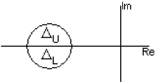
Figure 1: A disk on the negative real axis

These half-disks are transformed by the map $\log(z)$ into regions about the lines $\operatorname{Im}(z)=\pi$ and $\operatorname{Im}(z)=-\pi$. The images are almost semi-circular regions, with center at $\log(r)$ and radius of $\varepsilon$ (see Figure 2 on page 2).

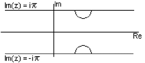
Figure 2: The image of the disk in Figure 1 under the map $\log(z)$

Now we have illustrated the first step in the chain in 2.6. Our next step is to multiply these points by $n\in\mathbb{N}$. This expands the entire picture; the horizontal edges of the half disks are moved to $\operatorname{Im}(z)=\pm n\pi$, and the radius will increase by a factor of $n$ as well. So we have the image as seen in Figure 3 on page 3. Our final step is to exponentiate; the result will depend on the parity of $n$. If $n$ is odd, the result is a disk of radius $\varepsilon^{n}$ centered around the point on the negative real axis with magnitude $r^{n}$ (i.e., the center is $-r^{n}$); if $n$ is even, the result is a disk of radius $\varepsilon^{n}$ centered around the point $r^{n}$ (the point on the positive real axis with magnitude $r^{n}$).

Figure 3: The image of the regions in Figure 2 multiplied by $n$

What is critical in this sequence of maps is the behavior of the half disks in Figure 3 when acted on by the exponential. When $n$ is an integer, these half disks are aligned after the exponential map: the arguments of the horizontal segments of the boundary are $n\pi$ and $-n\pi$ which are mapped to points on the real axis (see Figure 4 on page 4). When any other branch cut is used, the same process can be applied. The result is that the function defined by

$$z^{n}=\left\{\begin{array}[]{c l}e^{n\log(z)}&\ z\neq 0\\ 0&\ z=0\end{array}\right.$$ (2.7)

is analytic and well defined for $n\in\mathbb{N}$.

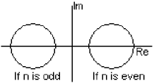
Figure 4: The image of the regions in Figure 3 under the map $e^{z}$

A technical aside: we can consider the infinite family of disks, with centers on the lines $\operatorname{Im}(z)=(2k+1)\pi,\ k\in\mathbb{Z},$ as the logarithmic image of the single disk in Figure 1. If we follow this line of reasoning, the expansion by a factor of $n$ is the critical step; all of the disks now have centers on lines with $\operatorname{Im}(z)=nk\pi,\ k\in\mathbb{Z}$, and the exponential will map this family of disks (in an infinite-to-one fashion) onto a single disk as seen in Figure 4 on page 4.

3 Non-integer Exponents

What happens when we try to define $z^{\alpha}$ if $\alpha$ is not an integer? We have the same sequence of composition:

$$z\mapsto\log(z)\mapsto\alpha\log(z)\mapsto e^{\alpha\log(z)}=z^{\alpha}$$ (3.1)

but what breaks down?

Let us take a simple example: $z^{\frac{1}{n}}$ for $n\in\mathbb{N}$. The process we used for the integer exponents can be paralleled, but we must consider the infinite family of disks mentioned at the end of Section 2. When we multiply by $\alpha=\frac{1}{n}$ in the second step, we will compress $n$ of these disks to lie between the lines $\operatorname{Im}(z)=-\pi$ and $\operatorname{Im}(z)-\pi$. An example (with $\alpha=2$) is shown in Figure 5 on page 5. This results in two distinct square root, and $n$ distinct $n^{\textrm{th}}$ roots in general, for any non-zero complex number. Note that if $n$ is even, then none of the family of disks will map onto the lines $\operatorname{Im}(z)=\pm\pi$, and there will be no problem when we exponentiate. However if $n$ is odd, then there are images of the branch cut (the lines $\operatorname{Im}(z)=\pm n\pi$) which are compressed onto the lines $\operatorname{Im}(z)=\pm\pi$. This causes members of the family of disks to lie on the branch cut, exactly as in Figure 2. Thus when we exponentiate, these half-disks realign, and the resulting function is analytic (away from $z=0$).

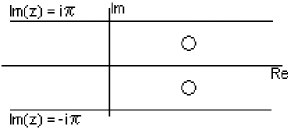
Figure 5: The images of the disk in Figure 1 under the map $\frac{1}{2}\log(z)$

However, the value $\alpha=\frac{1}{n}$ is a very special case. What about the more general case? The first step here works exactly as in Figure 2 on page 2; a disk about the negative real axis is split into two half-disks and mapped to two half-disks about the lines $\operatorname{Im}(z)=\pm\pi$. These regions are expanded by a factor of $\alpha$, so the lines in figure 3 on page 3 would be labelled $\alpha\pi i$ and $-\alpha\pi i$. When we restrict ourselves to the images contained between the lines $\operatorname{Im}(z)=\pm\pi$, we have something similar to that seen in figure 6 on page 6. Notice that the disks that intersect the branch cut lines are not bisected, but are divided into nonequal portions; this is a critical difference.

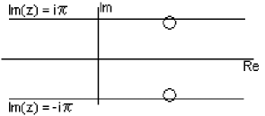
Figure 6: The images of the disk in Figure 1 under the map $\alpha\log(z)$

Now we exponentiate, and here is the rub: The images of the rays
$\operatorname{Im}(z)=\pm\alpha\pi$ do not coincide when $\alpha$ is not an integer! Depending on the value of $\alpha$, the result is similar to that seen in figure 7 on 7. This causes the function $f(z)=z^{\alpha}$ not to be analytic on the whole plane; it is not analytic at the center of our disk, $z=-r$. To be technical again, we should omit the branch cut from the domain of the function and say that the function is only analytic on the region $\mathbb{C}\setminus(\mathbb{R}^{-}\cup\{0\})=\mathbb{C}\setminus\{z:\operatorname{Re}(z)\leq 0,\operatorname{Im}(z)=0\}$.

Figure 7: The image of the disk from Figure 1 under the sequence of maps in Equation 3.1 on page 3.1

However, another definition of an analytic function is a function which is continuously differentiable on a region $G$, and $\frac{\textrm{d}}{\textrm{d}z}(z^{\alpha})=\alpha z^{\alpha-1}$, so clearly the function is differentiable. However, we must be careful with our choice of arguments (angles) to insure that the function is continuously differentiable. We will run into the same argument problem as in the definition of the logarithm, so we must make a branch cut, leading us to the same domain of analyticity mentioned in the previous paragraph.

How can we adjust the definition of $z^{\alpha}$ to create a function that possesses this continuous differentiability? We would like to arrange the branch cut so that when we follow the steps in Equation 3.1 the branch cuts align after the exponentiation. Let us examine a formula for generating the values of $z^{\alpha}$ and see how to address this problem.

4 Computation and Formulae

Computationally, what can we say about $z^{\alpha}$? How many distinct values in the complex plane should result? When $\alpha=\frac{1}{n}$, we have a direct formula for the $n^{\textrm{th}}$ roots $z^{\frac{1}{n}}=z^{\alpha}$ (see [2], for example):

$$z^{\frac{1}{n}}=|z|^{\frac{1}{n}}e^{\left(\frac{\theta+2k\pi}{n}\right)i}\quad\textrm{where }\theta=\arg(z),\ 0\leq k\leq n-1$$ (4.1)

which takes on $n$ distinct values in the complex plane. So if we were to extend this to non-integer values for $n$, we would have an equation for a non-integral root of $z$:

$$z^{\frac{1}{\eta}}=|z|^{\frac{1}{\eta}}e^{\left(\frac{\theta+2k\pi}{\eta}\right)i}\quad\textrm{where }\theta=\arg(z)$$ (4.2)

But how many values can $k$ range over? Without loss of generality, let $\eta=\frac{q}{p}$ with $(p,q)=1$. Then we can interpret Equation 4.2 as

$$z^{\frac{1}{\eta}}=z^{\frac{p}{q}}=|z|^{\frac{p}{q}}e^{\left(\frac{(\theta+2k\pi)p}{q}\right)i}\quad\textrm{where }\theta=\arg(z),\ 0\leq k\leq q-1$$ (4.3)

and we see that this formula will not cause the same value to appear until we have $q$ distinct values for $z^{\frac{p}{q}}$. This should make sense, since $z^{\frac{p}{q}}=\left(z^{p}\right)^{\frac{1}{q}}$. When we convert back to the rectangular coordinates, we see that these $q$ points are exactly the same as the $q$ points we compute using the $q^{\textrm{th}}$ roots of $z^{p}$, but they appear in a different order.

This formula (Equation 4.3) can be used to compute the $\alpha^{\textrm{th}}$ powers (where $\alpha=\frac{p}{q}$) of $z$ directly:

$$z^{\frac{p}{q}}=|z|^{\frac{p}{q}}e^{\left(\frac{(\theta+2k\pi)p}{q}\right)i}\quad\textrm{where }\theta=\arg(z),\ 0\leq k\leq q-1$$ (4.4)

However, this is not a one-to-one function; there are $q$ distinct values. These values have arguments that cover more that an interval of $2\pi$; in fact these $q$ values have arguments that range over the interval $[0,2q\pi)$! This is an important note and we will return to it after an example.

Example: Let us compute the $\frac{5}{2}^{\textrm{th}}$ powers of $1+i$. We will number them $r_{0},r_{1},\ldots,r_{4}$. We have $p=5,q=2,|1+i|=\sqrt{2},\theta=\frac{\pi}{4}$. So we can use Equation 4.4 and we get:

$$r_{k}=\left(\sqrt{2}\right)^{\frac{2}{5}}e^{\left(\frac{(\frac{\pi}{4}+2k\pi)2}{5}\right)i}\textrm{ where }0\leq k\leq 4$$

Now we evaluate this to get:

$$k=0 \Rightarrow r_{0}=\left(\sqrt{2}\right)^{\frac{2}{5}}e^{\left(\frac{(\frac{\pi}{4})2}{5}\right)i}=\left(\sqrt{2}\right)^{\frac{2}{5}}e^{\left(\frac{\pi}{10}\right)i}$$

$$k=1 \Rightarrow r_{1}=\left(\sqrt{2}\right)^{\frac{2}{5}}e^{\left(\frac{(\frac{\pi}{4}+2\pi)2}{5}\right)i}=\left(\sqrt{2}\right)^{\frac{2}{5}}e^{\left(\frac{9\pi}{10}\right)i}$$

$$k=2 \Rightarrow r_{2}=\left(\sqrt{2}\right)^{\frac{2}{5}}e^{\left(\frac{(\frac{\pi}{4}+4\pi)2}{5}\right)i}=\left(\sqrt{2}\right)^{\frac{2}{5}}e^{\left(\frac{17\pi}{10}\right)i}$$

$$k=3 \Rightarrow r_{3}=\left(\sqrt{2}\right)^{\frac{2}{5}}e^{\left(\frac{(\frac{\pi}{4}+6\pi)2}{5}\right)i}=\left(\sqrt{2}\right)^{\frac{2}{5}}e^{\left(\frac{25\pi}{10}\right)i}$$

$$k=4 \Rightarrow r_{4}=\left(\sqrt{2}\right)^{\frac{2}{5}}e^{\left(\frac{(\frac{\pi}{4}+8\pi)2}{5}\right)i}=\left(\sqrt{2}\right)^{\frac{2}{5}}e^{\left(\frac{33\pi}{10}\right)i}$$

Now compare this to the $5^{\textrm{th}}$ roots of $(1+i)^{2}=2i$, which we will denote $\rho_{0},\ldots,\rho_{4}$. We have $|2i|=2,\theta=\frac{\pi}{2},n=5$ so by Equation 4.1, we get:

$$\rho_{k}=|2|^{\frac{1}{5}}e^{\left(\frac{\frac{\pi}{2}+2k\pi}{5}\right)i},\textrm{ where }0\leq k\leq 4$$

which evaluates to the following:

$$k=0 \Rightarrow \rho_{0}=(2)^{\frac{1}{5}}e^{\left(\frac{\frac{\pi}{2}}{5}\right)i}=(2)^{\frac{1}{5}}e^{\left(\frac{\pi}{10}\right)i}$$

$$k=1 \Rightarrow \rho_{1}=(2)^{\frac{1}{5}}e^{\left(\frac{(\frac{\pi}{2}+2\pi)}{5}\right)i}=(2)^{\frac{1}{5}}e^{\left(\frac{\pi}{2}\right)i}$$

$$k=2 \Rightarrow \rho_{2}=(2)^{\frac{1}{5}}e^{\left(\frac{(\frac{\pi}{2}+4\pi)}{5}\right)i}=(2)^{\frac{1}{5}}e^{\left(\frac{9\pi}{10}\right)i}$$

$$k=3 \Rightarrow \rho_{3}=(2)^{\frac{1}{5}}e^{\left(\frac{(\frac{\pi}{2}+6\pi)}{5}\right)i}=(2)^{\frac{1}{5}}e^{\left(\frac{13\pi}{10}\right)i}$$

$$k=4 \Rightarrow \rho_{4}=(2)^{\frac{1}{5}}e^{\left(\frac{(\frac{\pi}{2}+8\pi)}{5}\right)i}=(2)^{\frac{1}{5}}e^{\left(\frac{17\pi}{10}\right)i}$$

We can see that there is a one-to-one correspondence between the values $r_{0},\ldots,r_{4}$ and the values $\rho_{0},\ldots,\rho_{4}$.

$$\rho_{0}= (2)^{\frac{1}{5}}e^{\left(\frac{\pi}{10}\right)i} =r_{0}$$

$$\rho_{1}= (2)^{\frac{1}{5}}e^{\left(\frac{\pi}{2}\right)i} =r_{3}\ \left(\textrm{since }\frac{25\pi}{10}\equiv\frac{\pi}{2}\pmod{2\pi}\right)$$

$$\rho_{2}= (2)^{\frac{1}{5}}e^{\left(\frac{9\pi}{10}\right)i} =r_{1}$$

$$\rho_{3}= (2)^{\frac{1}{5}}e^{\left(\frac{13\pi}{10}\right)i} =r_{4}\ \left(\textrm{since }\frac{33\pi}{10}\equiv\frac{13\pi}{10}\pmod{2\pi}\right)$$

$$\rho_{4}= (2)^{\frac{1}{5}}e^{\left(\frac{17\pi}{10}\right)i} =r_{2}$$

What we would like to develop is a way to avoid the branch cut problem seen in Figures 6 and 7 on page 7. We would like to arrange our domain so that the disks which cross the branch cut always realign (as in Figure 4 on page 4). This will require a new domain for the function $f(z)=z^{\alpha}$.

5 A New Domain?

For the function $z^{\alpha}+c=e^{(\alpha\log z)}+c$, with $\alpha=\frac{p}{q}$ a non-integral number, let us redefine the domain on a more general Riemann surface $W_{\alpha}$. (Note that this set could also be called $W_{q}$, but we want to emphasize the dependence on $\alpha$.) We construct the surface $W_{\alpha}$ by taking $q$ copies of the plane, all slit along the negative real axis, each identified by the branch of $\arg(z)$ used on each sheet. The sheet we label as the $0^{\textrm{th}}$ sheet has arguments in the interval $(-\pi,\pi]$, the sheet we label as the $+1^{\textrm{st}}$ sheet has arguments in $(\pi,3\pi]$, and so on up to the $(q-1)^{\textrm{st}}$ sheet, which has arguments in the interval $((2q-3)\pi,(2q-1)\pi]$. In general the $j^{\textrm{th}}$ sheet has arguments in the interval $((2j-1)\pi,(2j+1)\pi]$ for any integer $0\leq j<q$. The sheets are joined together at the negative real axis so that the argument is continuously rising as one travels in the positively oriented direction around the origin, and returning to the $0^{\textrm{th}}$ sheet after the $(q-1)^{\textrm{st}}$ sheet. In this fashion, the surface is similar to the Riemann surface for $z^{1/q}$ with its finite number of sheets. An example is seen in Figure 8 on page 8.

Figure 8: The surface $W_{\alpha}$

We must examine the definitions of multiplication and addition in order to define $F(z)=z^{\alpha}+c$ on this space properly. We must determine a method to keep track of the sheet we are on when we operate in this space.

5.1 Multiplying and Adding in our Domain.

Define $(z,m)\in(\mathbb{C},\mathbb{Z})$ as $z=re^{2\pi it}=re^{2\pi i(m+\xi)}$ where $t\in\left[m-\frac{1}{2},m+\frac{1}{2}\right)$. This assumes that the branch cut is the negative real axis. We define multiplication using the same idea as polar coordinates: given

$$z_{1}=r_{1}e^{2\pi it_{1}}=r_{1}e^{2\pi i(m_{1}+\xi_{1})}\qquad\textrm{ and }\qquad z_{2}=r_{2}e^{2\pi it_{2}}=r_{2}e^{2\pi i(m_{2}+\xi_{2})}$$

define

$$(z_{1},m_{1})(z_{2},m_{2})=(z_{1}z_{2},m_{*})=(r_{1}r_{2}e^{2\pi i(t_{1}+t_{2})},m_{*})\textrm{ where }t_{1}+t_{2}\in\left[m_{*}-\frac{1}{2},m_{*}+\frac{1}{2}\right)$$

Note that $m_{*}$ may or may not be equal to $m_{1}+m_{2}$; that depends on the values of $\xi_{1}$ and $\xi_{2}$. However, $m_{*}$ differs from $m_{1}+m_{2}$ by at most $\pm 1$. This allows us to define the non-integral powers of $(z,m)$ (i.e., $(z,m)^{\alpha}=(z^{\alpha},m_{*})$ for the appropriate value of $m_{*}$) in terms of the polar coordinates as well. In this context, keeping track of the sheet information is easy while multiplying.

This means that the Riemann surface $W_{\alpha}$ completely removes the branch cut discontinuities at 0 and $\infty$ established in the definition of $z^{\alpha}$. They are replaced by ramification points of $W_{\alpha}$; i.e., points where $z^{\alpha}$ is not locally one-to-one. So we have established a multiplication that works when $\alpha$ is not an integer.

However, when adding, keeping track of the sheet information is much harder. We want to define an addition operation (translation), called $\oplus$ to keep it straight, so that we can keep track of the sheet information our sum. So suppose that $(z,m_{1})\oplus(c,m_{2})=(w,m_{*})$, and we define the values of $w$ and $m_{*}$ as follows. Define $w$ as the usual sum of $z+c$ using rectangular coordinate addition.

We use the following cases to determine $m_{*}$; please note that QI is the first quadrant of the plane (i.e., the set $\{\operatorname{Re}(z)>0,\operatorname{Im}(z)\geq 0\}$ ), QII is the second quadrant (the set $\{\operatorname{Re}(z)\leq 0,\operatorname{Im}(z)\geq 0\}$), QIII the third quadrant ($\{\operatorname{Re}(z)\leq 0,\operatorname{Im}(z)<0\}$), and QIV is the fourth quadrant ($\{\operatorname{Re}(z)>0,\operatorname{Im}(z)<0\}$). Since we want our operation to agree with the exponentiation operation, we want the addition to be continuous in $\theta$, where $z=re^{i\theta}$. This is referred to as “Counter-Clockwise Continuity” or CCC in [4]. While this algorithm seems hard to follow, the idea is simple: if we cross the negative half of the real axis then we change sheets; if we cross from QII to QIII, then we go up one sheet, but if we cross from QIII to QII, then we go down one sheet.

Algorithm 5.1.1

To add the point $(c,0)$ to the point $(z,m)$ in $W_{\alpha}$, we choose the new sheet number $m_{*}$ as follows:

1. $\operatorname{Re}(c)=x_{c}=0$. There are three subcases:

   1. $\operatorname{Im}(c)=y_{c}=0$. Then $c=0$, $w=z$ and $m_{*}=m$ and we are done.

   2. $\operatorname{Im}(c)=y_{c}>0$. Then if $z$ is in QI, QII or QIV, we have
      $w=z+c$ in the sense of rectangular coordinate addition and $m_{*}=m$. However, if $z$ is in QIII, we have two further subcases:

      1. $|\operatorname{Im}(c)|\leq|\operatorname{Im}(z)|$. Then $m_{*}=m$

      2. $|\operatorname{Im}(c)|>|\operatorname{Im}(z)|$. Then $m_{*}=m-1$. Here is where we actually cross the branch cut.

   3. $\operatorname{Im}(c)=y_{c}<0$. Then if $z$ is in QI, QIII or QIV, we have $w=z+c$ in the rectangular coordinate sense and $m_{*}=m$. However, if $z$ is in QII, we have two further subcases:

      1. $|\operatorname{Im}(c)|<|\operatorname{Im}(z)|$. Then $m_{*}=m$.

      2. $|\operatorname{Im}(c)|\geq|\operatorname{Im}(z)|$. Then $m_{*}=m+1$. Here we cross the branch cut going the other way from the crossing above.

2. $\operatorname{Re}(c)=x_{c}>0$. Again we have three subcases

   1. $\operatorname{Im}(c)=y_{c}=0$. Then $m_{*}=m$ for any $z$.

   2. $\operatorname{Im}(c)=y_{c}>0$. If $z$ is in QI, QII, or QIV then $m_{*}=m$, but if $z$ is in QIII there are three subcases:

      1. If $|\operatorname{Im}(c)|\leq|\operatorname{Im}(z)|$ then $m_{*}=m$

      2. If $|\operatorname{Im}(c)|>|\operatorname{Im}(z)|$ and $|\operatorname{Re}(c)|\geq|\operatorname{Re}(z)|$ then $m_{*}=m$

      3. If $|\operatorname{Im}(c)|>|\operatorname{Im}(z)|$ and $|\operatorname{Re}(c)|<|\operatorname{Re}(z)|$ then $m_{*}=m-1$. This subcase, where $c$ moves $z$ up the imaginary axis, but not over far enough on the real axis to avoid the branch cut is the only one of these three subcases that crosses the branch cut.

   3. $\operatorname{Im}(c)=y_{c}<0$. If $z$ is in QI, QIII, or QIV, then $m_{*}=m$, but if $z$ is in QII there are three subcases:

      1. If $|\operatorname{Im}(c)|<|\operatorname{Im}(z)|$, then $m_{*}=m$

      2. If $|\operatorname{Im}(c)|\geq|\operatorname{Im}(z)|$ and $|\operatorname{Re}(c)|\geq|\operatorname{Re}(z)|$ then $m_{*}=m$

      3. If $|\operatorname{Im}(c)|\geq|\operatorname{Im}(z)|$ and $|\operatorname{Re}(c)|<|\operatorname{Re}(z)|$ then $m_{*}=m+1$.

3. $\operatorname{Re}(c)=x_{c}<0$. Here also, there are three subcases:

   1. $\operatorname{Im}(c)=y_{c}=0$. Then $m_{*}=m$ for any z.

   2. $\operatorname{Im}(c)=y_{c}>0$.

      1. If $z$ is in QI or QII, then $m_{*}=m$.

      2. If $z$ is in QIII, there are two possibilities: Either $|\operatorname{Im}(c)|\leq|\operatorname{Im}(z)|$ in which case $m_{*}=m$, or $|\operatorname{Im}(c)|>|\operatorname{Im}(z)|$ in which case $m_{*}=m-1$

      3. If $z$ is in QIV, there are three subcases

         1. If $|\operatorname{Re}(c)|\leq|\operatorname{Re}(z)|$ then $m_{*}=m$

         2. If $|\operatorname{Re}(c)|>|\operatorname{Re}(z)|$ and $|\operatorname{Im}(c)|\leq|\operatorname{Im}(z)|$ then $m_{*}=m$

         3. If $|\operatorname{Re}(c)|>|\operatorname{Re}(z)|$ and $|\operatorname{Im}(c)|>|\operatorname{Im}(z)|$ then $m_{*}=m-1$

   3. $\operatorname{Im}(c)=y_{c}<0$

      1. If $z$ is in QIII or QIV then $m_{*}=m$

      2. If $z$ is in QII the there are two possibilities: Either $|\operatorname{Im}(c)|<|\operatorname{Im}(z)|$ in which case $m_{*}=m$, or $|\operatorname{Im}(c)|\geq|\operatorname{Im}(z)|$ then $m_{*}=m+1$

      3. if $z$ is in QI, then there are three subcases:

         1. if $|\operatorname{Re}(c)|\leq|\operatorname{Re}(z)|$ then $m_{*}=m$

         2. if $|\operatorname{Re}(c)|>|\operatorname{Re}(z)|$ and $|\operatorname{Im}(c)|<|\operatorname{Im}(z)|$ then $m_{*}=m$

         3. if $|\operatorname{Re}(c)|>|\operatorname{Re}(z)|$ and $|\operatorname{Im}(c)|\geq|\operatorname{Im}(z)|$ then $m_{*}=m+1$

If we want to generalize to the case where we are adding $(z_{1},m_{1})$ and $(z_{2},m_{2})$, the process is nearly identical. We wish to preserve the idea from addition of vectors that the sum of two vectors lies “between” the vectors (i.e., the parallelogram law). The major change in the method above is that $m_{*}$ is now based on $\lfloor\frac{m_{1}+m_{2}}{2}\rfloor$ and then adjusted by $\pm 1$ depending on the cases above. The only main concern is that the point 0 is on every sheet. Hence if $z_{1}+z_{2}=0$ then the sheet is irrelevant. By default, the sheet should be left as $\lfloor\frac{m_{1}+m_{2}}{2}\rfloor$, in order to simplify the definition. This now allows us to add any two complex numbers in the Riemann surface setting. We will define neighborhoods of zero topologically: any ball of radius $\varepsilon$ around zero, covering all sheets, is a neighborhood of zero.

The major change is that addition is now a noncommutative operation! It is order dependent, as we see in the following example.

Example 1: Suppose we are working on a 4-sheeted space, like $W_{15/4}$. Let $(z_{1},m_{1})=(-2+i,2)$ and $(z_{2},m_{2})=(-1-3i,2)$. Converting these to polar coordinates, we get $z_{1}\approx\sqrt{5}e^{0.852416\pi i}$ and $z_{2}\approx\sqrt{10}e^{0.602416\pi i}$. So when we compute $(z_{1}+z_{2},m_{*})$ we get $z_{1}+z_{2}=-3-2i$ and $m_{*}=3$ (by case 3(c)(ii) above). However, when we compute $(z_{2}+z_{1},m_{*})$ we get $z_{2}+z_{1}=-3-2i$ and $m_{*}=2$ (by case 3(b)(ii) above). $\Box$

We run into a big problem: this operation is not continuous.

Counter-example 1: Let us consider an $\varepsilon$ -neighborhood $N$ of the point $z_{0}=(\frac{-i}{2},1)$, under the map $z\mapsto z+i$, on a three sheeted surface like $W_{\frac{8}{3}}$. Then when we translate, using Algorithm 5.1.1, the points in $N\cap\{\operatorname{Re}(z)<0\}$ are shifted to sheet 0, while the points in $N\cap\{\operatorname{Re}(z)\geq 0\}$ remain on sheet 1. Hence $N$ is “sheared” into two half-disks: one containing the point $(\frac{-i}{2},1)$, and one containing the point $(\frac{-i}{2},0)$ in its closure. $\Box$

This algorithm is specifically constructed to match the choice of the negative real axis as the branch cut. This is not the only way to construct the surface $W_{\alpha}$ and still maintain continuity in the argument, $t$, in our construction. We could use a branch cut along the positive real axis, or along any curve between the points 0 and $\infty$, just as any of these curves define a valid branch of the logarithm. But this will not change the continuity problem. In fact, any rigid translation on $W_{\alpha}$ is inherently discontinuous. Once we decide that our domain is a ramified Riemann surface like $W_{\alpha}$, translation becomes discontinuous at the ramification point (0 in our case).

Theorem 5.1.2

Let $C$ be the branch cut from 0 to $\infty$ of the surface $W_{\alpha}$. For any $c\in W_{\alpha}$, there exists a point $z_{0}$ and a neighborhood $N=N(z_{0})$ such that the set $N+c=\{z+c:z\in N\}$ is not a connected set (using a translation defined similarly to Algorithm 5.1.1, with $C$ as the branch cut). In particular, we may choose $z_{0}$ such that $0\in\{z_{0}+tc,\,0\leq t\leq 1\}$.

Proof: Fix $\alpha$ and $c$. Choose $z_{0}$ such that $0\in\{z_{0}+tc,\,0\leq t\leq 1\}$. Then the ray from the origin through $c$ divides $N=N(z_{0})$ into two subsets $N_{L}$ and $N_{U}$, each of which is a half-disk. When $N$ is translated, points in one of the half-disks change sheets, while points in the other half-disk do not change sheets. Regardless of which sheet the point $z_{0}$ is mapped onto, half of $N$ will be separated from $z_{0}$. If we approach $z_{0}$ in $N_{L}$, then for the sake of continuity, $z_{0}$ should be mapped onto the sheet containing $N_{L}$; but the same argument holds true for $N_{U}$. But the point $z_{0}$ is itself only mapped onto one sheet. Hence the translation map is not continuous. $\Box$

This answers a question raised by Robert Corless in his E.C.C.A.D. presentation [3]: “Can a Riemann surface variable be coded? What will the operations be on it?” (this was also discussed in detail in the Appendix A to E. Kaltofen’s paper [10].) Unfortunately, we are answering “No, a Riemann surface variable cannot be coded. There is no continuous addition operation on such a variable.”

We might also choose a different algorithm for choosing $m_{*}$. For example, we can define $m_{*}$ based on the sign of $\operatorname{Im}(c)$:

Algorithm 5.1.3

To add the point $(c,m_{2})$ to the point $(z,m_{1})$ in $W_{\alpha}$, we choose the new sheet number $m_{*}$ as follows:

1. If $\operatorname{Im}(c)>0$ then $m_{*}=m_{1}+m_{2}+1$.

2. If $\operatorname{Im}(c)=0$ then $m_{*}=m_{1}+m_{2}$.

3. If $\operatorname{Im}(c)<0$ then $m_{*}=m_{1}+m_{2}-1$.

But this algorithm for choosing sheets is not continuous either.

Counter-example 2: Fix $\alpha=\frac{5}{2}$ and $c=(i,0)$, so $W_{\alpha}$ has two sheets, with branch cut along the negative real axis. Consider an $\varepsilon$-neighborhood $N$ of the point $(-1,0)$. Now half of $N$ is on sheet 0 and half of $N$ is on sheet 1. Hence when we add $i$ using Algorithm 5.1.3, the neighborhood $N$ is “sheared” into two parts, since the points on sheet 1 are moved to sheet 0 and vice-versa. $N$ will become two half-disks centered about the points $(i,0)$ and $(i,1)$.

By defining the function $z^{\alpha}=e^{\alpha\log(z)}$ we have two points in $\overline{\mathbb{C}}$ where $F$ is not conformal, namely $0$ and $\infty$. This is caused by the branching of $\log(z)$ and the failure of the branch cuts to line back up after multiplying by $\alpha$ (recall the Figures 6 and 7). Any translation by $c$ cannot prevent these points from staying ramified. Hence ramification at zero implies either $c$ is also a ramification point or $z\mapsto z+c$ is not continuous. Since ramification at $c$ requires infinitely many ramification points (since $c$ is chosen arbitrarily), this isn’t a good plan.

6 Looking Forward

We come to the following negative result: the operation of addition is incompatible with the operation of exponentiation for non-integer exponents. So in order to study the fractals generated by functions of this form, we must redefine them on the plane and make sure that the definitions match the definitions for the integer case as closely as possible. We have examined these sets in a separate article ([13]).

Many of the characterizations of fractals for polynomials will fail to carry over to these functions and that the discontinuity we observed in Section 2 becomes more important than ever. This discontinuity is observed when an algorithm for generating fractals is given non-integer exponents. Figure 9, on page 9, is an example of the Julia set for the function $f(z)=z^{2.5}+\frac{1}{2}i$. This image was generated using the Fractint program (version 19.6) found at the web site given in [5] (using the fractal type julzpower), and the calculations were carried out using only the principal branch of the logarithm. The parameters for the julzpower fractal type are: the real and imaginary parts of the parameter ($0+0.5i$); the real and imaginary parts of the exponent ($2.5+0i$); the bailout test and the bailout value, both of which are set to 0 for the defaults (modulus for the test and 4 for the value).

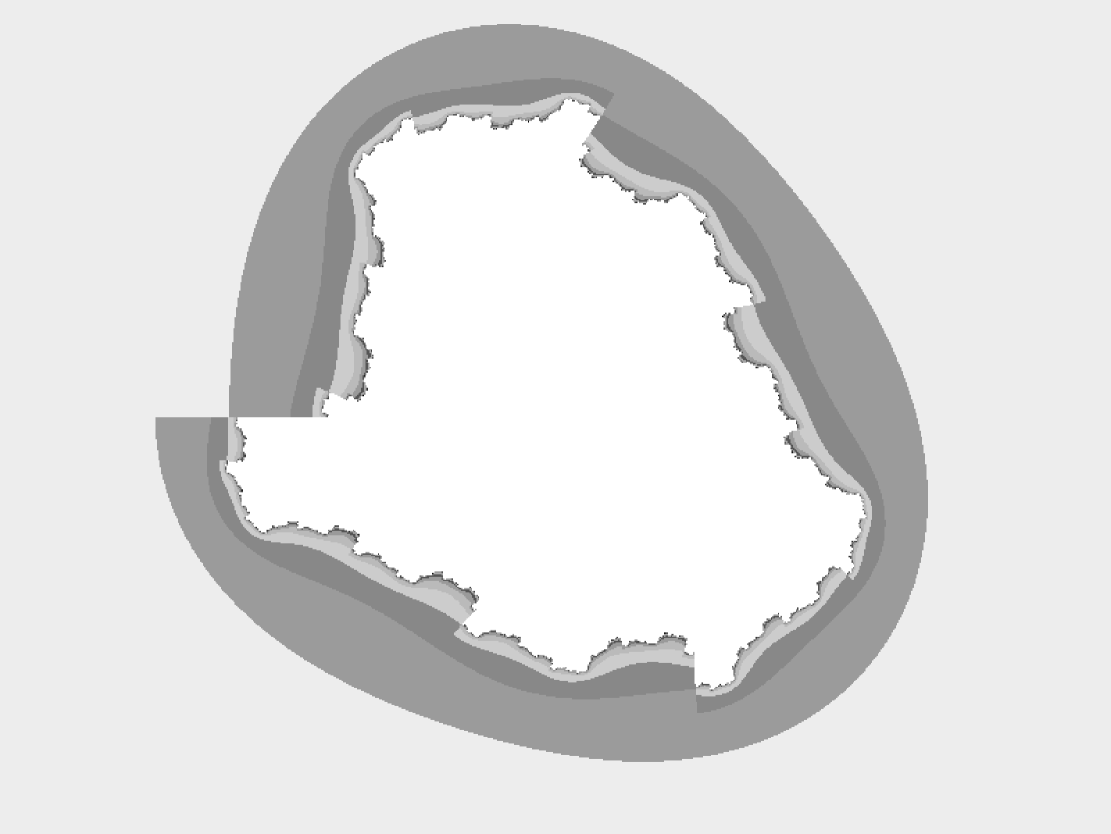
Figure 9: The Julia set for the function $f(z)=z^{2.5}+\frac{1}{2}i$

References

- [1] K. Becker and M. Dörfler: Dynamical systems and fractals, Computer experiments in Pascal, Cambridge University Press (1989)
- [2] J. Conway: Functions of One Complex Variable, second edition, Springer Verlag (1978)
- [3] R.M. Corless: Notes from “East Coast Computer Algebra Day 1998”, available on Dr. Corless’ web site at www.apmaths.uwo.ca/rcorless under the heading “Conferences”
- [4] R.M. Corless and D.J. Jeffrey: Editor’s Corner: The Unwinding Number, ACM SIGSAM Bulletin (Communications in Computer Algebra), v. 30, no. 1, issue 115, pages 28-35 (1996)
- [5] The Fractint Home Page, maintained by Tim Wegner, http://www.fractint.org
- [6] U. Gujar and V. Bhavsar: Fractals from in the Complex -Plane, Computers and Graphics, Volume 15, No. 3, pages 441-449 (1991)
- [7] U. Gujar, V. Bhavsar and N. Vangala: Fractal Images from in the Complex -Plane, Computers and Graphics, Volume 16, No. 1, pages 45-49 (1992)
- [8] E. F. Glynn: The evolution of the Gingerbread man, Computers and Graphics, volume 15, No. 4, pages 579-582 (1991)
- [9] J. Coulton: Mandelbrot Set, from the album Where Tradition Meets Tomorrow, ASIN: B000701FQQ, http://www.jonathancoulton.com/ (2004)
- [10] E. Kaltofen: Challenges of Symbolic Computation: My Favorite Open Problems, Journal of Symbolic Computation, Volume 29, pages 891-919 (2000)
- [11] A. Lakhtakia, V. V. Varadan, R. Messier and V. K. Varadan: On the symmetries of the Julia sets for the process , Journal of Physics. A. Mathematical and General, Volume 20, pages 3533-3535 (1987)
- [12] J. Sasmor: Fatou, Julia and Mandelbrot Sets For Functions With Non-Integer Exponent, Ph.D. Thesis, University of Pittsburgh, (2002)
- [13] J. Sasmor: Fractals for Functions with Rational Exponent, Computers and Graphics Elsevier, Vol. 28 No. 4, pages 601-615 (2004)