A comprehensive study of shower to shower fluctuations

Abstract

By means of Monte Carlo simulations of extensive air showers (EAS), we have performed a comprehensive study of the shower to shower fluctuations affecting the longitudinal and lateral development of EAS. We split the fluctuations into physical fluctuations and those induced by the thinning procedure customarily applied to simulate showers at EeV energies and above. We study the influence of thinning on the calculation of the shower to shower fluctuations in the simulations. For thinning levels larger than $R_{\rm thin}=10^{-5}-10^{-6}$, the determination of the shower to shower fluctuations is hampered by the artificial fluctuations induced by the thinning procedure. However, we show that shower to shower fluctuations can still be approximately estimated, and we provide expressions to calculate them. The influence of fluctuations of the depth of first interaction on the determination of shower to shower fluctuations is also addressed.

1 Introduction

Extensive air showers (EAS) have been studied over the last 70 years [1]. They result from the interaction in the atmosphere of high-energy protons and nuclei arriving from space. The product of these collisions are a set of secondary particles carrying a fraction of the primary energy. These secondaries move through the atmosphere and interact again generating new secondaries. The process continues, increasing the number of secondary particles, until their energies are too low to contribute to the generation of new particles. Particles reaching ground are sampled with arrays of detectors, and their properties are used to infer the properties of the primary initiating the shower. Measurements of the electron and muon density, of the arrival time of the particles at ground, and of the depth at which the shower has the maximum number of particles (X_max), give information on the arrival direction, primary energy, and on the mass of the primaries [1].

The complexity of the cascade phenomena, and the poor knowledge of the hadronic interactions at very high energy [2], make the experimental determination of the properties of the primaries very difficult. Moreover, primary particles with the same energy, mass and direction produce secondary particles with parameters that vary from shower to shower. This feature is called “shower to shower fluctuations”. An understanding of the shower to shower fluctuations will help to improve the interpretation of cosmic-ray data.

The calculation of shower to shower fluctuations can in principle be addressed with Monte Carlo simulations of extensive air showers. However, the number of particles that are produced in an air shower at ultra high energy (above $\sim 10^{18}$ eV) is so large ($\sim 10^{10}$), that it is almost impossible to follow the propagation to ground level of all the secondaries in the Monte Carlo in a reasonable amount of time, or even to store the large amount of information produced. For this reason, a statistical sampling procedure called “thinning” [3] is used in the simulations. Thinning algorithms typically consist on propagating only a small, representative fraction of the total number of particles in the shower, assigning statistical weights to the sampled particles to compensate for the rejected ones. However, thinning algorithms introduce artificial fluctuations in the simulated showers, hampering the determination of the intrinsic, physical shower to shower fluctuations with Monte Carlo simulations. For this reason the study of fluctuations using Monte Carlo simulations is quite difficult and uncertain. This is of utmost importance in cosmic-ray physics, since an incorrect assumption on the shower to shower fluctuations can lead to systematic errors on the determination of the parameters of the primary particles.

In this work we address the problem of determining the true, physical shower to shower fluctuations in Monte Carlo simulations, and quantify the effect of thinning on their determination. We give expressions that allow the estimation of physical fluctuations from Monte Carlo simulations, even in the case of relatively strongly thinned showers.

The paper is organized as follows: In Section 2 we describe the simulations performed in this work, and the thinning algorithm adopted. In Section 3 we identify the different sources of fluctuations in shower simulations. In Section 4 we perform a comprehensive study of the fluctuations in the longitudinal and lateral shower development, and give expressions that allow to separate physical shower to shower fluctuations from the artificial fluctuations induced by the thinning procedure. In Section 5, we quantify the influence on the shower to shower fluctuations of the fluctuations of the depth of first interaction of the primary initiating the shower. Finally, we summarize our conclusions in section 6. In the Appendix we give an explicit mathematical derivation of the expressions presented in Section 4.

2 The simulations

In this work we have used the air shower simulation program, AIRES [4, 5], along with the hadronic model QGSJET01 [6] to simulate proton and iron-induced showers with primary energy $10^{19}$ eV. As explained above, due to the large number of particles that are created in the simulation, AIRES includes a statistical sampling algorithm, that consists on propagating a small, representative fraction of the total number of particles, assigning a statistical weight $w$ to the sampled particles to compensate for the rejected ones. The weight is adjusted in such a way that both the total energy and the average number of particles is guaranteed to be conserved.

Before the simulation starts, the user indicates, as an input to AIRES, the relative thinning level $R_{\rm thin}$. The thinning energy $E_{\rm thin}$ - the energy below which the thinning process starts - is defined as $E_{\rm thin}$=$R_{\rm thin}\times E_{p}$ where, $E_{p}$ is the primary energy. For ultra high energy cosmic ray shower simulations convenient values for the relative thinning are $R_{\rm thin}=10^{-5}-10^{-9}$, but the actual choice depends on the purpose of the simulation. The thinning level affects both the simulation CPU time and the size of the output produced in the simulation, both typically behaving linearly with $R_{\rm thin}^{-1}$. If we increase $R_{\rm thin}$ by a factor of 10 the simulation speeds up by a similar factor, and the output is reduced accordingly, but the price to pay is an enhancement of the artifical fluctuations in the simulated showers as discussed below.

We describe here the thinning algorithm implemented in the AIRES code [5], originally due to Hillas [3]. At the beginning of the simulation, the primary particle is assigned a weight $w=1$. Then the primary is propagated and interacts in the atmosphere producing $n$ secondary particles. Before incorporating any secondary particle in the simulation, the energy of the primary $E_{p}$ which has generated that secondary is compared to $E_{\rm thin}$. If $E_{p}>E_{\rm thin}$, then all the secondaries with energy greater or equal than $E_{\rm thin}$ are kept, and their weight is equal to the weight of the primary particle. Secondaries with energy less than $E_{\rm thin}$ are kept with a probability $p_{i}=E_{i}/E_{\rm thin}$ ($E_{i}$ is the energy of $i^{\rm th}$ secondary), and their weight is adjusted so that $w_{i}=(1/p_{i})\times w$, with $w$ being the weight of the mother particle producing that secondary. On the other hand if $E_{p}<E_{\rm thin}$, it means that the particle came from a previous thinning operation. Then, one and only one of all the produced secondaries - say the $j^{\rm th}$ - is kept, with probability $p_{j}=E_{j}/\sum\limits_{i=1}^{n}E_{i}$. Again, the weight of this particle is increased by a factor $w_{j}=(1/p_{j})\times w$.

To avoid confusion between particles and weights, we identify an entry with a particle explicitely followed in the simulation which is associated a weight $w$. Hence, an entry represents $w$ particles. It is important to stress that once the thinning energy is reached, the number of entries $N_{e}$ is no longer increased in the shower processes (only one secondary particle is followed in each interaction), while the number of particles $N$ does however increase, since the weight of each entry typically increases in the showering process. When evaluating a physical observable, each entry must be weighted with its corresponding statistical weight.

In AIRES, the thinning algorithm is complemented with an “extended thinning algorithm” [5], designed to ensure that all the statistical weights are always smaller than a certain positive number (other algorithms based on this same idea are possible, see for instance [7]). To ensure this, an external parameter called statistical weight factor $W$ is available in the simulation. To further optimize the procedure of sampling, separated weight factors for electromagnetic ($W({\rm EM})$) and heavy particles ($W({\rm HADRONIC})$), are defined. The parameter $W({\rm HADRONIC})$ is specified indirectly by the ratio:

$${\rm AEH}=\frac{W({\rm EM})}{W({\rm HADRONIC})}.$$ (1)

The default value of this ratio in the simulation is ${\rm AEH}=88$. The default value of the weight factor $W({\rm EM})$ is 12. In this paper, we will use these default values unless otherwise specified.

We have simulated proton and iron-induced showers with primary energy $E_{p}=10^{19}$ eV, zenith angle $\theta=0^{\circ},\leavevmode\nobreak\ 30^{\circ},\leavevmode\nobreak\ 45^{\circ}$ and $60^{\circ}$ and relative thinning $R_{\rm thin}=10^{-5},\leavevmode\nobreak\ 10^{-6},\leavevmode\nobreak\ 10^{-7}$ and $10^{-8}$ (the two latter $R_{\rm thin}$ for proton only). We have also simulated showers with relative thinning of $R_{\rm thin}=10^{-7}$ but with $W({\rm EM})=0.1$ instead of the default value. Finally, we have also simulated two sets of proton and iron-induced showers at $\theta=0^{\circ}$, with fixed depth of first interaction, starting at the corresponding mean interaction depth for protons and iron at $10^{19}$ eV.

3 Fluctuations in EAS

In a real shower or in a simulation of an EAS, there are a number of different fluctuations that can occur. Rather generally, we can make a simple classification as shown in Table 1.

“Physical fluctuations” are those due to physical processes in the shower. Here we split them into those due to the first interaction, and those occuring in the secondary interactions, as is customary, and because it has recently been suggested that “universal” shower properties may emerge when considering only the fluctuations in the first interaction point [8]. Physical fluctuations occuring in the first interaction are further divided into those affecting the depth of the first interaction, and those that arise from fluctuations of multiplicity or inelasticity also in the first interaction.

Physical fluctuations	- Depth of first interaction.
	- Multiplicity, inelasticity, etc, in $1^{\rm st}$ interaction.
	- Secondary interactions.
Experimental fluctuations	- Detector response.
	- Sampling fluctuations.
Artificial fluctuations	- Thinning.
	- Un-thinning.

Table 1: Classification of the fluctuations in a shower, arising from the physical processes in the shower and the measurement process, and those that appear only in shower simulations.

In the case of real data, fluctuations are enlarged due to the detector response, and to the fact that the detector usually only samples a small fraction of the shower front. This “sampling fluctuation” is a statistically well known problem, and sampling fluctuations are rather well studied [9, 10]. We will not consider them in this work. Also the detector response introduces an additional source of fluctuations, which are detector dependent, and will not be considered here.

On the other hand, Monte Carlo simulated data is affected by artificial fluctuations due to the thinning and un-thinning (re-sampling) procedures. For the purposes of this work we do not need to consider the effect of fluctuations induced by the unthinning procedure [9].

4 Fluctuations of the longitudinal and lateral shower development

4.1 Fluctuations of the longitudinal profile

In Fig. 1 we show the average longitudinal profile of the number of electrons (left panels) and muons (right panels) $\bar{N}$, obtained in simulations of 100 proton-induced showers with $E_{p}=10^{19}$ eV, for thinning levels $R_{\rm thin}=10^{-6}$ and $10^{-7}$ and $\theta=0^{\circ},\leavevmode\nobreak\ 60^{\circ}$. Also shown are the relative shower to shower fluctuations $\sigma/\bar{N}$ for electrons and muons. As it is well known [11], the relative fluctuation has a minimum close to the depth of shower maximum. Also and as it is apparent from the figures, the dependence of the relative fluctuation on the thinning is small, at least for depths close to the depth of maximum.

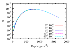
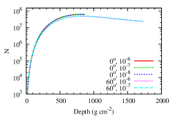
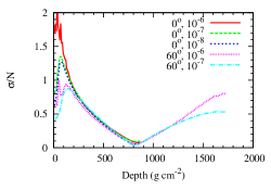
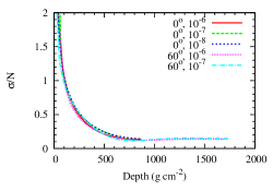
Figure 1: Upper panels: Longitudinal development of the average number of electrons (left) and muons (right) as a function of the slanted depth. Lower panels: Relative fluctuations $\sigma/\bar{N}$ as a function of the slant depth for electrons (left) and muons (right). In all panels: 100 proton-induced showers with $E_{p}=10^{19}$ eV and $\theta=0^{\circ}$ and $60^{\circ}$, were simulated with relative thinning $R_{\rm thin}=10^{-6}$, 10^-7 and 10^-8.

In Fig. 2 we show for the same showers in Fig. 1, the skewness and the kurtosis of the distribution of the number of particles $N$ at different depths. It is worth recalling that the skewness of the distribution of a variable $x$ is defined as

$$\gamma_{3}=\frac{\langle(x-\bar{x})^{3}\rangle}{\sigma_{x}^{3}},$$ (2)

where $\bar{x}$ ($\sigma_{x}$) is the average (standard deviation) of $x$. The kurtosis is defined as

$$\gamma_{4}=\frac{\langle(x-\bar{x})^{4}\rangle}{\sigma_{x}^{4}}-3.$$ (3)

where the “$-3$” in the definition is a convention to make $\gamma_{4}=0$ for a Gaussian distribution. Both the kurtosis and the skewness can be positive or negative. The skewness is a measure of the asymmetry of the distribution with respect to the mean value. A negative sign implies that the distribution is “deformed” towards values of $x$ smaller than the mean. The contrary applies for a positive sign. The kurtosis is a measure of the length of the tails of the distribution. Positive values imply that the distribution has tails longer than those of a Gaussian, while negative values imply that the tails are shorter (for instance a flat distribution, a box, has kurtosis -1.2). A Gaussian distribution has $\gamma_{3}=\gamma_{4}=0$.

Several remarks can be made from Fig. 2. Firstly, it is apparent that both, the skewness and the kurtosis of the distribution of the number of particles depend strongly on the thinning level, contrary to what happens to the mean $\bar{N}$ and to the relative fluctuations $\sigma/\bar{N}$. Close to the depth of shower maximum both the skewness and the kurtosis have local extrema very different from zero, implying that the distribution is strongly non-Gaussian. The skewness is negative and this implies that the distribution is asymmetric towards smaller values of $N$ than average. The positive values of the kurtosis imply that the distribution of $N$ has tails longer than those of a Gaussian, at least close to shower maximum. Remarkably, the log-Gaussian distribution, widely used to parameterize fluctuations in the number of electrons, has both $\gamma_{3}>0$ and $\gamma_{4}>0$, while the fluctuations predicted by Monte Carlo simulations near the maximum of the shower, have negative skewness. For muons and at large depths the skewness is close to zero, so that a Gaussian or a log-Gaussian distribution is a good approximation. For electrons, this is never the case.

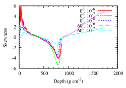
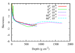
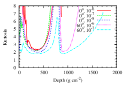
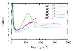
Figure 2: Upper panels: Skewness of the distribution of number of electrons (left) and muons (right) as a function of the slant depth. Lower panels: Same as the upper panels for the kurtosis. In all panels: 100 proton-induced showers of $E_{p}=10^{19}$ eV with $\theta=0^{\circ}$ and $60^{\circ}$ were simulated with relative thinning $R_{\rm th}=10^{-6}$, 10^-7 and $10^{-8}$.

4.2 Fluctuations of the lateral profile at ground

Of special importance for cosmic-ray physics performed with arrays of detectors is the study of fluctuations in the number of particles at ground.

In Fig. 3 we show the relative fluctuations ($\sigma/\bar{N}$) of the total number of electrons (left panels) and muons (right panels) at ground (upper panels), and in a ring of width $\Delta r$ at a distance $r=1000$ m from the shower axis (lower panels). In both cases the fluctuations are shown as a function of the number of showers simulated. The ring was taken from $r_{\rm min}=912$ m to $r_{\rm max}=1092$ m, i.e. $\Delta r=180$ m corresponding to a symmetric interval in the logarithm of $r$ around $r=1000$ m, chosen so that it compensates the decreasing density of particles with a larger area as $r$ increases.

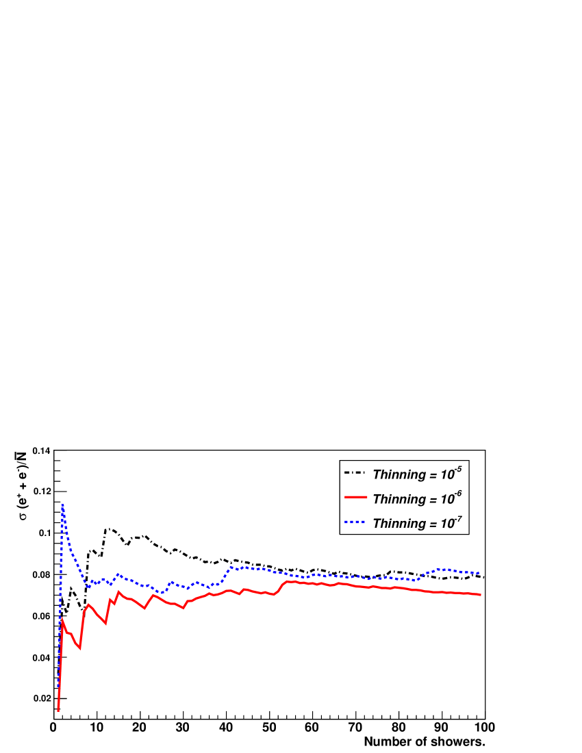
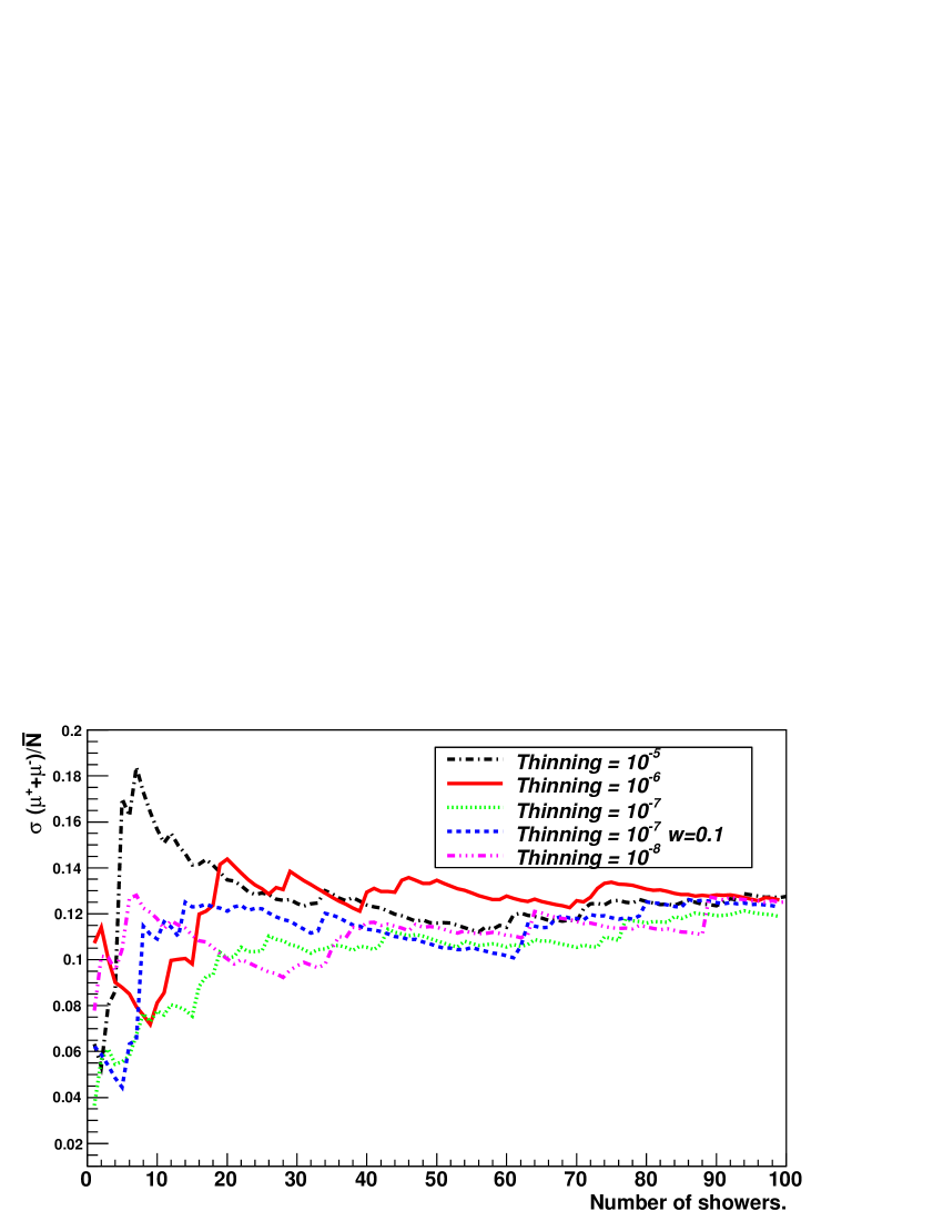
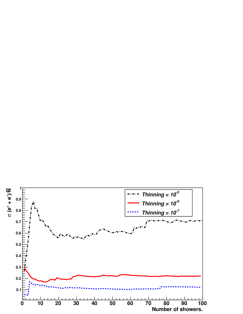
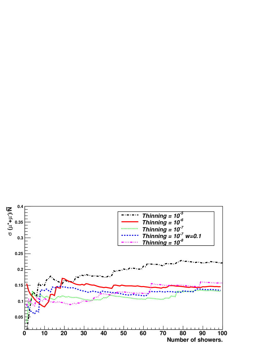
Figure 3: Relative fluctuations ($\sigma/\bar{N}$) in the number of electrons (left panels) and muons (right panels) versus the number of showers in the simulations. In the upper panels we show the relative fluctuation of the total number of particles at ground. In the lower panels we show the fluctuations of the number of particles falling in a ring $\Delta r$ at ground around a distance to the shower core $r=1000$ m. In all panels: proton-induced showers of energy $E_{p}=10^{19}$ eV and $\theta=0^{\circ}$ were simulated with relative thinning as indicated in the insets.

As expected, fluctuations in the ring $\Delta r$ are larger than the fluctuations in the whole ground. Also, the fluctuations in the ring have a stronger dependence with the thinning level used than those in the whole ground. This is easy to understand. An entry of weight $w$ falling in the ring represents $w$ particles, so that by losing or gaining just a single entry, one would lose or gain $w$ particles and the fluctuations are enlarged. This effect is not so strong when accounting for all the particles falling anywhere on the ground. In Fig. 3 it can also be clearly seen that no reliable evaluation of the fluctuations can be done with less than about 20 simulated showers, especially in the case of fluctuations in the ring. It can also be seen that a thinning level of $R_{\rm thin}=10^{-6}$ or larger, introduces large artificial fluctuations, so that the shower to shower physical fluctuations cannot be evaluated reliably. This is however no obstacle to approximately estimate the physical shower to shower fluctuations as will be shown in the following.

4.2.1 Physical shower to shower fluctuations at ground

In the Appendix we prove that the distribution of the number of particles $N$ as obtained in thinned Monte Carlo simulations of extensive air showers has a mean $\bar{N}$ and a standard deviation $\sigma$ given by:

$$\bar{N}=\bar{N}_{e}\;\bar{w},$$ (4)

and,

$$\sigma^{2}=\bar{N}_{e}\Omega^{2}+\bar{w}^{2}s^{2}.$$ (5)

where:

• $\bar{N}_{e}$ and $s$ are respectively the mean and the standard deviation of the distribution of the number of entries $N_{e}$ falling in a given ring around shower axis in each shower, i.e., the distribution of the number of non-thinned (explicitely sampled) particles in the simulation.

• $\bar{w}$ and $\Omega$ are respectively the mean and the standard deviation of the distribution of weights assigned to the entries.

Of course Eq. (4) is exact since the thinning algorithm is designed to reproduce it. For Eq. (5), the proof only assumes that the probability for an entry to have a given weight $w$ is independent of the probability of a shower to have a given number of entries $N_{e}$. This is only approximate since the total number of entries and their weights are constrained by energy conservation.

One can interpret Eq. (5) as follows. If all entries (sampled particles) had the same weight equal to $\bar{w}$ in all the simulated showers, then the distribution of weights would not fluctuate from shower to shower and we would get $\Omega=0$. In this limit we would obviously have $\sigma=\bar{w}s$. This special case of Eq. (5) was also found in [12]. In the particular case in which all weights are equal to $\bar{w}=1$, i.e. the shower is fully simulated and the thinning procedure is not applied, then clearly $N=N_{e}$, $\sigma=s$ and the fluctuations would be obviously dominated by the true, physical shower to shower fluctuations. In the opposite limit, if we imagine that showers always have the same number of entries equal to $\bar{N}_{e}$, i.e. there are no physical shower to shower fluctuations, then we would get $s=0$, and the fluctuation in the number of particles would be solely due to the fluctuations of the weight of the entries, i.e., the fluctuations would be dominated by the thinning procedure and $\sigma^{2}=\bar{N}_{e}\Omega^{2}$. Therefore, we can identify the first term of Eq. (5) with the artificial fluctuations introduced by the thinning procedure, and the second term with the true (physical) shower to shower fluctuations and define:

$$\sigma^{2}_{\rm thin}=\bar{N}_{e}\Omega^{2},$$ (6)

and

$$\sigma^{2}_{\rm phys}=\bar{w}^{2}s^{2}.$$ (7)

Eq. (5) allows us to split the fluctuations into artificial and true ones and hence to estimate the effect of the thinning in a particular set of simulations, performed even with a relatively large value of the thinning level $R_{\rm thin}\sim 10^{-6}$, without the need to run new, more time-consuming and sometimes even impractical simulations with smaller $R_{\rm thin}$.

In the following, and by means of our Monte Carlo simulations, we numerically verify two key elements. Firstly, that Eq. (5) accounts for all the fluctuations (artificial and physical) appearing in simulations of EAS with thinning; and secondly that as $R_{\rm thin}\rightarrow 0$, (and the effect of the thinning procedure on the fluctuations is decreasingly important so that the fluctuations are increasingly dominated by the physical shower to shower fluctuations), the second term in Eq. (5) suffices to describe the fluctuations obtained in the Monte Carlo simulations.

To see this in detail, we have calculated in Monte Carlo simulations, the average weight $\bar{w}$ and the sigma of the distribution of weights $\Omega$, the average number of entries $N_{e}$ and the corresponding sigma of its distribution $s$, as well as the average number of particles $\bar{N}$ and the sigma of its distribution $\sigma$, both for electrons and muons, and compared them to what is predicted by Eq. (5).

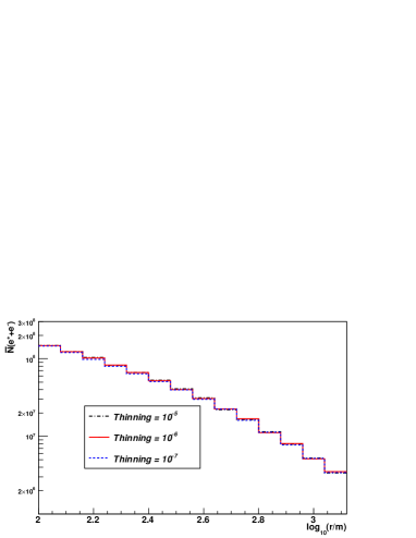
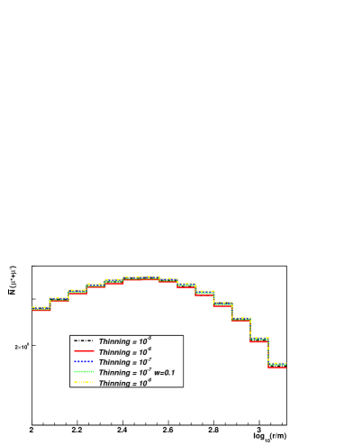
Figure 4: Average number $\bar{N}$ of electrons (left panel) and muons (right panel) at ground as a function of the logarithm of the distance to the core. 100 proton-showers of energy $10^{19}$ eV and $\theta=0^{\circ}$ were simulated with different thinning levels as indicated in the insets.

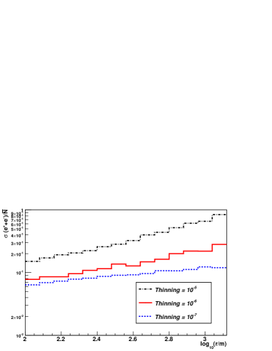
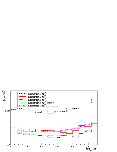
Figure 5: The relative fluctuation $\sigma/\bar{N}$ in the number of electrons (left panel) and muons (right panel) at ground, as a function of the logarithm of the distance to the shower core, for the same sets of shower simulations as in Fig. 4.

Firstly in Fig. 4 we show the average number $\bar{N}$ of electrons (left panel) and muons (right panel) versus the distance to the shower axis $r$ for different thinning levels. As can be seen, the result is rather independent of the thinning level. This is not the case for the relative fluctuations $\sigma/{\bar{N}}$ shown in Fig. 5, which depend strongly on the thinning level used in the simulations. For both electron and muons $\sigma/\bar{N}$ has a minimum at the distance at which the number of particles is largest. Also, as expected, the fluctuations can be seen to converge to a common value at each distance as the thinning level decreases, because the effect of thinning is increasingly less important. The artificial fluctuations introduced by thinning in the case of electrons, do not contribute equally to the total fluctuation at all distances from the core as expected. It can be seen for instance that the relative fluctuation rises with $r$ but the increase is smaller the smaller the thinning level.

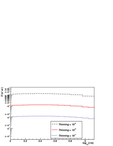
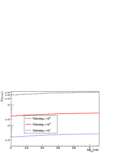
Figure 6: Average weight $\bar{w}$ of the distribution of weights of electrons (left panel) and muons (right panel) at ground, as a function of the logarithm of the distance to the shower core, for sets of 100 proton-induced showers at $10^{19}$ eV and $\theta=0^{\circ}$, simulated with different thinning levels as indicated in the insets.

In Fig. 6 we plot the average weight $\bar{w}$ assigned in the process of thinning to electrons (left panel) and muons (right panel) as a function of the distance to the shower axis. In both cases the average weight is simply proportional to the thinning level $\bar{w}\propto R_{\rm thin}$, as expected. The average weight of electrons is typically 50 times larger than that of the muons. For electrons the average weight decreases at large distances to the core, because far from the core the electrons are mainly produced by muon decay, and muons carry a smaller weight. For the muons, there is a mild increase with $r$ because the highest energy muons, which typically carry a small weight (i.e. they are less thinned than lower energy muons), are typically produced close to shower axis.

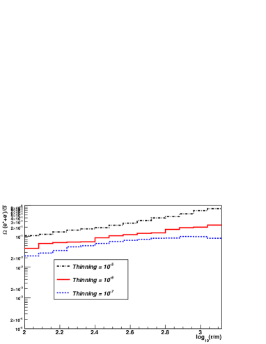
Figure 7: Relative fluctuations of the distribution of weights ($\Omega/\bar{w}$) of electrons (left panel) and muons (right panel) at ground as a function of the logarithm of the distance to the core, for the same sets of shower simulations as in Fig. 6.

In Fig. 7 we plot the relative fluctuations of the distribution of weights $\Omega/\bar{w}$, for electrons (left panel) and muons (right panel) as a function of distance to the shower core. As expected the fluctuation of the weight decreases as $R_{\rm thin}$ decreases and the showers are less thinned. Also, for values of $R_{\rm thin}<10^{-5}$ the relative fluctuation $\Omega/\bar{w}$ is roughly independent of the thinning level, and as a consequence we have that approximately $\Omega\propto R_{\rm thin}$.

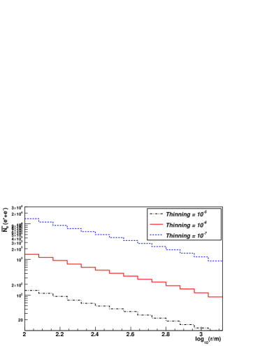
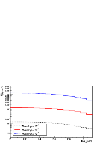
Figure 8: Average number of entries (non-thinned particles) $\bar{N}_{e}$ for electrons (left panel) and muons (right panel) at ground, as a function of the logarithm of the distance to the core, for the same sets of shower simulations as in Fig. 6.

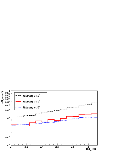
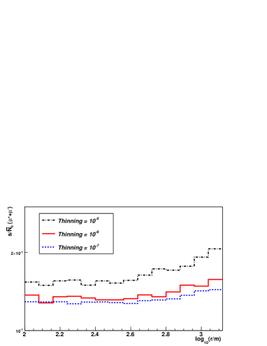
Figure 9: Relative fluctuation ($s/\bar{N}_{e}$) of the distribution of the number of entries for electrons (left panel) and muons (right panel) at ground, as a function of the logarithm of the distance to the core, for the same sets of shower simulations as in Fig. 6.

In Fig. 8, we show the average number of entries $\bar{N}_{e}$ for the same simulations as in Fig. 6 above. Clearly, we have that $\bar{N}_{e}\propto R_{\rm thin}^{-1}$ as imposed by the constraint in Eq. (4) that the average number of particles $\bar{N}$ has to be independent of $R_{\rm thin}$, together with the fact that $\bar{w}\propto R_{\rm thin}$. In Fig. 9, we show the relative fluctuation in the number of entries $s/{\bar{N}_{e}}$. For small thinning levels ($R_{\rm thin}<10^{-6}$), we find that the relative fluctuation is approximately independent of the thinning level, implying that $s\propto R_{\rm thin}^{-1}$.

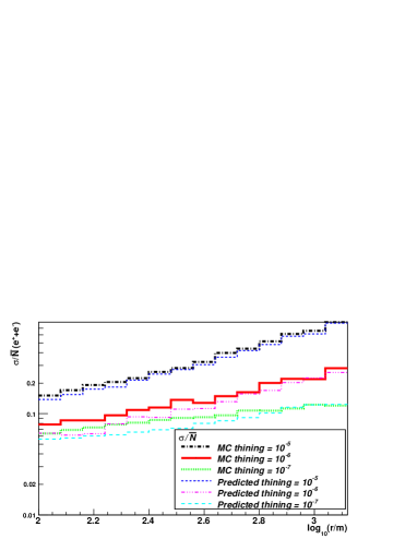
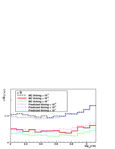
Figure 10: Relative fluctuations $\sigma/\bar{N}$ of the distribution of number of electron (left panel) and muons (right panel) at ground, as a function of the logarithm of the distance to the core, for the same sets of shower simulations as in Fig. 6. The $\sigma/\bar{N}$ obtained in the simulations (MC) is compared to that predicted by Eq. (5).

Finally, in Fig. 10, we compare the relative fluctuation of the number of particles $\sigma/\bar{N}$ obtained directly in Monte Carlo simulations, with that predicted by Eq. (5), using the values of $\bar{w}$, $\Omega$, $\bar{N}_{e}$ and $s$ obtained in the same simulations. The comparison is shown for thinning levels $R_{\rm thin}=10^{-5},\leavevmode\nobreak\ 10^{-6}$ and $10^{-7}$. The agreement between the $\sigma/\bar{N}$ obtained in Monte Carlo simulations, and that predicted by Eq. (5) is at the level of $<20\%$ for electrons and $<5\%$ for muons, confirming that Eq. (5) accounts for all the fluctuations (artificial and physical) appearing in the simulations of EAS with thinning.

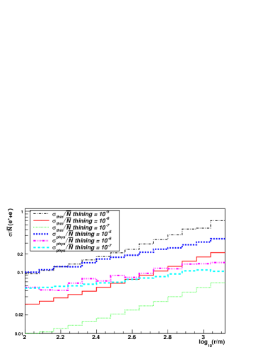
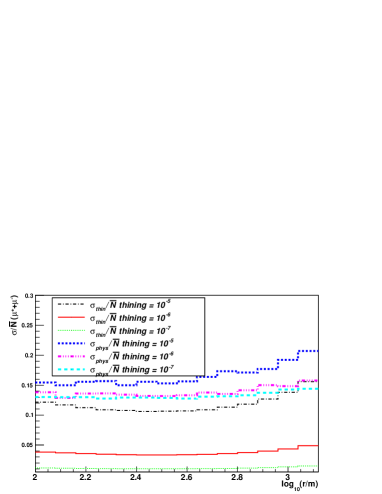
Figure 11: Relative physical $\sigma_{\rm phys}/\bar{N}$ and thinning fluctuations $\sigma_{\rm thin}/\bar{N}$ (as predicted by Eq. (5)) of the distribution of number of electron (left panel) and muons (right panel) at ground, as a function of the logarithm of the distance to the core, for the same sets of shower simulations as in Fig. 6.

From the scalings with $R_{\rm thin}$ of the different magnitudes involved in Eq. (5) obtained before, it is straightforward to deduce that $\sigma_{\rm thin}\propto R_{\rm thin}$, while $\sigma_{\rm phys}$ should be approximately independent of $R_{\rm thin}$. This is seen in Fig. 11: For thinning levels $R_{\rm thin}\sim 10^{-6}$ and smaller, $\sigma_{\rm phys}$ is almost independent of $R_{\rm thin}$, while $\sigma_{\rm thin}$ depends strongly on $R_{\rm thin}$. In Fig. 11, it can also be seen that as the thinning level decreases the $\sigma_{\rm phys}$ term increasingly dominates. This is of course expected, but it is remarkable that it was obtained from Monte Carlo simulations, and therefore it gives a strong support to our identification of $\sigma_{\rm phys}$ with the true physical fluctuations.

4.2.2 Dependence of fluctuations at ground on the number of particles

Let us now consider the dependence of the fluctuations on the size of the ring around a distance to the shower core $r$, where particles are collected in the simulation. Let us consider how the density of particles is evaluated. If $\bar{N}(r,\Delta r)$ is the average number of particles at distance $r$ in a small bin $\Delta r$ (here we assume cylindrical symmetry around the shower axis, but the argument does not depend on this simplification), then the density of particles $\rho(r)$ can be defined as

$$\rho(r)={\rm lim}_{\Delta r\rightarrow 0}\;\;\frac{\bar{N}(r,\Delta r)}{2\pi r\Delta r}.$$ (8)

In the limit $\Delta r\rightarrow 0$, $\rho(r)$ is finite, at least for $r\neq 0$. However, the same is not true for the fluctuations, so that in general one can not define a “density of fluctuations” $\rho_{\sigma}(r)$. We can see this in a simple example. Assume that $\sigma(r,\Delta r)$ is the standard deviation of the distribution of the number of particles in a bin of size $\Delta r$ and at a distance $r$. One could try to define the density of fluctuations as

$$\rho_{\sigma}(r)={\rm lim}_{\Delta r\rightarrow 0}\;\;\frac{\sigma(r,\Delta r)}{2\pi r\Delta r}.$$ (9)

If the fluctuations in the number of particles at ground were purely Poissonian, we would have

$$\sigma(r,\Delta r)=\sqrt{N(r,\Delta r)},$$ (10)

and therefore,

$$\rho_{\sigma}(r)={\rm lim}_{\Delta r\rightarrow 0}\;\;\frac{\sqrt{N(r,\Delta r)}}{2\pi r\Delta r}={\rm lim}_{\Delta r\rightarrow 0}\;\;\frac{\sqrt{2\pi r\Delta r\rho(r)}}{2\pi r\Delta r}={\rm lim}_{\Delta r\rightarrow 0}\;\;\frac{\sqrt{\rho(r)}}{\sqrt{2\pi r\Delta r}}\rightarrow\infty,$$ (11)

i.e., we can not define a density of fluctuations for Poissonian shower to shower fluctuations in the number of particles. The dependence on bin-size has been identified with the fractal structure of showers [13]. In the case of Poissonian fluctuations in the number of particles, the deduced behaviour is $\rho_{\sigma}(r)\propto\Delta r^{\alpha}$ with $\alpha=-1/2$, and we would be tempted to identify the coefficient $\alpha$ with a fractal exponent. However notice that for a Poissonian process no fractal structure is implied at all and it would be erroneous to call it a fractal exponent.

On the other hand, in the case in which the fluctuations behave as:

$$\sigma(r,\Delta r)=f(r)\Delta r+{O}(\Delta r^{2}),$$ (12)

where $f(r)$ is a function that does not depend on $\Delta r$, one can define a density of fluctuations as can be shown trivially applying Eq. (9). Remarkably, this is precisely the case of Furry’s fluctuations [14], in which $\sigma\sim N=2\pi r\rho(r)\Delta r$ and then $\rho_{\sigma}$ would be independent of $\Delta r$, i.e. $\alpha=0$. Recall that Furry statistics appears as a extremely simplified model of shower fluctuations [14], but it does take into account the branching structure of the shower (and therefore has an implicit fractal structure included).

To our knowledge, the actual behaviour of the fluctuations of showers and its dependence with the bin size is an open theoretical problem, with the theoretical prejudice ranging between two extremes: purely Poissonian fluctuations $\sigma\sim{\sqrt{N}}$, and stronger fluctuations $\sigma\sim N$. For instance, for the longitudinal development of showers one can show that in fact both types of behaviour occur [15], i.e.,

$$\sigma^{2}=a\,N^{2}+b\,N,$$ (13)

where $a$ and $b$ vary slowly with primary energy [15]. Near the maximum of the shower, the first term dominates and fluctuations are not Poissonian. For the lateral distribution no such result exists but one would expect a similar conclusion.

In Fig. 12, we show the relative fluctuation in the number of particles $\sigma/\bar{N}$, as a function of the bin size $\Delta r$, for several zenith angles $\theta$ and distances $r$ to the shower axis. Note that $\sigma/\bar{N}$ is equal to $\rho_{\sigma}$ in the limit of $\Delta r\rightarrow 0$. A fit to a power law dependence (as suggested by the discussion above) gives $\sigma/\bar{N}\propto\Delta r^{\alpha}$ with $\alpha=-1/2$ for both electrons and muons. As explained above this is suggestive of the fluctuations being Poissonian. However, if we split the fluctuations with the aid of Eq. (5) into thinning fluctuations, and physical fluctuations, it can be seen in Fig. 13 that $\sigma_{\rm phys}/\bar{N}$ is consistent with being flat with $\Delta r$, whereas $\sigma_{\rm thin}/\bar{N}$ behaves as a power law (a fit gives $\sigma_{\rm thin}/\bar{N}\propto\Delta r^{-1/2}$). These results suggest that the artificial fluctuations are Poissonian, while physical fluctuations behave as $\sigma_{\rm phys}\propto N$.

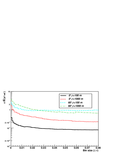
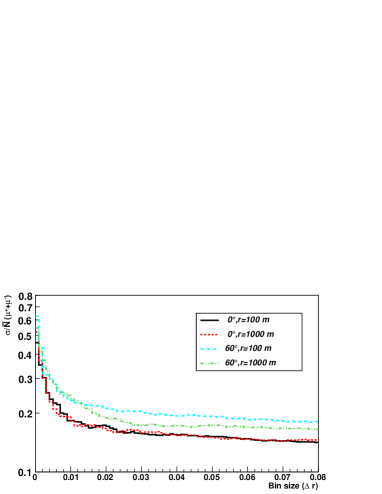
Figure 12: Relative fluctuations $\sigma/\bar{N}$ of the distribution of the number of electrons (left panel) and muons (right panel) in a ring of width $\Delta r$, centered at different $r$ at ground, as a function of the logarithm of the size of the bin $\Delta r$. 100 proton-induced showers of $10^{19}$ eV energy were simulated at different $\theta$ and fixed thinning level $R_{\rm thin}=10^{-6}$

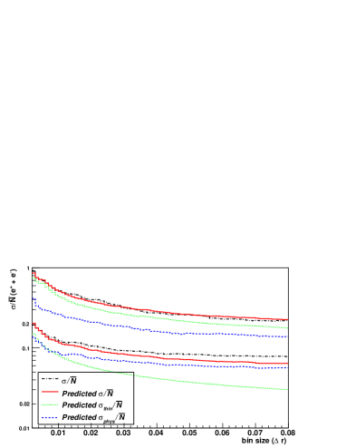
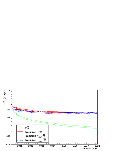
Figure 13: Relative fluctuations $\sigma/\bar{N}$ of the distribution of the number of electrons (left panel) and muons (right panel) in a ring of width $\Delta r$, centered at different $r$ at ground, as a function of the logarithm of size of the bin $\Delta r$. The upper lines correspond to simulations performed with relative thinning level $R_{\rm thin}=10^{-5}$ and the lower lines are for $R_{\rm thin}=10^{-7}$. The $\sigma/\bar{N}$ obtained in the simulations is compared to that predicted by Eq. (5). The two terms in Eq. (5) corresponding to fluctuations induced by thinning $\sigma_{\rm thin}$ and physical fluctutations $\sigma_{\rm phys}$ are also shown, see insets.

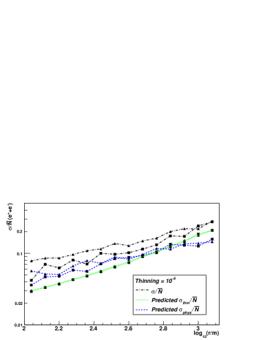
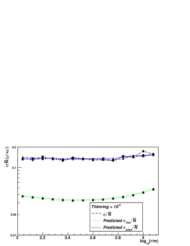
Figure 14: Relative fluctuations $\sigma/\bar{N}$ of the distribution of number of electron (left panel) and muons (right panel) at ground, as a function of the logarithm of the distance to the core, for $10^{19}$ eV proton showers with $\theta=0^{\circ}$, and relative thinning level $R_{\rm thin}=10^{-6}$. We show (squares) the result of fixing the first interaction depth at 44.9 g/cm² (mean interaction depth of $10^{19}$ eV proton-air collisions predicted by the QGSJET01 model), and also the case in which the depth of first interaction fluctuates (triangles). The $\sigma/\bar{N}$ obtained in the simulations is compared to that predicted by Eq. (5). The two terms in Eq. (5) corresponding to fluctuations induced by thinning $\sigma_{\rm thin}$ and physical fluctutations $\sigma_{\rm phys}$ are also shown in all cases, see insets.

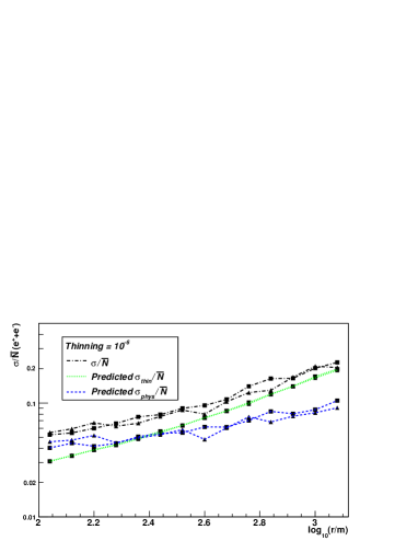
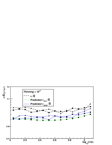
Figure 15: Same as Fig. 14 for iron-induced showers. In the simulations with fixed first interaction depth, that depth was chosen at 10.7 g/cm² (corresponding to the mean interaction depth of $10^{19}$ eV iron-air collisions predicted by the QGSJET01 model). Same symbols and line types as in Fig. 14.

5 Dependence of shower to shower fluctuations on composition and depth of first interaction

In this Section we study the influence of the fluctuations in the depth of first interaction on the overall shower to shower fluctuations of the number of particles. In Figs. 14 and 15 we plot the relative fluctuations $\sigma/\bar{N}$ in $10^{19}$ eV proton and iron-induced showers respectively. In all panels we show the results of our regular simulations, together with the results of a special set of simulations performed by fixing the depth of first interaction of the primary particle (proton or iron) at the value of its mean interaction depth predicted by the QGSJET model (namely 44.9 g/cm² for proton at $10^{19}$ eV and 10.7 g/cm² for iron at the same energy). In all cases we use Eq. (5) to split the fluctuations into artificial and physical fluctuations, and we also show them in the figures.

Firstly, it is interesting to see that the artificial fluctuations in the number of electrons or muons in iron showers are approximately equal to those in proton showers, while the physical fluctuations are smaller in iron than in proton-induced showers. The latter observation is a well-known effect which is attributed to the fact that showers initiated by a nuclei can be considered, in a first approximation, as a superposition of $A$ (atomic mass) nucleons, each with an energy $E/A$ with $E$ the energy of the primary nucleus.

It is rather remarkable that the relative fluctuations in the number of particles $\sigma/\bar{N}$ in the two different sets of simulations (fixing or varying the depth of the first interaction point), are essentially the same. This conclusion applies to both the number of electrons and the number of muons. One could think that this is due to the fluctuations induced by thinning which mask the effect of the fluctuations of the depth of first interaction, however this does not seem to be the case, since as can be seen in Figs. 14 and 15, neither the first term of Eq. (5) (the thinning fluctuations), nor the second term (the physical fluctuations) change much when varying or fixing the depth of first interaction. We conclude that the relative shower to shower fluctuations on the number of particles at ground $\sigma/\bar{N}$ are rather insensitive to the physical fluctuations of the depth of first interaction. This is related to the fact that the maximum of a shower at $\theta=0^{\circ}$, where the fluctuations are minimum [11], occurs near the ground. For other zenith angles a small difference appears in the physical fluctuations of the simulations performed with fixed and fluctuated first interaction point.

6 Conclusions

In this work we have performed a comprehensive study of shower to shower fluctuations by means of Monte Carlo simulations of extensive air showers. An understanding of the shower to shower fluctuations will help to improve the interpretation of cosmic-ray data.

We have shown that the determination of the true, physical shower to shower fluctuations is hampered by the thinning procedure necessary to simulate in a practical manner air showers at EeV energies and above. However, we also show that the artificial fluctuations induced by thinning ($\sigma_{\rm thin}$) can be identified and splitted from the physical fluctuations ($\sigma_{\rm phys}$) with the aid of Eq. (5), which we have shown to account for all, true and artificial fluctuations appearing in the simulations. Eq. (5) reproduces the expectation that as the thinning level decreases $R_{\rm thin}\rightarrow 0$, and showers are less thinned, then the artificial fluctuations decrease, the physical ones become dominant, and they do not depend on $R_{\rm thin}$.

Our simulations also indicate that the physical shower to shower fluctuations of the number of particles at ground behave proportionally to the number of particles $N$, while the artificial fluctuations are Poissonian, i.e., behave as $\sqrt{N}$.

Besides, we have shown that the size of the relative fluctuations due to the depth at which the first interaction initiating the shower occurs, is smaller or of the same order as the fluctuations occuring in the subsequent secondary interactions in the shower.

7 Appendix

In this Appendix, we calculate the probability distribution of the number of particles $N$ in a given bin of $r$ distance to shower core, or of energy. making some simplifying assumptions. We want to calculate the probability distribution of particles, possibly in a given bin of $r$ or of energy. We will assume that the probability for an entry (a non-thinned particle) to have a weight $w_{i}$ is given by $P_{w}(w_{i})$. In addition the number of entries, $N_{e}$ in a given shower is a random variable with probability distribution $P_{e}(N_{e})$. Our main simplifying assumption is the following: we will assume that $P_{w}$ and $P_{e}$ are independent of each other. This assumption is only approximate, because in a shower simulated with thinning both the entries and the weight assigned to each particle are controlled by the branching of the shower and therefore they must be related. However, as we will see a posteriori, the approximation is good enough for our purposes here, and it serves to clarify the role of thinning.

Under this approximation we can write the probability $P(N)$ of having $N$ particles as,

$$P(N)=\sum_{N_{e}}P_{e}(N_{e})\left[\int dw_{1}\cdots dw_{N_{e}}\;P_{w}(w_{1})\cdots P_{w}(w_{N_{e}})\;\delta(w_{1}+\cdots+w_{N_{e}}-N)\,\right].$$ (14)

where the $\delta-$function expresses the constraint that the sum of weights is equal to the total number of particles.

In what follows we evaluate this expression first by making further assumptions about the shape of $P_{e}$ and $P_{w}$, and afterwards in the general case using the characteristic function, related to the probability distribution. The definitions of cumulants and of the characteristic function can be found in any text book on statistics, for instance [16].

We start with the integral

$$I(N_{e},N)=\int dw_{1}\cdots dw_{N_{e}}\;P_{w}(w_{1})\cdots P_{w}(w_{N_{e}})\;\delta(w_{1}+\cdots+w_{N_{e}}-N),$$ (15)

and introduce the Fourier representation for the delta function.

$$I(N_{e},N)=\int dw_{1}\cdots dw_{N_{e}}\;P_{w}(w_{1})\cdots P_{w}(w_{N_{e}})\;\;\frac{1}{2\pi}\int dk\;e^{ik(w_{1}+\cdots+w_{N_{e}}-N)}.$$ (16)

Changing the order of integration gives

$$I(N_{e},N)=\frac{1}{2\pi}\int dk\leavevmode\nobreak\ e^{-ik\,N}\int dw_{1}\;P_{w}(w_{1})e^{ik\,w_{1}}\cdots\int dw_{N_{e}}\;P_{w}(w_{N_{e}})e^{ik\,w_{N_{e}}}$$

$$=\frac{1}{2\pi}\int dke^{-ik\,N}\left[\int dwP_{w}(w)e^{ikw}\right]^{N_{e}}.$$ (17)

To further continue with the evaluation of $P(N)$ we need to make additional approximations. We assume that $P_{w}$ is a Gaussian distribution with average $\bar{w}$ and rms $\Omega$

$$P_{w}(w)=A\;e^{-(w-\bar{w})^{2}/(2\Omega^{2})},$$ (18)

where $A=1/\sqrt{2\pi\Omega^{2}}$ is the probability normalization. Its Fourier transformation is given by

$$\int dw\;e^{ikw}\;\;P_{w}(w)=e^{ik\bar{w}}\;e^{-k^{2}\Omega^{2}/2}.$$ (19)

Therefore,

$$I(N_{e},N)=\frac{1}{2\pi}\int dk\;e^{-ik(N-N_{e}\bar{w})}\;\;e^{-N_{e}k^{2}\Omega^{2}/2},$$ (20)

For large values of $\bar{N}_{e}$, the sum in Eq. (14) can be approximated by an integral

$$P(N)=\sum_{N_{e}}\,P_{e}(N_{e})\;I(N_{e},N)\;\approx\int dN_{e}\;P(N_{e})\;I(N_{e},N).$$ (21)

If we assume that $P_{e}(N_{e})$ is also a Gaussian with average $\bar{N}_{e}$ and standard deviation $s$ and inserting Eq. (20) in Eq. (21) gives

$$P(N)=\frac{1}{2\pi}\int dk\;e^{-ikN}\int dN_{e}\;\frac{1}{\sqrt{2\pi s^{2}}}\;e^{-(N_{e}-\bar{N}_{e})^{2}/(2s^{2})}\;e^{ikN_{e}\bar{w}}\;e^{-k^{2}N_{e}\Omega^{2}/2}.$$ (22)

The integral over $N_{e}$ can be done analytically

$$P(N)=\frac{1}{2\pi}\int dk\;e^{-ikN}\;\;\exp[\,i\bar{N}_{e}\bar{w}k-\frac{1}{2}(\bar{N}_{e}\Omega^{2}+s^{2}\bar{w}^{2})k^{2}+{O}(k^{3})\,].$$ (23)

where we neglect in the exponential powers of $k$ larger than 2, after applying the saddle point approximation. We arrive at the final expression

$$P(N)=\frac{1}{\sqrt{2\pi\sigma^{2}}}e^{-(N-\bar{N})^{2}/(2\sigma^{2})},$$ (24)

where

$$\bar{N} =\bar{N}_{e}\bar{w},$$

$$\sigma^{2} =\bar{N}_{e}\Omega^{2}+\bar{w}^{2}s^{2}.$$ (25)

Notice that the above expressions have the correct asymptotic behaviour. If the particles have no weight, $\bar{w}\rightarrow 1$ and $\Omega\rightarrow 0$, then the average number of particles is equal to the average number of entries (non-thinned particles) $\bar{N}=\bar{N}_{e}$ and $\sigma=s$. On the extreme case of a strongly thinned shower in which all particles are grouped together in a single entry ($\bar{N}_{e}=1,s=0$) then $\bar{N}=\bar{w}$ and $\sigma=\Omega$, as expected.

The above result is general and valid for any probability distribution for $P_{w}$ and $P_{e}$. The only requirement is the “factorization” property given in Eq. (14). From Eq. (17), we introduce the characteristic function for the probability distribution $P_{w}$,

$$\tilde{P}_{w}(k)=\int dw\;P_{w}(w)\;e^{ikw},$$ (26)

which, in general can be written as

$$\tilde{P}_{w}(k)=\exp[\;ika_{1}-\frac{1}{2}a_{2}k^{2}+\cdots]=e^{ig(k)},$$ (27)

where the coefficients of the expansion of $g(k)$ are related to the cumulants of the distribution of $P_{w}$. For instance $a_{1}=\bar{w}$, $a_{2}=\Omega^{2}$, etc. Then Eq. (14) reads

$$P(N)=\frac{1}{2\pi}\int dk\;e^{-ikN}\int dN_{e}\;P_{e}(N_{e})\;e^{iN_{e}g(k)}.$$ (28)

We define

$$\tilde{P}_{e}(q)=\int dN_{e}\;P_{e}(N_{e})\;e^{iqN_{e}}=\exp[\;ib_{1}q-\frac{1}{2}b_{2}q^{2}+\cdots],$$ (29)

where as before $b_{1}=\bar{N}_{e}$ and $b_{2}=s^{2}$. Then we get

$$P(N)= \frac{1}{2\pi}\int dk\;e^{-ikN}\;\tilde{P}_{e}(g(k))$$

$$= \frac{1}{2\pi}\int dk\;e^{-ikN}\;\exp[\;ib_{1}g(k)-\frac{1}{2}b_{2}g(k)^{2}+\cdots].$$

Where the function $g(k)=k\bar{w}+i/2\;k^{2}\Omega^{2}+\cdots$. Then after some algebra

$$P(N)=\frac{1}{2\pi}\int dk\;e^{-ikN}\;\exp[\;ik\bar{w}\bar{N}_{e}-\frac{1}{2}k^{2}(s^{2}\bar{w}^{2}+\bar{N}_{e}\Omega^{2})+\cdots\;]$$ (30)

The coefficients of the expansion around $k=0$ are again the cumulants of the distribution $P(N)$, therefore we simply read the result given above in Eq. 25. But, as a bonus, we obtain also all the other cumulants. For instance for the skewness we obtain

$$\gamma_{3}=\frac{M_{3}}{\sigma^{3}}=\frac{1}{\sigma^{3}}\times(m_{3}\bar{N}_{e}+3\bar{w}s^{2}\Omega^{2}+\bar{w}^{3}M_{e}),$$ (31)

where $m_{3}$ is the third central moment ( $m_{3}=\langle(w-\bar{w})^{3})\rangle\;$) of the weight distribution and $M_{e}$ is the third central moment of the distribution of the number of entries. In the same way, one can easily obtain other cumulants from the above expressions.

8 Acknowledgements

We thank V. Canoa, G. Rodriguez–Fernandez, T. Tarutina, I. Valiño and E. Zas for discussions and comments. P. M. H. was supported by Juan de la Cierva grant. We thank Centro de Supercomputación de Galicia (CESGA) for computer resources. This work was made possible with support from the Ministerio de Ciencia e Innovación, Spain under grant FPA 2007-65114 and Consolider CPAN; and of ALFA-EC funds in the framework of the HELEN (High Energy Physics Latin-American-European Network) project. J. A-M also thanks Xunta de Galicia (INCITE09 206 336 PR) for financial support.

References

- [1] M. Nagano, A. Watson, Rev. Mod. Phys. 72, 689 (2000), and references therein.
- [2] C.A. García Canal et al. Phys. Rev. D 79, 054006 (2009), and refs. therein.
- [3] A. M. Hillas, Proc of the Paris Workshop on Cascade simulations, J. Linsley and A. M. Hillas (eds.), p. 39 (1981); A.M. Hillas, Nucl. Phys. B (Proc. Suppl.) 52B, 29 (1997).
- [4] S. J. Sciutto, Proc. 27th ICRC (Hamburg) 1 237 (2001).
- [5] S. J. Sciutto, AIRES User’s Manual and Reference Guide; version 2.6.0 (2002), available electronically at www.fisica.unlp.edu.ar/auger/aires.
- [6] N. N. Kalmykov and S. S. Ostapchenko, Yad. Fiz. 56, 105 (1993); Phys. At. Nucl. 56, 346 (1993); N. N. Kalmykov, S. S. Ostapchenko, and A. I. Pavlov, Bull. Russ. Acad. Sci. (Physics) 58, 1966 (1994).
- [7] M. Kobal et al., Pierre Auger collaboration, Astropart. Phys. 15, 259 (2001).
- [8] F. Schmidt, M. Ave, L. Cazon, and A. S. Chou, Astropart. Phys. 29, 355 (2008).
- [9] P. Billoir, Astropart. Phys. 30, 270 (2008).
- [10] M. Ave, et al. Nucl. Instrs. and Meths. in Phys. Res. A 578, 180 (2007).
- [11] T.K. Gaisser, Cosmic Rays and Particle Physics, Cambridge Univ. Press (1992).
- [12] M. Risse, et al., Proc. of 27th ICRC 2001, p. 522. Hamburg, Germany.
- [13] J. Kempa and M. Samorski, J. Phys. G: Nucl. Part. Phys. 24, 1039 (1998).
- [14] W.H. Furry, Phys. Rev. 52, 569 (1937).
- [15] R.A. Vazquez, Astropart. Phys. 6, 411 (1997).
- [16] See for instance, W.T. Eadie et al., Statistical Methods in experimental physics, North-Holland Pub., Amsterdam (1971).