Andreev transport in two-dimensional normal–superconducting systems in strong magnetic fields

Abstract

The conductance in two–dimensional (2D) normal–superconducting (NS) systems is analyzed in the limit of strong magnetic fields when the transport is mediated by the electron–hole states bound to the sample edges and NS interface, i.e., in the Integer Quantum Hall Effect regime. The Andreev–type process of the conversion of the quasiparticle current into the superflow is shown to be strongly affected by the mixing of the edge states localized at the NS and insulating boundaries. The magnetoconductance in 2D NS structures is calculated for both quadratic and Dirac–like normal state spectra. Assuming a random scattering of the edge modes we analyze both the average value and fluctuations of conductance for an arbitrary number of conducting channels.

1 Introduction

Andreev transport phenomena, i.e., transport effects associated with the conversion of electrons into holes, are known to determine the distinctive features of a wide class of hybrid structures consisting of the normal (N) and superconducting (S) metal parts (see, e.g., [1] and references therein). Applying rather high magnetic fields one can drastically affect the physics of these Andreev–type effects due to a strong modification of the transport mode structure [2, 3, 4, 5] which is typical for the systems in the Integer Quantum Hall Effect (IQHE) regime. Provided the radii of the cyclotron orbits in the normal part of the system become less than the mean free path the transport appears to be determined by the waves bound to the sample edges. Depending on the momenta of these waves and quasiparticle charge the transport modes are localized near the different edges and, thus, the wavefunctions of the incoming and outgoing particles appear to be spatially separated. Thus, the magnetic field destroys the basic backscattering property of the standard Andreev reflection.

It is the goal of the present work to suggest a general theoretical description of the Andreev transport mediated by the edge states in the IQHE regime. We consider here an exemplary two–dimensional (2D) NS system shown in Fig. 1. Such type of mesoscopic junctions based on a 2D electronic gas (2DEG) or gapless 2D semiconductors like graphene are in the focus of current experimental and theoretical research [2, 3, 4, 5, 6, 7, 8, 9, 10]. To elucidate our main results we start here from a qualitative description of the transport mediated by the edge states. An electron injected from the normal conductor goes to the superconductor through an edge state “a”. At the “ab”-corner it transforms into two types of hybridized electron-hole states at the boundary ”b” with the probabilities $\tau_{1}$ and $(1-\tau_{1})$, respectively (see the inset of Fig. 1). Similarly to the situation at the “ab”-corner each of electron-hole quasiparticles transforms with the probabilities $\tau_{2}$ and $(1-\tau_{2})$ into an electron and a hole which return to the normal lead through the edge states ”c”. Without mode mixing ($\tau_{1,2}=0$ or $1$) each initial electron (hole) state at the boundary ”a” completely transforms into the final electron (hole) state at the boundary ”c” and the probability of the electron–hole conversion is zero, so that the total conductance $G$ vanishes.

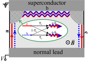
Figure 1: (Color online) The junction between the superconductor and the chiral metal [edge states in high mobility 2D metal in the IQHE regime]. Solid (dotted) lines correspond to the electron (hole) edge states at “a” and “c” insulating boundaries, and wavy lines correspond to the hybridized electron-hole modes at the superconducting boundary “b”. Inset: Edge mode scattering from insulating edge “a” to superconducting edge “b” with probabilities $\tau_{1}$ and $(1-\tau_{1})$.

Taking account of the quasiparticle mode mixing at the corners we find:

$$G=2G_{0}N\left[\tau_{1}(1-\tau_{2})+\tau_{2}(1-\tau_{1})\right]\ ,$$ (1)

where $G_{0}=e^{2}/\pi\hbar$ is the conductance quantum, and $N$ is the number of propagating electron edge states. Thus, it is the mode mixing which is responsible for the conversion of the quasiparticle current into the supercurrent outgoing from the NS boundary.

Generally, the solution of the problem of coupling between the edge states near the corner is rather complicated and depends on the details of the system geometry. Therefore only limiting cases have been previously considered: (i) quasiclassical limit with the large number of the edge states, when the problem can be treated considering the particles and holes on the cyclotron orbits skipping along the surface [3]; (ii) quantum limit when the number of the edge states is of the order of unity [4, 5]. The first case corresponds to rather large Fermi energies comparing to the Landau level spacing. The corresponding oscillating behavior of the conductance of the 2D NS junction vs magnetic field, junction width and/or Fermi level has been analyzed in detail in Refs. [3, 2].

In this Letter we analyze the magnetoconductance behavior in the NS structures for an arbitrary number of transport modes taking into account the mixing of the edge states near the corners. Adopting a phenomenological description of the mode mixing problem based on the transfer matrix approach we find a simple expression for the conductance in the quantum limit. Such model suggests a simple explanation of the oscillatory phenomena mentioned above and brings out their dependence on the mode coupling parameters. To find the conductance for an arbitrary number of quantum channels we assume the mode mixing at the corners to be random in the sense that the appropriate scattering matrices are uniformly distributed (see below for details). Such approach allows us to find universal expressions for the average conductance and its fluctuations which depend only on fundamental constants and number of transport channels:

$$\langle G\rangle=G_{0}N\ ,$$ (2)

$$\sigma_{G}=\sqrt{\left<G^{2}\right>-\left<G\right>^{2}}=G_{0}\sqrt{\frac{N}{4(2N+1)}}\ .$$ (3)

In the equation (2) contribution of each electron transport mode to the conductance equals to the conductance quantum $G_{0}$ instead of $2G_{0}$ in ballistic NS-junctions without magnetic field. Such conductance reduction is caused by the levelling of outgoing (along the “c”-edge) electron and hole probabilities in the limit of strong disorder, which saturate at the value 1/2. Such levelling is analogous to the one observed in numerical simulations in [5] for the tight-binding model with the disorder in on-site energies.

2 Basic equations and edge state spectra

The spectra of quasiparticle edge states can be found using the Bogolubov–de Gennes (BdG) equations written for electron–like ($u$) and hole–like ($v$) parts of the wave function $\hat{\Psi}=(\hat{u},\hat{v})$:

$$\left(\begin{array}[]{cc}\hat{H}-\mu&\Delta\\ \Delta^{*}&\mu-\mathcal{T}\hat{H}\mathcal{T}^{-1}\end{array}\right)\hat{\Psi}=E\hat{\Psi}\ .$$ (4)

Here $\mathcal{T}$ is the time–reversal operator, $\Delta$ is the gap operator, and the energy $E$ is measured relative to the Fermi level $\mu$. Note that we neglect here the Zeeman shift of the quasiparticle spectra caused by the interaction of magnetic field with the true electron spin.

For 2DEG the single particle hamiltonian $\hat{H}$ takes the Schrödinger form $\hat{H}({\bf A})=({\bf p}-\frac{e}{c}{\bf A})^{2}/2m$, where ${\bf p}=-i\hbar({\partial}/{\partial x};\partial/\partial y)$ is the momentum operator in the x-y plane of the 2D system, and ${\bf A}$ is the vector potential corresponding to the magnetic field ${\bf B}$ perpendicular to the system plane. In graphene there appear 2 sublattice (pseudospin) and 2 valley (isospin) degrees of freedom and in the ”valley-isotropic” basis the hamiltonian could be written as follows: $\hat{H}=v_{F}\tau_{0}\otimes\sigma\left({\bf p}-\frac{e}{c}{\bf A}\right)$ (see, e.g., [4]). Here $v_{F}$ is the Fermi velocity, $\sigma_{i}$ and $\tau_{i}$ are the Pauli matrices acting in the sublattice and valley spaces, respectively, and $\sigma_{0}$, $\tau_{0}$ are the $2\times 2$ unit matrices.

The boundary conditions and corresponding edge state spectra at the boundaries with isolator and superconductor have been previously studied for 2DEG [2] as well as for graphene [4, 11, 12, 13]. The boundary condition at the NS interface with 2DEG couples electron $u$ and hole $v$ parts of wave function and in quasiclassical limit takes the usual form $v=e^{-i\beta}u$, where $\beta=\arccos(\varepsilon/\Delta)$. The wave function at the 2DEG insulating edge vanishes $\Psi=0$. According to Akhmerov and Beenakker [4] the graphene-isolator boundary conditions

$$\Psi=\left({\bf\nu},{\bf\hat{\tau}}\right)\otimes\left({\bf n_{\bot}},{\bf\hat{\sigma}}\right)\Psi$$ (5)

are crucially determined by the isospin vector ${\bf\nu}$ while the resulting quasiparticle spectrum depends on the vector $\bf n_{\bot}$. Here the unit vector $\bf n_{\bot}$ should have a zero projection on the direction normal to the graphene edge. The graphene-superconductor (GS) interface boundary condition doesn’t depend on valley degree of freedom and for subgap energies it could be written as follows: $\hat{v}=e^{-i\beta({\bf n\cdot\sigma})}\hat{u}$. Thus, the edge state spectrum is valley degenerate.

Taking the case of a homogeneous boundary and choosing the gauge with the vector potential parallel to the boundary one can find a set of spectral branches $E_{n}(k_{\parallel})$ vs the conserved momentum component $k_{\parallel}$ along the interface. Here we introduce an integer index $n$ enumerating the branches. Thus, each insulating edge (“a” or “c”) supports $2N$ propagating edge modes: $N$ electron-like modes and $N$ hole-like modes. The NS interface also supports $2N$ propagating (valley degenerated in graphene case) modes with mixed electron-hole wave functions.

3 Mixing of the edge modes. Transfer matrix approach

Considering the transport mediated by the edge states we use a simple phenomenological model based on the transfer matrix approach. We introduce a transfer matrix $\hat{S}$ which couples the quasiparticle edge waves propagating along the “a” and “c” boundaries. This matrix calculated for the states at the Fermi level is known to determine the linear transport characteristics at zero temperature [1, 14]. It is important to note here that at the Fermi level the matrix $\hat{S}$ appears to be simultaneously a scattering matrix coupling the incoming and outgoing electron–hole waves. Indeed, in this case all the states propagating along the interfaces in Fig. 1 have the same sign of the group velocity $\partial E_{n}/\partial k_{\parallel}$ [2, 4] and, thus, all quasiparticle fluxes are flowing clockwise for a chosen magnetic field direction.

The BdG equations (4) are known to be invariant with respect to the transformation converting electrons into holes and changing the sign of energy $E$ and, as a consequence, all the edge modes can be divided into two groups connected by this transformation. For the NS interfaces we denote these groups as $g_{+}$ and $g_{-}$ while for the boundaries with an insulator (“a” and “c”) these groups just coincide with pure electron ($u_{a}$ and $u_{c}$) and hole ($v_{a}$ and $v_{c}$) waves. Each of hybrid states $g_{\pm}$ propagating along the ballistic NS boundary “b” of the length $L$ acquires a phase factor $e^{\pm ik_{n}L}$, where $k_{n}$ is the momentum satisfying the equation $E_{n}(k_{n})=0$ for the spectral branches at the NS boundary. The scattering processes at the corners “ab” and “bc” (see Fig. 1) could be described by unitary transfer matrices $\hat{T}_{1,2}$, which couple the incident and transmitted quasiparticle waves:

$$\left(g_{+}\atop g_{-}\right)=\hat{T}_{1}\left(u_{a}\atop v_{a}\right)\ ,\quad\left(u_{c}\atop v_{c}\right)=\hat{T}_{2}\left(g_{+}\atop g_{-}\right)\ ,$$ (6)

where $u_{a}$, $v_{a}$, $u_{c}$, $v_{c}$, $g_{+}$, $g_{-}$ are the sets of wave amplitudes corresponding to the solutions of BdG equations at the Fermi level. The unitarity of the matrices $\hat{T}_{1,2}$ is a consequence of the quasiparticle current conservation. The scattering matrices $\hat{T}_{1,2}$ can be conveniently presented in the four–block form:

$$\hat{T}_{1}=\left(\begin{array}[]{cc}\hat{t}_{+e}&\hat{t}_{+h}\\ \hat{t}_{-e}&\hat{t}_{-h}\end{array}\right)\ ,\quad\hat{T}_{2}=\left(\begin{array}[]{cc}\hat{t}_{e+}&\hat{t}_{e-}\\ \hat{t}_{h+}&\hat{t}_{h-}\end{array}\right)\ .$$ (7)

The total transfer matrix $\hat{S}$ can be written as a product of three matrices describing subsequent scattering and propagation processes discussed above:

$$\hat{S}=\left(\begin{array}[]{cc}\hat{s}_{ee}&\hat{s}_{eh}\\ \hat{s}_{he}&\hat{s}_{hh}\end{array}\right)=\hat{T}_{2}\hat{\Lambda}_{L}\hat{T}_{1}\ ,$$ (8)

where $\hat{\Lambda}={\rm diag}\left(e^{ik_{1}L},\ldots,e^{ik_{N}L},e^{-ik_{1}L},\ldots,e^{-ik_{N}L}\right)$ is a diagonal transfer matrix of phase factors acquired at the NS boundary. The blocks $\hat{s}_{ee},\hat{s}_{eh},\hat{s}_{he},\hat{s}_{hh}$ of the matrix $\hat{S}$ describe the scattering between the edge states at the “a” and “c” boundaries. The zero–temperature conductance is given by following expression [14]:

$$G=G_{0}{\rm Sp}\left(\hat{I}-\hat{s}_{ee}^{+}\hat{s}_{ee}+\hat{s}_{eh}^{+}\hat{s}_{eh}\right)=2G_{0}{\rm Sp}\left(\hat{s}_{eh}^{+}\hat{s}_{eh}\right)\ .$$ (9)

4 Magnetoconductance in NS junctions. Quantum limit

At sufficiently small Fermi energy $\mu$ each edge supports only two propagating modes and each block of scattering matrices becomes a single complex amplitude. It is convenient to parametrize these amplitudes as follows

$$t_{+e}=\sqrt{1-\tau_{1}}e^{i(\varphi_{1}+\theta_{1}/2)}\ ,\,t_{-e}=\sqrt{\tau_{1}}e^{i(\varphi_{1}-\theta_{1}/2)}\ ,$$ (10)

$$t_{e+}=\sqrt{1-\tau_{2}}e^{i(\varphi_{2}+\theta_{2}/2)}\ ,\,t_{e-}=\sqrt{\tau_{2}}e^{i(\varphi_{2}-\theta_{2}/2)}\ ,$$ (11)

$t_{\mp h}=\pm t_{\pm e}^{*}$, $t_{h\mp}=\pm t_{e\pm}^{*}$, where $\tau_{1}$ is the probability that electron at the boundary “a” scatters into the second type of hybrid modes, $\tau_{2}$ is the probability that the first type hybrid mode scatters into the hole at the boundary “c”. The matrix of phase factors takes the form: $\hat{\Lambda}={\rm diag}\left(e^{ik_{1}L},e^{-ik_{1}L}\right)$, where $k_{1}$ is the momentum value at which the spectral branch at the NS boundary crosses the Fermi level. Omitting the calculation details we present here the final expression for the 2DEG – superconductor junction conductance:

$$G=2G_{0}(p_{21}+p_{12}-2\sqrt{p_{12}p_{21}}\cos\gamma)\ ,$$ (12)

where $p_{nm}=\tau_{n}(1-\tau_{m})$, $\gamma=2k_{1}L+\theta_{1}+\theta_{2}$. In the symmetric geometry of Fig. 1, i.e., when the “ab” and “bc” corners have the same shape, one can expect the appearance of an additional symmetry of scattering matrices describing the mode mixing: $\hat{T}_{2}=\hat{T}_{1}^{T}$ ($p_{12}=p_{21}$). The expression for conductance in this case can be further simplified:

$$G=4G_{0}\tau(1-\tau)\left(1-\cos\gamma\right)\ ,$$ (13)

where $\tau_{1}=\tau_{2}\equiv\tau$. The conductance reveals an oscillating behavior vs the junction width $L$ which is, in fact, a consequence of quantum mechanical interference of the edge waves propagating along the NS boundary. The expression (13) is in good agreement with the qualitative arguments in the introduction: the absence of mode mixing corresponding to the limits $\tau=0$ or $\tau=1$ causes a complete suppression of the charge transport.

Considering a quantum limit for GS junctions we need to emphasize two important distinctive features. First, the momentum of the zero energy mode ($E_{1}(k_{1})=0$) at the GS boundary appears to vanish ($k_{1}=0$) and both states ($g_{+}$ and $g_{-}$) become degenerate. Second, the scattering matrices $\hat{T}_{1,2}$ crucially depend on the isospin degree of freedom. Following Ref.[4] we introduce the isospin operator eigenvectors’ basis $\left({\bf\nu}_{m},{\bf\tau}\right)\left|\pm\nu_{m}\right>=\pm\left|\pm\nu_{m}\right>$, where $\nu_{1,2}$ are the isospin vectors characterizing the “a” and “c” boundaries (see the boundary condition (5)). The scattering matrices take the form:

$$\hat{T}_{1}=\left|\nu_{1}\right>\left<\nu_{1}\right|t_{+e}+\left|-\nu_{1}\right>\left<\nu_{1}\right|t_{-e}+\\ +\left|\nu_{1}\right>\left<-\nu_{1}\right|t_{+h}+\left|-\nu_{1}\right>\left<-\nu_{1}\right|t_{-h}$$ (14)

$$\hat{T}_{2}=\left|\nu_{2}\right>\left<\nu_{2}\right|t_{e+}+\left|-\nu_{2}\right>\left<\nu_{2}\right|t_{h+}+\\ +\left|\nu_{2}\right>\left<-\nu_{2}\right|t_{e-}+\left|-\nu_{2}\right>\left<-\nu_{2}\right|t_{h-}$$ (15)

Introducing the notation $\chi=\widehat{({\bf\nu}_{1},{\bf\nu}_{2})}$ for the angle between the isospin vectors one can get the conductance of the system in the form:

$$G=2G_{0}\left[\sin^{2}\tfrac{\chi}{2}+\left(p_{21}+p_{12}\right)\cos\chi\right.\\ -2\sqrt{p_{12}p_{21}}(\cos\theta_{1}\cos\theta_{2}-\sin\theta_{1}\sin\theta_{2}\cos\chi)\\ -\sin\chi\left((1-2\tau_{1})\sqrt{p_{22}}\sin\theta_{1}\left.+(1-2\tau_{2})\sqrt{p_{11}}\sin\theta_{2}\right)\right]\ .$$ (16)

Assuming a symmetric geometry of Fig. 1 we put $\hat{T}_{2}=\hat{T}_{1}^{T}$ and find:

$$G=2G_{0}\left(2\sqrt{p}\cdot\cos\tfrac{\chi}{2}\sin\theta-(1-2\tau)\sin\tfrac{\chi}{2}\right)^{2}\ ,$$ (17)

where $\theta_{1}=\theta_{2}\equiv\theta$, $p=\tau(1-\tau)$. Contrary to the 2DEG case the conductance does not depend on the junction width $L$ which is a natural consequence of zero phase acquired by the waves propagating along the GS boundary in the two–mode limit. Another new feature specific for the case of graphene is that the additional mode mixing occurs due to the mismatch of the isospin directions at different insulating boundaries. Note that neglecting the intervalley scattering at the corners we put $\tau=0$ or $\tau=1$ and get the limit considered in Ref. [4].

5 Magnetoconductance in NS junctions. Random–matrix theory

Considering the charge transport mediated by a large number of edge states it is natural to expect that the conductance will be given by the sum of phase factors:

$$G=\sum_{ij}a_{ij}e^{i(k_{i}-k_{j})L}\ ,$$ (18)

where the hermitian matrix $a_{ij}$ is determined by the transfer matrix parameters. The oscillating behavior of conductance vs $L$ becomes more complicated than in a two–mode limit and is generally characterized by a set of incommensurable periods. Previously these oscillations have been predicted on the basis of quasiclassical method for quasiparticles moving along skipping cyclotron orbits [3]. In real experimental situation the mode interference and the corresponding oscillations should be, of course, smeared due to the effect of sample imperfections, e.g., roughness, etc. Here we suggest a phenomenological approach to treat the problem taking account of these effects for an arbitrary number of modes. We model the scattering caused by the sample imperfections introducing random transfer matrices $\hat{T}_{1,2}$ and applying standard methods for calculation of the ensemble averages [1].

The symmetry properties of the transfer matrix $\hat{T}_{m}$ allow us to introduce a polar decomposition (cf. [15, 16]): $\hat{T}_{m}=\hat{\alpha}_{m}\hat{\Theta}_{m}\hat{\beta}_{m}$, where

$$\hat{\alpha}_{m}=\left(\begin{array}[]{cc}\hat{A}_{m}&0\\ 0&\hat{A}_{m}^{*}\end{array}\right),\,\hat{\beta}_{m}=\left(\begin{array}[]{cc}\hat{B}_{m}&0\\ 0&\hat{B}_{m}^{*}\end{array}\right)\ ,$$

$$\hat{\Theta}_{m}=\left(\begin{array}[]{cc}\sqrt{1-\hat{\tau}_{m}}&\sqrt{\hat{\tau}_{m}}\\ -\sqrt{\hat{\tau}_{m}}&\sqrt{1-\hat{\tau}_{m}}\end{array}\right)\ ,$$

and the unitary matrices $\hat{A}_{m},\hat{B}_{m}$ characterize the scattering phase shifts while the diagonal matrix $\hat{\tau}_{m}={\rm diag}(\tau_{m}^{(1)},\ldots,\tau_{m}^{(N)})$ consists of the eigenvalues $\tau_{1}^{(n)}$ ($\tau_{2}^{(n)}$) of the matrix $\hat{t}_{-e}^{+}\hat{t}_{-e}$ ($\hat{t}_{e-}^{+}\hat{t}_{e-}$). The values $\tau_{m}^{(n)}$ give us the probabilities of transitions between the modes. Any scattering $2N\times 2N$-matrix $\hat{X}$ invariant under electron-hole converting transformation of BdG equations belongs to the compact symplectic group ${\rm Sp}(N)=\{\hat{X}_{2N\times 2N}:\hat{X}\hat{X}^{+}=\hat{I},\hat{J}\hat{X}+\hat{X}^{T}\hat{J}=0\}$, where

$$\hat{J}=\left(\begin{array}[]{cc}0&\hat{I}\\ -\hat{I}&0\end{array}\right)$$

Our further calculations are based on the simplest assumption about the distributions of the random transfer matrices: we consider the random unitary matrices $\hat{T}_{m}$ uniformly distributed in the compact symplectic group ${\rm Sp}(N)$.

The uniform distribution of an element $\hat{A}$ of the compact group is defined with respect to a measure $d\mu(\hat{A})$ which is invariant under multiplication: $d\mu(\hat{A})=d\mu(\hat{U}\hat{A}\hat{V})$ for arbitrary elements $\hat{U},\hat{V}$ belonging to this group. This measure is known as the ”invariant measure” or ”Haar measure” [1]. Note that under such assumption all distinctive features of the graphene case associated with the isospin degree of freedom do not reveal in the averages and, thus, further expressions are valid for both types of junctions under consideration.

Analogously to Ref. [17] we derive a full distribution of $\hat{T}_{m}$ for arbitrary $N$ and the statistics of the eigenvalues $\{\tau_{m}\}$

$$d\mu(\hat{T}_{m})=P(\{\tau_{m}\})\prod\limits_{a}d\tau_{m}^{(a)}d\mu(A_{m})d\mu(B_{m})\ ,$$ (19)

where $P(\{\tau_{m}\})=C\prod\limits_{i\neq j}|\tau_{m}^{(i)}-\tau_{m}^{(j)}|$ is the joint probability distribution of the $\{\tau_{m}\}$ values, $d\mu(A_{m})$ [$d\mu(B_{m})$] is the invariant (Haar’s) measure on the unitary group for matrix $\hat{A}_{m}$ [$\hat{B}_{m}$] and $C$ is a normalization constant.

The conductance averaged over the matrices $\hat{A}_{m}$, $\hat{B}_{m}$ takes the form:

$$\left<G\right>_{A,B}=2G_{0}N\left[\tilde{\tau}_{1}(1-\tilde{\tau}_{2})+\tilde{\tau}_{2}(1-\tilde{\tau}_{1})\right]\ ,$$ (20)

where $\tilde{\tau}_{p}={\rm Sp}(\hat{\tau}_{p})/N$. This expression gives us a generalization of the Eq. (12) averaged over the phase $\gamma$ and written for an arbitrary number $2N$ of transport modes. After averaging over the eigenvalues $\tau_{m}^{(n)}$ we find the expressions (2) and (3) for the conductance and its square deviation. The ensemble average conductance is proportional to the number of channels and doesn’t depend on junction width $L$. The square deviation increases with the growing channel number and saturates at the universal number $G_{0}/2\sqrt{2}$.

Changing the applied magnetic field $\bf B$ one could control the number of edge modes which decreases stepwise with the increasing field.

Thus, the dependence of conductance vs the inverse magnetic field $B^{-1}$ reveals a series of equidistant steps

$$G_{2d}=G_{0}\left\lfloor\frac{mc\mu}{e\hbar B}-\frac{1}{2}\right\rfloor$$

$$G_{gr}=G_{0}\left\lfloor\frac{c\mu^{2}}{2v_{F}^{2}e\hbar B}\right\rfloor$$

for 2DEG and graphene respectively. Here we introduce the notation $\lfloor...\rfloor$ for the integer part.

- [1] \NameBeenakker C. W. J. \REVIEWRev. Mod. Phys. 691997731
- [2] \NameHoppe H., Zulicke U. Schon G. \REVIEWPhys. Rev. Lett. 8420001804
- [3] \NameChtchelkatchev N. M. \REVIEWJETP Letters 7320019497
- [4] \NameAkhmerov A. R. Beenakker C. W. J. \REVIEWPhys. Rev. Lett. 982007157003
- [5] \NameSun Q.-F. Xie X. C. \REVIEWJ. Phys. Condens. Matter 212009344204
- [6] \NameTakayanagi H. Akazaki T. \REVIEWPhysica (Amsterdam)249-251B1998462
- [7] \NameMoore T. D. Williams D. A. \REVIEWPhys.Rev.B5919997308
- [8] \NameMiao F., Wijeratne S., Zhang Y., Coskun U. C., Bao W. Lau C. N. \REVIEWScience31720071530
- [9] \NameHeersche H. B., Jarillo-Herrero P., Oostinga J. B., Vandersypen L. M. K. Morpurgo A. F. \REVIEWSolid State Comm.143200772
- [10] \NameShailos A., Nativel W. Kasumov A., Collet C., Ferrier M., Gueron S., Deblock R. Bouchiat H. \REVIEWEuro. Phys. Lett.79200757008
- [11] \NameVolkov V. A. Zagorodnev I. V. \REVIEWFiz. Nizk. Temp.3520095
- [12] \NameAbanin D. A., Lee P. A. Levitov L.S. \REVIEWSolid State Comm.143200777
- [13] \NameBurset P., Yeyati A.L. Martin-Rodero A. \REVIEWPhys. Rev. B772008205425
- [14] \NameBlonder G. E., Tinkham M. Klapwijk T. M. \REVIEWPhys. Rev. B2519824515
- [15] \NameMello P.A., Pereyra P. Kumar N. \REVIEWAnn. Phys. (N.Y.)1811988290
- [16] \NameMartin Th. Landauer R. \REVIEWPhys. Rev. B4519921742
- [17] \NameBaranger H. U. Mello P. A. \REVIEWPhys. Rev. Lett. 731994142