Cosmology with Standard Sirens: the Importance of
the Shape of the Lensing Magnification Distribution

Abstract

The gravitational waves (GWs) emitted by inspiraling binary black holes, expected to be detected by the Laser Interferometer Space Antenna (LISA), could be used to determine the luminosity distance to these sources with the unprecedented precision of $\hbox to0.0pt{$<$\hss}{\lower 4.30554pt\hbox{$\sim$}}1$%. We study cosmological parameter constraints from such standard sirens, in the presence of gravitational lensing by large–scale structure. Lensing introduces magnification with a probability distribution function (PDF) whose shape is highly skewed and depends on cosmological parameters. We use Monte-Carlo simulations to generate mock samples of standard sirens, including a small intrinsic scatter, as well as the additional, larger scatter from lensing, in their inferred distances. We derive constraints on cosmological parameters, by simultaneously fitting the mean and the distribution of the residuals on the distance vs redshift ($d_{L}-z$) Hubble diagram. We find that for standard sirens at redshift $z\approx 1$, the sensitivity to a single cosmological parameter, such as the matter density $\Omega_{m}$, or the dark energy equation of state $w$, is $\sim 50\%-80\%$ tighter when the skewed lensing PDF is used, compared to the sensitivity derived from a Gaussian PDF with the same variance. When these two parameters are constrained simultaneously, the skewness yields a further enhanced improvement (by $\sim 120\%$), owing to the correlation between the parameters. The sensitivity to the amplitude of the matter power spectrum, $\sigma_{8}$ from the cosmological dependence of the PDF alone, however, is $\sim 20\%$ worse than that from the Gaussian PDF. The improvements for $\Omega_{m}$ and $w$ arise purely from the non-Gaussian shape of the lensing PDF; the dependence of the PDF on these parameters does not improve constraints relative to those available from the mean $d_{L}-z$ relation. At higher redshifts, the PDF resembles a Gaussian more closely, and the effects of the skewness become less prominent. These results highlight the importance of obtaining an accurate and reliable PDF of the lensing convergence, in order to realize the full potential of standard sirens as cosmological probes.

1 Introduction

The proposed space-based GW detector LISA, sensitive to frequencies between $\sim 10^{-5}$ to $\sim 0.1$ Hz, will be able to detect massive black hole binary (MBHB) mergers out to redshifts $z\hbox to0.0pt{$>$\hss}{\lower 4.30554pt\hbox{$\sim$}}5$. In addition to providing information on black hole physics and general relativity, observations of GWs by LISA could be used as a probe of cosmology. As pointed out in a pioneering paper by Schutz (1986), GW observations of a binary system could yield an accurate estimate of the luminosity distance to the source, independent of assumptions about the masses and orbital parameters of the binary members. Recent analyses in the context of LISA show that for many binaries, the luminosity distance could be measured to percent–level precision (see Arun et al. 2009b for a review and references).

Although a typical LISA source will be relatively poorly localized on the sky (to $\sim 0.1$deg²), when the spatial information along the line of sight is taken into account, the number of galaxies in the three-dimensional error volume will be reduced significantly (Holz & Hughes 2005; Kocsis et al. 2006). Combining this with possible tell-tale time-variable signatures (see Haiman et al. 2009 for a review of several possibilities), it may become feasible to identify an electromagnetic (EM) counterpart. By measuring the redshift of the counterpart, a gravitational version of the Hubble diagram could be constructed. This Hubble diagram, with a relatively small intrinsic scatter, and spanning a large range in redshift, can possibly impose tight constraints on cosmological parameters (see, e.g., Arun et al. 2009a for a recent review and references).

Unfortunately, however, gravitational lensing significantly changes this picture. Standard sirens, just as type Ia supernovae (SNe Ia), are (de)magnified by inhomogeneities in the matter distribution in the foreground, which introduces an uncertainty in the measured distance-redshift relation by up to $\sim 10$% for high–redshift ($z\hbox to0.0pt{$>$\hss}{\lower 4.30554pt\hbox{$\sim$}}2$) events (e.g. Holz & Hughes 2005; Kocsis et al. 2006). In the case of SNe Ia, proposed missions, such as the Supernova/Acceleration Probe (SNAP), are expected to find a few thousand useful sources. The random lensing magnification errors then average out, and even if they are unaccounted for, they have a relatively modest ($\hbox to0.0pt{$<$\hss}{\lower 4.30554pt\hbox{$\sim$}}1\%$) impact on cosmological parameter-estimation, which can be ignored (Holz & Linder 2005; Sarkar et al. 2008). The same strategy is unlikely for standard sirens: although the expected LISA MBHB event rate is highly uncertain, most models predict that it is significantly below the SNe Ia rate, with perhaps tens of detections per year (e.g. Menou et al. 2001; Sesana et al. 2007; Lippai et al. 2009; Arun et al. 2009b). Furthermore, the EM counterpart may be identifiable for only a fraction of these events.

Motivated by the tremendous potential, in the absence of lensing, of standard sirens for cosmology, there have been proposals to correct for the effects of lensing of individual sources on a case-by-case basis. These proposals include measuring or constraining the magnification using either photometric and spectroscopic properties of foreground galaxies (e.g. Jönsson et al. 2007), or the combination of arcminute–scale shear and flexion maps (Shapiro et al. 2009; the earlier work of Dalal et al. 2003, which only considered the shear, concluded that only modest, $\sim 20\%$, corrections were feasible). Both of these methods could reduce the lensing–induced distance errors, in idealized cases, by a factor of up to $\sim$two.

Alternatively, several authors have investigated the possibility of using lensing as a signal, rather than as noise, in probing cosmology (Dodelson & Vallinotto 2006, hereafter DV06; Linder 2008; see also Wang et al. 2009). In particular, the variance of the lensing magnification probability distribution function (PDF) depends on the amplitude of density fluctuations and on the growth function, and therefore could be used to constrain cosmological parameters such as $\sigma_{8}$ and $\Omega_{m}$. More specifically, DV06 showed that $\sigma_{8}$ could be constrained to an accuracy of $\approx 5\%$ by observations of 2000 SNe Ia. The overall shape of the lensing convergence distribution contains additional cosmological information, beyond the variance (Wang et al. 2009). For example, Linder (2008) emphasized that the theoretically possible minimum (de)magnification, which occurs along an empty beam, depends on cosmology. Several authors have indeed proposed fitting formulae for the lensing PDF, derived from numerical simulations, which are self-similar, and depend on cosmology only through the variance and the minimum magnification (see below).

In this paper, we study the cosmological parameter constraints from standard sirens, in the presence of lensing magnification. In general, lensing causes significant degradation of the constraints, which includes increased uncertainties, as well as a possible bias, in the parameters inferred from a given finite source sample. If the lensing PDF was Gaussian, and did not depend on the cosmological parameters, this degradation could be estimated simply by the increase in the variance of the inferred distance error to individual sources. However, the lensing PDF is highly skewed, and it does depend on the cosmological parameters. Our focus here is to quantify the extent to which these two features affect (and hopefully, mitigate) the degradation of the constraints expected from LISA.

In the context of SNe, these questions have already been addressed in detail by several authors, including the impact of lensing on inferred dark energy parameters (e.g. Holz & Linder 2005; Sarkar et al. 2008) and on the normalization of the matter power–spectrum, $\sigma_{8}$ (e.g. DV06). Here we consider, instead, a relatively small sample ($\sim$tens) of sources, with otherwise very small ($\hbox to0.0pt{$<$\hss}{\lower 4.30554pt\hbox{$\sim$}}1\%$) distance errors, as expected from LISA standard sirens. The conclusions are not necessarily the same for such a standard siren sample as for the SNe Ia. This is because the probability distribution of the inferred distances, which is the convolution of intrinsic and lensing probability distributions, is much more skewed in the case of standard sirens, due to the dominance of the highly skewed lensing distribution. Additionally, depending on the statistic being used, having fewer events can increase the impact of non-Gaussianity on the inferred parameters.

A few works have also studied the cosmological utility of standard sirens, and have included the effect of lensing, noting the significant degradation they cause in the constraints (e.g. Holz & Hughes 2005; Dalal et al. 2006; Linder 2008). Our present study adds to these existing papers in the following ways: (i) in our analysis, we include the dependence of the convergence PDF on cosmological parameters, thus treating lensing as a potential source of signal, rather than as pure noise; (ii) we include $\sigma_{8}$ among our parameters, since the lensing PDF is particularly sensitive to this parameter; (iii) we perform multiple Monte Carlo realizations of mock standard-siren samples, incorporating the non-Gaussian shape of the PDF, to obtain accurate estimates of the confidence intervals on the inferred parameters; and (iv) we use more recent fitting formulae for the lensing PDF, which improve the fit to numerical simulations.

The remainder of this paper is organized as follows. In § 2, we briefly summarize the basic background material required for our study, including information on both standard siren distance measurements and on gravitational lensing. § 3 outlines the details of our Monte-Carlo simulation procedure. In § 4, we present and discuss our main results, and contrast these with the analogous results in the case of SNe Ia. Finally, we summarize our main conclusions in § 5. Throughout this paper, we adopt standard ${\rm\Lambda CDM}$ as our fiducial cosmological model, with parameter values consistent with the WMAP fifth year results (Komatsu et al. 2009), i.e., $\{\Omega_{m},\Omega_{\Lambda},\Omega_{b},h,\sigma_{8},n_{s}\}=\{0.279,0.721,0.0462,0.701,0.817,0.96\}$. These values are in general agreement with most recent, seventh year results, as well (Komatsu et al. 2010).

2 Standard siren distance measurement and gravitational lensing

We follow the convention in the astronomical literature, and express the luminosity distance $d_{L}(z)$, inferred from an observation of a standard siren at redshift $z$, by the distance modulus,

$$m(z)=m_{0}(z)+\delta m_{\rm int}(z)+\delta m_{\rm len}(z).$$ (1)

Here $m_{0}(z)$ is the true distance modulus in a homogeneous universe, depending only on the usual luminosity distance $d_{L}(z)$,

$$m_{0}(z)=5{\rm log_{10}}\left[\frac{d_{L}(z)}{10~{}{\rm pc}}\right],$$ (2)

and in a flat universe as assumed throughout this study,

$$d_{L}(z)=(1+z)c\int_{0}^{z}\frac{dz^{\prime}}{H(z^{\prime})},$$ (3)

where $c$ is the speed of light, and $H(z)$ is the Hubble parameter.

The other two terms in equation (1) vary from source to source, and account for the intrinsic dispersion due to LISA’s instrumental and background confusion noise ($\delta m_{\rm int}$), and for the scatter caused by lensing magnification ($\delta m_{\rm len}$). In equation (2), an arbitrary calibration constant has been omitted. We furthermore ignore contributions to the scatter from peculiar velocities, which are only important at low redshifts ($z\hbox to0.0pt{$<$\hss}{\lower 4.30554pt\hbox{$\sim$}}0.3$) and also neglect any other source of systematic errors, which, of course, need to be included in the actual data analysis.

For a standard siren, the intrinsic error $\delta m_{\rm int}(z)$ is usually very small, but the distribution of $\delta m_{\rm int}(z)$ depends on properties of the detector and of the MBHB in a non–trivial manner. In the most general case, the width of the intrinsic error distribution is a function of 17 parameters (Vecchio 2004; Holz & Hughes 2005; Kocsis et al. 2006; Trias and Sintes 2008). Owing to the complexity of the problem and to computational limitations, the distribution of intrinsic luminosity distance errors has been estimated for only a few discrete choices of redshifts and BH masses. To scale the intrinsic error to an arbitrary redshift and mass from a base value, we adopt the same strategy as in Kocsis et al. (2006),

$$\frac{\delta d_{L}(M,z)}{d_{L}(M,z)}=\left[\frac{(S/N)(M,z)}{(S/N)(M_{0},z_{0})}\right]^{-1}\frac{\delta d_{L}(M_{0},z_{0})}{d_{L}(M_{0},z_{0})},$$ (4)

where $S/N$ is the expected signal-to-noise ratio (SNR) for the detection of GWs. Equation (4) is motivated by the fact that the signal amplitude is inversely proportional to the luminosity distance. In computing the SNR, we have assumed one year observation time prior to coalescing, and used the same noise spectrum as in Lang & Hughes (2006), which includes instrumental noise and confusion noise (from both extragalactic and galactic sources). Limited by the low-frequency noise wall, the visible time of very massive MBHBs can be less than one year, rendering equation (4) inaccurate at large BH mass $M$. Nevertheless, this, as well as other details of the intrinsic error distribution, make very little difference to the results of the present study, as the intrinsic error is smaller than the lensing error. The base value of the luminosity distance error is chosen to be $2.88\times 10^{-3}$ for an equal-mass binary ($M_{1}=M_{2}=3\times 10^{5}{\rm M_{\odot}}$) at $z=1$, computed by Klein et al. (2009) using the full second post-Newtonian (2PN) gravitational waveform, and also including spin-orbit precession. The variance of $\delta m_{\rm int}$, $\sigma^{2}_{\rm int}$, is related to the fractional distance error $\delta d_{L}/d_{L}$ through equation (3),

$$\sigma_{\rm int}=5\delta{\rm log_{10}}d_{L}\approx 2.17\frac{\delta d_{l}}{d_{L}}.$$ (5)

The lensing error $\delta m_{\rm len}(z)$ is directly related to the lensing magnification $\mu$,

$$\delta m_{\rm len}=-2.5{\rm log_{10}}\mu=5{\rm log_{10}}(1-\kappa),$$ (6)

where $\kappa$ is the convergence. The PDF of $\kappa$, $P(\kappa)$, is known to be skewed, since there exists a minimum convergence, $\kappa_{\rm min}$, corresponding to an empty path between the source and the observer. Since in this paper, we are primarily interested in quantifying the effects of the non-Gaussian tails of the PDF, we have to rely on estimates of the PDF in cosmological simulations. Using the results of N-body simulations in White (2005), Wang et al. (2009) compared three different models for $P(\kappa)$, proposed by Taruya et al. (2002, i.e. the log-normal distribution), Wang et al. (2002, hereafter W02) and Das & Ostriker (2006, hereafter DO06). They concluded that the fitting formulae proposed by DO06, $P_{\rm DO06}$ best fit the simulation data, while the formulae proposed by W02, $P_{\rm W02}$, over-predict the tail of the convergence distribution. In the following, we therefore adopt $P_{\rm DO06}$ as the “true” distribution,

$$P_{\rm true}(\kappa) \equiv P_{\rm DO06}(\kappa)=N$$

$$\times {\rm exp}\left\{-\frac{[{\rm ln}(1+\kappa/|\kappa_{\rm min})+\Sigma^{2}/2|)]^{2}}{2\Sigma^{2}}\right.$$

$$\times \left.[1+A/(1+\kappa/|\kappa_{\rm min}|)]\right\}$$

$$\times \frac{d\kappa}{|\kappa_{\rm min}|+\kappa}.$$

Here, the three parameters $N$, $\Sigma$ and $A$ are fixed by three constraint equations,

$$\int_{\kappa_{\rm min}}^{\infty}P_{\rm true}(\kappa)d\kappa=1,$$ (8)

$$\int_{\kappa_{\rm min}}^{\infty}\kappa P_{\rm true}(\kappa)d\kappa=0,$$ (9)

$$\int_{\kappa_{\rm min}}^{\infty}\kappa^{2}P_{\rm true}(\kappa)d\kappa=\sigma_{\kappa}^{2},$$ (10)

where $\sigma_{\kappa}^{2}$ is the variance of $\kappa$. Note, in particular, that $P_{\rm DO06}$ depends on cosmology only through $\kappa_{\rm min}$ and $\sigma^{2}_{\kappa}$. These, in turn, are determined from the equations

$$\kappa_{\rm min}=-\frac{3}{2}\Omega_{m}\left(\frac{H_{0}}{c}\right)^{2}\int_{0}^{\chi_{s}}d\chi(1+z)\frac{\chi(\chi_{s}-\chi)}{\chi_{s}},$$ (11)

and

$$\sigma^{2}_{\kappa} = \frac{9\pi}{4}\left(\frac{\Omega_{m}H_{0}^{2}}{c^{2}}\right)^{2}\int_{0}^{\chi_{s}}d\chi\left[(1+z)\frac{\chi(\chi_{s}-\chi)}{\chi_{s}}\right]^{2}$$

$$\times \int_{0}^{\infty}\frac{dk}{k}\Delta^{2}(k,z),$$

where $\chi$ is the comoving distance to redshift $z$, $\chi_{s}$ is the comoving distance to the source, and $\Delta^{2}(k,z)$ is the dimensionless non–linear matter power spectrum, evaluated in this study using the algorithm of Smith et al. (2003). Similar to equation (5), the variance of $\delta m_{\rm len}$ could then be computed from $\sigma_{\kappa}^{2}$. In the case of a Gaussian distribution, using equation (6), we have

$$\sigma_{\rm len}\approx 2.17\sigma_{\kappa}.$$ (13)

Figure 1: PDFs of lensing convergence for sources at $z=1$ (upper panel) and $z=4$ (lower panel), from fitting formulae proposed by Das & Ostriker (2006) and by Wang et al. (2002), compared to a log-normal and a Gaussian distribution, as labeled. Note that $P_{\rm W02}$ is sharply truncated in order to satisfy the constraint equation (10); the cutoff of $z=1(4)$ is at $\kappa=0.25$ (1.46, outside the $\kappa$ range of the figure). The low–redshift PDFs are more skewed than the high redshift ones, and $P_{\rm W02}$ predicts a significantly larger high-$\kappa$ tail than $P_{\rm DO06}$.

Figure 2: The standard deviation of the intrinsic and lensing error distributions. The latter assumes an equal–mass binary ($M_{1}=M_{2}=3\times 10^{5}{\rm M_{\odot}}$). In contrast to SNe Ia, the intrinsic error for a typical standard siren at redshift $z\hbox to0.0pt{$<$\hss}{\lower 4.30554pt\hbox{$\sim$}}4$ is a factor of $>$$\sim$two smaller than its lensing error (and nearly an order of magnitude smaller at $z\sim 1$).

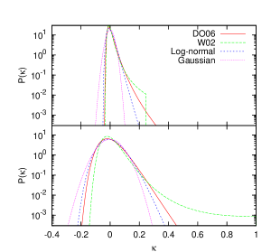
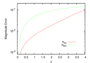
It is important to note here that, in comparing fits to simulation data, Wang et al. (2009) treated $\kappa_{\rm min}$ as a free parameter. When $\kappa_{\rm min}$ is fixed at its theoretical value from equation (11), $P_{\rm DO06}$ was, in fact, found to under-predict the high–$\kappa$ tail of the PDF. The true PDF then lies in–between $P_{\rm DO06}$ and $P_{\rm W02}$. Besides the high–$\kappa$ tail, other issues with $P_{\rm W02}$ include discontinuities and violating flux conservation at $z\hbox to0.0pt{$<$\hss}{\lower 4.30554pt\hbox{$\sim$}}0.6$ (Zentner & Bhattacharya 2009). We therefore adopt the fitting formulae from DO6, despite their imperfect fit to the simulation data. To illustrate the differences between the various PDFs, in Figure 1, we show $P_{\rm DO02}(\kappa)$, $P_{\rm W02}(\kappa)$, a log-normal PDF, and a Gaussian PDF for sources at $z=1$ (upper panel) and $z=4$ (lower panel). The cutoff of $P_{\rm W02}(\kappa)$ at $\kappa=0.25$ is imposed in order to satisfy the constraint equation (10); $P_{\rm W02}(\kappa)$ of $z=4$ is also truncated but the truncation is outside the $\kappa$ range shown in the figure. As Figure 1 shows, $P_{\rm DO6}$ and $P_{\rm W02}$ are both skewed, and the skewness is more pronounced at lower redshift. In Figure 2, we show the r.m.s. magnitude of the intrinsic and lensing dispersions as a function of redshift. For the latter, we assumed an equal–mass binary with $M_{1}=M_{2}=3\times 10^{5}{\rm M_{\odot}}$, which is close to the best case for LISA. At $z\hbox to0.0pt{$<$\hss}{\lower 4.30554pt\hbox{$\sim$}}4$, the intrinsic dispersion is always a factor of $>$$\sim$two smaller than the lensing dispersion.

In reality, there will most likely be a wide distribution of masses and mass ratios among the BH binaries detected by LISA. These distributions are highly uncertain, and for simplicity, we avoid modeling it in this paper. When both masses are in the range of $\sim 10^{5}-10^{6}~{}\rm M_{\odot}\hskip 2.84526pt$, the variation of the intrinsic error with the mass ratio is relatively modest (within a factor of $\sim 2$; Klein et al. 2009), and the fiducial accuracies we chose are typical of these binaries. For binaries with component masses significantly outside this optimal range, the intrinsic error will be larger than assumed here, and for some events, it will therefore likely become comparable (or larger) than the lensing error. Nevertheless, for most events, we expect the lensing error to remain dominant, at least at redshifts as low as $z\sim 1$, where the differences shown in Figure 2 are nearly an order of magnitude.

Figure 3: Probability distribution of the total magnitude error of standard candles (solid [red] curve) and of standard sirens (dashed [green] curve) at $z=1$. The intrinsic errors of both standard candles and of standard sirens are assumed to have Gaussian distributions (in magnitude), with a standard deviations of 0.1 mag, and $2.88\times 10^{-3}$ mag, respectively; this Gaussian is convolved with the DO06 lensing PDF (shown separately in Figure 1).

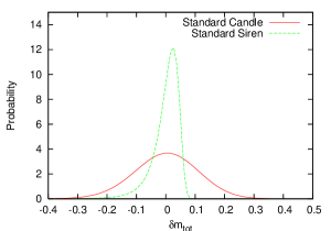
In Figure 3, we show the overall probability distribution of the magnitude error, given by the convolution of the distributions of $\delta m_{\rm int}$ and $\delta m_{\rm len}$. The solid (red) curve is for standard candles, assuming an intrinsic dispersion that is Gaussian (in magnitude) with a standard deviation of 0.1 mag (a canonical value adopted by DV06 and in many other papers; e.g. Holz & Linder 2005; Zentner et al. 2009). The dashed (green) curve is for standard sirens, again assuming a Gaussian intrinsic error distribution with a standard deviation of $2.88\times 10^{-3}$ mag. In both cases, the source is assumed to be at redshift $z=1$. As the figure shows, the overall error distribution of standard sirens remains much more skewed than that of standard candles.

We note that the intrinsic distribution of $\delta m_{\rm int}$ may well be skewed, as well. However, as long as $\delta m_{\rm int}$ is several times smaller than $\delta m_{\rm len}$, the non-Gaussianity in $\delta m_{\rm int}$ should not have a significant impact on our conclusions.

3 Likelihood analysis and Monte-Carlo simulation

We next use Monte-Carlo (MC) simulations to derive confidence intervals on the parameters inferred from mock samples of standard sirens. We follow a procedure similar to DV06, consisting of the following steps:

(1) First, we generate random redshifts for $N_{\rm event}$ standard sirens, distributed uniformly in a bin of width $\Delta z=1$, centered at redshift $z_{\rm cent}$. The number of events, $N_{\rm event}$, in each realization is varied, ranging from 40 to 2000. The lower end of this range corresponds approximately to a (pessimistic) expectation for the total number of LISA events, while the upper end corresponds to the number of SNe expected in future SN surveys such as SNAP/JDEM (allowing us to contrast standards sirens to SNe). The redshift $z_{\rm cent}$ is set at 1, 2, 3, and 4, i.e., the events are between redshift 0.5 to 4.5. At $z\hbox to0.0pt{$<$\hss}{\lower 4.30554pt\hbox{$\sim$}}0.5$, very few standard sirens are expected, and the errors from peculiar velocities become comparable to those from lensing (e.g. Kocsis et al. 2006) and would have to be included in the analysis. At $z\hbox to0.0pt{$>$\hss}{\lower 4.30554pt\hbox{$\sim$}}4.5$, the lensing PDF approaches a Gaussian shape, and the effects of non-Gaussianity become negligible, as we will see in § 4.

(2) For each event $i$, we compute the true distance modulus using equation (2). We then draw two random values of $\kappa$, one from the distribution of $P_{\rm true}(\kappa)$ and the other from $P_{\rm Gass}(\kappa)$ whose variance is set to be the same as predicted in equation (10), and convert these $\kappa$ values to $\delta m_{\rm len}$. We also draw a random $\delta m_{\rm int}$ from a Gaussian distribution with zero mean and variance $\sigma_{\rm int}$.

(3) We add $\delta m_{\rm int}$ and $\delta m_{\rm len}$ to $m_{0}$ to form two sets of mock data, ($z_{i}$, $m_{i}$), corresponding to the two choices of the convergence PDF.

(4) We then perform two separate likelihood analyses on the mock data, assuming the convergence PDF, either true or Gaussian, is known. The distribution of $\delta m_{\rm int}$ is then convolved with that of $\delta m_{\rm len}$ to obtain the PDF of the total error, $P_{\rm tot}$. In this analysis, in difference from DV06, we assume that $\sigma_{\rm int}$ is known and is fixed at the “correct” value (i.e. the same value used in step (2) above to generate the mock sample). As mentioned above, in our case, the intrinsic dispersion is sub-dominant compared to the lensing dispersion, and we therefore do not expect marginalizing over this intrinsic dispersion will modify our results.

(5) In each analysis, we vary either one or two cosmological parameters, and find the parameter value(s), $p^{\rm max}$, that maximizes the likelihood $\cal{L}$, or equivalently minimizes the quantity $\Xi\equiv-2{\rm ln}\cal{L}$. For a normalized $P_{\rm tot}$,

$$\Xi\equiv-2{\rm ln}{\cal{L}}=-2\sum_{i}{\rm ln}P_{\rm tot}(m_{i}-m_{0}(z_{i})),$$ (14)

where terms independent of cosmology have been omitted (Marshall et al. 1983). In the limit of Gaussian probability distribution $P_{\rm tot}$, $-2{\rm ln}\cal{L}$ becomes similar to the usual $\chi^{2}$ statistic.

6) We repeat the steps (1)-(5) 1000 times to produce two distributions of $p^{\rm max}$, corresponding to the two distributions of $\kappa$.

7) Finally, we evaluate the effects of the convergence PDF on the cosmological constraints by comparing these two distributions of $p^{\rm max}$.

The above approach allows us to quantify the impact of the non-Gaussian shape of the convergence PDF on the distribution of the parameter estimates. It is useful to contrast here the above approach to some others that are often used in the literature to forecast parameter errors. The Fisher-matrix formalism (Tegmark et al. 1997) is commonly adopted when the number of parameters to be estimated simultaneously is too large. This method assumes that the likelihood function is Gaussian, both as a function of the parameters to be estimated and as a function of the observables. In the present case, both of these assumptions are false (our results will be explicitly compared to those from a Fisher matrix below). Another common practice is to compute the likelihood, as a function of the parameters, around a single realization of the mock data – usually, either the most likely realization (see, e.g. Figure 6 in Holz & Hughes 2005), or in a “typical” realization (see, e.g., DV06). This avoids the assumption that the likelihood is Gaussian in the parameters, but does not fully capture the non-Gaussian shape of the distribution as a function of the observables.

In the context of SNe, Holz & Linder (2005) have used full Monte Carlo simulations to quantify the impact of lensing on the distribution of the inferred best–fit parameters, similar to our procedure above. Because of the large intrinsic dispersion of the SNe, lensing is less important to begin with, and the effect of the non-Gaussianity is also relatively modest (see their Figures 8 and 9). As far as we are aware, the same approach of using full Monte Carlo simulations have not been used to study the impact of lensing for standard sirens, for which the intrinsic dispersion is smaller, and for which the effects of lensing, as well as of non-Gaussianities, are more important.

4 Results and Discussion

4.1 Sensitivity to a single cosmological parameter

We begin by investigating the sensitivity of standard sirens to a single parameter. We focus on the degradation caused by lensing, and how this degradation is affected (hopefully, mitigated) by the non-Gaussian shape of the lensing PDF and by its dependence on cosmological parameters.

Figure 4: Distributions of $\Omega_{m}$ that maximize the likelihood. The solid [red] curve, and the dashed [blue] curves are the distributions when $P_{\rm true}(\kappa)$ and $P_{\rm Gass}(\kappa)$ are used, respectively. The shaded [green] region also shows the distribution for $P_{\rm true}(\kappa)$, but with the PDF fixed using the fiducial values of the cosmological parameters. The vertical dotted lines in this and following similar figures indicate the fiducial value of the cosmological parameter being constrained. The number of events in each realization is 40.

Figure 5: Distributions of best–fit $w$ values when the true (solid [red] curve) and Gaussian (dashed [blue] curve) PDF are used in the likelihood analysis. 1000 mock samples are generated with 40 events in each realization, distributed randomly in redshift within a bin centered at $z_{\rm cent}=1$, 2, 3 or 4, as labeled. As in Figure 4, the shaded [green] region shows results when the lensing PDF artificially uses the fixed values of the fiducial cosmological parameters.

4.1.1 Matter density $\Omega_{m}$

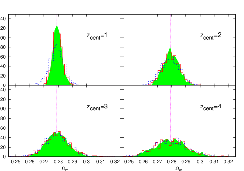
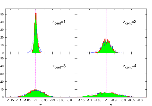
In the first example, we study the constraints on $\Omega_{m}$ while other parameters are held fixed at their fiducial values. The number of events in each realization is 40, and $z_{\rm cent}$ is set either at 1, 2, 3, or 4. The distributions of best–fit $\Omega_{m}$ values are shown in Figure 4, where the solid (red) curves and dashed (blue) curves correspond to the results when $P_{\rm true}(\kappa)$ and $P_{\rm Gass}(\kappa)$ are used in the likelihood analysis, respectively. The shaded (green) region also shows the distribution for $P_{\rm true}(\kappa)$, but with the PDF fixed using the fiducial values of the cosmological parameters. The true (fiducial) $\Omega_{m}$ is indicated by the vertical dotted lines.

The parameters of these distributions are summarized quantitatively in Table (1), which lists the peak, 68% and 95% errors of best–fit $\Omega_{m}$ and the ratios of the errors resulting from the two different assumptions about the convergence PDF (Gaussian vs. non-Gaussian). The second to last column shows the degradation due to the lensing, indicated by the ratio of 68% errors with and without lensing. For a comparison of constraining power of individual standard sirens and that of SNe Ia, the last column of Table (1) shows how many standard sirens need to be observed in each redshift bin in order to obtain the same constraints on $\Omega_{m}$ as two thousand SNe Ia at redshifts between 0.5 and 1.5. Within the parentheses are the corresponding numbers of events but in the hypothetical case that lensing is either absent or can be perfectly corrected for. In particular, an event in the first redshift bin on average has cosmological constraining power similar to $2000/114\approx 18$ SNe Ia.

Several interesting conclusions can be drawn from Figure 4 and Table 1. First, consistent with previous works, our results show that lensing severely degrades the constraints from standard sirens, and that this degradation is worse than for SNe Ia, due to the small intrinsic dispersion of standard sirens. At $z\sim 1$, lensing increases the 68% error by a factor of 4.71 for standard sirens, while only by 25% for SNe Ia. We also note that the best–fit values of $\Omega_{m}$ are essentially unbiased; this is simply because we have assumed that the shape of the lensing PDF is known ab–initio (we will relax this assumption in § 4.4 below).

Second, the constraints on $\Omega_{m}$ become worse as $z_{\rm cent}$ increases. This is because both the intrinsic and the lensing dispersions rapidly increase with redshift, as shown in Figure (2). When the number of events in a realization is fixed, the error on $\Omega_{m}$ is roughly proportional to the total dispersion of the measured distance modulus,

$$\delta\Omega_{m} \sim \delta m\left|\frac{dm}{d\Omega_{m}}\right|^{-1}\propto\delta m\left|\frac{1}{d_{L}}\frac{dd_{L}}{d\Omega_{m}}\right|^{-1}$$

$$\sim 2\Omega_{m}\delta m.$$

In the above, we have used the approximation $H(z)\approx H_{0}\sqrt{\Omega_{m}(1+z)^{3}}~{}(z\hbox to0.0pt{$>$\hss}{\lower 4.30554pt\hbox{$\sim$}}1)$, which allows us to move $\Omega_{m}$ out of the integral of $d_{L}$, and cancel the redshift dependence. Taking the values of $\sigma_{\rm true}$ in Table (1), and using the scaling that the error on a cosmological parameter is inversely proportional to the square root of the number of events, our results show that an event at $z=1$ has roughly the same contribution in constraining $\Omega_{m}$ as $(1.14\times 10^{-2}/3.49\times 10^{-3})^{2}\approx 11$ events at $z=4$.

The third and most interesting conclusion is that the constraints in the true PDF case are tighter than those in the Gaussian PDF case. The difference is as large as $\sim 50\%$ in the lowest redshift bin, where the true PDF is the most skewed and is furthest from a Gaussian shape, as clearly seen in Figure 1. This illustrates the importance of the shape of the convergence PDF, which, if not appropriately treated, could result in a biased estimate of the constraints. For example, the popular Fisher matrix technique, as we have checked, gives constraints on $\Omega_{m}$ that are very close to our Gaussian case. For any attempts of correcting for lensing on a case-by-case basis, this means that not only the variance, but the full shape of the PDF needs to be considered in the analysis, in order to evaluate the gain from such corrections. In general, these results are good news for the prospects of using standard sirens in cosmology, as the degradation from lensing is somewhat less severe than estimated from the variance alone. We also note, however, that the benefits of the non-Gaussianities largely disappear at redshifts beyond $z\hbox to0.0pt{$>$\hss}{\lower 4.30554pt\hbox{$\sim$}}2$, where the lensing PDF is closer to a Gaussian.

4.1.2 Dark energy equation of state $w$

We have also run MC simulations in which we varied the dark energy equation of state parameter $w$, while holding all other parameters fixed. The results are shown in Table (2) and Figure 5. The mock survey parameters are the same as in Table 1. The results are qualitatively similar to those in the case of $\Omega_{m}$. The benefits of the non-Gaussian shape are, however, somewhat larger, with the degradation due to lensing smaller by up to $\sim 80\%$ (in the lowest redshift bin) compared to the Gaussian case. We also note that the errors on $w$ have a steeper redshift dependence than those of $\Omega_{m}$. An event at $z=1$ has a constraining power on $w$ equivalent to $(6.83\times 10^{-2}/8.08\times 10^{-3})^{2}\approx 71$ events at $z=4$, compared to $\sim 11$ for $\Omega_{m}$. The transition from cosmic deceleration to acceleration happens at $z\sim 1$; events at this redshift are therefore especially sensitive probes of dark energy.

Table 1: The peak position ($\nu$) and the $68\%$ and $95\%$ confidence levels for the distribution of the best-fit $\Omega_{m}$ when the convergence PDF is assumed to be Gaussian (denoted by the subscript “Gass”) and when it is assumed to follow the non–Gaussian DO06 distribution (denoted by the subscript “true”). The ratios of the 68% errors in these two cases is also shown. Each realization generates a mock sample of 40 standard sirens, distributed uniformly in redshift within a width $\Delta z=1$, centered at $z_{\rm cent}=$ 1, 2, 3, or 4. The second to last column shows the degradation caused by lensing by comparing the 68% errors with and without lensing effects. The last column lists the number of standard sirens that would have similar constraining power (evaluated using the 68% error) as 2000 SNe Ia uniformly distributed between redshift 0.5 and 1.5. Within the parentheses is the corresponding number of events in the absence of lensing or with the lensing effects perfectly corrected.

	Gaussian PDF			True PDF
$z_{\rm cent}$	$\nu_{\rm Gass}$	$\sigma_{68,\rm Gass}$	$\sigma_{95,\rm Gass}$	$\nu_{\rm true}$	$\sigma_{68,\rm true}$	$\sigma_{95,\rm true}$	$\frac{\sigma_{68,\rm Gass}}{\sigma_{68,\rm true}}$	$\frac{\sigma_{95,\rm Gass}}{\sigma_{95,\rm true}}$	$\frac{\sigma_{68,\rm True}}{\sigma_{68,\rm nolens}}$	$N_{\rm SN}$
1	0.279	$5.22\times 10^{-3}$	$1.06\times 10^{-2}$	0.279	$3.49\times 10^{-3}$	$7.11\times 10^{-3}$	1.50	1.49	4.71	$1.14\times 10^{2}(8)$
2	0.279	$7.06\times 10^{-3}$	$1.42\times 10^{-2}$	0.279	$6.24\times 10^{-3}$	$1.26\times 10^{-2}$	1.13	1.12	4.57	$3.65\times 10^{2}(27)$
3	0.279	$8.60\times 10^{-3}$	$1.73\times 10^{-2}$	0.279	$8.52\times 10^{-3}$	$1.74\times 10^{-2}$	1.01	0.99	3.00	$6.80\times 10^{2}(118)$
4	0.285	$1.14\times 10^{-2}$	$2.27\times 10^{-2}$	0.276	$1.14\times 10^{-2}$	$2.31\times 10^{-2}$	1.00	0.98	1.83	$1.21\times 10^{3}(565)$

t

Table 2: Peak, 68% and 98% errors of best–fit $w$ values, for different assumptions about the convergence PDF, as in Table 1. The ratios of the errors for the different PDFs are also shown. Each realization includes 40 events.

	Gaussian PDF			True PDF
$z_{\rm cent}$	$\nu_{\rm Gass}$	$\sigma_{68,\rm Gass}$	$\sigma_{95,\rm Gass}$	$\nu_{\rm true}$	$\sigma_{68,\rm true}$	$\sigma_{95,\rm true}$	$\frac{\sigma_{68,\rm Gass}}{\sigma_{68,\rm true}}$	$\frac{\sigma_{95,\rm Gass}}{\sigma_{95,\rm true}}$
1	-1.000	$1.43\times 10^{-2}$	$2.94\times 10^{-2}$	-1.000	$8.08\times 10^{-3}$	$1.66\times 10^{-2}$	1.78	1.77
2	-0.994	$3.01\times 10^{-2}$	$6.06\times 10^{-2}$	-1.006	$2.33\times 10^{-2}$	$4.73\times 10^{-2}$	1.29	1.28
3	-1.000	$4.76\times 10^{-2}$	$9.67\times 10^{-2}$	-1.000	$4.31\times 10^{-2}$	$8.85\times 10^{-2}$	1.11	1.09
4	-0.964	$7.32\times 10^{-2}$	$1.47\times 10^{-1}$	-1.024	$6.83\times 10^{-2}$	$1.38\times 10^{-1}$	1.07	1.06

4.1.3 Power spectrum normalization $\sigma_{8}$

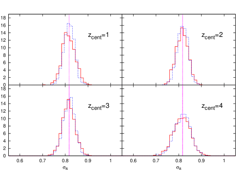
We also studied $\sigma_{8}$, which is different from $\Omega_{m}$ and $w$ in that $\sigma_{8}$ has no effect on the mean distance modulus, and therefore could not be as tightly constrained by LISA alone. To obtain good constraints (for numerical convenience), four hundred events are generated in each realization, and the results are shown in Figure 6 and Table (3). Note that constraints on $\sigma_{8}$, as opposed to those on $\Omega_{m}$ and $w$, have only a very mild dependence on redshift: the 68% errors are $\approx 0.025$ at $z=1,2$ and 3 for the case of the Gaussian distribution. This result could be understood by the following argument. First, we see from equation (2) that $\sigma^{2}_{\kappa}\propto\Delta^{2}(k,z)\propto\sigma_{8}^{2}$, of which the latter proportionality is only approximate because of nonlinear effects. This yields

$$\frac{\delta\sigma_{8}^{2}}{\sigma_{8}^{2}}=\frac{\delta\sigma^{2}_{\kappa}}{\sigma^{2}_{\kappa}}=\frac{(2/N_{\rm event})^{1/2}\sigma^{2}_{\kappa}}{\sigma^{2}_{\kappa}}=(2/N_{\rm event})^{1/2}\approx 0.071,$$ (16)

independent of redshift. When estimated from equation (16) instead, $\delta\sigma_{8}\approx\delta\sigma_{8}^{2}/2\approx 0.0236$, which is only slightly lower than the values from the numerical calculation; the small difference can be attributed to the intrinsic dispersion.

Another important difference is that non–Gaussianities degrade, rather than mitigate the lensing errors on $\sigma_{8}$, compared to the Gaussian PDF case – by $\sim 20\%$ in the lowest redshift bin. This is in contrast to the situation for $\Omega_{m}$ and $w$, for which non–Gaussianities tighten the constraints. The reason for this finding will be investigated in § 4.3 below.

Figure 6: Distributions of best–fit $\sigma_{8}$ values in 1000 Monte–Carlo realizations when the true (solid [red] curve) and a Gaussian (dashed [blue] curve) PDF are used in the likelihood analysis. 400 events are generated in each realization, in a redshift bin centered at $z_{\rm cent}=1$, 2, 3, or 4, as labeled.

Table 3: Same as Table (2), except that $\sigma_{8}$ is being constrained and each realization produces 400 events.

	Gaussian PDF			True PDF
$z_{\rm cent}$	$\nu_{\rm Gass}$	$\sigma_{68,\rm Gass}$	$\sigma_{95,\rm Gass}$	$\nu_{\rm true}$	$\sigma_{68,\rm true}$	$\sigma_{95,\rm true}$	$\frac{\sigma_{68,\rm Gass}}{\sigma_{68,\rm true}}$	$\frac{\sigma_{95,\rm Gass}}{\sigma_{95,\rm true}}$
1	0.814	$2.42\times 10^{-2}$	$4.65\times 10^{-2}$	0.814	$2.93\times 10^{-2}$	$5.76\times 10^{-2}$	0.83	0.81
2	0.814	$2.48\times 10^{-2}$	$4.76\times 10^{-2}$	0.814	$2.78\times 10^{-2}$	$5.32\times 10^{-2}$	0.89	0.89
3	0.814	$2.64\times 10^{-2}$	$5.21\times 10^{-2}$	0.814	$2.83\times 10^{-2}$	$5.74\times 10^{-2}$	0.93	0.91
4	0.826	$3.56\times 10^{-2}$	$7.01\times 10^{-2}$	0.814	$3.78\times 10^{-2}$	$7.45\times 10^{-2}$	0.94	0.94

4.2 Information from the parameter-dependence of the PDF

As explained above, we have included two effects about the lensing PDF in our analysis: (i) its non-Gaussian shape, and (ii) its dependence on cosmological parameters. It is important to clarify which of these two effects was responsible for the improvement in the constraints on $\Omega_{m}$ and $w$, relative to the case when the lensing PDF is Gaussian and is considered pure noise (i.e. with no parameter–dependence). Assuming a Gaussian PDF and employing the Fisher matrix method, Zentner & Bhattacharya (2009), find that the dispersion of SNe Ia moduli can help break degeneracies between dark energy parameters. However, the non-Gaussian, high-convergence tail of the lensing PDF has been shown explicitly to contain cosmological information, whose statistical accuracy in an all-sky map is competitive with other cosmological probes (Wang et al. 2009).

We perform two tests in order to establish which of the two effects is more important. First, we artificially fix the shape of the PDF with the fiducial values of cosmological parameters throughout the analysis. The results of this academic exercise are shown in Figures 4 and 5 by the shaded regions. This brings only a marginal change in the distributions of the best–fit values compared to the fiducial case, showing that the effects of the true lensing PDF come primarily through its non-Gaussianity, rather than through its cosmology–dependence.

This conclusion is confirmed by a second test, in which we artificially fix the distance modulus, and re–derive constraints on $\Omega_{m}$. We find that the constraints in this case become by about an order of magnitude worse. A closer investigation shows that for $\Omega_{m}$, the cosmological dependence of the PDF, in fact, slightly harms the constraints, while for $w$, it slightly improves the constraints. The fact that the cosmological dependence of the PDF harms the constraints on $\Omega_{m}$ must also be caused by the non-Gaussian shape of the PDF. This is because for a Gaussian PDF, it could be argued (e.g. using the Fisher matrix) that additional information can only improve the sensitivity to a parameter (by increasing the absolute value of the corresponding element in the Fisher matrix). We have verified by numerical calculation that for a Gaussian PDF, the cosmological dependence indeed improves constraints on both $\Omega_{m}$ and $w$, in agreement with this argument.

4.3 Why does non-Gaussianity of the PDF affect the constraints?

In this section, we discuss why the parameter constraints are affected by the shape of the convergence PDF. To illustrate this, we consider a quantity $\xi$, defined as,

$$\xi\equiv\frac{d\langle\Xi\rangle}{d\delta m_{\rm tot}}=-2P_{\rm tot}(\delta m_{\rm tot}){\rm ln}P^{\prime}_{\rm tot}(\delta m^{\prime}_{\rm tot}),$$ (17)

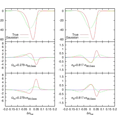
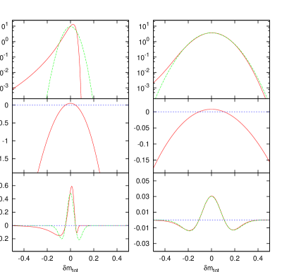
where $\langle\Xi\rangle$ is the expectation value of $\Xi$ for one event. In equation (17), the factor $P_{\rm tot}(\delta m_{\rm tot})$, computed with the true convergence PDF and with the fiducial values of the cosmological parameters, is the probability that an event has a (true) total deviation of $\delta m_{\rm tot}$. The factor $-2{\rm ln}P^{\prime}_{\rm tot}(\delta m^{\prime}_{\rm tot})$, computed with the convergence PDF adopted for the likelihood analysis (i.e. either a Gaussian or the true PDF) and with the varying cosmological parameters, represents the contribution to $\Xi$ from a single event with this $\delta m_{\rm tot}$. Note that the residual distance modulus inferred in a test cosmology, $\delta m^{\prime}_{\rm tot}$, differs from the true residual $\delta m_{\rm tot}$, since the luminosity distances in the two cosmologies are different. In the top left panel of Figure 7, we show $\xi$ at $z=1$ as a function of the true residual $\delta m_{\rm tot}$, where $\Omega_{m}$ is set at its fiducial value.

The change in $\xi$ when $\Omega_{m}$ is varied, $\Delta\xi$, is shown in the left middle and left bottom panels, in which $\Omega_{m}$ is decreased or increased by $\sigma_{\rm 68,Gass}$ ($=5.22\times 10^{-3}$, see Table 1), respectively. The main effect of changing $\Omega_{m}$ is to shift the measured residual $\delta m^{\prime}_{\rm tot}$ away from its true value of $\delta m_{\rm tot}$, producing wave–like shapes in the curves $\Delta\xi=\Delta\xi(\delta m_{\rm tot})$. For example, assuming an $\Omega_{m}$ larger than its fiducial value (bottom panel) increases the apparent residuals $\delta m^{\prime}_{\rm tot}$ by reducing the distances ($d_{L}(z)$) and therefore reducing $m_{0}$. In other words, the source is inferred to be too close, and the magnification is inferred (statistically) to be smaller than the correct value. This corresponds to a reduced probability and increased $\xi$ at large positive $\delta m_{\rm tot}$ where the $P_{\rm tot}(\delta m_{\rm tot})$ decreases with $\delta m_{\rm tot}$ (i.e. if the source was already strongly demagnified; see the dashed curve in Figure  3). Conversely, it results in an enhanced probability and a decreased $\xi$ at negative $\delta m_{\rm tot}$ (if the source was strongly magnified, it is inferred to need less magnification, which has a larger probability). The increase of $\xi$ at mildly positive $\delta m_{\rm tot}$ and the decrease at mildly negative $\delta m_{\rm tot}$ are both stronger in the case of true PDF. This is because near $\delta m_{\rm tot}\approx 0$, the contribution to $\xi$ is a much steeper function of $\delta m_{\rm tot}$ for the true PDF, as seen clearly in the top panel. Indeed, the change of $\Xi$, i.e. the integral of $\Delta\xi$, is correspondingly also larger in the case of the true PDF, leading to an improved constraint on $\Omega_{m}$.

The fact that the sharp features of the non-Gaussian lensing PDF near its peak help tighten the sensitivity to $\Omega_{m}$ may be surprising, since they are in contrast with the more widely discussed, detrimental, effects of long non-Gaussian tails. For example, the mean of $N$ numbers, generated from a non–Gaussian distribution, convergences less rapidly (than $1/\sqrt{N}$) to the correct value, due to such shallow, non-Gaussian tails. However, when one fits the entire shape of the distribution (rather than utilizing just the mean), then, intuitively, the benefits of sharp features are not surprising. For example, one can envision a hypothetical, picket-fence-shaped distribution with the same r.m.s. as a smooth Gaussian. It is easy to see that if the picket-fence pattern shifts with a parameter, then this parameter can be arbitrarily tightly constrained, in the limit that the picket-fence shapes become arbitrarily sharp Dirac $\delta$–functions.

The right panels of Figure 7 show the same quantities as in the left panel, except for $\sigma_{8}$. Unlike $\Omega_{m}$, $\sigma_{8}$ does not change the mean $\delta m^{\prime}_{\rm tot}$. As a result, in the Gaussian case, the curves of $\Delta\xi$ are strictly symmetric about $\delta m_{\rm tot}=0$. The middle right and the bottom right panels show that the non–Gaussianity again enhances the sensitivity to $\sigma_{8}$ near the peak (for modest demagnifications), whereas $\xi$ in the tail of the true PDF becomes relatively insensitive to the change in $\sigma_{8}$. Overall, this loss of sensitivity in the tails is the larger effect, and it renders $\Delta\Xi$ smaller than the Gaussian case. This explains why the constraints on $\sigma_{8}$ becomes worse when the true PDF is used.

Figure 7: The top panels show the contribution to $\xi$ (a $\chi^{2}$–like quantity; see text for the definition) at $z=1$ from events with different $\delta m_{\rm tot}$ (the deviation in the distance modulus from that in a homogeneous universe). The middle and bottom panels show the change in the $\xi$–contributions when the parameter is reduced or increased by one standard deviation $\sigma_{\rm 68,Gass}$. The left and right panels are for $\Omega_{m}$ and $\sigma_{8}$, respectively.

4.4 How important is it to know the correct shape of the PDF?

Table 4: The peak of the maximum-likelihood estimator of $\Omega_{m}$ and its 68% and 95% errors when the mock data, produced using the “true” PDF, is fitted by erroneously using either a Gaussian or a log-normal magnification PDF. The setup is otherwise the same as in Table 1.

	Gaussian PDF					Log-normal PDF
$z_{\rm cent}$	$\nu_{\rm Gass}$	$\sigma_{68,\rm Gass}$	$\sigma_{95,\rm Gass}$	$\frac{\sigma_{68,\rm Gass}}{\sigma_{68,\rm true}}$	$\frac{\sigma_{95,\rm Gass}}{\sigma_{95,\rm true}}$	$\nu_{\rm log}$	$\sigma_{68,\rm log}$	$\sigma_{95,\rm log}$	$\frac{\sigma_{68,\rm log}}{\sigma_{68,\rm true}}$	$\frac{\sigma_{95,\rm log}}{\sigma_{95,\rm true}}$
1	0.277	$6.05\times 10^{-3}$	$1.32\times 10^{-2}$	1.74	1.86	0.282	$3.73\times 10^{-3}$	$7.74\times 10^{-3}$	1.07	1.09
2	0.279	$7.83\times 10^{-3}$	$1.68\times 10^{-2}$	1.25	1.33	0.279	$6.47\times 10^{-3}$	$1.35\times 10^{-2}$	1.04	1.07
3	0.279	$9.50\times 10^{-3}$	$1.94\times 10^{-2}$	1.12	1.11	0.279	$8.78\times 10^{-3}$	$1.77\times 10^{-2}$	1.03	1.02
4	0.277	$1.22\times 10^{-2}$	$2.31\times 10^{-2}$	1.07	1.00	0.274	$1.16\times 10^{-2}$	$2.34\times 10^{-2}$	1.03	1.01

Table 5: Same as Table 4, except that $w$ is being constrained.

	Gaussian PDF					Log-normal PDF
$z_{\rm cent}$	$\nu_{\rm Gass}$	$\sigma_{68,\rm Gass}$	$\sigma_{95,\rm Gass}$	$\frac{\sigma_{68,\rm Gass}}{\sigma_{68,\rm true}}$	$\frac{\sigma_{95,\rm Gass}}{\sigma_{95,\rm true}}$	$\nu_{\rm log}$	$\sigma_{68,\rm log}$	$\sigma_{95,\rm log}$	$\frac{\sigma_{68,\rm log}}{\sigma_{68,\rm true}}$	$\frac{\sigma_{95,\rm log}}{\sigma_{95,\rm true}}$
1	-1.003	$1.36\times 10^{-2}$	$2.62\times 10^{-2}$	1.68	1.57	-0.991	$8.15\times 10^{-3}$	$1.75\times 10^{-2}$	1.01	1.05
2	-1.006	$2.90\times 10^{-2}$	$6.03\times 10^{-2}$	1.25	1.27	-1.000	$2.36\times 10^{-2}$	$4.94\times 10^{-2}$	1.02	1.05
3	-1.012	$4.89\times 10^{-2}$	$9.71\times 10^{-2}$	1.14	1.10	-1.000	$4.37\times 10^{-2}$	$8.93\times 10^{-2}$	1.02	1.01
4	-1.000	$7.23\times 10^{-2}$	$1.46\times 10^{-1}$	1.06	1.05	-0.988	$6.92\times 10^{-2}$	$1.39\times 10^{-1}$	1.01	1.00

Table 6: Same as Table 4, except that $\sigma_{8}$ is constrained and there are 400 events in each realization.

	Gaussian PDF					Log-normal PDF
$z_{\rm cent}$	$\nu_{\rm Gass}$	$\sigma_{68,\rm Gass}$	$\sigma_{95,\rm Gass}$	$\frac{\sigma_{68,\rm Gass}}{\sigma_{68,\rm true}}$	$\frac{\sigma_{95,\rm Gass}}{\sigma_{95,\rm true}}$	$\nu_{\rm log}$	$\sigma_{68,\rm log}$	$\sigma_{95,\rm log}$	$\frac{\sigma_{68,\rm log}}{\sigma_{68,\rm true}}$	$\frac{\sigma_{95,\rm log}}{\sigma_{95,\rm true}}$
1	0.790	$5.02\times 10^{-2}$	$1.06\times 10^{-1}$	1.67	1.78	0.742	$2.53\times 10^{-2}$	$4.93\times 10^{-2}$	0.84	0.83
2	0.814	$3.68\times 10^{-2}$	$7.02\times 10^{-2}$	1.32	1.32	0.790	$2.66\times 10^{-2}$	$5.04\times 10^{-2}$	0.95	0.95
3	0.814	$3.25\times 10^{-2}$	$6.47\times 10^{-2}$	1.15	1.13	0.802	$2.76\times 10^{-2}$	$5.56\times 10^{-2}$	0.97	0.97
4	0.826	$4.13\times 10^{-2}$	$8.06\times 10^{-2}$	1.09	1.08	0.814	$3.80\times 10^{-2}$	$7.47\times 10^{-2}$	1.00	1.00

Our results above show that the shape of the lensing PDF has a non-negligible effect on the parameter constraints. However, the analysis above has assumed that the shape of the lensing PDF is precisely known.

A related question of interest, therefore, is: how accurately do we need to know the lensing PDF, in order to avoid either a bias in the inferred parameters, or a mis-estimation of its confidence levels?

In order to investigate this issue, we here create mock data-sets with the “true” lensing PDF from DO06, but we fit them using “wrong” PDFs. The two “wrong” PDFs we chose are a Gaussian (representing an extremely wrong case), and a log-normal distribution (which represents a more reasonable estimate of the current uncertainty about the convergence PDF). The results for $\Omega_{m}$, $w$ and $\sigma_{8}$ are shown in Tables 4–6.

Tables 4 shows that the maximum–likelihood estimate (MLE) of $\Omega_{m}$ remains essentially unbiased: the MLE distribution peaks at values that are offset from the true value of $\Omega_{m}=0.279$ by at most $\approx 1/3$rd of the 68% confidence level. This result is in agreement with DV06, and is not surprising, since the peak of the best–fit $\Omega_{m}$ distribution is determined primarily by the luminosity distance (or the homogeneous distance modulus $m_{0}$), rather than the shape of the $\delta m$–distribution. The variance of the best–fit $\Omega_{m}$, however, becomes larger when the Gaussian or log-normal PDF is used in the likelihood analysis. The difference in the lowest redshift bin is $\sim 80\%$ for a Gaussian PDF, but only $\sim 10\%$ for the log–normal PDF. This question has also been investigated in the context of SNe Ia by DV06, who found that the variance is almost unchanged. We have confirmed their conclusion by running a similar Monte-Carlo simulation for a mock SNe Ia survey. The reason why the constraints on $\Omega_{m}$ from standard sirens, in contrast to standard candles, are obviously affected by the choice of the convergence PDF, is the large skewness (seen in Fig. 3) in the error distribution of standard sirens (see more explicit demonstration of this point below). From Table 4, it is also clear that the improvement of the constraints on $\Omega_{m}$ decreases with increasing source redshift. This feature could also be explained by the decrease in the skewness of the distribution with increasing source redshift. Here, the change is not driven by the intrinsic dispersion, but by the lensing dispersion. As we show in Figure 1, the convergence PDF is more skewed at low redshift, making the effect of non-Gaussianity more prominent.

The conclusions for $w$ are qualitatively very similar, except that the differences caused by the “wrong” PDFs are smaller, as shown in Table 5. In fact, the constraints with the log-normal PDF are almost identical to those from the “true” PDF, with a negligible bias, and with an overestimate of the 68% error by only 2%. We expect these qualitative conclusions, from the examples of $\Omega_{m}$ and $w$, to remain valid for other parameters such as the Hubble constant $h$, or the dark energy equation of state evolution parameter $dw/dz$, whose impact is primarily through $d_{L}(z)$, rather than the shape of the lensing PDF.

Figure 8: Distributions of the best–fit $\sigma_{8}$ values, obtained by fitting the “true” magnification PDF with erroneous Gaussian PDFs, in two Monte-Carlo simulations that only differ in the size of the intrinsic scatter. The left (right) panel shows the results when the intrinsic scatter is typical of standard sirens (standard candles). Two thousand events are generated in each realization. Note that $\sigma_{8}$ is negatively biased for standard sirens, while it is positively biased for SNe (see text and Figure 9 for an explanation of this result).

Interestingly, as shown in Table 6, for $\sigma_{8}$, the erroneous use of the Gaussian PDF also degrades the constraints, while the log-normal PDF gives rise to better constraints, but causes a clear negative bias. At the lowest redshift, the bias is $\sim 0.07$, exceeding the forecast 68% constraint. The still larger, and positive, bias of $\sigma_{8}$ for the Gaussian PDF seen in DV06 was not found in our calculations; instead, the peak is slightly negatively biased in the lowest redshift bin (we find the mean, however, is almost unbiased).

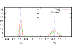
Investigations of the seeming inconsistency with DV06 revealed, initially to our own surprise, that the sign of the $\sigma_{8}$–bias is affected by the size of the intrinsic scatter, in addition to the skewness of the lensing PDF. To illustrate this point, in Figure 8 we plot the distributions of the best–fit $\sigma_{8}$ from two Monte-Carlo simulations that only differ in the amount of the intrinsic scatter – the left panel assumes the intrinsic dispersion of a typical standard siren, while the right panel assumes that of a typical standard candle ($\sigma_{\rm int}=0.1$, as before). As the right panel of this figure shows, in addition to increasing the variance of the inferred $\sigma_{8}$ distribution, a larger intrinsic dispersion also shifts the peak position to a higher value, in the case of the Gaussian PDF. This positive bias in the SN sample has a value of $\Delta\sigma_{8}\approx 0.017$.

To understand why the $\sigma_{8}$–bias changes sign as the intrinsic scatter is increased, we again consider the quantity $\xi$ and its dependence on $\sigma_{8}$. In the bottom panels of Figure 9, we show $\Delta\xi$ ($\equiv\xi(\sigma_{8}=0.834)-\xi({\rm fiducial}~{}\sigma_{8}=0.817)$, solid curves) for the case of the erroneous Gaussian PDF; the left and right panels are again for standard sirens and for SNe Ia, respectively. In agreement with the results of the Monte-Carlo simulations, $\Delta\Xi$ from the integration of $\Delta\xi$ is negative for SNe Ia, meaning the bias is positive, while $\Delta\Xi$ for standard sirens is positive, consistent with no bias. The top and bottom panels show $P_{\rm tot}(\delta m_{\rm tot})$ and $\Delta(-2{\rm ln}P^{\prime}_{\rm tot}(\delta m^{\prime}_{\rm tot}))$, the two multiplicative factors comprising $\Delta\xi$. For comparison, we also show, by the dashed curves, the same quantities in a “true Gaussian” case, where the “true” convergence PDF (in addition to the PDF employed in the likelihood analysis) is assumed to be Gaussian, and therefore the estimate of $\sigma_{8}$ should be unbiased.

Compared with the Gaussian “true” distribution, the skewed “true” distribution produces a much higher probability of strongly magnified events (solid curves in the top panels). These events contribute negative $\Delta\xi$, i.e., they favor larger $\sigma_{8}$ values (the solid curve is largely below the dashed curve at $\delta m_{\rm tot}<0$). This is the effect that dominates in the case of SNe, as already argued by DV06. However, when the intrinsic dispersion is small, this negative contribution to $\Xi$ is, in fact, balanced by the decrease of the probability at $\delta m_{\rm tot}\hbox to0.0pt{$>$\hss}{\lower 4.30554pt\hbox{$\sim$}}0$. In other words, the large $\sigma_{8}$ value that is favored by the events in the strongly magnified tail, is even more strongly disfavored by the lack of corresponding mildly demagnified events – leading to an overall negative bias in $\sigma_{8}$. In the SN case, when the intrinsic dispersion is large, there is no longer a lack of mildly demagnified events to be disfavored, because the expected number of these events is still dominated by the intrinsic scatter, and is insensitive to $\sigma_{8}$ — the net effect, in this case, is the positive bias in $\sigma_{8}$, driven by the highly magnified events.

Figure 9: The top panels show the probability distributions of $\delta m_{\rm tot}$ at $z=1$. The solid and dashed curves assume that the true convergence PDF follows $P_{\rm Do}$ or a Gaussian, respectively. The middle panels show the change in $-2{\rm ln}P^{\prime}_{\rm tot}(\delta m^{\prime}_{\rm tot})$ when $\sigma_{8}$ is increased from the fiducial value of 0.817 to 0.834 (the mean of $\sigma_{8}$ from SNe Ia simulations when Gaussian PDF is used in the likelihood analysis). The bottom panels show the corresponding change in the $\chi^{2}$–like quantity $\xi$. The left and right panels are for standard sirens and SNe Ia, respectively.

4.5 Varying two cosmological parameters

Figure 10: Upper panel: Contours enclosing 68% and 95% of the best–fit values on $\Omega_{m}$ and $w$ in the lowest redshift bin for the true (solid line) and Gaussian (dashed line) PDF. In each case, $10^{4}$ realizations were produced of mock samples containing 100 standard sirens, and $\Omega_{m}$ and $w$ were fit simultaneously, with all other parameters fixed at their fiducial values. Bottom left panel: Distribution of best–fit $\Omega_{m}$, marginalized over $w$. Bottom right panel: Distribution of best–fit $w$, marginalized over $\Omega_{m}$.

Figure 11: Same as Figure 10, except that $\Omega_{m}$ and $\sigma_{8}$ are being simultaneously constrained.

Table 7: The peak, 68% and 95% marginalized errors of $\Omega_{m}$ and $w$ for Gaussian and true PDFs. Each realization produces 100 events.

	Gaussian PDF			True PDF
Parameter	$\nu_{\rm Gass}$	$\sigma_{68,\rm Gass}$	$\sigma_{95,\rm Gass}$	$\nu_{\rm true}$	$\sigma_{68,\rm true}$	$\sigma_{95,\rm true}$	$\frac{\sigma_{68,\rm Gass}}{\sigma_{68,\rm true}}$	$\frac{\sigma_{95,\rm Gass}}{\sigma_{95,\rm true}}$
$\Omega_{m}$	0.280	$1.44\times 10^{-2}$	$2.87\times 10^{-2}$	0.277	$1.22\times 10^{-2}$	$2.69\times 10^{-2}$	1.18	1.07
$w$	-0.986	$3.69\times 10^{-2}$	$7.78\times 10^{-2}$	-1.000	$2.92\times 10^{-2}$	$6.18\times 10^{-2}$	1.26	1.26

Table 8: The peak, 68% and 95% marginalized errors of $\Omega_{m}$ and $\sigma_{8}$ for Gaussian and true PDFs. Each realization produces 100 events.

	Gaussian PDF			True PDF
Parameter	$\nu_{\rm Gass}$	$\sigma_{68,\rm Gass}$	$\sigma_{95,\rm Gass}$	$\nu_{\rm true}$	$\sigma_{68,\rm true}$	$\sigma_{95,\rm true}$	$\frac{\sigma_{68,\rm Gass}}{\sigma_{68,\rm true}}$	$\frac{\sigma_{95,\rm Gass}}{\sigma_{95,\rm true}}$
$\Omega_{m}$	0.280	$3.46\times 10^{-3}$	$6.92\times 10^{-3}$	0.279	$2.92\times 10^{-3}$	$6.03\times 10^{-3}$	1.19	1.15
$\sigma_{8}$	0.814	$4.64\times 10^{-2}$	$9.25\times 10^{-2}$	0.820	$7.99\times 10^{-2}$	$1.65\times 10^{-1}$	0.58	0.56

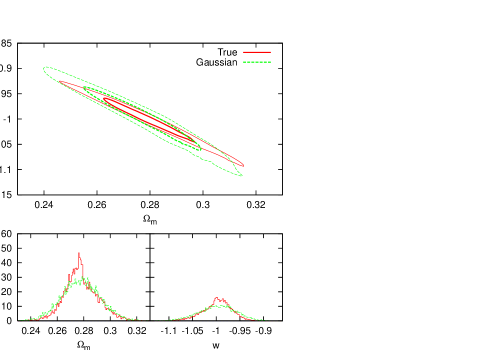
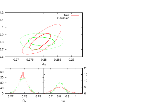
In our calculations above, we varied a single parameter, while all others were held fixed. To take into account the correlations among different cosmological parameters, we next consider simultaneous constraints on two cosmological parameters. Ideally, all of the cosmological parameters should be allowed to vary simultaneously, for a full study of correlations. Unfortunately, with our simple Monte-Carlo method, this is computationally prohibitively expensive (and would require the use of Monte Carlo Markov Chains, or a similar technique). In this study, for simplicity, we instead chose to study only two typical correlations as illustrative examples. One of the correlations, between $\Omega_{m}$ and $w$, is expected to be large, since as we have shown, both parameters draw their constraints from the mean distance modulus. The other correlation, between $\Omega_{m}$ and $\sigma_{8}$, is expected to be small, as the constraints on $\sigma_{8}$ are purely from the cosmological dependence of the shape of the convergence PDF. We focus on the lowest redshift bin of $z_{\rm cent}=1$, where the assumed shape of the convergence PDF makes the largest difference. One hundred events are generated in each realization.

The joint 2-D confidence contours and the marginalized 1-parameter distributions are plotted in Figure 10 (for simultaneous constraints on $\Omega_{m}$ and $w$) and in Figure 11 (for simultaneous constraints on $\Omega_{m}$ and $\sigma_{8}$). The values of the marginalized errors are also listed in Tables 7 and 8.

Figure 10 confirms that $\Omega_{m}$ and $w$ are strongly anti–correlated. As in the single parameter case, $\Omega_{m}$ and $w$ are both more tightly constrained with the true PDF, by 18% for $\Omega_{m}$ and 26% for $w$ (evaluated using their marginalized 68% errors). The area enclosed by the 68% (95%) contour is larger in the Gaussian PDF case by 117% (92%). The raw sensitivity to the combination of $\Omega_{m}$ and $w$ is therefore improved, by the presence of non-Gaussianity, by more than a factor of two.

Figure 11 shows that the correlation between $\Omega_{m}$ and $\sigma_{8}$ depends on the shape of the convergence PDF. With a Gaussian PDF, the parameters are almost uncorrelated, while with the true PDF, they are positively correlated. Here we offer a heuristic explanation for this positive correlation: with larger $\sigma_{8}$, the convergence dispersion is increased, making the convergence PDF more skewed, and its peak shift to lower $\kappa$; to fit the same $m_{\rm tot}$, this requires a larger $\Omega_{m}$ to compensate. The marginalized error on $\Omega_{m}$ is still smaller with the true PDF, but the difference of the 68% errors, only 19%, is considerably smaller than in the single parameter case. At the same time, the constraints on $\sigma_{8}$ are slightly more degraded than those with a Gaussian PDF. Here, the area enclosed by the 68% (95%) contour is smaller in the Gaussian PDF case by 6% (10%).

4.6 The importance of the number of events

Another interesting question to ask is: how do our results – in particular, the tightening or degradation in the constraints caused by non–Gaussianities – depend on the number of standard siren events $N_{\rm event}$? Depending on what statistic is being used, non-Gaussianities can become increasingly unimportant as $N_{\rm event}\rightarrow\infty$. This is the case, for example, when one considers the distribution of the mean magnification $\langle\delta m\rangle$ from $N_{\rm event}$ events (as is well known from the central limit theorem; see, e.g., Figure 1 in Holz & Linder 2005). This statistic, however would be relevant only if one simply ignored lensing, and performed a least-squares fit to the observed Hubble diagram. This is different from the maximum-likelihood estimator we adopted here, which includes information beyond the mean magnification, and utilizes the full shape of the PDF. In fact, we expect that the MLE has a distribution for which the non-Gaussianity does not average away in the limit of a large number of events.

In Table 9, we show the ratios of the 68% errors in the true and the Gaussian cases, when the number of events in each realization is increased and decreased, by a factor of 4, from the values adopted in § 4.1. As the table shows, the ratios are consistent with no dependence on $\sqrt{N_{\rm event}}$ (while the absolute errors, which are not shown in the table, were found to scale approximately as $\sqrt{N_{\rm event}}$). Therefore, the general conclusion of this study, that the non-Gaussian shape non-trivially affects cosmological constraints, is valid independent of $N_{\rm event}$. This also demonstrates the importance of choosing an optimal statistic: the information from the skewness in the PDF would be lost if only the mean distance modulus were used.

Table 9: The ratios of the 68% errors on the individual cosmological parameters in the true and in the Gaussian cases, when the number of events in each realization is increased or decreased by a factor of 4 relative to our fiducial choices.

$N_{\rm event}$	$\times 0.25$	$\times 1$	$\times 4$
$\Omega_{m}$	1.57	1.50	1.55
$w$	1.72	1.78	1.70
$\sigma_{8}$	0.76	0.83	0.82

4.7 The expected constraints from a LISA standard siren sample

Figure 12: A crude estimate for the number of SNe whose statistical constraining power is equivalent to that of a single standard siren. We have assumed that the magnitude errors of the two types of sources follow the same distribution, with the amplitude given by the convolution of intrinsic and lensing errors.

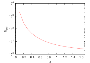
What is the actual expected error from LISA standard sirens on cosmological parameters, in the presence of lensing? Since we have not obtained these errors in the full multi–dimensional parameter space, we cannot fully answer this question. However, the same question has been studied exhaustively in the context of SNe – and, since the SNe constraints are from the same observable (the Hubble diagram), it makes sense to quote the expectations from standard sirens relative to those from a SN sample. If the magnitude errors had the same distribution for these two types of sources, with standard deviations of $\sigma_{\rm ss}$ and $\sigma_{\rm sn}$, then the statistical constraints from a single standard siren would be equivalent to that from $N_{\rm sn,1}=(\sigma_{\rm ss}/\sigma_{\rm sn})^{-2}$ SNe. Assuming a constant $\sigma_{\rm sn}\approx 0.1$ mag, and also that the lensing and intrinsic errors add in quadrature, in Figure 12 we show $N_{\rm sn,1}$. As the intrinsic errors of standard sirens approach those of SNe, their relative advantage decreases monotonically with redshift, with $N_{\rm sn,1}\approx 93\rightarrow 5.5\rightarrow 2.5$ at $z\approx 0.3\rightarrow 1\rightarrow 1.7$. (Peculiar velocities will limit the constraints from standard sirens below redshifts $z\hbox to0.0pt{$<$\hss}{\lower 4.30554pt\hbox{$\sim$}}0.3$.) The main result of this paper could be stated by saying that at $z=1$, these numbers for $N_{\rm sn}$ are increased by a factor of $1.5^{2}=2.25$ for $\Omega_{m}$, and by a factor of $1.8^{2}=3.25$ for $w$; whereas they are decreased by a factor of $0.8^{2}=0.64$ for $\sigma_{8}$. Note that while the actual numbers for $N_{\rm sn,1}$ are only crude estimates, these increases/decreases, which are due to the non–Gaussian shape of the lensing PDF, should be robust. At higher redshifts, these increases/decreases disappear.

These estimates apply to a single redshift, and to a single cosmological parameter. The constraints from an actual set of LISA standard sirens will, of course, depend on the redshift distribution of the sources. If most of the standard sirens are at high redshifts ($z\hbox to0.0pt{$>$\hss}{\lower 4.30554pt\hbox{$\sim$}}3$; e.g., in Sesana 2004) then our results suggest that there will be no significant overall improvements from non-Gaussianity for the set of events. If there are more events at low redshift, then non-Gaussianity will improve the constraints significantly. Having low-$z$ events remains a possibility (see, e.g., discussion of some of the uncertainties, and related references, in Lippai et al. 2009). Holley-Bockelmann et al. (2010) recently found, using cosmological simulations of the BH merger trees, that most LISA-detectable merger events are below $z=2$ (albeit with high mass ratios, so their intrinsic $d_{L}$ error will be worse than for the equal–mass binaries adopted here). Finally, even if most events are at $z\hbox to0.0pt{$>$\hss}{\lower 4.30554pt\hbox{$\sim$}}4$, non–Gaussianities can still improve the overall constraints when the LISA data is combined with information from still higher redshift, such as cosmic microwave background (CMB) anisotropies. Since the CMB fixes the luminosity distance at $z\approx 1,000$, the lowest–redshift standard sirens will have the longest “lever–arm” and the contribution from these events to the combined LISA+CMB constraints will be enhanced significantly (a point emphasized in a different context by Hu & Haiman 2003).

5 Conclusions

In this paper, we have shown that the sensitivity of low–redshift ($z\sim 1$) standard sirens to the parameters $\Omega_{m}$ and $w$ are tightened, by a factor of $1.5-1.8$, by the non–Gaussian shape of the lensing magnification PDF, relative to a Gaussian PDF with the same variance. When these two parameters are constrained simultaneously, the improvement of the constraints, attributable to the skewness alone, is further enhanced, owing to the correlation between the parameters. We expect similar conclusions to hold for other parameters whose constraints are driven primarily by the changes they induce in the luminosity distance $d_{L}(z)$. Interestingly, the constraint on $\sigma_{8}$, which comes from the shape of the PDF itself, is, however, degraded by a factor of $\approx 0.8$. In our study, we relied on the shape of the lensing PDF described by the fitting formulae in Das & Ostriker (2006). This shape is somewhat less skewed than the simulation results, suggesting that the improvement / degradation of the constraints has likely been underestimated.

The improvements for $\Omega_{m}$ and $w$ are comparable to those that may be available from correlations with lensing measurements on larger scales, or from directly subtracting the lensing contribution of foreground galaxies. However, these corrections from non-Gaussianities are “automatically” available, as long as the lensing PDF can be modeled ab–initio. We also found that at higher redshift, the effects from non–Gaussianity are less pronounced due to the reduced skewness of the lensing PDF. Overall, our results highlight the importance of obtaining an accurate and reliable PDF of the point–source lensing magnification, in order to realize the full potential of standard sirens as cosmological probes.

References

- [1]
- [Aldering et al. 2004] Aldering G. et al. (SNAP collaboration), 2004, preprint (astro-ph/0405232)
- [Arun et al. 2009a] Arun K. G., Mishra C. K., Van Den Broeck C., Iyer B. R., Sathyaprakash B. S., Sinha S., 2009a, Class. Quant. Grav., 26, 094021
- [2] Arun K. G. et al., 2009b, Class. Quant. Grav., 26, 094027
- [3] Cooray, A., Holz, D. E., & Huterer, D. 2006, ApJL 637, 77
- [4] Cutler, C., & Holz, D. E., 2009, Phys. Rev. D., 80, 104009
- [5] Dalal N., Holz D. E., Chen X., Frieman J. A., 2003, ApJ, 585, 11
- [6] Dalal N., Holz D. E., Hughes, S. A., & Jain, B., 2006, Phys. Rev. D, 74, id. 063006
- [7] Das S., Ostriker J. P., 2006, ApJ, 645, 1
- [8] Dodelson S., Vallinotto A., 2006, Phys. Rev. D, 74, 063515
- [9] Jönsson J., Goobar A., Mörtsell E., 2007, ApJ, 658, 52
- [10] Haiman Z., Kocsis B., Menou K., Lippai, Z., & Frei, Z. 2009, Class. Quant. Grav., 26, 094032 (2009).
- [11] Holley-Bockelmann, K., Micic, M., Sigurdsson, S., & Rubbo, L. 2010, ApJ, in press, e-print arXiv:1002.3378
- [12] Holz D. E., & Hughes S. A., 2005, ApJ, 631, 678
- [13] Holz D. E., & Linder, E. V, 2005, ApJ, 629, 15
- [14] Hu, W., & Haiman, Z. 2003, Phys. Rev. D, vol. 68, Issue 6, id. 063004
- [15] Klein A., Jetzer, P., Sereno M., 2009, Phys. Rev. D, 80, 064027
- [16] Kocsis B., Frei Z., Haiman Z., Menou K., 2006, ApJ, 637, 27
- [17] Kocsis B., Frei Z., Haiman Z., Menou K., 2007, Phys. Rev. D, 76, 022003
- [18] Kocsis B., Haiman Z., Menou K., 2008, ApJ, 684, 870
- [19] Komatsu E et al., 2009, ApJS, 180, 330
- [20] Komatsu E et al., 2010, ApJS, submitted, e-print arXiv:1001.4538
- [21] Lang R. N., Hughes S. A., 2006, Phys. Rev. D, 74, 122001
- [22] Lang R. N., Hughes S. A., 2006, ApJ, 677, 1184
- [23] Linder E. V., 2008, JCAP, 03, 019
- [24] Lippai, Z., Frei, Z., Haiman, Z. 2009, ApJ, 701, 360
- [25] Marshall H. L., Avni Y., Tananbaum, H., Zamorani G., 1983, ApJ, 269, 35
- [26] Menou, K., Haiman, Z., & Narayanan, V. K 2001, ApJ, 558, 535
- [27] Sarkar, D., Amblard, A., Holz, D. E., & Cooray, A. 2008, ApJ, 678, 1
- [28] Schutz B. F., 1986, Nature, 323, 310
- [29] Sesana A., Volonteri M., Haardt F., 2007, MNRAS, 377, 1711
- [30] Shapiro C., Bacon D. J., Hendry M., Hoyle B., 2009, MNRAS, submitted, e-print arXiv:0907.3635
- [31] Smith R. E. et al., 2003, MNRAS, 341, 1311
- [32] Taruya A., Takada M., Hamana T., Kayo I., Futamase T. 2002, ApJ, 571, 638
- [33] Trias, M., & Sintes, A. M. 2008, Phys. Rev. D, 77, 024030
- [34] Wang, S., Haiman Z., May M., 2009, ApJ, 691, 547
- [35] Wang Y., Holz D. E., Munshi D., 2002, ApJ, 572, 15
- [36] White M., 2005, Astropart. Phys., 23, 349
- [37] Vecchio A., 2004, Phys. Rev. D, 70, 042001
- [38] Zentner A. R., Bhattacharya, S., 2009, ApJ, 693, 1543