Epidemics and chaotic synchronization in recombining monogamous populations

Abstract

We analyze the critical transitions (a) to endemic states in an SIS epidemiological model, and (b) to full synchronization in an ensemble of coupled chaotic maps, on networks where, at any given time, each node is connected to just one neighbour. In these “monogamous” populations, the lack of connectivity in the instantaneous interaction pattern –that would prevent both the propagation of an infection and the collective entrainment into synchronization– is compensated by occasional random reconnections which recombine interacting couples by exchanging their partners. The transitions to endemic states and to synchronization are recovered if the recombination rate is sufficiently large, thus giving rise to a bifurcation as this rate varies. We study this new critical phenomenon both analytically and numerically.

1 Introduction

The spontaneous emergence of different kinds of collective behaviour is the most paradigmatic phenomenon in natural and artificial systems formed by large ensembles of interacting dynamical elements. The interplay of individual dynamics and interactions entrains elements into coherent macroscopic evolution, which typically manifests itself in the form of spatial and/or temporal structures. Pattern formation and synchronization are widespread examples [1, 2].

Self–organization into collective evolution requires that the information on the state of any single element be able to spread all over the system, eventually reaching any other element in the ensemble. A crucial ingredient that controls such mutual influence of any pair of elements is the interaction pattern of the ensemble. In the case of binary interactions, this pattern is conveniently represented as a network, whose links join pairs of elements which interact with each other [3]. Coherent evolution of the whole ensemble is possible only if the interaction network is not disconnected.

It has recently been shown, in the context of epidemiological models, that disconnection of the interaction network can however be compensated to some extent if the structure of the network itself varies with time, in such a way that different parts of the ensemble are not continuously but occasionally interconnected [4, 5, 6, 7]. Our aim in this paper is to analyze in depth the extreme case where, at any given time, each element is connected by the interaction network to only one neighbour. Occasional random reconnections can however make neighbour to be exchanged. As explained in detail in Section 2 this scenario is motivated by the study of a sexually transmitted infection in a monogamous population, where each individual has just one sexual partner at a time, but partners can change. Specifically, we focus on two critical phenomena that occur, upon variation of suitable control parameters, in a large, connected ensemble of interacting elements, but which are suppressed if the interaction network only allows for monogamous static couples. We analyze the reappearance of each critical phenomenon when random reconnections are allowed to happen.

In Section 2, we consider the critical transition to endemic states in an epidemiological model. In Section 3, we study the transition to full synchronization in an ensemble of coupled chaotic maps. Both cases are, to a large extent, analytically tractable, so that exact results are obtained for the occurrence of these critical phenomena in time–varying, highly disconnected networks.

2 Endemic persistence of SIS epidemics

The SIS epidemiological model describes spreading of an infection by contagion between the members of a population. At any given time, each agent can be either susceptible (S) or infectious (I). An S–agent becomes infectious by contact with an I–agent, with probability $\alpha$ per time unit. An I–agent, in turn, spontaneously becomes susceptible with probability $\gamma$ per time unit. Contacts between agents are represented by the links of a network. For a static random network –provided that there are no disconnected components, i.e. no portions of the population are separated from the rest– the evolution of the fraction $n_{\rm I}$ of I–agents in a large population is well described by the mean field equation [8]

$$\dot{n}_{\rm I}=\beta n_{\rm S}n_{\rm I}-\gamma n_{\rm I},$$ (1)

where $n_{\rm S}=1-n_{\rm I}$ is the fraction of S–agents, and $\beta=k\alpha$ is the infectivity, with $k$ the average number of links per agent in the contact network.

As a function of the infectivity $\beta$, the long–time asymptotic fraction of I–agents exhibits two distinct regimes. For $\beta<\gamma$, $n_{\rm I}$ vanishes for long times, and the infection disappears from the population. For $\beta>\gamma$, on the other hand, an endemic state with a non–vanishing infection level is reached. The asymptotic fraction of infected agents in this state is

$$n_{\rm I}=1-\frac{\gamma}{\beta}.$$ (2)

The transition at the critical point where the infectivity $\beta$ equals the recovery probability $\gamma$ occurs through a transcritical bifurcation [9].

Let us now assume that we are dealing with a sexually transmitted infection, where contagion can only occur between sexual partners. Suppose also that the population is monogamous so that, at any time, each agent has just one partner. For simplicity, we assume that all agents have partners. In this situation, the network of contacts is highly disconnected: for a population comprising $N$ agents, the network consists of $N/2$ isolated links defining agent couples. If at least one agent is initially infectious within a given couple, the infection can persist for some time as a result of repeated contagion between the two partners. However, there is a finite probability that in any finite time interval both agents become susceptible. Assuming that no contacts are allowed with other members of the population, the two recovered partners will never become infectious again. If couples last forever, consequently, the fate of the sexually transmitted infection is to disappear from the population. Due to its lack of connectivity, the contact network is unable to sustain a long–time endemic state.

If, on the other hand, sexual partners are allowed to change from time to time, even if at any instant the population is still monogamous, the infection may spread over the population and, eventually, reach an endemic level. Specifically, let us consider that each couple ($i,j$) can exchange partners with another randomly selected couple ($h,l$) at a given rate, creating new couples ($i,h$) and ($j,l$). Would it be possible that, if these recombination events are frequent enough, an endemic state is established in the monogamous population? To investigate this question we adopt two different approaches, which can to a large extent be dealt with analytically. In the first one [7], we compute the fraction of I–agents from the contribution of couples formed at different times in the past. In the second approach, we study the evolution of the number of couples containing two, one, or no infectious partners.

2.1 Epidemiological dynamics within couples

Since the moment when two given agents become joined in a couple, the probabilities of their being either susceptible or infectious evolve independently of the rest of the population. Let $p_{0}(t)$, $p_{1}(t)$, and $p_{2}(t)$ be the probabilities that, at time $t$, the couple under study comprises zero, one, and two I–agents, respectively. These probabilities satisfy the equations

$$\begin{array}[]{ll}\dot{p}_{0}&=\gamma p_{1},\\ \dot{p}_{1}&=2\gamma p_{2}-(\gamma+\beta)p_{1},\\ \dot{p}_{2}&=\beta p_{1}-2\gamma p_{2}.\end{array}$$ (3)

At all times, $p_{0}+p_{1}+p_{2}=1$, so that the analysis can be restricted to the system formed by the two last lines of the above equations. As expected, the only fixed point of this linear system, $(p_{1},p_{2})=(0,0)$, corresponds to the disappearance of the infection. The eigenvalues around the fixed point are

$$\mu_{\pm}=-\frac{1}{2}(\beta+3\gamma)\pm\frac{1}{2}\sqrt{\beta^{2}+6\beta\gamma+\gamma^{2}}.$$ (4)

Note that $\mu_{-}<\mu_{+}<0$. The inverse modulus of $\mu_{+}$ gives the typical duration time of the infection within a couple, $T_{\rm I}$. For $\gamma\gg\beta$ and $\gamma\ll\beta$ we have, respectively, $T_{\rm I}\sim 1/\gamma$ and $T_{\rm I}\sim\beta/\gamma^{2}$. The general solution for $p_{1}$ and $p_{2}$ can be written as $(p_{1},p_{2})=A_{+}{\bf e}_{+}\exp(\mu_{+}t)+A_{-}{\bf e}_{-}\exp(\mu_{-}t)$, with

$${\bf e}_{\pm}=\left(1,\frac{\beta}{2\gamma+\mu_{\pm}}\right),$$ (5)

and where the coefficients $A_{\pm}$ are determined by the initial values of $p_{1}$ and $p_{2}$.

When a couple is formed, the initial values of $p_{1}$ and $p_{2}$ can be evaluated, on the basis of mean field–like arguments, from the fraction $n_{\rm I}$ of I–agents at that time: $p_{1}=2n_{\rm I}(1-n_{\rm I})$ and $p_{2}=n_{\rm I}^{2}$. Reversing the same arguments, the linear combination $p_{1}+2p_{2}$ gives the expected fraction of I–agents in the same couple. With these elements, we can now write down an equation for the evolution of $n_{\rm I}(t)$ taking into account couple recombination events. The fraction of I–agents at the present time $t$ is given by the contributions of all the present couples, formed at previous times $t-s$ ($0\leq s\leq t$). The initial probabilities within each couple are determined by the fraction of $I$–agents at the time of formation, $n_{\rm I}(t-s)$, and the present probabilities are given by the solution to Eqs. (3) discussed above. Summing up all the contributions, we get

$$n_{\rm I}(t)= \int_{0}^{t}\Pi(t,s)\left[\frac{1}{2}\left(1+\frac{2\beta}{2\gamma+\mu_{-}}\right)A_{-}[n_{\rm I}(t-s)]\exp(\mu_{-}s)\right.$$ (6)

$$\left.+\frac{1}{2}\left(1+\frac{2\beta}{2\gamma+\mu_{+}}\right)A_{+}[n_{\rm I}(t-s)]\exp(\mu_{+}s)\right]ds.$$

The coefficients $A_{\pm}(n_{\rm I})$ are obtained from the evaluation of the initial probabilities in a couple in terms of the fraction of I–agents at that time:

$$\left(2n_{\rm I}(1-n_{\rm I}),n_{\rm I}^{2}\right)=A_{-}(n_{\rm I}){\bf e}_{-}+A_{+}(n_{\rm I}){\bf e}_{+}.$$ (7)

In Eq. (6), the contribution to $n_{\rm I}(t)$ of the couples formed at $t-s$ is weighted by $\Pi(t,s)$, the probability that a couple present at time $t$ has lasted for an interval of length $s$. Since couple recombination occurs at random, this probability distribution is a Poissonian function of $s$, specifically,

$$\Pi(t,s)=\frac{r\exp(-rs)}{1-\exp(-rt)},$$ (8)

for $0\leq s\leq t$. Here, $r$ is the recombination probability per couple per time unit.

The rather involved form of our equation for $n_{I}(t)$, Eq. (6), is drastically simplified in the long–time limit. We find that for small values of the recombination rate $r$, the asymptotic fraction of I–agents vanishes –just as when recombination is absent and the infection, confined within couples, eventually disappears. There is however a critical value of the recombination rate above which an endemic state is reached. The stationary fraction of I–agents is

$$n_{\rm I}=1-\frac{\gamma}{\beta}\left(1+\frac{2\gamma}{r}\right).$$ (9)

The appearance of the endemic state occurs here through a transcritical bifurcation, like when the infectivity $\beta$ is varied in the standard SIS model. The critical value of the recombination rate is

$$r_{c}=\frac{2\gamma}{\beta/\gamma-1}.$$ (10)

Note that Eq. (9) reduces to Eq. (2) in the limit $r\to\infty$. For a given value of the infectivity $\beta$, thus, infinitely frequent recombination in a monogamous contact pattern sustains a stationary infection level equivalent to that of a population with a static, not disconnected pattern.

To validate the arguments used to derive Eqs. (6) and, in particular, the asymptotic result (9), we have performed numerical simulations of the epidemiological model in a recombining monogamous population of $N=10^{3}$ agents. Since two couples are involved in each recombination event, the probability per time unit of each event in our numerical simulations equals $r/2$. Figure 1 compares analytical and numerical results, which turn out to show excellent agreement. The inset shows the boundary between the regions of parameter space where, for asymptotically long times, the infection persists or disappears, as given by Eq. (10).

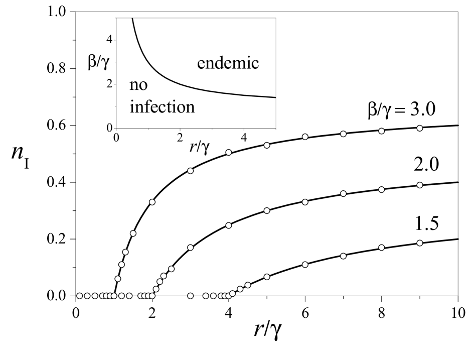
Figure 1: Long–time asymptotic fraction of infectious agents $n_{\rm I}$, as a function of the recombination rate $r$ (normalized by the recovery probability $\gamma$), for three values of the normalized infectivity $\beta/\gamma$. Curves and dots correspond, respectively, to analytical and numerical results. The inset shows, in the parameter plane ($r/\gamma,\beta/\gamma$), the boundary between the regimes of endemic infection and infection disappearance.

2.2 Evolution of the number of couples

Equivalent asymptotic results are obtained from mean field equations for the number of couples formed by agents with different epidemiological states. Note that, in our problem, the dynamics of the number of couples of different kinds corresponds to the evolution of links in the contact network. Let $m_{\rm SS}$, $m_{\rm IS}$, and $m_{\rm II}$ be the fraction of couples formed, respectively, by two S–agents, one I–agent and one S–agent, and two I–agents. Since at all times $m_{\rm SS}+m_{\rm IS}+m_{\rm II}=1$, it is enough to consider the evolution of only two of them, for instance, $m_{\rm SS}$ and $m_{\rm II}$. The mean field equations read

$$\begin{array}[]{ll}\dot{m}_{\rm SS}&=\frac{r}{4}m^{2}_{\rm IS}-rm_{\rm SS}m_{\rm II}+\gamma m_{\rm IS},\\ \dot{m}_{\rm II}&=\frac{r}{4}m^{2}_{\rm IS}-rm_{\rm SS}m_{\rm II}+\beta m_{\rm IS}-2\gamma m_{\rm II},\end{array}$$ (11)

with $m_{\rm IS}=1-m_{\rm SS}-m_{\rm II}$. The first two terms in the right–hand side of both equations stand for the only recombination events that change the number of couples of each kind, namely, (SS,II) $\leftrightarrow$ (IS,IS). The remaining terms correspond to the epidemiological events of contagion and recovery.

Equations (11) have two stationary solutions. One of them corresponds to the disappearance of the infection:

$$m_{\rm SS}=1,\ \ \ \ \ m_{\rm II}=0.$$ (12)

The other fixed point,

$$m_{\rm SS}=\frac{\gamma^{2}}{\beta^{2}r}(2\beta+2\gamma+r),\ \ \ \ \ m_{\rm II}=\frac{\beta-\gamma}{\beta^{2}r}[(\beta-\gamma)r-2\gamma^{2}],$$ (13)

corresponds to the endemic state. In agreement with the results of Section 2.1, the two stationary solutions interchange stability when the recombination rate attains the critical value given by Eq. (10). The infection level in the endemic state can be evaluated from the number of couples as $n_{\rm I}\equiv m_{\rm II}+m_{\rm IS}/2=(1+m_{\rm II}-m_{\rm SS})/2$ and coincides with the fraction of I–agents of Eq. (9).

3 Synchronization of coupled chaotic maps

The reappearance of the transition to endemic states in the monogamous SIS epidemiological model upon couple recombination events, opens the question of whether recombination may compensate disconnection for the occurrence of similar critical phenomena in other ensembles of interacting dynamical elements. In this section, we explore this question for the synchronization transition of coupled chaotic maps.

Consider an ensemble of $N$ identical chaotic maps whose individual states $x_{i}$ ($i=1,\dots,N$) evolve, in the absence of coupling, according to $x_{i}(t+1)=f[x_{i}(t)]$. Let $\lambda>1$ be the corresponding Lyapunov coefficient. On the average, the distance between two neighboring orbits of a map thus grows by a factor $\lambda$ at each iteration. Global (all-to-all) coupling between maps is introduced following the standard linear scheme [10, 11]

$$x_{i}(t+1)=(1-\varepsilon)f[x_{i}(t)]+\frac{\varepsilon}{N}\sum_{j=1}^{N}f[x_{j}(t)],$$ (14)

where $\varepsilon\in[0,1]$ is the coupling intensity. It is well known that, if coupling is strong enough, the ensemble undergoes a transition to full synchronization. Specifically, if

$$\varepsilon>\varepsilon_{c}=1-\frac{1}{\lambda},$$ (15)

coupling is able to overcome the exponential separation of chaotic orbits, and all the maps converge asymptotically to exactly the same trajectory: $x_{i}(t)=x_{j}(t)$ for all $i$, $j$ and $t\to\infty$ [11]. This synchronized trajectory is still chaotic –in fact, it reproduces the orbit of a single map– but the motion of the maps with respect to each other has been suppressed. Note that the threshold $\varepsilon_{c}$ for the synchronization transition does not depend on the ensemble size $N$.

Consider now a “monogamous” coupling pattern where, at any given time, each map is coupled to just one partner. Following the scheme of Eq. (14), if maps $a$ and $b$ form a couple, their states evolve according to

$$\begin{array}[]{ll}x_{a}(t+1)&=(1-\varepsilon)f[x_{a}(t)]+\frac{\varepsilon}{2}\left\{f[x_{a}(t)]+f[x_{b}(t)]\right\},\\ x_{b}(t+1)&=(1-\varepsilon)f[x_{b}(t)]+\frac{\varepsilon}{2}\left\{f[x_{a}(t)]+f[x_{b}(t)]\right\}.\end{array}$$ (16)

If $\varepsilon>\varepsilon_{c}$, the two maps will synchronize, converging asymptotically to the same chaotic orbit. Because of the nature of chaotic motion, however, their synchronized trajectory will differ from the orbits of other couples.

Would it be possible that, if couples of maps recombine exchanging partners at random at a certain rate, full synchronization all over the ensemble is recovered? By analogy with the occurrence of endemic states in SIS epidemics over a recombining monogamous population, we may expect that synchronization spreads over the ensemble if recombination is faster enough, entraining increasingly many maps towards the fully synchronized orbit. However, a difference with the case of SIS epidemic is that, now, the recombination rate has a limit: one random recombination per couple per iteration step produces the maximal possible rearrangement of the coupling pattern.

3.1 Synchronization dynamics within couples

To investigate whether full synchronization is possible in the monogamous coupling pattern under the effects of recombination, we assume that the ensemble is symmetrically concentrated around a reference orbit $x_{0}(t)$ of the map $f(x)$, so that the state of each map differs from $x_{0}(t)$ by a small amount: $x_{i}(t)=x_{0}(t)+\delta_{i}(t)$. If, as time elapses, the concentration around $x_{0}(t)$ grows in such a way that $\delta_{i}(t)\to 0$ for all $i$, full synchronization will be achieved. Equations (16) imply that the displacements of two coupled maps from the reference orbit $x_{0}(t)$ satisfy the linear equations

$$\begin{array}[]{ll}\delta_{a}(t+1)&=(1-\frac{\varepsilon}{2})f^{\prime}[x_{0}(t)]\delta_{a}(t)+\frac{\varepsilon}{2}f^{\prime}[x_{0}(t)]\delta_{b}(t),\\ \delta_{b}(t+1)&=(1-\frac{\varepsilon}{2})f^{\prime}[x_{0}(t)]\delta_{b}(t)+\frac{\varepsilon}{2}f^{\prime}[x_{0}(t)]\delta_{a}(t),\end{array}$$ (17)

where $f^{\prime}(x)$ is the derivative of $f(x)$.

Let us first study the simpler, extreme case where all couples recombine at each iteration step. Since new partners are chosen at random, the displacements $\delta_{a}(t)$ and $\delta_{b}(t)$ of the two coupled maps are uncorrelated quantities. In other words, the average $\zeta(t)=\langle\delta_{a}(t)\delta_{b}(t)\rangle$, performed over all the couples in the ensemble, vanishes. Consequently, from Eqs. (16), the variance of the displacement over the ensemble, $\sigma^{2}(t)=\langle\delta_{a}^{2}(t)\rangle$, is governed by

$$\sigma^{2}(t+1)=\left(1-\varepsilon+\frac{\varepsilon^{2}}{2}\right)f^{\prime}[x_{0}(t)]^{2}\sigma^{2}(t).$$ (18)

Taking into account that the long–time geometric mean value of $f^{\prime}[x_{0}(t)]^{2}$ is

$$\lim_{T\to\infty}\left(\prod_{t=t_{0}}^{t_{0}+T}f^{\prime}[x_{0}(t)]^{2}\right)^{1/T}=\lambda^{2},$$ (19)

the variance $\sigma^{2}$ will asymptotically vanish if $(1-\varepsilon+\varepsilon^{2}/2)\lambda^{2}<1$ or, equivalently, if

$$\varepsilon>\varepsilon_{1}=1-\frac{\sqrt{2-\lambda^{2}}}{\lambda}.$$ (20)

Thus, if the coupling intensity $\varepsilon$ is larger than the critical value $\varepsilon_{1}$, full synchronization is stable. Note that $\varepsilon_{1}>\varepsilon_{c}$ for any $\lambda\gtrsim 1$, so that full synchronization for maximal recombination rate requires stronger couplings than when the ensemble is globally coupled. Also, there is a critical limit $\lambda_{1}=\sqrt{2}\approx 1.41$ for the Lyapunov coefficient such that, if $\lambda>\lambda_{1}$, full synchronization is impossible even under the maximal recombination rate.

When recombination does not occur for all couples at all times, the joint evolution of two coupled maps introduces correlations between their displacements from the reference orbit. In this case, Eqs. (16) imply that $\zeta(t)=\langle\delta_{a}(t)\delta_{b}(t)\rangle$ and $\sigma^{2}(t)=\langle\delta_{a}^{2}(t)\rangle$ are governed by

$$\begin{array}[]{ll}\zeta(t+1)&=(1-\frac{\varepsilon}{2})\varepsilon f^{\prime}[x_{0}(t)]^{2}\sigma^{2}(t)+(1-\varepsilon+\frac{\varepsilon^{2}}{2})f^{\prime}[x_{0}(t)]^{2}\zeta(t),\\ \sigma^{2}(t+1)&=(1-\varepsilon+\frac{\varepsilon^{2}}{2})f^{\prime}[x_{0}(t)]^{2}\sigma^{2}(t)+(1-\frac{\varepsilon}{2})\varepsilon f^{\prime}[x_{0}(t)]^{2}\zeta(t).\end{array}$$ (21)

This linear system can be solved exactly. For the couples formed at a certain time $t_{0}$, we have $\zeta(t_{0})=0$ and $\sigma^{2}(t_{0})=\sigma_{0}^{2}$. With such initial conditions, and taking into account Eq. (19), the solution to Eqs. (21) for $\sigma^{2}$ reads

$$\sigma^{2}(t)=\frac{1}{2}\lambda^{2(t-t_{0})}\left[1+(1-\varepsilon)^{2(t-t_{0})}\right]\sigma_{0}^{2},$$ (22)

for $t\gg t_{0}$. This quantity is the variance of the displacement from $x_{0}(t)$ of those maps whose present couples have formed at time $t_{0}$ and lasted until the present time $t$.

Suppose now that, at a certain time $\tau$, the ensemble around $x_{0}(\tau)$ has variance $\sigma_{\tau}^{2}$. To evaluate the variance $\sigma_{\tau+1}^{2}$ at the next time step, we think of the ensemble as made up of subensembles consisting of the maps whose present couples have formed at times $\tau$, $\tau-1$, $\tau-2$, and so on. The fraction of maps in the subensemble corresponding to couples formed at time $\tau-n$ ($n=0,1,2,\dots$) is $q_{n}=r(1-r)^{n}$, where $r$ is the probability that any couple forms at any given time step ($0\leq r\leq 1$). Using Eq. (22) with $t\equiv\tau$ and $t_{0}\equiv\tau-n$, we find that the variance of this subensemble, which we denote $\sigma_{n}^{2}$, changes from $\sigma_{n}^{2}(\tau)=\sigma_{\tau}^{2}$ to

$$\sigma_{n}^{2}(\tau+1)=\lambda^{2}\frac{1+(1-\varepsilon)^{2(n+1)}}{1+(1-\varepsilon)^{2n}}\sigma_{\tau}^{2}.$$ (23)

Assuming that the ensemble has been evolving since an asymptotically long time ago, its variance at time $\tau+1$ is given by

$$\sigma_{\tau+1}^{2}=\sum_{n=0}^{\infty}q_{n}\sigma_{n}^{2}(\tau+1)=r\lambda^{2}\sum_{n=0}^{\infty}(1-r)^{n}\frac{1+(1-\varepsilon)^{2(n+1)}}{1+(1-\varepsilon)^{2n}}\sigma_{\tau}^{2}.$$ (24)

The synchronization threshold is therefore given by the condition

$$r\lambda^{2}\sum_{n=0}^{\infty}(1-r)^{n}\frac{1+(1-\varepsilon_{r})^{2(n+1)}}{1+(1-\varepsilon_{r})^{2n}}=1,$$ (25)

where $\varepsilon_{r}$ is the critical coupling intensity.

Note that, to obtain this result, we have used Eq. (22) for $t-t_{0}=n=0,1,2,\dots$ while, strictly, it holds for $t\gg t_{0}$ only. Consequently, the threshold condition (25) is just an approximation whose validity must be ascertained for each specific choice of the map $f(x)$. Below, we present numerical results for a case where Eq. (22) holds at any time.

Whereas, in general, the summation in Eq. (25) cannot be exactly performed, two special cases are readily obtained. The first one corresponds to the maximal recombination rate, $r=1$, for which we reobtain the critical coupling intensity $\varepsilon_{1}$ of Eq. (20). The second special case gives the recombination rate for which the threshold coupling intensity is maximal, $\varepsilon_{r}=1$, namely,

$$r_{\min}=2\left(1-\frac{1}{\lambda^{2}}\right).$$ (26)

For recombination rates below $r_{\min}$, synchronization is not possible even for the strongest coupling.

3.2 Numerical simulations

To test the above results we have performed numerical simulations of recombining monogamous ensembles of $N=10^{3}$ chaotic maps for the case of the tent map [9]:

$$f(x)=\left\{\begin{array}[]{ll}px&\mbox{for $0\leq x\leq\frac{1}{2}$},\\ p(1-x)&\mbox{for $\frac{1}{2}\leq x\leq 1$},\end{array}\right.$$ (27)

with $x\in[0,1]$ and $p\in[0,2]$. The Lyapunov coefficient of the tent map is $\lambda=p$, which implies that the dynamics is chaotic for $1<p\leq 2$. Moreover, $f^{\prime}(x)^{2}=p^{2}=\lambda^{2}$ for all $x$, so that in Eq. (19) the limit of $T\to\infty$ can be dropped, and Eq. (22) holds for any $t$.

In our simulations, after joint evolution of the coupled maps following Eq. (16), each one of the $N/2$ couples is allowed to recombine with probability $\rho$, exchanging partners with another randomly selected couple. Since two couples are involved at each recombination event, the resulting recombination probability per couple per time step is larger than $\rho$, and reads

$$r=1-(1-\rho)\exp(-\rho).$$ (28)

Fully synchronized ensembles are detected by numerically measuring the variance $\sigma_{x}^{2}(t)=N^{-1}\sum_{i}[x_{i}(t)-\bar{x}(t)]^{2}$ with respect to the average state $\bar{x}(t)=N^{-1}\sum_{i}x_{i}(t)$. Realizations where $\sigma_{x}^{2}(t)$ falls to the level of numerical round-off errors are identified with full synchronization.

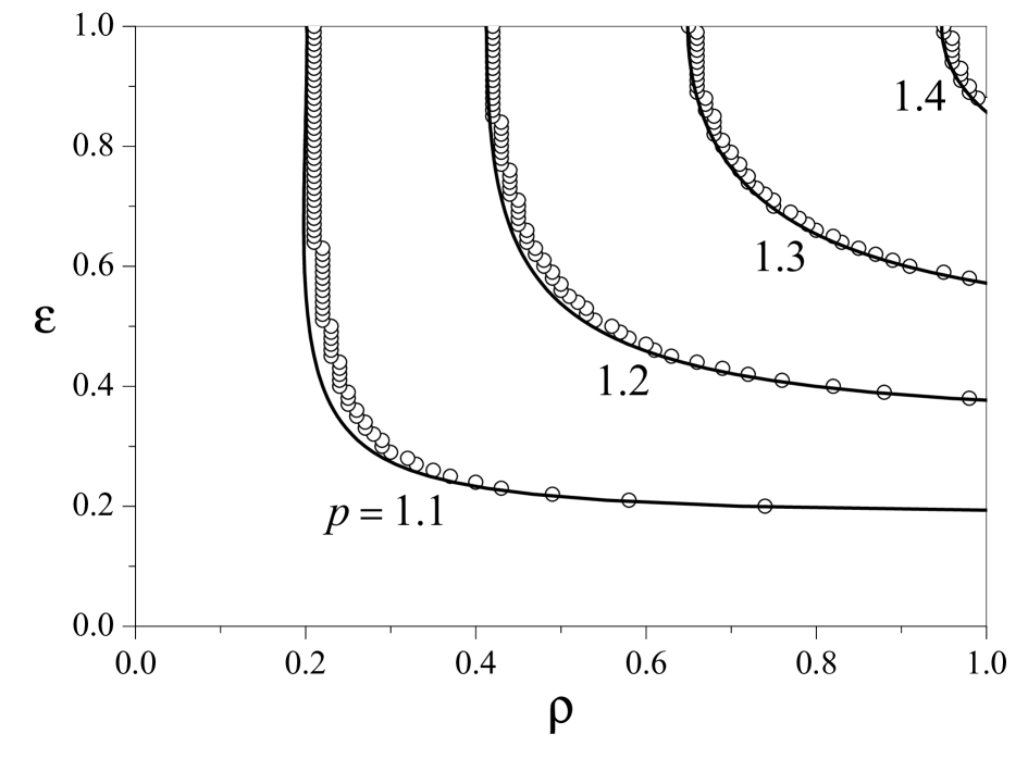
Figure 2: Full-synchronization threshold for a recombining monogamous ensemble of tent maps, in the parameter plane $(\rho,\varepsilon)$, for four values of the map parameter $p$. Full synchronization is stable above and to the right of each boundary. Dots and curves stand, respectively, for numerical results on ensembles of $10^{3}$ maps and the analytical result of Eq. (25). The numerical parameter $\rho$ is related to the recombination rate $r$ through Eq. (28).

Figure 2 shows the boundary of full synchronization in the parameter space $(\rho,\varepsilon)$ for four values of the tent map slope $p$. For each value of $\rho$, full synchronization is stable for coupling intensities $\varepsilon$ above the boundary. Dots stand for the numerical determination of the synchronization threshold and curves correspond to the analytical prediction, Eq. (25). The agreement is very good. The systematic difference between numerical and analytical results, more visible for small $p$, is to be ascribed to the numerical discretization of parameter space in the search for the synchronization threshold.

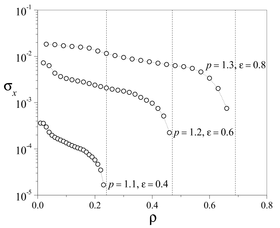
Figure 3: Dispersion of a recombining monogamous ensemble of $N=10^{3}$ tent maps as a function of the recombination parameter $\rho$, for three values of $p$ and $\varepsilon$. Vertical dashed lines stand for the numerical determination of the critical value of $\rho$, for each combination of $p$ and $\varepsilon$. Dotted curves are splines added as a guide to the eye.

In Fig. 3, we present numerical measurements of the long-time asymptotic values of the dispersion $\sigma_{x}$ as a function of $\rho$, for three combinations of $p$ and $\varepsilon$. Note that the drop of $\sigma_{x}$ at the critical recombination rate is abrupt but continuous.

3.3 Two-state symbolic dynamics

A description of the dynamics of the ensemble of coupled chaotic maps in terms of the evolution of different kinds of couple, along the lines developed in Section 2.2 for SIS epidemics, is in principle not possible. In fact, while the agents in the SIS population admit just two possible individual states –either susceptible or infectious, which determine three kinds of couple– the individual state of each chaotic map can span a continuous interval. However, as we show in this section, a symbolic representation of each map as a two-state variable –either synchronized or unsynchronized– together with a reduced set of transition rules between the two states, is able to qualitatively reproduce the collective effects of recombination on the synchronization transition. This schematic approach has the virtue of capturing the essential mechanisms of the interplay between recombination and synchronization, and can also be reinterpreted in the context of the SIS epidemics model.

Let us thus assume that, at any given time, each chaotic map adopts one of two states, namely, unsynchronized (U) or synchronized (S). We stress that synchronization of an individual map $i$ is here understood as defined with respect to the ensemble, for instance, if the variable $x_{i}(t)$ is within a certain small distance from the average $\bar{x}(t)=N^{-1}\sum_{j}x_{j}(t)$. In the spirit of Eqs. (11), we propose for the evolution of the fractions of couples $m_{\rm UU}$, $m_{\rm US}$, and $m_{\rm SS}$ the Ansatz

$$\begin{array}[]{ll}\dot{m}_{\rm UU}&=\frac{r}{4}m^{2}_{\rm US}-rm_{\rm SS}m_{\rm UU}+\gamma m_{\rm US}-\eta(r)m_{\rm UU},\\ \dot{m}_{\rm SS}&=\frac{r}{4}m^{2}_{\rm US}-rm_{\rm SS}m_{\rm UU}+\beta(r)m_{\rm US}+\eta(r)m_{\rm UU},\par\end{array}$$ (29)

with $m_{\rm US}=1-m_{\rm SS}-m_{\rm UU}$, and where $\beta(r)$, $\gamma$, and $\eta(r)$ are non–negative quantities. The first two terms in the right–hand side of both equations describe the effect of recombination at rate $r$ per couple. They have exactly the same origin as in Eqs. (11). The remaining terms, described in detail in the following, stand for the transitions induced by the joint evolution of coupled maps. Note that we are assuming that all these transitions occur always toward states where the two maps of a couple are either synchronized or unsynchronized. Also, we suppose that the two maps of an SS–couple, as long as their link lasts, cannot become unsynchronized from the ensemble.

In the first place, as time elapses, a US–couple can become either an SS–couple or a UU–couple. This describes the tendency towards synchronization within each couple. The rate for the transition US $\to$ SS, which we have called $\beta$ in Eqs. (29), cannot however be a constant. If it were a constant, in fact, all US–couples would become SS–couples for sufficiently long times, thus synchronizing with the ensemble even in the absence of recombination. This is not the case, though: when recombination is infrequent, maps forming a long-lasting couple synchronize to each other, but are generally not synchronized to the ensemble. We represent this effect phenomenologically, by ascribing to $\beta$ a dependence on $r$. The function $\beta(r)$ increases as $r$ grows, starting from $\beta(0)=0$.

The transition US $\to$ UU, on the other hand, implies the desynchronization of a map with respect to the ensemble by interaction with its already unsynchronized partner. This event does not require recombination: it is rather the generally expected outcome within a US couple. We thus assume that its rate, $\gamma$, is constant.

Finally, Eqs. (29) include, in the last terms of their right–hand side, the transition UU $\to$ SS. Because of the same reasons as in the case of the transition US $\to$ SS, which also involves the synchronization with the ensemble of previously unsynchronized maps, we expect that the corresponding rate, $\eta(r)$, is a growing function of the recombination rate $r$. Possibly, however, $\eta(r)$ is much smaller that $\gamma(r)$, because becoming an SS–couple should occur less frequently for a UU–couple than for a US–couple.

Equations (29) have two fixed points. One of them, $m_{\rm SS}=1$, $m_{\rm UU}=0$, corresponds to full synchronization of the ensemble of chaotic maps. For the other fixed point, both $m_{\rm SS}$ and $m_{\rm UU}$ are different from zero, thus corresponding to a state of partial synchronization. There is a broad choice of functional forms for $\beta(r)$ and $\eta(r)$ such that these stationary solutions have the expected behaviour –namely, that full synchronization is unstable for small $r$ and becomes stable above a critical value of the recombination rate, while the other fixed point exhibits opposite stability properties. For the sake of concreteness, let us assume the linear dependences $\beta(r)=\beta_{0}r$ and $\eta(r)=\eta_{0}r$. Analysis of the eigenvalues of Eqs. (29) around the fixed points shows that, irrespectively of the values of $\beta_{0}$ and $\gamma$, it is enough that $\eta_{0}<1$ for the occurrence of a transition to full synchronization as $r$ grows. The critical value of the recombination rate is

$$r_{c}=\frac{\gamma}{\beta_{0}}\frac{1-\eta_{0}}{1+\eta_{0}}.$$ (30)

Let us now attempt a semi–quantitative comparison of this result with our results for the synchronization transition in recombining monogamous ensembles of chaotic maps, for instance, those depicted in Fig. 2 for tent maps. Since $\gamma$ is the rate for the transition US $\to$ UU –where, by interaction within its couple, a map becomes desynchronized from the ensemble– it may be identified with a measure of the rate at which chaotic orbits diverge from each other, i.e. of the Lyapunov coefficient $\lambda$. The factor $\beta_{0}$, in turn, weights the rate of the transition US $\to$ SS, where a map becomes synchronized to the ensemble by interaction with its already synchronized partner. Thus, $\beta_{0}$ is related to the strength of the interaction between coupled maps, i.e. to the coupling intensity $\varepsilon$. The factor $\eta_{0}$ plays a similar role but, as mentioned above, its effect should be quantitatively less important than that of $\beta_{0}$. Figure 4 is a plot of the synchronization threshold as given by Eq. (30). To stress the correspondence with Fig. 2, we have plotted $\beta_{0}$ (a measure of the coupling intensity $\varepsilon$) as a function of the recombination rate $r$ (directly related, through Eq. (28), to the parameter $\rho$) for three values of $\gamma$ (a measure of the Lyapunov coefficient, $\lambda=p$ for the tent map), and fixed $\eta_{0}$. The semi–quantitative analogy with our numerical results for ensembles of tent maps, shown in Fig. 2, is apparent.

Figure 4: Synchronization threshold in the parameter plane ($r,\beta_{0}$) for the two–state model of coupled chaotic maps, corresponding to three values of the rate $\gamma$ and $\eta_{0}=0.01$. Full synchronization is stable in the region of large $r$ and $\beta_{0}$. Compare this plot with Fig. 2.

An analogy between this two–state approach to synchronization and the SIS epidemiological model discussed in Section 2 can in turn be derived from the identification of the unsynchronized state with the susceptible state on one hand, and of the synchronized state and the infectious state on the other. With this identification, the transitions US $\to$ SS and US $\to$ UU correspond, respectively, to contagion from the infectious partner and to the spontaneous recovery of an infectious agent. The rates $\beta$ and $\gamma$ play the same role in both dynamical models, with the difference that in the SIS model $\beta$ does not depend on the recombination rate. Another difference is that the two–state approach to synchronization includes the transition UU $\to$ SS, which in the SIS model would correspond to simultaneous infection of two susceptible partners –a forbidden event. The SIS model, in turn, allows for the recovery of just one among two infectious partners, which would stand for the inexistent transition SS $\to$ US. Notwithstanding these differences, we realize that the plot of Fig. 4 is the equivalent in the two–state approach to synchronization as the endemic threshold depicted in the insert of Fig. 1 –where both the infectivity $\beta$ and the recombination $r$ are normalized by the recovery probability $\gamma$. The two thresholds have qualitatively the same functional dependence on the respective parameter. In addition, the transition to full synchronization in our two–state formulation is a transcritical bifurcation, the same kind of critical phenomenon as in the SIS model.

4 Conclusion

We have here studied two critical phenomena in the collective behaviour of large ensembles of interacting dynamical elements –namely, the appearance of endemic states in an SIS epidemiological model, and the stabilization of full synchronization of identical chaotic maps– when the corresponding interaction patterns are highly disconnected and, concurrently, change with time. Specifically, we have considered “‘monogamous” interaction patterns, represented by networks where each site is connected to only one neighbour at a time, but such that neighbours can be exchanged at random at a specified rate. While in the absence of neighbour exchange –or, as we have called it, of recombination– the occurrence of endemic states and synchronization would be impossible due to the lack of connectivity in the ensemble, sufficiently frequent recombination events make it possible that coherence is established all over the system, thus allowing for organized collective dynamics.

Recombination of interacting couples in a monogamous pattern introduces a new dynamical parameter –the recombination rate. The two critical phenomena studied here take now place upon variation of this parameter: endemic states and full synchronization occur above a certain critical value of the recombination rate. Moreover, for the SIS epidemiological model with a given infectivity, we have found that the limit of infinitely large recombination rate is equivalent to the situation where the interaction pattern is static but not disconnected. For chaotic maps, on the other hand, the fact that time elapses by discrete steps imposes a limit to the recombination rate: any interacting couple can at most be recombined once per step. This establishes in turn an upper limit for the Lyapunov coefficient of individual maps such that they can be synchronized by recombination. If the maps are “too chaotic”, synchronization is not possible even at the maximal rate of one recombination per couple per time step.

The fact that, instantaneously, each dynamical element of the two ensembles considered here has just only one interaction partner, makes the corresponding problems analytically tractable to a large extent. In particular, we have obtained analytical approximations for the critical values of the recombination rate which are in very good agreement with numerical results. For SIS epidemics, the critical recombination rate was found both from the integration over the whole population of the epidemiological dynamics within each couple, and from the dynamics of the number of couples in each epidemiological state. For the chaotic maps, we have replaced this latter approach by a kind of symbolic schematic representation of the dynamics of couples. In this representation, which can also be adapted to the SIS model and qualitatively reproduces the critical behaviour of the two systems, maps (or epidemiological agents) are though of as two–state elements. Their interactions induce transitions between the two states following a small set of intuitive rules. We conjecture that this kind of representation is capturing the essential mechanisms that govern the relative prevalence of unsynchronized/susceptible elements at one side of the critical point, and of synchronized/infectious elements at the other.

Collective dynamics on monogamous interaction patterns have the advantage of analytical tractability. It should however be borne in mind that these patterns represent a kind of extreme case among disconnected networks: they have the minimal number of links that avoids isolated elements. Networks with less severe lack of connectivity should impose lower limitations to the development of collective self-organized behaviour. In these cases, therefore, we expect that recombination, even at lower rates, will also be able to compensate the lack of connectivity, triggering critical phenomena such as those studied here.

References

- [1] A. S. Mikhailov, Foundations of Synergetics I. Distributed Active Systems, 2nd edition (Springer, Heidelberg, 1994).
- [2] S. C. Manrubia, A. S. Mikhailov, and D. H. Zanette, Emergence of Dynamical Order: Synchronization Phenomena in Complex Systems (World Scientific, Singapore, 2004).
- [3] R. Pastor Satorras, J. Rubí and A. Díaz Guilera, eds., Statistical Mechanics of Complex Networks (Springer, Berlin, 2003).
- [4] K. T. D. Eames and M. J. Keeling, Math. Biosc. 189, 115 (2004).
- [5] M. J. Keeling and K. T. D. Eames, J. Royal Soc. Interface 2, 295 (2005).
- [6] E. Volz and L.A. Meyers, Proc. R. Soc. B 274, 2925 (2007).
- [7] S. Bouzat and D. H. Zanette, Eur. Phys. J. B 70, 557 (2009).
- [8] J. D. Murray, Mathematical Biology (Springer, Berlin, 1993).
- [9] S. H. Strogatz, Nonlinear Dynamics and Chaos (Westview, Cambridge, 2000).
- [10] K. Kaneko, Phys. Rev. Lett 63, 219 (1989).
- [11] K. Kaneko, Physica D 41, 137 (1990).