Renormalization and lattice artifacts

Chapter 0 Perturbative Renormalization

1 Introduction

Most of our present knowledge on the structure of renormalization of quantum field theories comes from perturbation theory (PT), a small coupling expansion around a free field theory. In this framework Feynman rules, derived formally in the continuum from the Gell-Mann–Low formula GellMann:1951rw or from the path integral approach, express amplitudes at a given order as sums of expressions associated with Feynman diagrams (see e.g. Nakanishi:1971). Tree diagrams are associated with well defined amplitudes, but for diagrams involving loops and associated integration over internal momenta one soon encounters divergent expressions e.g. for massive $g_{0}\phi^{4}$ theory in four euclidian dimensions the diagram in Fig. 1 is associated with the expression

$$I=g_{0}^{2}\int^{\Lambda}\mathrm{d}^{4}k\frac{1}{(k^{2}+m^{2})([(k+p)^{2}+m^{2}])}$$ (1)

which is logarithmically divergent as the ultra–violet (UV) cutoff $\Lambda\to\infty$. There are many ways to introduce an UV cutoff $\Lambda$ - a specification defines a particular regularization. The process of renormalization is then a well–defined prescription how to map regularized expressions to amplitudes which are finite when $\Lambda\to\infty$ while maintaining desired properties which are summarized by the Osterwalder–Schrader axioms (Osterwalder:1973dx, Osterwalder:1974tc) order by order in PT.

Figure 1: Simple 1–loop diagram

For lattice QCD renormalization is not needed if one is only interested in obtaining the low energy (LE) spectrum and scattering data. For such purposes we need knowledge of the phase diagram, the location of critical points where the continuum limit is reached, and the nature of the approach e.g. the question whether ratios of masses tend to their continuum limit as powers in the lattice spacing $a$:

$$\frac{m_{1}(a)}{m_{2}(a)}=\frac{m_{1}(0)}{m_{2}(0)}+C_{12}(am_{1})^{p}\,,\,\,\,p>0\,(?).$$ (2)

Lattice artifacts will be the topic of chapters 4–6. But perturbative and non-perturbative renormalization will be needed for 1) computing matrix elements of composite operators (describing probes of other interactions, finite temperature transport coefficients,….), 2) relating LE to high energy (HE) scales (e.g. computing running couplings and running masses), and 3) giving hints on the nature of lattice artifacts.

In this chapter we shall mainly consider perturbative renormalization; in chapter 2 we shall discuss renormalization group equations which follow from multiplicative renormalization, and aspects of non-perturbative renormalization will be the subject of chapter 3.

2 History and basic concepts

In a series of papers Reisz (Reisz:1987da–Reisz:1988kk) has proven perturbative renormalizability of lattice Yang–Mills theory and QCD (for a large class of actions). His proof is based mainly on methods developed with continuum regularization, (with some important modifications that we will mention later), so we will start the discussion with these.

Renormalization theory has a long and interesting history; here I reproduce a part of Wightman’s delightful discussion Wightman:1975gi since the reference is not always easily available.
“One of the first steps in natural history is to establish a classifactory nomenclature. I will do this for perturbative renormalization theory, but in so doing, I want to tell stories with a moral for an earnest student. Renormalization theory has a history of egregious errors by distinguished savants. It has a justified reputation for perversity; a method that works up to 13th order in the perturbation series fails in the 14th order. Arguments that sound plausible often dissolve into mush when examined closely. The worst that can happen often happens. The prudent student would do well to distinguish sharply between what has been proved and what has been made plausible, and in general he should watch out!

Figure 2: Troublesome $14$’th oder QED diagram

My first cautionary tale has to do with the early days of renormalization theory. When F.J. Dyson analyzed the renormalization theory of the S–matrix for quantum electrodynamics of spin one-half particles in his two great papers of 1948–9, (Dyson:1949bp, Dyson:1949ha) he laid the foundations for most later work on the subject, but his treatment of one phenomenon, overlapping divergences was incomplete. Among the methods offered to clarify the situation, that of J. Ward Ward:1951 seemed outstandingly simple, so much so that it was adopted in Jauch and Rohrlich’s standard text book Jauch:1955. Several years later Mills and Yang noticed that unless further refinements are introduced the method does not work for the photon self energy Wu:1962zza. The lowest order for which the trouble manifests itself is the fourteenth e.g. in the (7–loop) graph Fig. 2. Mills and Yang repaired the method and sketched some of the steps in a proof that it would yield a finite renormalized amplitude Mills:1966vn. An innocent reading of the textbook of Jauch and Rohrlich, would never suspect such refinements are necessary.

Another attempt to cope with the overlapping divergences was made by Salam (Salam:1951sm, Salam:1951sj). I will not describe it, if for no other reason than that I never have succeeded in understanding it. Salam and Matthews commenting on this and related work somewhat later Matthews:1951sk remarked “… The difficulty, as in all this work is to find a notation which is both concise and intelligible to at least two people of whom one may be the author”. The belief is widespread that when Salam’s work is combined with later significant work by S. Weinberg Weinberg:1959nj, the result should be a mathematically consistent version of renormalization theory. At least that is what one reads in the text book of Bjorken and Drell for quantum electrodynamics Bjorken:1965, and in the work of R. Johnson Johnson:1970it and the lectures of K. Symanzik for meson theories Symanzik:1961. So apparently the Matthews–Salam criterion has been satisfied. I only wish they had spelled it out a little for the peasants.

Another foundation of renormalization theory with a rather different starting point was put forward by Stueckelberg and Green Stueckelberg:1951. It was refounded and brought to a certain stage of completion in the standard text book of Bogoliubov and Shirkov Bogoliubov:1959. The mathematical nut that had to be cracked is in the paper of Bogoliubov and Parasiuk Bogoliubov:1957gp, (amazingly, not quoted in the English translation of Bogoliubov and Shirkov) . This paper introduces a systematic combinatorial and analytic scheme for overcoming the overlapping divergence problem. This paper is very important for later developments. Unfortunately it was found by K. Hepp Hepp:1966eg that Theorem 4 of the paper is false, and that consequently the proof of the main result is incomplete as it stands. However Hepp found that Theorem 4 is not essential to derive the main result and he could fill all the gaps. Thus it is appropriate to introduce the initials BPH to stand for the renormalization method described in Bogoliubov:1957gp and Hepp:1966eg. So far as I know it was the first version of renormalization theory on a mathematically sound basis.”

The rest of the article is also highly recommendable. Reading his article one can understand why many workers in the field who had gone through these historical developments were wary about renormalization theory . A real breakthrough in the ease of understanding was supplied by Zimmermann (Zimmermann:1968mu, Zimmermann:1972te, Zimmermann:1972tv), (in particular also concerning renormalization of composite operators). I strongly recommend Lowenstein’s article Lowenstein:1975ug for a clear exposition of Zimmermann’s methods.

It is the purpose of this chapter to give an overview of the important steps and concepts of perturbative renormalization, stating the main results without proofs; for the latter the interested reader must consult further literature. Moreover I will only discuss the standard approach using expansions in Feynman diagrams, but I would like to mention a powerful alternative approach using flow equations based on the renormalization group developed by Wilson (Wilson:1971bg, Wilson:1971dh, Wilson:1973jj) and improved by Polchinski Polchinski:1983gv, a framework which is well suited for proving structural results, see e.g. the works of Keller, Kopper and Salmhofer Keller:1990ej, Salmhofer:1999uq.

3 Perturbative classification of theories

Concerning the nature of a Feynman diagram the first important concept is its superficial degree of divergence. Consider a diagram with $E$ external lines, $V$ internal vertices, $P$ internal lines and $\ell$ independent loops. There are some relations between these the first of which is the topological relation

$$V+\ell-P=\mathrm{number\,\,of\,\,connected\,\,components}\,.$$ (3)

Other relations depend on the precise nature of the vertices in the theory e.g. with only a 4–point vertex:

$$4V=2P+E\,.$$ (4)

Then for a connected diagram $\Gamma$ with $\ell$ loops the superficial degree of divergence $\delta(\Gamma)$ estimates the behavior of the associated integral when all internal momenta are large. For $\phi^{4}_{d}$ theory (in $d$ space–time dimensions):

$$\delta(\Gamma) = d\ell-2P$$ (5)

$$= d-\frac{1}{2}(d-2)E+(d-4)V\,.$$ (6)

For $d=4$ this simplifies to $\delta(\Gamma)=4-E\,,$ which is negative for $E>4$ indicating possible overall convergence of the integral in this case.

Exercise 3.1.

Show $\delta(\Gamma)=6-2E$ for $\phi^{3}_{6}$ theory.

This theory is often discussed in the literature because of the comparative simplicity of the diagrams involved. In this case $\delta(\Gamma)$ is negative for $E>3$.

Figure 3: 2–loop diagram in $\phi^{3}_{6}$ theory with a nested divergence

It is clear that considerations of $\delta(\Gamma)$ alone are not sufficient to establish convergence of the integral because $\Gamma$ could have divergent sub-diagrams as in Fig. 3. However it does lead to the following classification of perturbative QFT:

• super–renormalizable: theories where only a finite number of diagrams have $\delta\geq 0$.

• renormalizable: there exists $E_{0}<\infty$ such that all diagrams with $E>E_{0}$ have $\delta<0$.

• non–renormalizable: all $E$–point diagrams have $\delta\geq 0$ for sufficiently high number of loops $\ell$.

Remarks: i). Non-renormalizable theories are not necessarily unphysical or devoid of predictive power (an interesting example concerns gravity Donoghue:1995cz). They can be good effective theories, such as chiral Langrangians discussed in Goltermann’s lectures.

ii) Non–perturbative formulations of perturbatively renormalizable theories may be trivial in the limit that the ultra–violet cutoff is sent to infinity . Examples of such theories are thought to be $\phi^{4}$ and QED in 4–dimensions, albeit there is at present no rigorous proof of this conventional wisdom.

iii) There are some rigorous non-perturbative constructions of super–renormalizable theories e.g. $\phi^{4}_{2}$ Glimm:1968kh, Yukawa theory in 2–dimensions Seiler:1975gs, $\phi^{4}_{3}$ Feldman:1975da. The Schwinger functions in the topologically trivial sector of SU(2) Yang–Mills theory in 4–dimensions in a sufficiently small volume have also been rigorously constructed (Magnen:1992ww, Magnen:1992wv). For all of these cases the structural information on renormalization found in perturbation theory carry over to the non–perturbative framework.

In the following we restrict attention to renormalizable theories. A generic procedure to put perturbative renormalization on a firm mathematical basis consists of three steps:

1. Introduce an UV regularization.

2. Construct a mapping of a Feynman integral to an absolutely convergent integral when the cutoff is removed.

3. Show that the map in step 2 is equivalent to a renormalization of the bare parameters and fields in the original Lagrangian, which formally ensures the desired axiomatic properties of the resulting amplitudes.

There are many perturbative regularization procedures , each with their own advantages and disadvantages. In all cases known they give equivalent physical results.

4 Zimmermann’s forest formula

Let us first restrict attention to theories with massive bare propagators. Returning to the simple 1–loop example (1), the integral can obviously be made convergent if the integrand is subtracted at external momentum $p=0$:

$$I\rightarrow R=g_{0}^{2}\int^{\Lambda}\mathrm{d}^{4}k\left[\frac{1}{(k^{2}+m^{2})([(k+p)^{2}+m^{2})}-\frac{1}{(k^{2}+m^{2})^{2}}\right]\,.$$ (7)

We note that since the subtraction is a constant (independent of the external momenta) it can be absorbed in a renormalization of the bare coupling $g_{0}$.

The problem now is to find the generalization of the subtraction in the simple case above for an arbitrary diagram. For this purpose we can restrict attention to one particle irreducible (1PI) diagrams, diagrams which remain connected after cutting any internal line, since an arbitrary diagram can be constructed from 1PI parts joined by propagators.

Figure 4: 2–loop diagram with overlapping divergences

Here we consider mappings where subtractions are made directly on the integrands, as adopted by Reisz for the lattice regularization . Let $I_{\Gamma}(p,k)$ be the original integrand of a diagram with external momenta $p=\{p_{1},p_{2},\dots\}$ and internal momenta $k=\{k_{1},k_{2},\dots\}$. The regularized integral will then be given by

$$R_{\Gamma}(p)=\int\prod_{j}\mathrm{d}^{d}k_{j}\,R_{\Gamma}(p,k)\,,$$ (8)

with

$$R_{\Gamma}(p,k) = I_{\Gamma}(p,k)-\mathrm{subtractions}$$ (9)

$$= \left(1-t_{p}^{\delta(\Gamma)}\right)\overline{R}_{\Gamma}(p,k)\,,$$ (10)

where $t_{p}^{\delta}$ is the Taylor operator of degree $\delta$:

$$t_{p}^{\delta}F(p)=F(0)+p_{i}^{\mu}\frac{\partial}{\partial p_{i}^{\prime\mu}}F(p^{\prime})|_{p^{\prime}=0}+\dots+\frac{1}{\delta!}p_{i_{1}}^{\mu_{1}}\dots p_{i_{\delta}}^{\mu_{\delta}}\frac{\partial}{\partial p_{i_{1}}^{\prime\mu_{1}}}\dots\frac{\partial}{\partial p_{i_{\delta}}^{\prime\mu_{\delta}}}F(p^{\prime})|_{p^{\prime}=0}\,.$$ (11)

Dyson’s original proposal Dyson:1949ha was

$$\overline{R}_{\Gamma}(p,k)=\prod_{\gamma,1PI\subset\Gamma}\left(1-t_{p^{\gamma}}^{\delta(\gamma)}\right)I_{\Gamma}(p,k)$$

where $p^{\gamma}$ are the external momenta of $\gamma$. On the rhs of this equation the term involving $\gamma_{1}$ is to the right of that for $\gamma_{2}$ if $\gamma_{1}$ is nested in $\gamma_{2}$ i.e. $\gamma_{1}\subset\gamma_{2}$. If sets of lines of $\gamma_{1}$ and $\gamma_{2}$ do not intersect then the order is irrelevant. The proposal cures the problem of nested divergences, however no prescription is given how to order overlapping divergences, that is divergent sub-diagrams which have non-trivial intersection but are not nested such as in Fig. 4 .

The correct prescription presented by Zimmermann Zimmermann:1968mu is obtained by expanding Dyson’s product and dropping all terms containing products of terms involving overlapping sub-diagrams. The result is called Zimmermann’s forest formula:

$$\overline{R}_{\Gamma}(p,k)=\sum_{\mathcal{F}}\prod_{\gamma\in\mathcal{F}}\left(-t_{p^{\gamma}}^{\delta(\gamma)}\right)I_{\Gamma}(p,k)$$ (12)

where the sum is over all forests:

$$\mathcal{F} = \{\gamma|\gamma{\rm\,\,1PI\,,\,}\delta(\gamma)\geq 0;$$

$$\gamma_{1},\gamma_{2}\in\mathcal{F}\Rightarrow\gamma_{1}\subset\gamma_{2}\,\,\mathrm{or}\,\,\gamma_{2}\subset\gamma_{1}\,\,\mathrm{or}\,\,\gamma_{1},\gamma_{2}\,\,\mathrm{non-overlapping}\}\,.$$

The empty set $\phi$ is included as a special forest.

Exercise 4.1.

Give the set of forests for the diagram in Fig. 5 (it has 8 elements).

The following rules are used to specify the momenta flow in $\Gamma$ and its subgraphs. The momenta flowing in the $\sigma$’th internal line $L_{ab\sigma}$ joining vertices $a,b$ is specified as $l_{ab\sigma}=P_{ab\sigma}(p)+K_{ab\sigma}(k)$ with $K_{ab\sigma}=\sum_{i}\epsilon_{ab\sigma i}k_{i}$; $\epsilon_{ab\sigma i}=1$ if $l_{ab\sigma}\in$ loop ${\mathcal{C}}_{i}$; $\epsilon_{ab\sigma i}=-1$ if $l_{ba\sigma}\in$ loop ${\mathcal{C}}_{i}$; $\epsilon_{ab\sigma i}=0$ otherwise. The momentum $P_{ab\sigma}$ is solved by Kirchoff’s laws: $\sum_{b\sigma}P_{ab\sigma}+p_{a}=0$. $\sum_{L_{ab\sigma}\in{\mathcal{C}}_{i}}r_{ab\sigma}P_{ab\sigma}=0$. Here “resistances” $r_{ab\sigma}$ can be chosen for convenience (including zero) but no closed loop of zero resistances.

Similarly for subdiagrams $\gamma$: $l^{\gamma}_{ab\sigma}=P^{\gamma}_{ab\sigma}(p^{\gamma})+K^{\gamma}_{ab\sigma}(k)$. First solve for $P^{\gamma}_{ab\sigma}$ keeping same resistances and momentum conservation at the vertex. Then determine the $K^{\gamma}_{ab\sigma}(k)$ from $l^{\gamma}_{ab\sigma}=l_{ab\sigma}$.

Figure 5: 3–loop diagram in $\phi^{3}_{3}$ theory

After applying the forest formula the resulting integrand has a form

$$F(p,k)=\frac{V(k,p,m)}{\prod_{i=1}^{n}\left(l_{i}^{2}+m^{2}\right)}\,,$$ (13)

where

$$l_{i}=K_{i}(k)+P_{i}(p)\,.$$ (14)

To proceed it is first necessary to give conditions on such an integrand required to guarantee the convergence of the corresponding integral

$$F(p)=\int\mathrm{d}^{d}k_{1}\dots\mathrm{d}^{d}k_{\ell}\,F(p,k)\,.$$ (15)

Here and in the following we will assume that the internal momenta have been selected in a “natural way” so that $K_{i}=k_{i}$ for $i=1,\dots,\ell$ (this is always possible). Consider the set

$$\mathcal{L}=\{K_{1},\dots,K_{n}\}\,,$$ (16)

and let $u_{1},\dots,u_{r},v_{1},\dots,v_{\ell-r}\,\,\,r\geq 1\,,$ be $\ell$ linearly independent elements of $\mathcal{L}$. Let $H$ be the (Zimmermann) subspace spanned by the $u_{i}$. Then the upper degree of a function $f(u,v)$ with respect to $H$ is given by

$$\overline{\mathrm{deg}}_{u|v}f(u,v)=\overline{\nu}\,\,\,\,\,\mathrm{if}\,\,\,\,\,\lim_{\lambda\to\infty}\lambda^{-\overline{\nu}}f(\lambda u,v)\neq 0,\infty\,,$$ (17)

and for the integral (15) the upper degree wrt $H$ is defined by

$$\overline{\mathrm{deg}}_{H}F(p)=dr+\overline{\mathrm{deg}}_{u|v}F(p,k(u,v,p))\,.$$ (18)

The important statement is Dyson’s power counting theorem: $F(p)$ in (15) is absolutely convergent if $\overline{\mathrm{deg}}_{H}F(p)<0$ for all subspaces $H$.

The theorem was first proven by Weinberg Weinberg:1959nj, and later a simpler proof was given by Hahn and Zimmermann Hahn:1968.

It can be shown that the forest formula yields integrals $F(p)=R_{\Gamma}(p)$ whose integrands satisfy the conditions of the theorem. Once this is done it remains to prove step 3 of the renormalization procedure (see sect. 1.3). This is not at all obvious from the forest formula as it stands. For this purpose it is advantageous to show that the forest formula is a solution to the Bogoliubov–Parasiuk–Hepp recursion relations (Bogoliubov:1959, Bogoliubov:1957gp, Hepp:1966eg) :

$$\overline{R}_{\Gamma}=\sum_{\psi}\prod_{\gamma\in\psi}(-t^{\delta(\gamma)})\overline{R}_{\gamma}\,,$$ (19)

where $\psi$ are sets of disjoint 1PI subgraphs. This formula serves as a basis for an inductive proof of step 3; again the proof is too long to present here ; a tactic to prove multiplicative renormalizability of gauge theories will be given in sect. 1.6.

5 Renormalization of theories with massless propagators

For theories with massless bare propagators one must control possible infra-red (IR) divergences. To this end for a Zimmermann subspace one defines a lower degree:

$$\underline{\mathrm{deg}}_{v|u}f(u,v)=\underline{\nu}\,\,\,\,\,\mathrm{if}\,\,\,\,\,\lim_{\lambda\to 0}\lambda^{-\underline{\nu}}f(\lambda u,v)\neq 0,\infty\,,$$ (20)

and for the integral (15):

$$\underline{\mathrm{deg}}_{H^{\prime}}F(p)=d(\ell-r)+\underline{\mathrm{deg}}_{v|u}F(p,k(u,v,p))\,.$$ (21)

The appropriately modified power counting theorem then states that $F(p)$ is absolutely convergent if $\overline{\mathrm{deg}}_{H}F(p)<0$ and $\underline{\mathrm{deg}}_{H^{\prime}}F(p)>0$ for all $H$ and for all non–exceptional external momenta $p$ (that is a set for which no partial sum of external momenta vanish, except for the complete sum expressing total momentum conservation).

To achieve this one has to modify the $R$–operation described above to avoid IR divergences introduced by Taylor subtractions at $p=0$. One way, introduced by Lowenstein and Zimmermann Lowenstein:1975rg and adopted by Reisz (Reisz:1987pw, Reisz:1987hx) is to introduce an auxiliary mass in the massless propagators $l^{2}\to l^{2}+(1-s)\mu^{2}$. UV subtractions are then made at $p=0,s=0$, and afterwards $s$ is set to 1 in the remaining parts. In order to avoid further IR singularities it is usually necessary to make extra finite subtractions to ensure 2– and 3–point functions vanish at exceptional external momenta singularities. In gauge theories this is guaranteed by the Slavnov–Taylor identities which we consider in the next section.

6 Renormalization of 4-d Yang–Mills theory

In this section we will outline the proof of multiplicative renormalizability of Yang–Mills (YM) theory in 4 dimensions. Perturbation theory is an expansion around a saddle point. For gauge theories, such as pure YM theory, gauge invariance of the action implies severe degeneracy of the saddle point. To apply perturbation theory one needs to lift the degeneracy by gauge fixing (see Lüscher’s elegant discussion Luscher:1988sd) . It is convenient to employ linear gauge fixing functions, e.g. the Lorentz gauge, which transform under the adjoint representation of the global gauge group so that the gauge fixed action is invariant under such transformations. Because of the non-linearity of the YM theory this way of fixing the gauge introduces extra terms in the functional integral, which can be expressed as a local Lagrangian involving Faddeev-Popov ghost fields $c,\bar{c}$ as introduced in Hernandez’ lectures. The action in this case is

$$S_{0} = -2\int\mathrm{tr}\left\{\frac{1}{4}F^{2}+\frac{\lambda_{0}}{2}(\partial A)^{2}-\bar{c}\partial_{\mu}\left[D_{\mu},c\right]\right\}$$ (22)

$$= S_{A}+S_{\mathrm{gf}}+S_{\mathrm{FP}}\,,$$ (23)

where $D_{\mu}=\partial_{\mu}+g_{0}A_{\mu}$ and $F_{\mu\nu}=\partial_{\mu}A_{\nu}-\partial_{\nu}A_{\mu}+g_{0}\left[A_{\mu},A_{\nu}\right]\,.$ Here $A_{\mu}=T_{d}A_{\mu}^{d}$ where $T_{d}$ denote a basis of the Lie algebra of SU($N$) with $\mathrm{tr}(T_{d}T_{e})=-\frac{1}{2}\delta_{de}$.

The action is no longer gauge invariant but an important property is that $S_{A}$ and $S_{\mathrm{gf}}+S_{\mathrm{FP}}$ are separately invariant under BRST transformations Becchi:1975nq:

$$\delta A_{\mu} = \epsilon sA_{\mu}=\epsilon\left[D_{\mu},c\right]\,,$$ (24)

$$\delta c = \epsilon sc=-\epsilon g_{0}c^{2}\,,$$ (25)

$$\delta\overline{c} = \epsilon s\overline{c}=\epsilon\lambda_{0}\partial_{\mu}A_{\mu}\,,$$ (26)

where $\epsilon$ is an infinitesimal Grassmann parameter.

Exercise 6.1.

Show the BRST invariance of $S_{\mathrm{gf}}+S_{\mathrm{FP}}$.

Note that $s$ is nilpotent: $s^{2}H[A,\bar{c},c]=0$ for all functionals $H$. This property and the BRST invariance of the action and measure imply the powerful Slavnov–Taylor identities Slavnov:1972fg, Taylor:1971ff ; for any functional $H[A,\bar{c},c]$:

$$\langle sH\rangle=0\,.$$ (27)

For example if we take $H=\bar{c}^{a}(x)\partial_{\nu}A_{\nu}^{b}(y)$ we obtain

$$\langle\lambda_{0}\partial_{\mu}A_{\mu}^{a}(x)\partial_{\nu}A_{\nu}^{b}(y)\rangle = \langle\bar{c}^{a}(x)\partial_{\nu}\left[D_{\nu},c\right]^{b}(y)\rangle$$ (28)

$$= \delta^{ab}\delta(x-y)\,,$$ (29)

where in the last line the ghost field equation of motion has been used. It follows that the full (bare) gluon propagator has the form

$$\widetilde{D^{\prime}}^{ab}_{\mu\nu}(k)=\frac{\delta_{ab}}{k^{2}}\left[\frac{\delta_{\mu\nu}-k_{\mu}k_{\nu}/k^{2}}{1+\Pi(k^{2})}+\frac{1}{\lambda_{0}}\frac{k_{\mu}k_{\nu}}{k^{2}}\right]\,.$$ (30)

More generally BRST invariance gives relations between bare Green functions and those containing composite operator insertions which describe the non-linear symmetry transformations of the fields. Many features of the theory derive from these Ward identities. In particular they are sufficient to restrict the structure of the counter-terms and show multiplicative renormalizability i.e. the theory is renormalized by adjusting the bare parameters and fields of the bare action. Also the renormalized theory satisfies similar symmetry properties as the bare one , which is also crucial to prove the IR finiteness of correlation functions with non-exceptional kinematics.

To proceed systematically the WI’s are summarized in equations for generating functionals Becchi:1975nq, ZinnJustin:2002ru such as

$$Z_{0}(J,\bar{\xi},\xi,K,L;g_{0},\lambda_{0}) = N_{0}\int D[A]D[c]D[\bar{c}]\exp\Bigl{\{}{\mathcal{E}}_{0}(A,c,\bar{c},K,L;g_{0},\lambda_{0})$$ (31)

$$+ \frac{1}{\hbar}S_{c}(A,c,\bar{c};J,\bar{\xi},\xi)\Bigr{\}}\,,$$

where $N_{0}$ is chosen such that $Z_{0}(\mathrm{all\,\,sources}\,=0;g_{0},\lambda_{0})=1$. The term $S_{c}$ contains source terms for the basic fields

$$S_{c}(A,c,\bar{c};J,\bar{\xi},\xi)=\int_{x}\sum_{b}\left\{J_{\mu}^{b}(x)A^{b}_{\mu}(x)+\bar{\xi}^{b}(x)c_{b}(x)+\bar{c}^{b}(x)\xi_{b}(x)\right\}\,,$$ (32)

and

$${\mathcal{E}}_{0}(A,c,\bar{c},K,L;g_{0},\lambda_{0}) = \frac{1}{\hbar}\int_{x}\sum_{b}\left\{K^{b}_{\mu}(x)sA_{\mu}^{b}(x)+L^{b}(x)sc^{b}(x)\right\}$$ (33)

$$-\frac{1}{\hbar}S_{0}(A,c,\bar{c};g_{0},\lambda_{0})\,,$$

where the new sources $K,L$ must be introduced for the composite fields appearing in the BRS transformations. Note that since $s$ is nilpotent further sources in $Z_{0}$ are not needed. The factors of $\hbar$ in diagrammatic contributions to correlation functions count the number of associated loops.

Now the BRS transformations imply that $Z_{0}$ satisfies

$$\int_{x}\sum_{b}\left\{J_{\mu}^{b}(x)\frac{\partial}{\partial K_{\mu}^{b}(x)}-\bar{\xi}_{b}\frac{\partial}{\partial L^{b}(x)}-\lambda_{0}\xi^{b}(x)\partial_{\mu}\frac{\partial}{\partial J^{b}_{\mu}(x)}\right\}Z_{0}=0\,,$$ (34)

and the same equation holds for the generating functional of the connected Green functions $W_{0}=\hbar\ln Z_{0}$. For considerations of renormalizability we have already noted that it is more convenient to consider 1PI diagrams. The generating functional $\Gamma_{0}$ for these is called the vertex functional (see Hernandez’ lectures) which is obtained from $W_{0}$ via a Legendre transformation,

$$W_{0}(J,\bar{\xi},\xi,K,L;g_{0},\lambda_{0})=\Gamma_{0}(A,c,\bar{c},K,L;g_{0},\lambda_{0})$$ (35)

$$+ \int_{x}\left\{J^{b}_{\mu}(x)A^{b}_{\mu}(x)+\bar{\xi}^{b}(x)c^{b}(x)+\bar{c}^{b}(x)\xi^{b}(x)\right\}\,,$$

where

$$A_{\mu}^{b}(x)=\frac{\partial W_{0}}{\partial J_{\mu}^{b}(x)}\,,\,\,\,c^{b}(x)=\frac{\partial W_{0}}{\partial\bar{\xi}^{b}(x)}\,,\,\,\,\bar{c}^{b}(x)=-\frac{\partial W_{0}}{\partial\xi^{b}(x)}\,,\,\,\,$$ (36)

with inverse relations

$$J_{\mu}^{b}(x)=-\frac{\partial\Gamma_{0}}{\partial A_{\mu}^{b}(x)}\,,\,\,\,\bar{\xi}^{b}(x)=\frac{\partial\Gamma_{0}}{\partial c^{b}(x)}\,,\,\,\,\xi^{b}(x)=-\frac{\partial\Gamma_{0}}{\partial\bar{c}^{b}(x)}\,.$$ (37)

The vertex functional satisfies the equation

$$\int_{x}\left\{\frac{\partial\Gamma_{0}}{\partial A_{\mu}^{b}(x)}\frac{\partial\Gamma_{0}}{\partial K_{\mu}^{b}(x)}+\frac{\partial\Gamma_{0}}{\partial c^{b}(x)}\frac{\partial\Gamma_{0}}{\partial L^{b}(x)}-\lambda_{0}\partial_{\mu}A^{b}_{\mu}(x))\frac{\partial\Gamma_{0}}{\partial\bar{c}^{b}(x)}\right\}=0\,.$$ (38)

Setting

$$\overline{\Gamma}_{0}=\Gamma_{0}+\int_{x}(\lambda_{0}/2)\left(\partial_{\mu}A^{b}_{\mu}(x)\right)^{2}\,,$$ (39)

and using the FP ghost field equation

$$\partial_{\mu}\frac{\partial\overline{\Gamma}_{0}}{\partial K^{b}_{\mu}(x)}+\frac{\partial\overline{\Gamma}_{0}}{\partial\bar{c}^{b}(x)}=0\,,$$ (40)

we can write the WI in a slightly simpler form

$$\int_{x}\left\{\frac{\partial\overline{\Gamma}_{0}}{\partial A_{\mu}^{b}(x)}\frac{\partial\overline{\Gamma_{0}}}{\partial K_{\mu}^{b}(x)}+\frac{\partial\overline{\Gamma}_{0}}{\partial c^{b}(x)}\frac{\partial\overline{\Gamma}_{0}}{\partial L^{b}(x)}\right\}=0\,.$$ (41)

We now seek a functional ${\mathcal{E}}_{\mathrm{R}}={\mathcal{E}}_{0}+\mathrm{O}(\hbar)$ such that Green functions generated from

$$Z_{\mathrm{R}}(J,\bar{\xi},\xi,K,L;g_{0},\lambda_{0}) = N_{\mathrm{R}}\int D[A]D[c]D[\bar{c}]\exp\Bigl{\{}{\mathcal{E}}_{\mathrm{R}}(A,c,\bar{c},K,L;g,\lambda)$$ (42)

$$+(1/\hbar)S_{c}(A,c,\bar{c};J,\bar{\xi},\xi)\Bigr{\}}$$

are finite order by order in PT . Such a functional can be found and is simply characterized by the following
Renormalization Theorem: There exist renormalization constants $Z_{1},Z_{3},\widetilde{Z}_{3}$ which are formal power series in $\hbar$, relating bare fields and renormalized fields

$$A^{0} = Z_{3}^{1/2}A\,,\,\,L^{0}=Z_{3}^{1/2}L\,,\,\,\,\lambda_{0}=Z_{3}^{-1}\lambda\,,\,\,g_{0}=Z_{1}g\,,$$ (43)

$$c^{0} = \widetilde{Z}_{3}^{1/2}c\,,\,\,\bar{c}^{0}=\widetilde{Z}_{3}^{1/2}\bar{c}\,,\,\,K^{0}=\widetilde{Z}_{3}^{1/2}K\,,$$ (44)

such that

$${\mathcal{E}}_{\mathrm{R}}(A,c,\bar{c},K,L;g_{0},\lambda_{0})={\mathcal{E}}_{0}(A^{0},c^{0},\bar{c}^{0},K^{0},L^{0};g_{0},\lambda_{0})\,.$$ (45)

Furthermore the $Z$’s have only (multi-) poles in $\epsilon$ with dimensional regularization (DR) ’tHooft:1972fi, (Breitenlohner:1975hg, Breitenlohner:1976te), Collins:1984xc, or depend only logarithmically on a momentum cutoff with other regularizations.

The renormalization theorem implies $\overline{\Gamma}_{\mathrm{R}}(A,c,\bar{c},K,L;g,\lambda)=\overline{\Gamma}_{0}(A^{0},c^{0},\bar{c}^{0},K^{0},L^{0};g_{0},\lambda_{0})$ and the renormalized vertex functional satisfies the same equation as $\Gamma_{0}$. The form of the WI indicates universality of the renormalized theory, (the correlation functions being fixed by a finite number of specified normalization conditions). The measure and renormalized action $S_{\mathrm{R}}(A,c,\bar{c},g,\lambda)=S_{0}(A^{0},c^{0},\bar{c}^{0},g_{0},\lambda_{0})$ are invariant under $\delta_{\epsilon}A_{\mu}=Z_{A}^{-1/2}\delta_{\epsilon}A_{\mu}^{0}\,,\dots$ The same holds true for the contributions to ${\mathcal{E}}_{\mathrm{R}}$ which are linear in $K,L$.

The proof of the theorem is by induction on the number of loops. Assume the theorem holds to order $n-1$ in the loop expansion and hence the functional $\Gamma_{\mathrm{R}}$ satisfies the identities. The key point is that the equations for $\Gamma$ are non-linear, and one obtains simple equations (involving functional derivatives of the action) for the divergences in the limit of large cutoff which occur at order $n$. Since all subdivergences have been removed, only overall divergences remain which by the power counting theorem are polynomials in momentum space of the order of the divergence degrees of the corresponding diagrams . The equations from the WI suffice to restrict all the coefficients (i.e. the renormalization constants) such that the theorem can be proven at order $n$.

From the renormalized BRS WI for the functionals follow various relations for correlation functions. Starting from the identities (38,41) for $\Gamma_{0}$ or $\Gamma_{\mathrm{R}}$ and differentiations wrt the FP fields and the gauge fields. As mentioned before one gets e.g. Slavnov-Taylor identities for 2-,3-point vertices, which imply absence of mass terms in the gluon self–energy and small momenta behavior of 3-point vertex function.

7 Perturbative renormalization of lattice gauge theory

For an introduction to perturbation theory with the lattice regularization please see the lectures of Hernandez. Here I just summarize some of the salient points. First the lattice action is chosen to be gauge invariant and such that it has the desired classical continuum limit. The Feynman rules are algebraically more complicated than in the continuum e.g. one also encounters vertices involving more than 4 gauge fields, but they are straightforwardly derived and now usually computer generated. There are also extra terms coming from the measure (the Jacobian of the change of variables $U$ to $A$). The integral over the gauge field $A$ is extended to $\infty$, which formally modifies the integral by only comparably negligible non-perturbative terms. For performing the perturbative expansion in this way, gauge fixing is needed as in the continuum. Finally there is an exact BRS symmetry on the lattice since this symmetry doesn’t originate from the continuum aspects but is a general consequence of gauge fixing in the presence of a gauge invariant cutoff (see Lüscher Luscher:1988sd).

So we have practically all the ingredients to prove perturbative renormalizability following the continuum procedure apart from a power counting theorem for the lattice regularization. The latter has been provided by Reisz Reisz:1987da; very nice accounts can be found in Luscher:1988sd and Reisz:1988zv. An influential earlier paper considering renormalization of lattice gauge theories is by Sharatchandra Sharatchandra:1976af. The difficulty comes from the fact that in momentum space the domain of integration is compact, internal momenta $k$ are restricted to the Brillouin zone $\mathcal{B}$, $|k_{\mu}|\leq\pi/a$, and the integrand is a periodic function wrt the loop momenta. Also, as mentioned above, often the vertices are quite complex and there are additional “irrelevant” vertices i.e. those which vanish in the naive continuum limit. In this situation the usual convergence theorems in the continuum do not apply.

Let us first consider the case with massive propagators. A general lattice Feynman diagram corresponds to an integral of the form

$$I=\int_{\mathcal{B}}\mathrm{d}^{4}k_{1}\dots\mathrm{d}^{4}k_{\ell}\,\frac{V(k,p,m,a)}{C(k,p,m,a)}\,,$$ (46)

where the numerator $V$ of the integrand contains all the vertices and numerators of propagators, and the denominator $C$ is the product of the denominators of the propagators,

In order to make rigorous statements on the convergence Reisz specified the following restrictions on $V,C$ which however hold for a large class of lattice actions:

For  $V$:   $1)\,\,\,\exists\,\,\,\omega\,\,{\rm st}\,\,V(k,p,m,a)=a^{-\omega}F(ak,ap,am)\,,$

where $F$ is $2\pi$ periodic in $ak_{i}$ and a polynomial in $am$.

$2)\,\,\lim_{a\to 0}V(k,p,m,a)=P(k,p,m)$ exists.

For  $C$:   $1)\,\,\,\,C=\prod_{i=1}^{n}C_{i}(l_{i},m,a)\,,$ with

$$C_{i}(l_{i},m,a) = a^{-2}G_{i}(al_{i},am)\,,$$ (47)

$$l_{i}(k,p) = \sum_{j}a_{ij}k_{j}+\sum_{l}b_{il}p_{l}\,,\,\,\,a_{ij}\in{\rm Z\kern-3.50006ptZ}\,,$$ (48)

the latter (integer) condition maintaining the $2\pi$-periodicity of $G_{i}$.

$2)\,\,\,\,\lim_{a\to 0}C_{i}(l_{i},m,a)=l_{i}^{2}+m^{2}\,.$

$3)\,\,\,\,\exists\,\,\,a_{0},A\,\,{\rm st}\,\,|C_{i}(l_{i},m,a)|\geq A(\hat{l}_{i}^{2}+m^{2})\,\,\,\,\forall\,\,a\leq a_{0},\forall\,\,i\,,$

the latter condition ensuring that $1/|C_{i}|\sim\mathrm{O}(a^{2})$ at the boundary

of $\mathcal{B}$.

With these specifications, for $a>0$ and $m^{2}>0$ the Feynman integrals are absolutely convergent and the dependence on external momenta is smooth. However the lattice integral does not necessarily converge in the continuum limit if the continuum limit of the integrand is absolutely integrable e.g.

$$\int_{\mathcal{B}}\frac{\mathrm{d}^{4}k}{(2\pi)^{4}}\,\frac{1-\cos(ak_{\mu})}{\hat{k}^{2}+m^{2}}=\frac{1}{8a^{2}}+\mathrm{O}(a^{0})\,,$$ (49)

i.e. the integral is quadratically divergent although the continuum limit of the integrand vanishes.

A lattice degree of divergence involves the behavior of the integrand for large internal momenta $k_{i}$ and simultaneously for small $a$. For a Zimmermann subspace (defined as before) the (upper) degree of divergence is defined by

$$\overline{\mathrm{deg}}_{u|v}F = \bar{\nu}\,\,\,{\rm if}\,\,\,F(\lambda u,v,m,a/\lambda)\sim_{\lambda\to\infty}k\lambda^{\bar{\nu}}\,,$$ (50)

$$\overline{\mathrm{deg}}_{u|v}I = 4r+\overline{\mathrm{deg}}_{u|v}V-\overline{\mathrm{deg}}_{U|V}C\,.$$ (51)

With this definition of the degree of divergence Reisz proved the Theorem: If $\overline{\mathrm{deg}}_{H}I<0$ for all Zimmermann subspaces, then the continuum limit of $I$ exists and is given by the corresponding continuum expression.

To prove the renormalizability one must also specify a lattice $R$-operation corresponding to subtractions of local lattice counter-terms e.g.

$$t^{\delta}\to\hat{t}^{\delta}\,,\,\,\,\hat{t}^{\delta}_{p}f(p)=f(0)+\mathaccent 28695{p}_{\mu}\frac{\partial}{\partial p^{\prime}_{\mu}}f(p^{\prime})|_{p^{\prime}=0}+\dots$$ (52)

where $\mathaccent 28695{k}_{\mu}=a^{-1}\sin(ak_{\mu})$ is $2\pi$ periodic in $ak$.

The proof of the theorem is lengthy and cannot be presented here. Let me just mention that the subtractions are organized by the Zimmermann forest formula as in the continuum, and zero mass propagators are treated as by Lowenstein and Zimmermann mentioned in sect. 1.5. Some fine points involve the treatment of the measure terms. The use of the BRS Ward identities also proceeds similarly to that for continuum regularizations Reisz:1988kk.

Finally matter fields are included straightforwardly. Note that criterion 3) is satisfied for Wilson fermions (which require an additional additive mass renormalization) for which $C_{i}(p)=(1+am)\hat{p}^{2}+m^{2}+\frac{1}{2}a^{2}\sum_{\mu<\nu}\hat{p}_{\mu}^{2}\hat{p}_{\nu}^{2}$. It is not satisfied by staggered fermions, however an extension of the power–counting theorem in this case has been supplied by Giedt Giedt:2006ib. This paves the way for a proof of perturbative renormalizability of staggered fermions

Chapter 1 Renormalization group equations

In the last lecture we learned that correlation functions of the basic QCD fields are multiplicatively renormalizable provided bare parameters are also multiplicatively renormalized. For perturbation theory in the continuum we usually employ dimensional regularization where Feynman rules are developed in $D=4-2\epsilon$ dimensions Collins:1984xc. Bare amplitudes have (multi-) poles at $\epsilon=0$ and in the minimal subtraction (MS) renormalization scheme one subtracts just these. Renormalization constants then have the form

$$Z=1+g^{2}\frac{z_{1}}{\epsilon}+g^{4}\left(\frac{z_{2}}{\epsilon^{2}}+\frac{z_{3}}{\epsilon}\right)+\dots$$ (1)

where $g$ is the (dimensionless) renormalized coupling related to the bare coupling by

$$g^{2}=\mu^{-2\epsilon}g_{0}^{2}Z_{g}\,,$$ (2)

with $\mu$ the renormalization scale. Note the MS scheme is a mass independent renormalization scheme i.e. a scheme for which the renormalization constants do not depend on the quark masses.

Renormalized correlation functions involving $r$ gauge fields, $n$ quark-antiquark pairs and $l$ ghost -antighost pairs are given by

$$G_{\mathrm{R}}^{r,n,l}(\mu,p;g,\lambda,m_{j})=\left(Z_{3}^{-1/2}\right)^{r}\left(Z_{2}^{-1/2}\right)^{2n}\left(\widetilde{Z}_{3}^{-1/2}\right)^{2l}G_{0}^{r,n,l}(p;g_{0},\lambda_{0},m_{0j})$$ (3)

where the renormalized gauge parameter and renormalized quark masses are given by

$$\lambda=Z_{3}\lambda_{0}\,,\,\,\,\,\,m_{j}=Z_{\mathrm{m}}m_{0j}\,.$$ (4)

The renormalization group equations Callan:1970yg, (Symanzik:1970rt, Symanzik:1971), follow immediately from the simple observation that bare correlation functions are independent of the renormalization scale $\mu$:

$$\left[\mu\frac{\partial}{\partial\mu}+\beta\frac{\partial}{\partial g}+\tau m_{j}\frac{\partial}{\partial m_{j}}+\delta\frac{\partial}{\partial\lambda}+r\gamma_{3}+2n\gamma_{2}+2l\widetilde{\gamma}_{3}\right]G_{\mathrm{R}}^{r,n,l}=0\,,$$ (5)

where the coefficient functions are defined through:

$$\widetilde{\beta}(\epsilon,g) = \mu\frac{\partial g}{\partial\mu}|_{g_{0},\lambda_{0},m_{0j}}=-\epsilon g\left\{1-\frac{1}{2}g\frac{\partial}{\partial g}\ln Z_{g}\right\}^{-1}$$ (6)

$$= -\epsilon g+\beta(g)\,,$$ (7)

$$m_{i}\tau(g) = \mu\frac{\partial m_{i}}{\partial\mu}|_{g_{0},\lambda_{0},m_{0j}}\,,$$ (8)

$$\delta(g) = \mu\frac{\partial\lambda}{\partial\mu}|_{g_{0},\lambda_{0},m_{0j}}\,,$$ (9)

$$\gamma_{3}(g) = \frac{1}{2}\mu\frac{\partial}{\partial\mu}\ln Z_{3}|_{g_{0},\lambda_{0},m_{0j}}\,,$$ (10)

and similarly for $\gamma_{2},\widetilde{\gamma}_{3}$. Note that for any function $f$ depending only on $g,\epsilon$,

$$\mu\frac{\partial}{\partial\mu}f(g,\epsilon)|_{g_{0},\lambda_{0},m_{0j}}=\widetilde{\beta}(\epsilon,g)\frac{\partial}{\partial g}f(g,\epsilon)\,.$$ (11)

The functions $\beta$ and $\tau$ have the following perturbative expansions:

$$\beta(g) = -g^{3}\sum_{k=0}^{\infty}b_{k}g^{2k}\,,$$ (12)

$$\tau(g) = -g^{2}\sum_{k=0}^{\infty}d_{k}g^{2k}\,,$$ (13)

with leading coefficients given by

$$b_{0} = (4\pi)^{-2}\left[\frac{11}{3}N-\frac{2}{3}N_{\mathrm{f}}\right]\,,$$ (14)

$$b_{1} = (4\pi)^{-4}\left[\frac{34}{3}N^{2}-\left(\frac{13}{3}N-\frac{1}{N}\right)N_{\mathrm{f}}\right]\,,$$ (15)

$$d_{0} = (4\pi)^{-2}\frac{3(N^{2}-1)}{N}\,.$$ (16)

Note that in the MS scheme $\beta$ and $\tau$ are independent of the gauge parameter $\lambda$. To show this start from the general relations between renormalized and bare quantities in the form:

$$g_{0} = \mu^{\epsilon}\left\{g+\sum_{r=1}^{\infty}a_{r}(g,m_{k}/\mu,\lambda)\epsilon^{-r}\right\}\,,$$ (17)

$$m_{0j} = m_{j}+\mu\sum_{r=1}^{\infty}b_{jr}(g,m_{k}/\mu,\lambda)\epsilon^{-r}\,,$$ (18)

$$\lambda_{0} = \lambda+\sum_{r=1}^{\infty}c_{r}(g,m_{k}/\mu,\lambda)\epsilon^{-r}\,,$$ (19)

where the coefficients $a_{r},b_{jr},c_{r}$ are independent of $\epsilon$. Now define

$$\rho\equiv\frac{\partial g}{\partial\lambda_{0}}/\frac{\partial\lambda}{\partial\lambda_{0}}\,,\,\,\,\,\,\nu_{j}\equiv\frac{\partial m_{j}}{\partial\lambda_{0}}/\frac{\partial\lambda}{\partial\lambda_{0}}\,,$$ (20)

where the differentiation wrt $\lambda_{0}$ is at fixed $g_{0},m_{0j},\mu$. For any renormalized Green function $G$ of gauge invariant operators we must have an equation of the form:

$$\left\{\frac{\partial}{\partial\lambda}+\rho\frac{\partial}{\partial g}+\sum_{j}\nu_{j}\frac{\partial}{\partial m_{j}}+\sigma_{G}\right\}G=0\,,$$ (21)

i.e. a change in the gauge parameter must be compensated by a change of the renormalized parameters and a multiplicative renormalization of the operators appearing in the definition of $G$. Now differentiate eqs. (17), (18) wrt $\lambda_{0}$ to obtain

$$A\left(\begin{array}[]{c}\rho\\ \mu^{-1}\nu_{j}\\ \end{array}\right)+v=0\,,\,\,\,\,v=\left(\begin{array}[]{c}\sum_{r=1}\frac{\partial a_{r}}{\partial\lambda}\epsilon^{-r}\\ \sum_{r=1}\frac{\partial b_{jr}}{\partial\lambda}\epsilon^{-r}\\ \end{array}\right)\,,$$ (22)

where

$$A=\left(\begin{array}[]{cc}1+\sum_{r=1}\frac{\partial a_{r}}{\partial g}\epsilon^{-r}&\sum_{r=1}\frac{\partial a_{r}}{\partial(m_{j}/\mu)}\epsilon^{-r}\\ \sum_{r=1}\frac{\partial b_{jr}}{\partial g}\epsilon^{-r}&\delta_{jk}+\sum_{r=1}\frac{\partial b_{jr}}{\partial(m_{k}/\mu)}\epsilon^{-r}\\ \end{array}\right)\,.$$ (23)

Since $\rho$ and $\nu_{j}$ must be finite we conclude that $A^{-1}v$ must also be finite. It follows that since $a_{r},b_{jr}$ do not depend on $\epsilon$ we must have

$$\rho=0\,,\,\,\,\nu_{j}=0\,\,\forall\,\,j\,,$$ (24)

and hence

$$\frac{\partial a_{r}}{\partial\lambda}=0\,,\,\,\,\,\,\frac{\partial b_{jr}}{\partial\lambda}=0\,\,\forall\,\,j\,.$$ (25)

The functions $\beta,\tau_{j}$ are determined by $a_{1},b_{j1}$ and are hence also independent of $\lambda$.

1 Physical quantities, $\Lambda$–parameter and RGI masses

A physical quantity $P$ is independent of wave function renormalization and independent of $\lambda$ and hence satisfies the simplified RG equation:

$$\left[\mu\frac{\partial}{\partial\mu}+\beta\frac{\partial}{\partial g}+\tau m_{j}\frac{\partial}{\partial m_{j}}\right]P=0\,.$$ (26)

Now every solution of this equation can be expressed in terms of special solutions. Firstly the $\Lambda$-parameter which doesn’t involve quark masses:

$$\Lambda=\mu\ell(g)\,,$$ (27)

where $\ell(g)$ satisfies the equation

$$\left[1+\beta\frac{\partial}{\partial g}\right]\ell(g)=0\,,$$ (28)

and is completely fixed by its behavior for small $g$:

$$\ell(g)=(b_{0}g^{2})^{-b_{1}/(2b_{0}^{2})}\mathrm{e}^{-1/(2b_{0}g^{2})}\exp\left\{-\int_{0}^{g}\mathrm{d}x\,\left[\frac{1}{\beta(x)}+\frac{1}{b_{0}x^{3}}-\frac{b_{1}}{b_{0}^{2}x}\right]\right\}\,.$$ (29)

The other parameters are the RG invariant masses

$$M_{i}=m_{i}\theta(g)$$ (30)

where $\theta(g)$ satisfies

$$\left[\beta\frac{\partial}{\partial g}+\tau\right]\theta(g)=0\,,$$ (31)

which is also fixed (i.e. also its normalization) by its behavior as $g\to 0$:

$$\theta(g)=(2b_{0}g^{2})^{-d_{0}/(2b_{0})}\exp\left\{-\int_{0}^{g}\mathrm{d}x\,\left[\frac{\tau(x)}{\beta(x)}-\frac{d_{0}}{b_{0}x}\right]\right\}\,.$$ (32)

Consider as an example the case when $P(Q^{2},\mu,g,m_{j})$ is a dimensionless physical quantity depending on a Euclidean momentum $Q$ then:

$$P=\widetilde{P}\left(Q^{2}/\mu^{2},g,m_{j}/\sqrt{Q^{2}}\right)\,.$$ (33)

We can now appreciate the power of the RG equation; it enables us to deduce the behavior of $P$ for large $Q^{2}$, since it implies

$$P=\widetilde{P}\left(1,\bar{g}(t),\bar{m}_{j}(t)/\sqrt{Q^{2}}\right)\,,\,\,\,\,t\equiv\ln(Q^{2}/\Lambda^{2})\,.$$ (34)

where $\bar{g}(t)$ is a running coupling and $\bar{m}_{j}(t)$ is the running mass. The running coupling satisfies the equation

$$Q\frac{\partial\bar{g}}{\partial Q}=\beta(\bar{g})\,,$$ (35)

and is implicitly defined by

$$t=\frac{1}{b_{0}\bar{g}^{2}}+\frac{b_{1}}{b_{0}^{2}}\ln(b_{0}\bar{g}^{2})+2\int_{0}^{\bar{g}}\mathrm{d}x\,\left[\frac{1}{\beta(x)}+\frac{1}{b_{0}x^{3}}-\frac{b_{1}}{b_{0}^{2}x}\right]\,.$$ (36)

As $Q^{2}\to\infty$ the running coupling tends to zero (logarithmically)

$$\bar{g}^{2}(t)=\frac{1}{b_{0}t}\left\{1-\frac{b_{1}}{b_{0}^{2}t}\ln(t)+\mathrm{O}(t^{-2})\right\}$$ (37)

a property known as asymptotic freedom Gross:1973id, Politzer:1973fx. The running mass is given by

$$\bar{m}_{j}(t)=M_{j}\theta^{-1}\left(\bar{g}(t)\right)\,,$$ (38)

and satisfies the equation

$$Q\frac{\partial\bar{m}_{j}}{\partial Q}=\bar{m}_{j}\tau(\bar{g})\,.$$ (39)

For $Q^{2}\to\infty$ it decreases according to

$$\bar{m}_{j}(t)=M_{j}\left(\frac{2}{t}\right)^{d_{0}/(2b_{0})}\left\{1-\frac{d_{0}b_{1}}{2b_{0}^{3}t}(1+\ln(t))+\frac{d_{1}}{2b_{0}^{2}t}+\mathrm{O}(t^{-2})\right\}\,.$$ (40)

Any two mass independent schemes can be related by finite parameter renormalizations;

$$g^{\prime} = g\sqrt{\chi_{g}(g)}\,,\,\,\,\,\,\chi_{g}(g)=1+\chi_{g}^{(1)}g^{2}+\dots\,,$$ (41)

$$m^{\prime} = m\chi_{\mathrm{m}}(g)\,.$$ (42)

Physical quantities are scheme independent and so (for the case where the renormalization scales are equal)

$$P(\mu,g,m_{j})=P^{\prime}(\mu,g^{\prime},m^{\prime}_{j})\,,$$ (43)

satisfies (26) in the first scheme and a corresponding equation in the second scheme with new coefficients $\beta^{\prime},\tau^{\prime}$ which are related to $\beta,\tau$ by:

$$\beta^{\prime}(g^{\prime}) = \left\{\beta(g)\frac{\partial g^{\prime}}{\partial g}\right\}|_{g=g(g^{\prime})}\,,$$ (44)

$$\tau^{\prime}(g^{\prime}) = \left\{\tau(g)+\beta(g)\frac{\partial}{\partial g}\ln\chi_{\mathrm{m}}(g)\right\}|_{g=g(g^{\prime})}\,.$$ (45)

Exercise 1.1.

Show that it follows that $b^{\prime}_{0}=b_{0},b^{\prime}_{1}=b_{1},d^{\prime}_{0}=d_{0}$ i.e. these coefficients are universal but the higher loop coefficients are not e.g.

$$d^{\prime}_{1}=d_{1}+2b_{0}\chi_{\mathrm{m}}^{(1)}-d_{0}\chi_{g}^{(1)}\,.$$ (46)

Also

$$\Lambda^{\prime} = \Lambda\exp\left\{\frac{\chi_{g}^{(1)}}{2b_{0}}\right\}\,,$$ (47)

$$M^{\prime} = M\,,$$ (48)

i.e. $\Lambda$–parameters are scheme dependent (albeit their relations require just 1-loop computations), but the RG invariant masses are scheme independent.

2 The MS lattice coupling

With the lattice regularization of QCD we can also define a MS scheme by just subtracting powers of logarithms in the lattice cutoff $a$. The MS perturbatively renormalized lattice coupling then has the form

$$g_{\rm latt}=g_{0}-b_{0}g_{0}^{3}\ln(a\mu)+\dots$$ (49)

The 2-loop relation between $g_{\rm latt}$ and $g_{\mathrm{\overline{MS\kern-0.98pt}\kern 0.98pt}}$ has been computed for a large class of actions, also including fermions using sophisticated algebraic programs for automatic generation of the Feynman rules (see e.g. Luscher:1995np, Hart:2009nr, Constantinou:2007gv). As discussed in the last section, the 1-loop relation gives the ratio of $\Lambda$–parameters. This was first computed for the standard Wilson action by Hasenfratz and Hasenfratz Hasenfratz:1980kn; in that case for $N=3,N_{\mathrm{f}}=0$ one finds a large number $\Lambda_{\mathrm{\overline{MS\kern-0.98pt}\kern 0.98pt}}/\Lambda_{\rm latt}=28.8$. Close to the continuum limit, assuming that $g_{0}=0$ is the critical point which should be approached when taking the continuum limit, we should find for a physical mass $m$ in the limit of zero mass quarks

$$m/\Lambda_{\rm latt}=c_{m}+\mathrm{O}(a^{p})\,,\,\,\,\,\,\,\,$$ (50)

$$\Rightarrow ma\sim_{g_{0}\to 0}c(b_{0}g_{0}^{2})^{-b_{1}/2b_{0}^{2}}\mathrm{e}^{-1/(2b_{0}g_{0}^{2})}R(g_{0})\,,\,\,\,\,R(g_{0})=1+\mathrm{O}(g_{0}^{2})\,.\,\,\,\,\,\,\,$$ (51)

An observation of the leading behavior above is called “asymptotic scaling”; present spectral measurements are considered consistent with these expectations although the correction factor $R(g_{0})$ is a power series in $g_{0}$ and hence usually not slowly varying in the regions where the simulations are performed.

We remark here again that for lattice regularizations which break chiral symmetry, such as Wilson fermions (see Hernandez’ lectures), the quark mass needs also an additive renormalization

$$m=Z_{\mathrm{m}}m_{\mathrm{q}},\,\,\,\,m_{\mathrm{q}}=m_{0}-m_{\mathrm{c}}\,.$$ (52)

Computation of the quark self energy to 1-loop gives $am_{\mathrm{c}},Z_{2},Z_{\mathrm{m}}$ to $\mathrm{O}(g_{0}^{2})$, and subsequent comparison to the result in the $\mathrm{\overline{MS\kern-1.4pt}\kern 1.4pt}$ scheme yields $\chi_{\mathrm{m}}^{(1)}$.

3 Renormalization of composite operators

Consider a perturbative computation of a correlation function involving a bare composite operator and a product of basic fields at physically separated space-time points. After performing the required renormalization of the bare parameters and basic fields the resulting expression either 1) stays finite as the UV cutoff is removed or 2) diverges. If case 1) holds to all orders of PT then this is (usually) due to the fact that the composite operator is a conserved current or one satisfying a current algebra. In case 2) the simplest situation is that the correlation function becomes finite when the composite operator is multiplicatively renormalized,

$$\phi_{\mathrm{R}}(\mu)=Z_{\phi}(\mu)\phi^{\rm bare}\,.$$

But in general operators mix with other operators having the same conserved quantum numbers and the same canonical dimension (or less)

$$\mathcal{O}_{\mathrm{R}\sigma}=\sum_{\tau}Z_{\sigma\tau}\mathcal{O}_{\tau}^{\rm bare}+``Z\times{\rm\,\,lower\,\,dimension\,\,ops"}\,.$$ (53)

A correlation function involving an insertion of a purely multiplicatively renormalizable operator with a product of diagonally multiplicatively (gauge invariant) renormalized operators, all located at physically separated points, satisfies the RG equation (for the case of massless quarks):

$$\left[\left(\mu\frac{\partial}{\partial\mu}+\beta\frac{\partial}{\partial g}-\sum_{i}\gamma_{\phi_{i}}\right)\delta_{\tau\sigma}-\gamma_{\tau\sigma}\right]G^{\sigma}_{\mathrm{R};1,\dots,n}=0\,,$$ (54)

where

$$\gamma_{\phi_{i}}=\mu\frac{\partial}{\partial\mu}\ln Z_{\phi_{i}}\,,\,\,\,\,\,\,\gamma_{\tau\sigma}=\mu\frac{\partial Z_{\tau\rho}}{\partial\mu}\left(Z^{-1}\right)_{\rho\sigma}\,.$$ (55)

For the physical interpretation it is often advantageous to define RG invariant operators by (in the simpler cases)

$$\phi_{{\rm RGI}\,i}=C_{i}(\mu/\Lambda)\phi_{\mathrm{R}\,i}\,,$$ (56)

where $C_{i}$ is a solution to the equation

$$\left[\mu\frac{\partial}{\partial\mu}+\beta\frac{\partial}{\partial g}+\gamma_{\phi_{i}}\right]C_{i}=0\,.$$ (57)

It is given (with conventional normalization) by

$$C_{i}(\mu/\Lambda)=\left(2b_{0}\bar{g}^{2}(\mu)\right)^{\gamma_{\phi_{i}}^{(0)}/(2b_{0})}\exp\left\{-\int_{0}^{\bar{g}}\mathrm{d}x\,\left[\frac{\gamma_{\phi_{i}}(x)}{\beta(x)}+\frac{\gamma_{\phi_{i}}^{(0)}}{b_{0}x}\right]\right\}$$ (58)

where we have assumed that $\gamma_{\phi_{i}}(g)=\gamma_{\phi_{i}}^{(0)}g^{2}+\mathrm{O}(g^{4})$.

As an example of a lattice regularization, let us consider the case of Wilson’s fermions. It has an isovector current

$$V_{\mu}^{a}(x) = \frac{1}{2}\Bigl{\{}\overline{\psi}(x)\frac{\tau^{a}}{2}(\gamma_{\mu}-1)U(x,\mu)\psi(x+a\hat{\mu})$$ (59)

$$+\overline{\psi}(x+a\hat{\mu})\frac{\tau^{a}}{2}(\gamma_{\mu}+1)U(x,\mu)^{\dagger}\psi(x)\Bigr{\}}\,,$$

where $\tau^{a}$ are the Pauli matrices acting on the flavor indices, which is exactly conserved (in the case of degenerate quark masses) i.e. on shell, $\partial_{\mu}^{*}V_{\mu}^{a}(x)=0$ where $\partial_{\mu}^{*}$ is the lattice backward derivative. It follows that this bare operator doesn’t need any renormalization. No analogous conserved axial vector current exists for Wilson fermions even for $m_{\mathrm{q}}=0$. Often in practical numerical computations simpler lattice currents are employed:

$$V_{\mu}^{a}(x)=\overline{\psi}(x)\frac{\tau^{a}}{2}\gamma_{\mu}\psi(x)\,,\,\,\,\,\,A_{\mu}^{a}(x)=\overline{\psi}(x)\frac{\tau^{a}}{2}\gamma_{\mu}\gamma_{5}\psi(x)\,,$$ (60)

which are expected to be conserved up to lattice artifacts. In PT this is indeed the case, but in order that the currents obey the correct current algebra (up to $\mathrm{O}(a)$ artifacts) they require a finite renormalization

$$V_{\mathrm{R}}=Z_{\mathrm{V}}V\,,\,\,\,\,A_{\mathrm{R}}=Z_{\mathrm{A}}A\,,\,\,\,\,Z_{\rm V}/Z_{\rm A}=1+\mathrm{O}(g_{0}^{2})\,.$$ (61)

Digression: It is probably not so well known among students specializing in lattice theory that there is a problem with “naive $\gamma_{5}$” in dimensional regularization. Namely the algebraic rules

$$\left\{\gamma_{\mu},\gamma_{\nu}\right\}=2\delta_{\mu\nu}\,,\,\,\,\,\,\delta_{\mu\mu}=D\,,\\ \left\{\gamma_{\mu},\gamma_{5}\right\}=0\,,\,\,\,\,\,\mathrm{tr}\gamma_{5}=0\,,\,\,\,{\rm and\,\,cyclicity\,\,of\,\,trace}$$

imply the unwanted relation $\mathrm{tr}\left(\gamma_{5}\gamma_{\mu}\gamma_{\nu}\gamma_{\rho}\gamma_{\lambda}\right)=0$ unless $D=2$ or $D=4$. The modified algebra proposed by ’t Hooft and Veltman ’tHooft:1972fi is to define $\gamma_{5}=\gamma_{0}\gamma_{1}\gamma_{2}\gamma_{3}$ so that

$$\left\{\gamma_{\mu},\gamma_{5}\right\}=0\,\,\,{\rm for}\,\,\,\mu\leq 3\,,\,\,\,\left[\gamma_{\mu},\gamma_{5}\right]=0\,\,\,{\rm for}\,\,\,\mu>3\,.$$

The algebra is then consistent but results in the necessity of having to introduce an infinite renormalization for the bare axial current

$$(A_{\mu}^{a})^{\mathrm{MS}} = Z_{\mathrm{A}}^{\mathrm{MS}}(g)\overline{\psi}\frac{\tau^{a}}{2}\frac{1}{2}\left[\gamma_{\mu},\gamma_{5}\right]\psi\,,$$ (62)

$$Z_{\mathrm{A}}^{\mathrm{MS}}(g) = 1+g^{4}\frac{1}{(4\pi)^{2}}2b_{0}C_{\mathrm{F}}\frac{1}{\epsilon}+\dots\,,\,\,\,\,C_{\mathrm{F}}=\frac{N^{2}-1}{2N}\,,$$ (63)

and we need a further renormalization $\chi_{A}(g)=1-g^{2}\frac{4}{(4\pi)^{2}}C_{\mathrm{F}}+\dots$ to obtain a correctly normalized current ($\mu\frac{\partial}{\partial\mu}(\chi_{A}Z_{\mathrm{A}}^{\mathrm{MS}})=0$).

4 Ward identities

A way to renormalize currents, especially also non-perturbatively, is to enforce the continuum Ward identities Ward:1950xp, Takahashi:1957xn (in some cases only up to lattice artifacts), which for the case of flavor SU$(N_{\mathrm{f}})\times$SU$(N_{\mathrm{f}})$ are equivalent to current algebra in Minkowski space. General Ward identities are obtained by making infinitesimal transformations in the functional integral. For transformations which leave the functional measure invariant we obtain relations of the form

$$\langle\delta S\,\mathcal{O}\rangle=\langle\delta\mathcal{O}\rangle\,.$$ (64)

For axial transformations (e.g. for $N_{\mathrm{f}}=2$) Luscher:1996sc

$$\delta_{A}\psi(x)=\omega^{a}(x)\frac{1}{2}\tau^{a}\gamma_{5}\psi(x)\,,\,\,\,\,\delta_{A}\overline{\psi}(x)=\omega^{a}(x)\overline{\psi}(x)\frac{1}{2}\tau^{a}\gamma_{5}\,,$$ (65)

and working formally in the continuum (with an assumed chiral invariant regularization) the action transforms as

$$\delta_{A}S=\int_{\mathcal{R}}\mathrm{d}^{4}x\,\omega^{a}(x)\left[-\partial_{\mu}A_{\mu}^{a}(x)+2mP^{a}(x)\right]\,,$$ (66)

where $P^{a}=\overline{\psi}\frac{\tau^{a}}{2}\gamma_{5}\psi$ is the pseudoscalar density and we have assumed that $\omega^{a}(x)=0$ for $x$ outside a bounded region $\mathcal{R}$. For example if the observable $\mathcal{O}=\mathcal{O}_{\rm ext}$ has no support in $\mathcal{R}$ then the WI becomes

$$\langle\left[-\partial_{\mu}A^{a}_{\mu}(x)+2mP^{a}(x)\right]\mathcal{O}_{\rm ext}\rangle=0\,,$$ (67)

the famous PCAC relation which has many applications (see sect. 5.3).

If $\mathcal{O}=\mathcal{O}_{\rm int}\mathcal{O}_{\rm ext}$, having support inside and outside $\mathcal{R}$, we obtain

$$\int_{\mathcal{R}}\mathrm{d}^{4}x\,\omega^{a}(x)\langle\left[-\partial_{\mu}A^{a}_{\mu}(x)+2mP^{a}(x)\right]\mathcal{O}_{\rm int}\mathcal{O}_{\rm ext}\rangle=\langle\delta_{A}\mathcal{O}_{\rm int}\mathcal{O}_{\rm ext}\rangle\,,$$ (68)

which in the limit $\omega^{a}(x)\to{\rm constant}$ inside $\mathcal{R}$, and $m=0$ simplifies to

$$\omega^{a}\int_{\partial\mathcal{R}}\mathrm{d}\sigma_{\mu}(x)\,\langle A^{a}_{\mu}(x)\mathcal{O}_{\rm int}\mathcal{O}_{\rm ext}\rangle=-\langle\delta_{A}\mathcal{O}_{\rm int}\mathcal{O}_{\rm ext}\rangle\,,$$ (69)

where $\mathrm{d}\sigma_{\mu}$ is the outward normal to the boundary of $\mathcal{R}$. For the case $\mathcal{O}_{\rm int}=A^{b}_{\nu}(y)$ and $\mathcal{R}$ the region between two fixed time hyperplanes at $t_{2},t_{1}$, (and using $\delta_{A}A_{\nu}^{b}(x)=-i\omega^{a}(x)\epsilon^{abc}V_{\nu}^{c}(x)$) the WI reads ($t_{2}>t_{1}$),

$$\int\mathrm{d}^{3}x\,\langle\left[A_{0}^{a}({\bf x},t_{2})-A_{0}^{a}({\bf x},t_{1})\right]A_{\nu}^{b}(y)\mathcal{O}_{\rm ext}\rangle=i\epsilon^{abc}\langle V^{c}_{\nu}(y)\mathcal{O}_{\rm ext}\rangle\,,$$ (70)

which is equivalent to the current algebra relation $\left[A^{a}_{0}({\bf x},t),A_{0}^{b}({\bf y},t)\right]=i\delta^{(3)}({\bf x}-{\bf y})\epsilon^{abc}V_{0}^{c}({\bf x},t)$ in Minkowski space. All CA relations can be obtained analogously.

5 Scale dependent renormalization

Figure 1: 1-loop diagram contributing to a $\overline{\psi}\Gamma\psi$ vertex function

Most composite operators require scale dependent renormalization. The non-perturbative renormalization of such operators will be postponed to later sections. Here we just outline the simple perturbative 1-loop computation of the anomalous dimensions of bilinear quark operators $\overline{\psi}\Gamma\psi$ (e.g. the pseudoscalar density $\Gamma=\gamma_{5}$ or $\Gamma=\tau^{a}/2$), in the continuum MS scheme. At 1-loop the bare vertex function of the density with a quark-antiquark pair is given by the diagram with a gluon exchange in Fig. 1: using dimensional regularization

$$\Gamma(p,p^{\prime})=-T^{a}T^{a}g^{2}\int\frac{\mathrm{d}^{D}k}{(2\pi)^{D}}\,\frac{\gamma_{\nu}\gamma(k+p)\Gamma\gamma(k-p^{\prime})\gamma_{\mu}}{(k+p)^{2}(k+p^{\prime})^{2}}\frac{1}{k^{2}}\left[\delta_{\mu\nu}-(1-\lambda^{-1})\frac{k_{\mu}k_{\nu}}{k^{2}}\right]\,.$$ (71)

Noting that the integral is only logarithmically divergent for $D=4$, for the computation of the UV divergent parts we can set $p=p^{\prime}=0$ in the numerator. Without any previous experience of dimensional regularization one can accept that the integral involved is singular as $\epsilon\to 0$,

$$\int\frac{\mathrm{d}^{D}k}{(2\pi)^{D}}F(k,p,p^{\prime})\sim\frac{C}{\epsilon}\,,\,\,\,\,F=\frac{1}{(k+p)^{2}(k+p^{\prime})^{2}}\,,\,\,\,\,C=\frac{1}{(4\pi)^{2}}\,,$$ (72)

and it immediately follows for the integrals appearing in (71),

$$\int\frac{\mathrm{d}^{D}k}{(2\pi)^{D}}\frac{k_{\rho}k_{\tau}}{k^{2}}F(k,p,p^{\prime})\sim\frac{C}{D\epsilon}\delta_{\rho\tau}\,,\,\,\,\,\$$ (73)

$$\int\frac{\mathrm{d}^{D}k}{(2\pi)^{D}}\frac{k_{\mu}k_{\nu}k_{\rho}k_{\tau}}{(k^{2})^{2}}F(k,p,p^{\prime})\sim\frac{C}{D(D+2)\epsilon}\left(\delta_{\mu\nu}\delta_{\rho\tau}+2\,\,{\rm perms}\right)\,.\,\,\,\,\$$ (74)

Then we easily deduce

$$\Gamma(p,p^{\prime})_{\rm div}\sim-T^{a}T^{a}g^{2}\frac{C}{\epsilon}\left[\frac{1}{D}\gamma_{\mu}\gamma_{\rho}\Gamma\gamma_{\rho}\gamma_{\mu}-(1-\lambda^{-1})\Gamma\right]\,.$$ (75)

For example , noting for our normalization $T^{a}T^{a}=-C_{\mathrm{F}}$,

$${\rm for}\,\,\,\Gamma=\gamma_{\mu}\gamma_{5}:\,\,\,\,\Gamma(p,p^{\prime})_{\rm div} = g^{2}\frac{CC_{\mathrm{F}}}{\epsilon}\gamma_{\mu}\gamma_{5}\left[\frac{(2-D)^{2}}{D}-(1-\lambda^{-1})\right]$$ (76)

$$\simeq g^{2}\frac{C_{\mathrm{F}}}{(4\pi)^{2}\epsilon}\lambda^{-1}\gamma_{\mu}\gamma_{5}\,,$$

$${\rm for}\,\,\,\Gamma=\gamma_{5}:\,\,\,\,\Gamma(p,p^{\prime})_{\rm div} = g^{2}\frac{CC_{\mathrm{F}}}{\epsilon}\gamma_{5}\left[D-(1-\lambda^{-1})\right]$$ (77)

$$\simeq g^{2}\frac{C_{\mathrm{F}}}{(4\pi)^{2}\epsilon}(3+\lambda^{-1})\gamma_{5}\,.$$

To complete the computation of the renormalization factor we have to compute the quark field renormalization factor $Z_{2}$ to 1-loop. I leave this as an exercise; but if we accept that the axial current doesn’t need any divergent renormalization to one loop this contribution must just cancel the contribution above $Z_{2}^{(1)}=-\frac{C_{\mathrm{F}}\lambda^{-1}}{(4\pi)^{2}}\frac{1}{\epsilon}$, and we deduce that the divergent part of the pseudoscalar density is given by

$$Z_{\mathrm{P}}=1-\frac{3C_{\mathrm{F}}}{(4\pi)^{2}}\frac{1}{\epsilon}g^{2}+\dots$$ (78)

Note $Z_{\mathrm{P}}^{(1)}=-d_{0}/2$ as should be the case for $Z_{\mathrm{P}}Z_{\mathrm{m}}=1$. For lattice regularization we would obtain $Z_{\mathrm{P}}=1+g_{0}^{2}d_{0}\ln(a\mu)+\dots$ (in the MS scheme).

6 Anomalies

Any account on renormalization would not be complete without mentioning anomalies. These involve symmetries present in the classical theory which are violated in the process of regularization and which cannot be regained in the limit that the UV cutoff is removed. This vast and important subject will be covered in the lectures by Kaplan and thus no details will be given here. Let me just mention that we have already encountered one example which is that massless QCD breaks scale invariance at the quantum level. There is a mass parameter in the renormalized theory and the trace of the energy momentum tensor is non-zero

$$\theta_{\mu\mu}=\frac{\beta(g)}{2g}N[F^{2}]\,.$$ (79)

For a discussion of the energy-momentum tensor in lattice gauge theories see Caracciolo:1991cp.

Another famous example (see Kaplan’s lectures) is the U(1) axial anomaly Adler:1969gk expressing the fact that the U(1) axial current is not conserved in the limit of massless quarks:

$$\partial_{\mu}A_{\mathrm{R}\mu}^{0}=2mN[\overline{\psi}\gamma_{5}\psi]+\frac{g^{2}}{32\pi^{2}}N[\epsilon_{\mu\nu\rho\lambda}F_{\mu\nu}F_{\rho\lambda}]\,.$$ (80)

This anomaly must be reproduced by a given formulation of lattice fermions in order that it can be considered an acceptable regularization of QCD. For the many formulations available the way that this achieved varies quite considerably. For example with Wilson fermions the measure is invariant under infinitesimal axial U(1) transformations, but the Wilson term in the action breaks the symmetry and produces the correct anomaly in the continuum limit as was first shown by Karsten and Smit Karsten:1980wd. In the Ginsparg–Wilson formulation it is the measure which is not invariant under the (modified) chiral U(1) symmetry transformations (whereas the action is); see sect. 6.

7 Operator product expansions

Consider correlation functions involving renormalized local gauge invariant operators $\langle A(x)B(0)\phi(y_{1})\dots\phi(y_{r})\rangle$ with the $y_{i}$ physically separated from $x,0$ and from each other. In the limit $x\to 0$ singularities appear which are described by local operators $\mathcal{O}_{n}$ having the same global symmetries as the formally combined operator $AB$:

$$A(x)B(0)\sim_{x\to 0}\sum_{n}C_{AB}^{(n)}(x)\mathcal{O}_{n}(0)\,,$$ (81)

where the coefficients $C_{AB}^{(n)}(x)$ are c-numbers. This so called Wilson’s operator product expansion has been shown to hold in some generality in the framework of perturbation theory by Wilson and Zimmermann Wilson:1972ee. The relation is structural and thought to hold also at the non-perturbative level . If the fields $A,B,\mathcal{O}_{n}$ are multiplicatively renormalizable then the coefficients obey the RG equation

$$\left[\mu\frac{\partial}{\partial\mu}+\beta(g)\frac{\partial}{\partial g}-\gamma_{A}-\gamma_{B}+\gamma_{n}\right]C_{AB}^{(n)}(x)=0\,.$$ (82)

The engineering dimension of the coefficients are, in AF theories given by those of the operators involved. A famous example is the OPE of vector currents

$$V_{\mu}(x)V_{\nu}^{\dagger}(0)\sim_{x=0}C_{\mu\nu}^{(0)}(x)+C_{\mu\nu}^{(1)}(x)N[F^{2}](0)+\dots$$ (83)

The leading coefficient $C_{\mu\nu}^{(0)}(x)$ multiplying the identity operator behaves like $1/(x^{2})^{3}$ (for $x\to 0$) up to logs, and (in the case of electromagnetic currents) describes the leading high energy behavior in $\mathrm{e}^{+}\mathrm{e}^{-}$ annihilation. It has been computed to high order in PT Baikov:2009zz. Because of gauge invariance the next operators occurring here (in the massless theory) have dimension 4 (only one term has been exhibited above) and so the corresponding coefficients e.g. $C_{\mu\nu}^{(1)}(x)\sim 1/x^{2}$. As stressed by many authors long ago e.g. by David David:1985xj, this does not mean that there are no terms in the associated physical amplitudes behaving like $1/(x^{2})^{2}$. Unfortunately one still encounters the contrary statement in the literature; there is reference to “the gluon condensate” as a non-perturbative effect while forgetting that there can be non-perturbative effects in the coefficients $C_{\mu\nu}^{(n)}(x)$ and the fact that to my knowledge there is at present no regularization independent definition of the gluon condensate! These considerations do of course not negate the strength of the OPE; PT gives the leading short distance behavior of the coefficients and the sub-leading terms in the OPE give the leading effects in processes with non-vacuum external states.

Another useful example of an application of the OPE is in non-leptonic decays in the framework of the Standard Model (e.g. $K\to 2\pi$ Gaillard:1974nj, Altarelli:1974exa which will be discussed in detail in the lectures of Lellouch). I would just like to emphasize a few points below and in this discussion neglect quark masses. The typical Minkowski space amplitude for initial and final hadronic states $I,F$ has the form

$$T_{FI}\propto\int\mathrm{d}^{4}x\,D(x,m_{W})\langle F|TJ_{1\mu}^{L}(x)J_{2\mu}^{L}(0)|I\rangle\,,$$ (84)

involving left-handed currents $J_{1}^{L},J_{2}^{L}$, where $D(x,m_{W})$ is the scalar function occurring in the W-meson propagator. Since the physical W-meson mass $m_{W}$ is much larger than typical strong interaction scales involved, short distances dominate the integral. The simplest case to consider is that where the currents involve different flavored quarks; in that case the OPE implies

$$\int\mathrm{d}^{4}x\,D(x,m_{W})TJ_{ru\mu}^{L}(x)J_{sv\mu}^{L}(0)\sim\sum_{\sigma=\pm}h^{\sigma}(\mu/m_{W},g)O^{\sigma}_{rsuv}(0)\,,$$ (85)

with composite operators

$$O^{\sigma}_{rsuv} = O_{rsuv}\pm O_{rsvu}\,,$$ (86)

$$O_{rsuv} = N\left[J_{ru\mu}^{L}J_{sv\mu}^{L}\right]\,,\,\,\,\,J_{ru\mu}^{L}=\overline{\psi}_{r}\gamma_{\mu}\frac{1}{2}(1-\gamma_{5})\psi_{u}\,.$$ (87)

The operators $O^{\pm}$ renormalize diagonally if one has a regularization preserving chiral symmetry . Restricting to that case we write the rhs in terms of the RGI operators introduced in (56) as

$$\sum_{\sigma=\pm}k^{\sigma}(m_{W}/\Lambda)O^{{\rm RGI}\sigma}_{rsuv}(0)\,,$$ (88)

with

$$k^{\sigma}(m_{W}/\Lambda) = h^{\sigma}(1,\bar{g}^{2}(m_{W}))/C_{\sigma}(m_{W}/\Lambda)$$ (89)

$$= (2b_{0}\bar{g}^{2}(m_{W}))^{-\gamma_{\sigma}^{(0)}/2b_{0}}\left[1+k_{\sigma 1}\bar{g}^{2}(m_{W})+\dots\right]\,.$$ (90)

The coefficients can be computed in PT e.g. $k_{\sigma 1}=h_{\sigma 1}-(\gamma_{\sigma}^{(1)}-\gamma_{\sigma}^{(0)}b_{1}/b_{0})/(2b_{0})$, where $h_{\sigma 1}$ is determined by 1-loop matching of the full amplitude with that of the OPE, and $\gamma_{\sigma}^{(1)}$ is a two-loop anomalous dimension. There remains the important job of the lattice community to determine the non-perturbative amplitudes $\langle F|O^{{\rm RGI}\sigma}(0)|I\rangle$.

Wilson fermions break chiral symmetry and this has the effect, as first pointed out by Martinelli Martinelli:1983ac, that with this regularization the parity even part of $O^{\pm}$ mixes with other operators e.g. $O_{\pm}^{VA}\propto(VV-AA)\pm(u\leftrightarrow v)$. Although the number of such operators is restricted by CPS symmetry (charge conjugation, parity, and SU($N_{\mathrm{f}}$) in the limit $m_{\mathrm{q}}=0$), there are still 3 such operators which makes Wilson fermions a rather awkward regularization for computing the desired physical amplitudes in this case.

Chapter 2 Non-perturbative renormalization

So far we have mainly considered renormalization in the framework of perturbation theory, which for QCD is only applicable to a class of high energy processes. But QCD is a candidate theory for the hadronic interactions at all energies. In particular in most numerical QCD computations we are attempting to determine low energy observables. In such studies we fix the bare quark masses by fixing a sufficient number of scales e.g. $m_{\pi}/f_{\pi}\,,m_{K}/f_{\pi}\,..$ to their physical values, and then $af_{\pi}(g_{0})$ gives the lattice spacing $a(g_{0})$ for the pion decay constant $f_{\pi}$ fixed. This is called a hadronic renormalization scheme.

In order to connect a hadronic scheme to a perturbative scheme one could in principle proceed by computing a non-perturbatively defined running coupling, e.g. using a 2-current vacuum correlation function, over a large range of energies. Eventually at high energies (after taking the continuum limit) we can compare to perturbation theory and estimate the scales e.g. $f_{\pi}/\Lambda_{\mathrm{\overline{MS\kern-0.98pt}\kern 0.98pt}}$. We can proceed similarly for running masses and scale dependent renormalization constants. However, despite the huge increase in available computational resources and advances in algorithmic development, to measure physical high energy $E$ observables with small lattice artifacts and negligible finite volume effects still raises the old practical problem that the lattices required need too many points ($a\ll 1/E\ll 1/f_{\pi}<L$).

Many procedures have been applied in order to attempt to overcome this difficulty. The most naive way is to try to use the perturbative relation between the $\mathrm{\overline{MS\kern-1.4pt}\kern 1.4pt}$ coupling and the bare lattice coupling $\alpha_{0}=g_{0}^{2}/(4\pi)$ mentioned in sect. 2.2:

$$\alpha_{\mathrm{\overline{MS\kern-0.98pt}\kern 0.98pt}}(\mu) = \alpha_{0}+\alpha_{0}^{2}d_{1}(a\mu)+\dots$$ (1)

$$d_{1}(a\mu) = -8\pi b_{0}\ln(a\mu)+k\,,$$ (2)

where the constant $k$ depends on the lattice action. As a non-perturbative input one computes a mass scale e.g. a charmonium mass splitting, to give the lattice spacing $a(\alpha_{0})$ in physical units. Now one can use the relation above to obtain an estimate for $\alpha_{\mathrm{\overline{MS\kern-0.98pt}\kern 0.98pt}}(\mu=s/a)$ (for some chosen factor $s$). This procedure encounters many basic problems; firstly it is difficult to separate the lattice (and finite volume) artifacts and estimate the systematic errors, and secondly for many actions (e.g. the standard plaquette action) one encounters large perturbative coefficients, in fact we have already seen this in the large ratio between the lattice and $\mathrm{\overline{MS\kern-1.4pt}\kern 1.4pt}$ $\Lambda$-parameters. It was first observed by Parisi Parisi:1985iv that large contributions to this ratio come from tadpole diagrams, and that similar diagrams appear in the computation of the average plaquette

$$P=\frac{1}{N}\langle\mathrm{tr}\,U(p)\rangle=1+\mathrm{O}(g_{0}^{2})\,.$$ (3)

Mean field improved bare PT is an expansion in an alternative bare coupling

$$\alpha_{P}\equiv\alpha_{0}/P\,.$$ (4)

If one now re-expresses $\alpha_{\mathrm{\overline{MS\kern-0.98pt}\kern 0.98pt}}$ in terms of $\alpha_{P}$ one usually finds that the perturbative coefficients are reduced; e.g. choosing the scale $\mu$ such that the 1-loop term is absent; for the standard action $N=3,N_{\mathrm{f}}=0$ one obtains

$$\alpha_{\mathrm{\overline{MS\kern-0.98pt}\kern 0.98pt}}=\alpha_{P}+2.185\alpha_{P}^{3}+\dots\,,\,\,\,\,{\rm for}\,\,\mu a=2.6\,,$$ (5)

with a reasonably small 2-loop coefficient. Computation of a mass scale and the plaquette expectation value gives an estimate of the $\mathrm{\overline{MS\kern-1.4pt}\kern 1.4pt}$ coupling at $\mu=2.6/a$. There are obviously many variants and the technique has been perfected by Lepage and Mackenzie Lepage:1992xa. But I think it is still true to say that systematic errors in these determinations are difficult to estimate and the scales achieved are not so high that one can be confident to use the result as initial conditions for running the RG equation with perturbative beta-functions to higher energies.

1 Intermediate regularization independent momentum scheme

Another approach is to use an intermediate regularization independent momentum scheme which will be mentioned again in sect. 5.3. In this approach one usually considers correlation functions involving some basic fields and thus one has to fix a gauge (and tackle the Gribov ambiguity problem if a covariant gauge is used). Using similar ideas non-perturbative running couplings can be defined as they are in PT e.g. from the 3-point gluon vertex function Alles:1996ka. For a covariant gauge the full gluon propagator in the continuum has the form (30), and the 3-gluon vertex function has the structure ($p_{1}+p_{2}+p_{3}=0$)

$$\Gamma^{a_{1}a_{2}a_{3}}_{\mu_{1}\mu_{2}\mu_{3}}(p_{1},p_{2},p_{3})=-if^{a_{1}a_{2}a_{3}}F_{\mu_{1}\mu_{2}\mu_{3}}(p_{1},p_{2},p_{3})+id^{a_{1}a_{2}a_{3}}D_{\mu_{1}\mu_{2}\mu_{3}}(p_{1},p_{2},p_{3})\,,$$ (6)

where $f,d$ are the SU($N$) invariant tensors. At the “symmetric point” (SP) $p_{i}^{2}=M^{2}\,,p_{i}p_{j}=-\frac{1}{2}M^{2}\,,i\neq j$ we have for the first amplitude

$$F_{\mu_{1}\mu_{2}\mu_{3}}|_{\rm SP}=F(M^{2})\left\{\delta_{\mu_{1}\mu_{2}}(p_{1}-p_{2})_{\mu_{3}}+2\,{\rm perms}\right\}+R_{\mu_{1}\mu_{2}\mu_{3}}$$ (7)

where $n_{\mu_{1}}R_{\mu_{1}\mu_{2}\mu_{3}}=0$ if $np_{i}=0$ for all $p_{i}$. The symmetric point was also introduced by Lee and Zinn-Justin Lee:1972fj as a set of symmetric non-exceptional momenta in order to avoid potential IR problems (at least in the framework of PT). One can now define a renormalized running coupling by (Celmaster:1979km, Celmaster:1979dm)

$$g_{\rm MOM}(M^{2})=F(M^{2})\left[1+\Pi(M^{2})\right]^{-3/2}\,,$$ (8)

where $\Pi(k^{2})$ is the dynamical function appearing in the full gluon propagator (30).

With an analogous construction for the lattice regularization, one then measures $g_{\rm MOM}$ at various values of allowed $M^{2}=k\left(\frac{2\pi}{L}\right)^{2}$ at a given value of the bare coupling $g_{0}$ at which one also measures a mass scale in order to specify $M^{2}$ in physical units. One then, if possible, repeats the procedure at other values of $g_{0}$ in order to attempt a continuum limit extrapolation. Then at the largest values of $M^{2}$ one has to resort to perturbative evolution in order to reach high energies. The method avoids the use of bare PT, but for presently feasible lattice sizes one cannot really reach sufficiently large $M^{2}$, and in the most optimistic case one only has a small window of $M^{2}$ without too severe lattice artifacts.

2 Recursive finite size technique

Lattice simulations are necessarily performed at finite volumes and these effects are a source of systematic error if the measured physical quantities are desired in infinite volume. On the other hand we can also make use of the finite volume as a probe of the system, as developed in QFT to a high degree by Lüscher (Luscher:1990ux, Luscher:1991cf). For example in Aoki’s lectures he described how one can extract infinite volume scattering data from measurements of finite volume effects on spectra at large volumes.

Our interest here is to overcome the renormalization problem mentioned above and for this purpose it is useful to define a renormalized coupling depending on the volume $\alpha_{\mathrm{FV}}$ e.g. one determined in terms of the force between two static quarks

$$\alpha_{q\bar{q}}(L)\propto\left\{r^{2}F_{q\bar{q}}(r,L)\right\}_{r=L/2}\,.$$ (9)

There are infinitely many acceptable choices and at large $L$ their behaviors can be completely different. The important feature which characterizes them is that at small $L$ (where the spectral properties are vastly different from familiar infinite volume spectra) we can use PT to compute them as a power series in $\alpha_{\mathrm{\overline{MS\kern-0.98pt}\kern 0.98pt}}$ (starting linearly):

$$\alpha_{\mathrm{FV}}(L)=\alpha_{\mathrm{\overline{MS\kern-0.98pt}\kern 0.98pt}}(\mu)+\alpha_{\mathrm{\overline{MS\kern-0.98pt}\kern 0.98pt}}(\mu)^{2}\left[8\pi b_{0}\ln(\mu L)+c_{\mathrm{FV}}\right]+\dots$$ (10)

Let us assume that we have decided on the definition of the finite size coupling. The tactic to connect a hadronic scheme to a perturbative one, which goes under the name of the recursive finite size technique , consists of the following steps.
1) Set the scale on the lattice with largest physical extent $L=L_{\mathrm{max}}$ so that $L_{\mathrm{max}}$ is known in physical units say $\sim 0.5\mathrm{fm}$, and compute $\alpha_{\mathrm{FV}}(L_{\mathrm{max}})$.
2) Now perform non-perturbative evolution until $\alpha_{\mathrm{FV}}(L)$ is known on a lattice of much smaller size say $\sim 0.005\mathrm{fm}$.
3) Assuming perturbative evolution has apparently set in at the scale reached in step 2, one continues with perturbative evolution and eventually obtains the $\Lambda$–parameter in the FV scheme $\Lambda_{\mathrm{FV}}$ in physical units.
4) Relate the coupling to the $\mathrm{\overline{MS\kern-1.4pt}\kern 1.4pt}$-scheme to 1-loop to obtain the ratio of $\Lambda$–parameters, and hence $\Lambda_{\mathrm{\overline{MS\kern-0.98pt}\kern 0.98pt}}$ in physical units. One can then use perturbative running to compute $\alpha_{\mathrm{\overline{MS\kern-0.98pt}\kern 0.98pt}}$ at any HE scale say $\mu=m_{W}$.

In the following we will outline some of the steps in more detail. The order that some of the steps are carried out in practice is not fixed, but let us start with step 1. Let us define

$$L_{\mathrm{max}}:{\rm volume\,\,where}\,\,\bar{g}^{2}_{\mathrm{FV}}(L_{\mathrm{max}})={\rm fixed\,\,value}\,\,3.48\,,$$ (11)

the precise latter value is of course not essential but chosen after initial test runs to correspond to lattice sizes $\sim 1\mathrm{fm}$. We would like to determine $L_{\mathrm{max}}$ in terms of some physical unit. Considering first the pure Yang-Mills theory, a convenient quantity is Sommer’s scale Sommer:1993ce $r_{0}$ defined by $r_{0}^{2}F_{q\bar{q}}(r_{0})=1.65$, which in phenomenological heavy quark (charmonium) potential models corresponds to a distance $\sim 0.5\mathrm{fm}$. To compute $L_{\mathrm{max}}/r_{0}$ we first select a value of the bare coupling $g_{0}$ on a large lattice (say $L/a\sim 48$) where one can measure $r_{0}/a$ accurately with negligible finite volume effects. At the same $g_{0}$ one measures $\bar{g}^{2}_{\mathrm{FV}}$ on smaller lattices $L/a=6,8,\dots 16$ and obtains $L_{\mathrm{max}}/a$ by interpolation, and hence $(L_{\mathrm{max}}/r_{0})(g_{0})$. Now the procedure is repeated at other values and subsequently the data is extrapolated to the continuum limit using the theoretically expected form of the artifacts (discussed in the next section) as illustrated in Fig. 1.

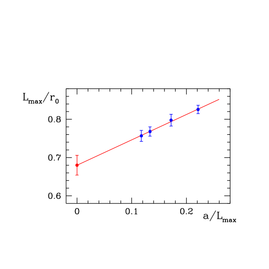
Figure 1: Extrapolation of $L_{\rm max}/r_{0}$ to the continuum limit

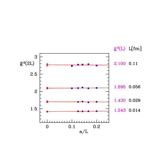
Figure 2: Extrapolation of $\Sigma$ to the continuum limit à la Symanzik

Step 2, measuring the evolution was historically done in the reverse order from the description above and the standard notation in the following is suited for this. In the continuum limit there is a well defined function $\sigma$, the step scaling function, relating the coupling at one volume to that at double the volume:

$$\bar{g}_{\mathrm{FV}}^{2}(2L)=\sigma(\bar{g}_{\mathrm{FV}}^{2}(L))\,.$$ (12)

With a lattice regularization this is modified to

$$\bar{g}_{\mathrm{FV}}^{2}(2L)=\Sigma(\bar{g}_{\mathrm{FV}}^{2}(L),a/L)\,.$$ (13)

One then starts with a convenient small lattice, say $L/a=8$, and tunes $g_{0}$ such that $\bar{g}_{\mathrm{FV}}^{2}(L)$ equals some small value $u$. At the same $g_{0}$ one computes $\bar{g}_{\mathrm{FV}}^{2}(2L)=\Sigma(u,a/L)$. One then repeats this for a manageable range of $a/L$ as illustrated in Fig. 2, and extrapolates the result to the continuum limit thus obtaining a value for $\sigma(u)=u^{\prime}$. The whole procedure is then repeated but this time starting with an initial value $\bar{g}_{\mathrm{FV}}^{2}(L)=u^{\prime}$ (or a value close to $u^{\prime}$). After this has been done many ($\mathrm{O}(10)$) times, one ends up with a sequence of points for the continuum step scaling function as illustrated in Fig. 3:

$$u_{k}=\sigma(u_{k+1})\,,\,\,\,\,u_{0}=3.48\,,$$ (14)

giving $\bar{g}_{\mathrm{FV}}^{2}(L)$ at $L=2^{-k}L_{\mathrm{max}}$. At the small values of $L$ one can check whether $\sigma(u)$ is well described by the perturbative expectation

$$\sigma(u)=u+(2\ln 2)b_{0}u^{2}+\dots$$ (15)

and if this is the case one can use the beta function with perturbative coefficients to compute $\Lambda_{\mathrm{FV}}$ in physical units. After that the steps are straightforward; a 1-loop computation relating $\alpha_{\mathrm{FV}}$ to $\alpha_{\mathrm{\overline{MS\kern-0.98pt}\kern 0.98pt}}$ yields the ratio of $\Lambda$–parameters and hence the desired value of the product $\Lambda_{\mathrm{\overline{MS\kern-0.98pt}\kern 0.98pt}}r_{0}$ relating the scales of the hadronic (LE) and perturbative (HE) renormalization schemes.

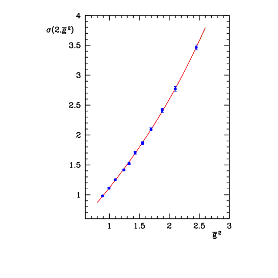
Figure 3: Results for the continuum step scaling function

It is clear that for the success of the RFS method described above, we need a definition of the coupling which satisfies the following criteria: a) it should be accurately measurable, b) it has preferably small lattice artifacts, and c) it should be relatively easily computable in PT.

3 The Schrödinger functional

After some extensive R&D members of the Alpha Collaboration found that couplings based on the Schrödinger functional (SF) satisfy the above requirements Luscher:1992an. It was further realized that the setup is also well suited for the computation of renormalization constants in general, and that it is easily extended to include fermions and to compute their running masses.

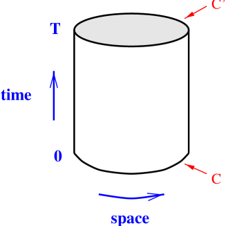
Figure 4: Geometry of the Schrödinger functional

In this framework one studies the system in a cylindrical volume $\Lambda$ with Dirichlet boundary conditions in one (the temporal) direction and periodic bc in the other (spatial) directions (illustrated in Fig. 4):

$$A_{k}({\bf x},0)=C_{k}\,,\,\,\,\,A_{k}({\bf x},T)=C^{\prime}_{k}\,,\,\,\,\,A_{k}({\bf x}+L,t)=A_{k}({\bf x},t)\,.$$ (16)

Formally in the continuum the SF is given by the functional integral

$$Z(C,C^{\prime})=\int_{SF\,\,{\rm bc}}D[A]\,\mathrm{e}^{-S}\,,$$ (17)

which is properly defined so that it is equal to the transition amplitude $\langle C^{\prime}|\mathrm{e}^{-\rm I\kern-1.39998ptHT}\rm I\kern-1.99997ptP|C\rangle$ ($\rm I\kern-1.99997ptH$ the Hamiltonian, $\rm I\kern-1.99997ptP$ the projector on gauge invariant states) in the Hamiltonian formulation.

The renormalization of the SF in scalar field theories was first studied by Symanzik Symanzik:1981wd. He found that apart from the usual renormalization of the bare parameters and fields in the bulk one just requires some extra terms on the boundaries, specifically spatial integrals over local fields of dimension $\leq 3$. Lüscher’s paper Luscher:1985iu gives a clear introduction to the subject. There are no such local gauge invariant operators in pure Yang–Mills theory and so the (bare) SF should in this case not need any renormalization besides the usual coupling constant renormalization. We remark that one of the first papers considering the related topic of the structure of Yang–Mills theories in the temporal gauge were by Rossi and Testa (Rossi:1979jf, Rossi:1980pg).

For small bare coupling $g_{0}$ the functional integral is dominated by fields around the absolute minimum of the action described by some background field $B$. The SF then has a perturbative expansion

$$-\ln Z(C,C^{\prime})\sim\Gamma(B)=g_{0}^{-2}\Gamma_{0}(B)+\Gamma_{1}(B)+\dots$$ (18)

If the boundary fields depend on a parameter $\eta$ then one can define a renormalized running coupling as

$$\bar{g}^{2}_{\rm SF}(L)=\left(\frac{\partial\Gamma_{0}(B)/\partial\eta}{\partial\Gamma(B)/\partial\eta}\right)_{\eta=0,T=L}\,.$$ (19)

Regularizing the gauge theory on the lattice the Scrödinger functional is an integral over all configurations of link matrices in ${\rm SU}(N)$:

$$Z(C,C^{\prime})=\int D[U]\mathrm{e}^{-S[U]}\,,$$ (20)

with the Haar measure and the $U$ satisfying periodic boundary conditions in the spatial directions and Dirichlet bc in the time direction:

$$U(x,k)|_{x_{0}=0}=W(x,k)\,,\,\,\,\,U(x,k)|_{x_{0}=T}=W^{\prime}(x,k)\,,\,\,\,\,k=1,2,3\,,$$ (21)

where

$$W(x,k)={\mathcal{P}}\exp\left\{a\int_{0}^{1}\mathrm{d}t\,C_{k}\left(x+(1-t)a\hat{k}\right)\right\}\,,$$ (22)

i.e. the SF is considered as a functional of the continuum fields $C,C^{\prime}$ and the continuum limit $a\to 0$ is taken with $C,C^{\prime}$ fixed.

One can work in principle with any acceptable lattice action, the simplest being Wilson’s plaquette action

$$S=\frac{1}{g_{0}^{2}}\sum_{p}w(p)\Re\,\mathrm{tr}\,(1-U(p))\,,$$ (23)

where the sum is over all plaquettes $p$ and the weight $w(p)=1$ except for those lying on the boundary which is chosen $w(p)=1/2$ to avoid a classical $\mathrm{O}(a)$ effect.

Note that the derivative entering the definition of the coupling is

$$\frac{\partial\Gamma}{\partial\eta}=\left\langle\frac{\partial S}{\partial\eta}\right\rangle\,.$$ (24)

The expectation value appearing on the rhs involves only “plaquettes” localized on the boundary. These are accurately measurable hence satisfying criteria (a) above.

As for the particular choice of the boundary fields $C,C^{\prime}$ to make the perturbation expansion well defined we need the following stability condition: if $V(x,\mu)=\exp\left[aB_{\mu}(x)\right]$ is a configuration of least action (with bc $C,C^{\prime}$) then any other gauge field with the same action is gauge equivalent to $V$. Secondly we would like to have criterion (b). How to make optimal choices satisfying these demands is not at all obvious. Again after some experimentation the Alpha Collaboration made the choice of abelian bc e.g. for SU(3):

$$C_{k}(x)=\frac{i}{L}\left(\begin{array}[]{ccc}\phi_{1}&0&0\\ 0&\phi_{2}&0\\ 0&0&\phi_{3}\\ \end{array}\right)\,,\,\,\,\,\sum_{\alpha=1}^{3}\phi_{\alpha}=0\,,\,\,\,\phi_{\alpha}\,\,{\rm indep.\,\,of}\,\,x,k\,,$$ (25)

and similarly for $C^{\prime}$ involving elements $\phi^{\prime}_{i}$. The induced background field is abelian and given by ($T=L$)

$$B_{0}=0\,,\,\,\,B_{k}(x)=C+(C^{\prime}-C)x_{0}/L\,,\,\,\,\,C=C(\eta)\,.$$ (26)

Stability has been proven Luscher:1992an provided the $\phi$’s satisfy

$$\phi_{1}<\phi_{2}<\phi_{3}\,,\,\,\,\,|\phi_{\alpha}-\phi_{\beta}|<2\pi\,,$$

(and similarly for $\phi^{\prime}_{\alpha}$), and provided $TL/a^{2}$ is large enough, albeit the bound not being very restrictive e.g. $TL/a^{2}>2\pi^{2}$ for $N=3$.

With this setup the Alpha Collaboration produced measurements of a running coupling (in the continuum limit as far as it could be controlled) over a large range of energies , as depicted in Fig. 5. At high energies the running is consistent with perturbative expectations, giving convincing numerical support to the (yet unproven) conventional wisdom that the critical coupling is $g_{c}=0$ and that the continuum limit of the lattice theory is asymptotically free . Contrary to widespread opinion the latter property is non-trivial (so far lacking rigorous proof) and some authors have questioned its validity Patrascioiu:2000mw.

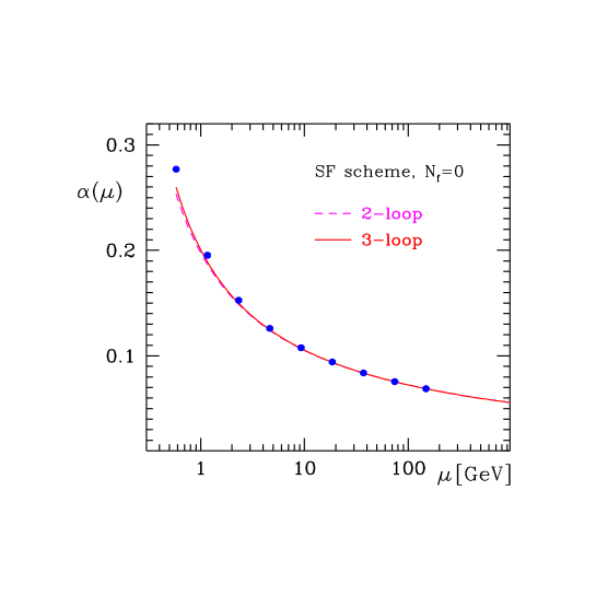
Figure 5: SF running coupling $\alpha(\mu)=\bar{g}^{2}_{\rm SF}(L)/4\pi\,,\,\,\mu=1/L$ ($N_{\mathrm{f}}=0$)

4 Inclusion of fermions

The inclusion of fermions in the SF framework was first considered by Sint (Sint:1993un, Sint:1995rb). In the continuum it has been argued by Lüscher Luscher:2006df that “natural boundary conditions” involve linear conditions for the fields of lowest dimension. For Dirac fermions these take the form

$$\mathcal{B}\psi|_{\rm bdy}=0$$ (27)

where, in order to obtain a non-trivial propagator, the matrix $\mathcal{B}$ must not have maximal rank. If one demands invariance under space, parity, time reflections ($x_{0}\to T-x_{0}$) and charge conjugation, one is left with the possibility

$$P_{+}\psi(x)=\overline{\psi}(x)P_{-}=0\,,\,\,\,x_{0}=0\,;\,\,\,P_{-}\psi(x)=\overline{\psi}(x)P_{+}=0\,,\,\,\,x_{0}=T\,,$$ (28)

(or $P_{+}\leftrightarrow P_{-}$) where $P_{\pm}=\frac{1}{2}(1\pm\gamma_{0})$. Sint showed that with these homogeneous boundary conditions the SF is renormalizable without the necessity of including any extra boundary terms.

With the lattice regularization where continuity considerations are a priori missing, boundary conditions are implicit in the specification of the dynamical fields (those to be integrated in the functional integral) and the precise form of the action close to the boundary. For Wilson fermions the terms in the action coupling close to the boundary e.g. near $x_{0}=0$ have the form $\propto\overline{\psi}(a)P_{+}\psi(0)+\overline{\psi}(0)P_{-}\psi(a)$. It is thus natural in the corresponding lattice SF to declare fields $\psi(x),\overline{\psi}(x)$ away from the boundary i.e. $0<x_{0}<T$ as the dynamical variables and expect that the bc’s (28) are recovered dynamically in the continuum limit. Often in the SF literature one sees the equations

$$P_{+}\psi(0,{\bf x}) = \rho({\bf x})\,,\,\,\,\,\overline{\psi}(0,{\bf x})P_{-}=\bar{\rho}({\bf x})\,,\,\,\,\,$$

$$P_{-}\psi(T,{\bf x}) = \rho^{\prime}({\bf x})\,,\,\,\,\,\overline{\psi}(T,{\bf x})P_{+}=\bar{\rho}^{\prime}({\bf x})\,.$$

These are however not to be considered as specifying boundary conditions, but describe couplings of sources for the undefined field components near the boundary. For example, defining

$$\xi({\bf x})=P_{-}\frac{\delta}{\delta\bar{\rho}({\bf x})}\,,\,\,\,\bar{\xi}({\bf x})=-\frac{\delta}{\delta\rho({\bf x})}P_{+}\,,$$ (29)

we can consider correlation functions of the form

$$\langle\mathcal{O}^{a}A^{a}(x)\rangle\sim\int[\mathrm{d}U\,\mathrm{d}\psi\,\mathrm{d}\overline{\psi}]\,\mathcal{O}^{a}A^{a}(x)\mathrm{e}^{-S}|_{\rho=\bar{\rho}=\rho^{\prime}=\bar{\rho}^{\prime}=0}\,,$$ (30)

where all sources are set to zero after differentiating and

$$\mathcal{O}^{a}\equiv-\sum_{{\bf y},{\bf z}}\bar{\xi}({\bf y})\frac{1}{2}\tau^{a}\gamma_{5}\xi({\bf z})\,.$$ (31)

In this setting the extra boundary counter-terms appearing in Sint’s original paper amount to a renormalization of the sources $\xi({\bf x})\to Z^{1/2}_{\xi}\xi({\bf x})$.

An important point is that the SF fermion boundary conditions imply a gap in the spectrum of the Dirac operator at least for $g_{0}$ small enough. This has the consequence that simulations at zero quark mass $m_{\mathrm{q}}=0$ with the Schrödinger functional are not problematic.

Also an extra option is to impose quasi-periodic boundary conditions in the spatial direction of the form

$$\psi(x+L\hat{k})=\mathrm{e}^{i\theta_{k}}\psi(x)\,,\,\,\,\,\overline{\psi}(x+L\hat{k})=\mathrm{e}^{-i\theta_{k}}\overline{\psi}(x)\,,$$ (32)

which are equivalent to modifying the covariant derivative to

$$(\nabla_{k}\psi)(x)=\frac{1}{a}\left[\mathrm{e}^{ia\theta_{k}/L}U(x,k)\psi(x+a\hat{k})-\psi(x)\right]\,,$$ (33)

and similarly for $\nabla_{k}^{*}$. Such boundary conditions with various choices of the $\theta_{k}$ serve as extra probes of the system.

Chapter 3 Lattice artifacts

Probably in the future, computers will be so powerful that physically large enough lattices will be measurable with very small lattice spacing $a$, such that lattice artifacts become numerically irrelevant. Even so the question of the nature of lattice artifacts is of theoretical interest. However, at present it is important in practice to gain insight in the form of the artifacts in order to make reliable extrapolations of numerical data to the continuum limit.

Usually we make extrapolations of e.g. ratios of masses of the form (2) assuming leading artifacts are predominantly polynomial in the lattice spacing. Lattice artifacts are non-universal e.g. the exponent $p$ and the coefficient $C_{12}$ in (2) depend on the lattice action. This can be used in various ways e.g. if we simulate different actions and the data for glueball masses looks as in Fig. 1, this would be a support of the (expected) universality of the continuum limit and one could make a constrained joint fit.

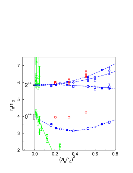
Figure 1: An old plot of glueball masses in pure YM measured with different actions Morningstar:1996dn; the results indicate universality. Green points (plaquette action) and the others from improved actions.

More ambitious ways of using the non-universality involve designing actions with larger values of the exponent $p$, which are called Symanzik improved actions (Symanzik:1979ph, Symanzik:1981hc) or even constructing perfect actions having in principle $p=\infty$ (see sect. 6).

Again most of our knowledge concerning lattice artifacts comes from studies of perturbation theory. Some non-perturbative support for the validity of the structure found there comes from investigations in the $1/n$-expansion of QFT in 2 dimensions (see Knechtli:2005jh, Wolff:2005nf and references therein), and also from many numerical simulations.

1 Free fields

Let us first consider a free scalar field theory on an infinite 4–dimensional hyper-cubic lattice with standard action:

$$S_{0}=a^{4}\sum_{x,\mu}\frac{1}{2}\left[\partial_{\mu}\phi(x)\partial_{\mu}\phi(x)+m^{2}\phi(x)^{2}\right]\,,$$ (1)

where $\partial_{\mu}f(x)=\left[f(x+a\hat{\mu})-f(x)\right]/a$. The 2–point function is

$$\widetilde{G}(k)=\frac{1}{\hat{k}^{2}+m^{2}}\,,$$ (2)

where $\hat{k}_{\mu}=\frac{2}{a}\sin\frac{ak_{\mu}}{2}$. Noting that for small $a$,

$$\hat{k}^{2}=k^{2}-\frac{1}{12}a^{2}\sum_{\mu}k_{\mu}^{4}+\mathrm{O}(a^{4})\,,$$ (3)

we can write ($\phi_{0}$ the corresponding field in the continuum theory)

$$\widetilde{G}(k)=\widetilde{G}_{\mathrm{cont}}(k)-a^{2}\langle S_{1}^{\mathrm{eff}}\widetilde{\phi}_{0}(k)\phi_{0}(0)\rangle+\dots$$ (4)

with

$$S_{1}^{\mathrm{eff}}=-\int\mathrm{d}^{4}x\,\sum_{\mu}\frac{1}{24}\partial_{\mu}^{2}\phi_{0}(x)\partial_{\mu}^{2}\phi_{0}(x)\,.$$ (5)

On–shell information is obtained from the (lattice) two point function $G(x)$ when $x$ is separated from 0 by a physical distance. Performing the integral over $k_{0}$ we obtain the representation

$$G(x)=\int^{\pi/a}_{-\pi/a}\frac{\mathrm{d}^{3}k}{(2\pi)^{3}}\,\mathrm{e}^{i{\bf k}{\bf x}}\,\frac{\mathrm{e}^{-\epsilon({\bf k},a,m)x_{0}}}{R({\bf k},m)}\,,$$ (6)

where the energy spectrum $\epsilon({\bf k},a,m)$ is given by

$$\cosh(a\epsilon({\bf k},a,m))-1=\frac{1}{2}a^{2}\left(\hat{{\bf k}}^{2}+m^{2}\right)\,.$$ (7)

Defining the pole mass by $m_{\mathrm{p}}=\epsilon(0,a,m)$ we obtain in the continuum limit $a\to 0$, $m_{\mathrm{p}}$ fixed:

$$\epsilon({\bf k},a,m)^{2}=m_{\mathrm{p}}^{2}+{\bf k}^{2}-\frac{a^{2}}{12}T({\bf k},m_{\mathrm{p}})+\mathrm{O}(a^{4})\,;\,\,T({\bf k},m_{\mathrm{p}})=\sum_{j}k_{j}^{4}+{\bf k}^{2}\left({\bf k}^{2}+2m_{\mathrm{p}}^{2}\right)\,.$$ (8)

The cutoff effects are (for $m_{\mathrm{p}}=0$) of order $>10\%$ for $k>2\pi/(5a)$. One can improve this situation by adding $\mathrm{O}(a^{2})$ terms to the action. This can be done in many ways, the simplest possibility being

$$S = S_{0}+cS_{1}\,,$$ (9)

$$S_{1} = a^{4}\sum_{x,\mu}\frac{a^{2}}{2}\partial_{\mu}^{2}\phi(x)\partial_{\mu}^{2}\phi(x)\,,$$ (10)

the latter involving interaction of next-to-nearest neighbors. The energy spectrum is now given by the solution to

$$\cosh(a\epsilon({\bf k},a,m))-1-2c\left[\cosh(a\epsilon({\bf k},a,m))-1\right]^{2}=\frac{1}{2}a^{2}\left(\hat{{\bf k}}^{2}+m^{2}+ca^{4}\sum_{j}\hat{k}_{j}^{4}\right)\,.$$ (11)

Now for small lattice spacing $a$ the energy spectrum has the form

$$\epsilon({\bf k},a,m)^{2}=m_{\mathrm{p}}^{2}+{\bf k}^{2}+\left(c-\frac{1}{12}\right)a^{2}T({\bf k},m_{\mathrm{p}})+\mathrm{O}(a^{4})\,,$$ (12)

from which we see that the energy is $\mathrm{O}(a^{2})$ improved if we chose $c=\frac{1}{12}$.

Note that for the improved action another energy level is present but its real part always remains close to the cutoff, and hence it is irrelevant for the continuum limit

Exercise 1.1.

What is $S_{1}^{\mathrm{eff}}$ for the action

$$S_{0}+cS_{1}+d\sum_{x,\mu,\nu}\frac{a^{2}}{2}\partial_{\mu}^{*}\partial_{\mu}\phi(x)\partial_{\nu}^{*}\partial_{\nu}\phi(x)\,.$$

Show that the energy is improved for $c=\frac{1}{12}$ for arbitrary $d$.

2 Symanzik’s effective action

Based on low order perturbative computations in various field theories one arrives at the following conjecture: In a large class of interacting lattice theories (in particular asymptotically free theories) there exists an (Symanzik’s) effective continuum action

$$S_{1}^{\mathrm{eff}}=\int\mathrm{d}^{d}y\,\mathcal{L}_{1}(y)\,,$$ (13)

such that a Green function of products of a multiplicatively renormalizable lattice field $\varphi$ at widely separated points $x_{i}$ takes the form

$$Z_{\varphi}^{r/2}\langle\varphi(x_{1})\dots\varphi(x_{r})\rangle_{\rm latt}=\langle\varphi_{0}(x_{1})\dots\varphi_{0}(x_{r})\rangle_{\rm cont}$$

$$-a^{p}\int\mathrm{d}^{d}y\,\langle\mathcal{L}_{1}\varphi_{0}(x_{1})\dots\varphi_{0}(x_{r})\rangle_{\rm cont}$$

$$+a^{p}\sum_{k=1}^{r}\langle\varphi_{0}(x_{1})\dots\varphi_{1}(x_{k}))\dots\varphi_{0}(x_{r})\rangle_{\rm cont}+\dots$$ (14)

where $\varphi_{0},\varphi_{1}$ are renormalized continuum fields, in particular $\varphi_{1}$ is a sum of local operators of dimension $d_{\varphi}+p$ depending on the specific operator $\varphi$ and having the same lattice quantum numbers as $\varphi$. The effective Lagrangian is a sum

$$\mathcal{L}_{1}=\sum_{i}c_{i}(g(\mu),a\mu)\mathcal{O}_{\mathrm{R}i}(\mu)\,,$$ (15)

of local operators $\mathcal{O}_{\mathrm{R}i}$ of dimension $d+p$ having the symmetries of the lattice action. $\mu$ is the renormalization scale e.g. of the dimensional regularization used in the continuum.

Note a) in the integral over $y$ one in general encounters singularities at points $y=x_{k}$. A subtraction prescription must thus be applied, but the arbitrariness in this procedure amounts to a redefinition of $\varphi_{1}$. b) The coefficients $c_{i}$ are, as indicated, functions of the lattice spacing $a$, but the dependence is thought to be weak (logarithmic).

If the conjecture is true then one generically expects $\mathrm{O}(a^{2})$ artifacts in pure Yang–Mills theory and $\mathrm{O}(a)$ effects with Wilson fermions. All present numerical data seems consistent with these expectations but until now only a small range of $a$ is available.

3 Logarithmic corrections to $\mathrm{O}(a^{2})$ lattice artifacts

In 2d lattice models e.g. the non-linear O($n$) sigma model, which is perturbatively asymptotically free, one can simulate lattices with very large correlation lengths ($>200a$). In these theories the expectation is also $\mathrm{O}(a^{2})$ artifacts. Hence it came as a surprise, as mentioned by Hasenfratz in his LATT2001 plenary talk Hasenfratz:2001bz, that data on a step scaling function in this model seemed to show $\mathrm{O}(a)$ effects as illustrated in Fig. 2! This was rather unsettling and motivated Balog, Niedermayer and myself (Balog:2009np, Balog:2009yj) to investigate the logarithmic corrections to the $\mathrm{O}(a^{2})$ in the framework of renormalized perturbation theory. We found that generic artifacts in the $\mathrm{O}(n)$ sigma model are of the form $a^{2}\ln^{s}(a^{2})$ with $s=n/(n-2)$. For $n=1$ the exponent is $s=3$, and such strong logarithmic corrections to the $\mathrm{O}(a^{2})$ effects can explain the peculiar behavior, and yield good fits of the data for various actions Balog:2009np. For $n=\infty$ the exponent is $s=1$ which is consistent with what is found in leading orders of the $1/n$ expansion Wolff:2005nf.

Figure 2: Monte Carlo measurements of the O(3) $\sigma$–model step scaling function at $u_{0}=1.0595$ for two lattice actions. The fits shown contain $a$ and $a\ln a$ terms. Fits of the form $k_{1}a^{2}+k_{2}a^{2}\ln a+k_{3}a^{4}$ have unacceptably high $\chi^{2}/{\rm dof}$.

The steps involved in obtaining the result above are as follows.

1) Classify operators of dimension 4 (recall for this case $d=2$ and $p=2$) which appear in the Symanzik effective Lagrangian (15).

2) Compute the $c_{i}$ at tree level (the coefficients normalized such that $c_{i}=c_{i}^{(0)}+\mathrm{O}(g^{2})$). Although finally interested only in on–shell observables, it is sometimes convenient to work off shell and compute a sufficient number of correlation functions $G^{(r)}$ with a product of $r$ basic fields, in the continuum and on the lattice. For the lattice Green function,

$$G^{(r)}_{\rm latt}=G^{(r)}_{\rm cont}+a^{2}\sum_{i}c_{i}(g)G^{(r)}_{i}+\dots$$ (16)

where $G_{i}^{(r)}$ are continuum correlation functions involving additional insertion of a composite field $\mathrm{O}_{\mathrm{R}i}$.

3) The ratios $\delta^{(r)}_{i}=G^{(r)}_{i}/G^{(r)}$ which characterize the lattice artifacts (but are themselves independent of the lattice regularization) obey an RG equation of the form

$$\left\{\left(-a\frac{\partial}{\partial a}+\beta\frac{\partial}{\partial g}\right)\delta_{ij}+\nu_{ij}\right\}\delta^{(r)}_{j}=0\,,$$ (17)

where $\nu_{ij}$ is obtained from the mixing of the $\mathrm{O}_{\mathrm{R}i}$ to 1-loop (see sect. 2.3). If we have a basis where the renormalization is diagonal to one loop $\nu_{ij}=-2b_{0}\triangle_{i}\delta_{ij}g^{2}+\dots$ then the operator associated to the largest value of $\triangle_{i}$ generically dominates the artifacts if the corresponding tree level coefficient $c_{i}(0)\neq 0$.

The program should be carried out for lattice actions used for large scale simulations of QCD, when technically possible, in order to check if potentially large logarithmic corrections to lattice artifacts predicted by perturbative analysis appear.

4 Symanzik improved lattice actions

If Symanzik’s conjecture is true it practically follows that it is possible to find a Symanzik improved lattice action such that $S_{1}^{\rm eff}=0$, i.e. for this action there are no lattice artifacts $\mathrm{O}(a^{p})$. The conjecture is generally accepted for AF theories, but I should mention that a rigorous proof of the existence of a Symanzik improved lattice action for any theory (including $\phi^{4}$) to all orders PT is, to my knowledge, not complete. But there is an all order proof by Keller Keller:1992xm for the existence of Symanzik improved actions for $\phi^{4}_{4}$ and QED in the framework of a continuum regularization (using flow equations) . A subtle point is that the continuum limit of lattice $\phi^{4}_{4}$ theory is probably trivial i.e. a free theory. The renormalized coupling goes to zero as $c/\ln(a\mu)$ and hence the continuum limit is actually reached only logarithmically! Treating the renormalized coupling $g$ effectively as a constant for a range of cutoffs one has for small $g$ a perturbative Lagrangian description of the low energy physics, and in this case the Symanzik effective Lagrangian describes the leading cutoff corrections to this.

An important ingredient of a lattice proof (to all orders PT) would presumably need a proof of the small $a$ expansion of an arbitrary $\ell$–loop Feynman diagram of the form

$$F(p,a)\sim a^{-\omega}\sum_{n=0}^{\infty}a^{n}\sum_{r=0}^{\ell}(\ln am)^{r}F_{nr}(p)\,,$$ (18)

which we are quite confident holds and hence often stated in the literature, but which again has not, to my knowledge, been proven for $\ell\geq 2$.

Exercise 4.1.

As an example of an expansion of the form (18), consider a lattice $\phi^{4}_{4}$ theory with free propagator $1/[R(k,a)+m^{2}]$ with

$$R(q/a,a)=a^{-2}r(q)\,,\,\,\,\,r(q)\sim_{q=0}q^{2}+c(q^{2})^{2}+d\sum_{\mu}q_{\mu}^{4}+\dots$$

Show that the tadpole integral $J_{1}=\int_{-\pi/a}^{\pi/a}\mathrm{d}^{4}k\,[R(k,a)+m^{2}]^{-1}$ has an expansion of the form

$$J_{1}\sim a^{-2}\left\{r_{0}+a^{2}m^{2}[r_{1}+s_{1}\ln(am)]+a^{4}m^{4}[r_{2}+s_{2}\ln(am)]+\mathrm{O}(a^{6})\right\}$$

with $s_{2}=0$ if $c=d=0$.

5 On–shell improved action for pure Yang–Mills theory

Figure 3: 4 and 6-link closed curves on the lattice

With the insight gained from our previous discussion we are now prepared to consider improved actions for Yang–Mills theory in 4 dimensions Luscher:1984zf. As by now familiar, the first step is to classify the independent (up to total derivatives) gauge invariant operators of dimension 6, which are scalars under lattice rotations; there are three such operators Weisz:1982zw:

$$O_{1}=\sum_{\mu,\nu}\mathrm{tr}D_{\mu}F_{\mu\nu}D_{\mu}F_{\mu\nu}\,,\,\,O_{2}=\sum_{\mu,\nu,\rho}\mathrm{tr}D_{\mu}F_{\nu\rho}D_{\mu}F_{\nu\rho}\,,\,\,O_{3}=\sum_{\mu,\nu,\rho}\mathrm{tr}D_{\mu}F_{\mu\rho}D_{\nu}F_{\nu\rho}\,,$$ (19)

where $D_{\mu}F_{\nu\rho}=\partial_{\mu}F_{\nu\rho}+g_{0}\left[A_{\mu},F_{\nu\rho}\right]$. Candidates for Symanzik improved actions have the form

$$S_{\rm imp} = \frac{2}{g_{0}^{2}}\sum_{i}c_{i}(g_{0})\sum_{\mathcal{C}_{i}\in\mathcal{S}_{i}}\mathcal{L}(\mathcal{C}_{i})\,,$$ (20)

$$\mathcal{L}(\mathcal{C}) = \Re\,\mathrm{tr}\,[1-U(\mathcal{C})]\,,$$ (21)

where $U(\mathcal{C})$ is the ordered product of link variables around the closed curves $\mathcal{C}$, and $\mathcal{S}_{i}$ are sets with a given topology e.g. $\mathcal{S}_{0}=$ the set of plaquettes,
$\mathcal{S}_{1}=$ the set of $2\times 1$ rectangles, $\mathcal{S}_{2}=$ the set of “twisted chairs”,
$\mathcal{S}_{3}=$ the set of “chairs”, as depicted in Fig. 3.
Identifying the $U(x,\mu)$ with phase factors in the continuum associated with the links as in (22) (with $C_{k}$ replaced by $g_{0}A_{\mu}$), the classical small $a$ expansion of the local lattice operators is given by

$$\mathcal{O}_{i}(x) \equiv \frac{1}{4}\sum_{\mathcal{C}\in\mathcal{S}_{i},x\in\mathcal{C}}\mathcal{L}(\mathcal{C})$$ (22)

$$= a^{4}z_{i}\mathrm{tr}F_{\mu\nu}F_{\mu\nu}+a^{6}\sum_{j=1}^{3}p_{ij}O_{j}(x)\,.$$ (23)

We need only 4 lattice operators to represent the 4 continuum operators of dimension 4,6 appearing in the effective action. We chose the sets of curves with smallest perimeter $\leq 6$ mentioned above, but many other choices are admissible (and have appeared in the literature). In order that the coefficient of $F^{2}$ in the classical expansion has the usual normalization the coefficients must satisfy

$$c_{0}(g_{0})+8c_{1}(g_{0})+8c_{2}(g_{0})+16c_{3}(g_{0})=1\,.$$ (24)

Further one finds that improvement of the classical action requires

$$c_{1}(0)=-\frac{1}{12}\,,\,\,\,\,\,c_{2}(0)=c_{3}(0)=0\,.$$ (25)

On the other hand improvement of on-shell quantities only requires two conditions among the coefficients. e.g. for the static 2-quark potential at tree level one finds

$$V(R)=-C\frac{g_{0}^{2}}{4\pi R}\left[1+3\left(c_{1}(0)-c_{2}(0)-c_{3}(0)-\frac{1}{12}\right)\frac{a^{2}}{R^{2}}+\dots\right]\,.$$ (26)

Spectral quantities in finite volumes, e.g. with twisted boundary conditions, can also be computed, and reproduces the improvement condition above and in addition the condition $c_{2}(0)=0$ (Luscher:1984xn, Luscher:1984xo). There are no other independent relations. This is as expected because on-shell the operator $O_{3}$ can be dropped from the effective action since it vanishes when using the equations of motion. For on-shell improvement we conclude that we can choose

$$c_{3}(g_{0})=0\,\,\,\,\,{\rm for\,\,all\,\,}g_{0}\,.$$ (27)

The coefficients $c_{i}$ can be computed to higher orders in PT. To 1-loop they have been computed from the same observables as mentioned above Luscher:1985zq.

In principle the $c_{i}(g_{0})$ could be computed non-perturbatively by demanding cutoff effects to vanish from some spectral levels e.g. requiring the $J^{\rm PC}=2^{++}$ states to be degenerate. This has not been done yet, the reason being that the physical goal is QCD and to achieve full $\mathrm{O}(a^{2})$ improvement in that theory is much more difficult because there are more dimension $6$ operators to be taken into account, in particular those involving products of 4 quark fields. Never the less improved gauge actions, based on various considerations, are used in practical large scale numerical simulations.

Chapter 4 $\mathrm{O}(a)$ improved Wilson fermions

As discussed in Hernandez’ lectures, there are many ways of putting fermions on the lattice, each having their own particular advantages and disadvantages. In this section I will only discuss lattice artifacts with Wilson fermions. From the tree level coupling of quarks to one gluon

$$\sim g_{0}T^{a}\left\{\gamma_{\mu}-\frac{1}{2}a(p+p^{\prime})_{\mu}+\mathrm{O}(a^{2})\right\}\,,$$ (1)

we immediately see that there are $\mathrm{O}(a)$ off–shell effects, and some persist on–shell. The on-shell $\mathrm{O}(a)$ improvement program Luscher:1996ug proceeds on the same lines as for the pure gauge fields in the last section. The first step is thus to classify the independent local gauge invariant operators of dimension 5 that can occur in the effective Lagrangian $\mathcal{L}_{1}$:

$$O_{1} = g_{0}\overline{\psi}i\sigma_{\mu\nu}F_{\mu\nu}\psi\,,\,\,\,\,\sigma_{\mu\nu}=\frac{i}{2}\left[\gamma_{\mu},\gamma_{\nu}\right]\,,\,\,\,$$ (2)

$$O_{2} = \overline{\psi}D_{\mu}D_{\mu}\psi+\overline{\psi}\overleftarrow{D}_{\mu}\overleftarrow{D}_{\mu}\psi\,,\,\,\,\,\,\,\overline{\psi}\overleftarrow{D}_{\mu}=\overline{\psi}\left(\overleftarrow{\partial}_{\mu}-g_{0}A_{\mu}\right)\,,$$ (3)

$$O_{3} = mg_{0}^{2}\mathrm{tr}F_{\mu\nu}F_{\mu\nu}\,,\,\,\,\,O_{4}=m\overline{\psi}\left(D_{\mu}-\overleftarrow{D}_{\mu}\right)\gamma_{\mu}\psi\,,\,\,\,O_{5}=m^{2}\overline{\psi}\psi\,.$$ (4)

On-shell we can use the equations of motion $(\gamma D+m)\psi=0$ to derive relations

$$O_{1}-O_{2}+2O_{5}\simeq 0\,,\,\,\,\,O_{4}+2O_{5}\simeq 0\,,\,\,\,\,$$ (5)

which can be used to eliminate $O_{2},O_{4}$. A Symanzik–improved action should then be constructible by adding a linear combination of lattice representations of $O_{1},O_{3},O_{5}$

$$\delta S=a^{5}\sum_{x}\left\{c_{1}(g_{0})\widehat{O}_{1}(x)+c_{3}(g_{0})\widehat{O}_{3}(x)+c_{5}(g_{0})\widehat{O}_{5}(x)\right\}\,,$$ (6)

to the Wilson fermion action. Now $\widehat{O}_{3},\widehat{O}_{5}$ are already present in the original lattice action, so adding these terms merely corresponds to a rescaling of the bare coupling and masses by terms $\sim 1+\mathrm{O}(am)$. i.e. they can be dropped until we discuss renormalization. We conclude that the on-shell improved Wilson action has only one extra term

$$S_{\rm imp}=S_{W}+a^{5}\sum_{x}c_{\rm SW}(g_{0})\overline{\psi}(x)\frac{i}{4}\sigma_{\mu\nu}\widehat{F}_{\mu\nu}(x)\psi(x)\,,$$ (7)

where the lattice representative $\widehat{F}_{\mu\nu}(x)$ of $g_{0}F_{\mu\nu}(x)$ depicted in Fig. 1 has a “clover-leaf form” . This action was first written down by Sheikholeslami and Wohlert Sheikholeslami:1985ij. The coefficient $c_{\rm SW}(g_{0})$ is known to 1-,2-loop order of PT for various gauge actions.

$\widehat{F}_{\mu\nu}(x)\,\,\,\,\propto\,\,\,$

Figure 1: Lattice representative of $g_{0}F_{\mu\nu}$

Two comments are in order here. Firstly as for any improvement, $\mathrm{O}(a)$ improvement is only an asymptotic concept; it could happen that at some $g_{0}$ we have bad luck and $\mathrm{O}(a^{2})$ effects are bigger than $\mathrm{O}(a)$ effects for some quantities. Secondly, a rather nice feature is that the extra overhead CPU cost in simulations of adding a SW term is not very substantial.

1 $\mathrm{O}(a)$ improvement of operators

In order to eliminate lattice artifacts in correlation functions involving composite operators, we must also improve the operators themselves, by adding local terms of higher dimension having the same quantum numbers. For example for the axial iso-vector current $A_{\mu}^{a}$ the dimension 4 operator $(A_{\mu}^{a})_{1}$ in the effective Lagrangian description could involve terms

$$O^{a}_{1\mu} = \overline{\psi}\left(D_{\nu}-\overleftarrow{D}_{\nu}\right)\sigma_{\mu\nu}\gamma_{5}\frac{1}{2}\tau^{a}\psi\,,$$ (8)

$$O^{a}_{2\mu} = \partial_{\mu}\overline{\psi}\gamma_{5}\frac{1}{2}\tau^{a}\psi=\partial_{\mu}P^{a}\,,\,\,\,\,\,\,\,O^{a}_{3\mu}=mA_{\mu}^{a}\,.$$ (9)

On-shell one can eliminate $O^{a}_{1\mu}$ in favor of $O^{a}_{2\mu},O^{a}_{3\mu}$; moreover $O^{a}_{3\mu}$ is just a renormalization of the original operator. An ansatz for an improved lattice bare operator is then

$$\left(A_{I}^{a}\right)_{\mu}=A^{a}_{\mu}+ac_{\mathrm{A}}\frac{1}{2}\left(\partial_{\mu}+\partial_{\mu}^{*}\right)P^{a}\,,$$ (10)

and similarly for other operators e.g.

$$P_{I}^{a}=P^{a}\,,\,\,\,\,\left(V_{I}^{a}\right)_{\mu}=V^{a}_{\mu}+ac_{\mathrm{V}}\frac{1}{2}\left(\partial_{\nu}+\partial_{\nu}^{*}\right)i\overline{\psi}\sigma_{\mu\nu}\frac{1}{2}\tau^{a}\psi\,.$$ (11)

The improvement coefficients $c_{\mathrm{V}},c_{\mathrm{A}}$ appearing above are $\mathrm{O}(g_{0}^{2})$.

2 Mass independent renormalization scheme

In lattice QCD it is often advantageous to use a mass independent renormalization scheme as discussed in sect. 2. Without $\mathrm{O}(a)$ improvement this would involve renormalization constants independent of the quark masses and take the form

$$g_{\mathrm{R}}^{2} = g_{0}^{2}Z_{g}(g_{0}^{2},a\mu)\,,$$ (12)

$$m_{\mathrm{R}} = m_{\mathrm{q}}Z_{m}(g_{0}^{2},a\mu)\,,\,\,\,\,m_{\mathrm{q}}=m_{0}-m_{\mathrm{c}}\,.$$ (13)

To obtain correlation functions at physical distances to approach their continuum limit at a rate $\mathrm{O}(a^{2})$ with improved Wilson fermions, we must modify the form of the renormalized parameters (and thereby account for the terms $\widehat{O}_{3},\widehat{O}_{5}$ we dropped previously) in order to avoid uncanceled $\mathrm{O}(am_{\mathrm{q}})$ effects Luscher:1996ug. We do this by introducing modified bare parameters

$$\widetilde{g}_{0}^{2} = g_{0}^{2}\left(1+b_{\mathrm{g}}am_{\mathrm{q}}\right)\,,$$ (14)

$$\widetilde{m}_{\rm q}^{2} = m_{\mathrm{q}}\left(1+b_{\mathrm{m}}am_{\mathrm{q}}\right)\,,$$ (15)

and define renormalized parameters through

$$g_{\mathrm{R}}^{2} = \widetilde{g}_{0}^{2}Z_{g}(\widetilde{g}_{0}^{2},a\mu)\,,$$ (16)

$$m_{\mathrm{R}} = \widetilde{m}_{\rm q}Z_{m}(\widetilde{g}_{0}^{2},a\mu)\,.$$ (17)

We can compute the new improvement coefficients in perturbation theory. e.g. from the “pole mass” at tree level

$$m_{\rm P}=\frac{1}{a}\ln(1+am_{0})=m_{\mathrm{q}}-\frac{1}{2}am_{\mathrm{q}}+\dots\,,$$ (18)

we deduce

$$b_{\mathrm{m}}=-\frac{1}{2}+\mathrm{O}(g_{0}^{2})\,.$$ (19)

The lowest contribution to the coefficient $b_{\mathrm{g}}$ is $\mathrm{O}(g_{0}^{2})$ and first obtained by Sint and Sommer Sint:1995ch from the 1-loop computation of the SF coupling with fermions at fixed $z=m_{\mathrm{q}}L$:

$$\bar{g}_{\rm SF}^{2}(L)=g_{0}^{2}+g_{0}^{4}\left[2b_{0}\ln(L/a)+C(z)+N_{\mathrm{f}}kam_{\mathrm{q}}+\dots\right]\,,$$ (20)

from which one deduces $b_{\mathrm{g}}=N_{\mathrm{f}}kg_{0}^{2}+\dots$.

Similar factors are required for renormalized composite operators

$$A_{{\rm R}\mu}^{a} = Z_{\mathrm{A}}\left(1+b_{\mathrm{A}}am_{\mathrm{q}}\right)(A_{I}^{a})_{\mu}\,,$$ (21)

$$P_{\rm R}^{a} = Z_{\mathrm{P}}\left(1+b_{\mathrm{P}}am_{\mathrm{q}}\right)P^{a}\,.$$ (22)

The coefficients $b_{\mathrm{A}},b_{\mathrm{P}}=1+\mathrm{O}(g_{0}^{2})$, which were first computed to 1-loop order by Gabrielli:1990us, don’t depend on renormalization conditions - the latter are applied at $m_{\mathrm{q}}=0$.

3 Determination of RGI masses and running masses

We recall from sect. 2 that renormalization group invariant masses are scheme independent. Running quark masses can be defined non-perturbatively in various ways; a most efficient way makes use of the PCAC relation:

$$\bar{m}(\mu)=\frac{Z_{\mathrm{A}}\langle\partial A^{a}\mathcal{O}\rangle}{2Z_{\mathrm{P}}(\mu)\langle P^{a}\mathcal{O}\rangle}\,,$$ (23)

where we have not yet specified the source $\mathcal{O}$ (the running mass should be practically independent of this) nor the precise definition of the expectation value. The running of a PCAC mass is determined by the running of the renormalization constant of the pseudoscalar density $Z_{\mathrm{P}}$.

One scheme for computing scale dependent renormalization constants e.g. $Z_{\mathrm{P}}$, is the regularization independent (RI) MOM scheme described for couplings in sect. 3.1. Originally introduced by Martinelli:1993ij, it is now quite popular and used by many collaborations. Progress using this scheme was reported by Y. Aoki at LATT09 Aoki:2009ka, Sturm:2009kb and will be covered in these lectures by Vladikas.

Again an alternative is to apply finite size recursion techniques here too, and defining $Z_{\mathrm{P}}$ running with the volume. Then in the continuum we can define an associated step scaling function $\sigma_{\rm P}$ through

$$\frac{\bar{m}(1/L)}{\bar{m}(1/2L)}=\frac{Z_{\mathrm{P}}(2L)}{Z_{\mathrm{P}}(L)}=\sigma_{\rm P}(u)\,,\,\,\,\,\,u=\bar{g}^{2}(L)\,.$$ (24)

In perturbation theory we have

$$\sigma_{\rm P}(u)=1-d_{0}\ln(2)u+\mathrm{O}(u^{2})\,.$$ (25)

After having chosen a definition of $Z_{\mathrm{P}}$ on the lattice for a given $g_{0},L/a$, we can proceed to compute $\sigma_{\rm P}(u)$ via

$$\sigma_{\rm P}(u) = \lim_{a\to 0}\Sigma_{\rm P}(u,a/L)\,,$$ (26)

$$\Sigma_{\rm P}(u,a/L) = \frac{Z_{\mathrm{P}}(g_{0},2L/a)}{Z_{\mathrm{P}}(g_{0},L/a)}|_{\bar{g}^{2}(L)=u}\,.$$ (27)

Suppose we have already determined the step scaling function for the running coupling (as described in sect. 3) at say 8 points:

$$L_{k}=2^{-k}L_{\mathrm{max}}\,,\,\,\,\,u_{k}=\bar{g}^{2}(L_{k})\,,\,\,\,\,k=1,\dots,8\,.$$ (28)

Then at each step $k$ we measure $\Sigma_{\rm P}(u_{k},a/L)$ for a sequence of values of $L/a$ and extrapolate these to the continuum limit:

$$\Sigma_{\rm P}(u_{k},a/L)=\sigma_{\rm P}(u_{k})+\mathrm{O}(a^{p})\,,$$ (29)

where $p=2$ for the $\mathrm{O}(a)$ improved theory (up to boundary terms). Thereby we have

$$\frac{M}{\bar{m}(1/L_{\mathrm{max}})}=\frac{M}{\bar{m}(1/L_{8})}\prod_{k=1}^{8}\sigma_{\rm P}(u_{k})\,.$$ (30)

Since $L_{8}$ is a very small physical length we can safely use PT to determine the first factor $\frac{M}{\bar{m}(1/L_{8})}$. To relate the RGI mass $M$ to a low energy scale it then remains to compute $L_{\mathrm{max}}$ and $\bar{m}(1/L_{\mathrm{max}})$ in physical units e.g. $f_{\pi}$.

4 The Alpha Collaboration project

It has been an Alpha Collaboration goal since $\sim 1998$ to measure running couplings, running quark masses and renormalization constants in QCD to a high precision. The program uses $\mathrm{O}(a)$ improved Wilson fermions in the SF framework. As we have tried to emphasize this procedure is comparatively clean and care is taken to control systematic errors at each stage, but it involves a lot of preparatory work and attention to details.

Firstly there are extra improvement coefficients needed to cancel $\mathrm{O}(a)$ boundary effects, even for the pure gauge theory $\sim\int_{\partial\Lambda}F_{0k}^{2}\,,\int_{\partial\Lambda}F_{ij}^{2}$. This involves adjusting weights for the plaquettes at the boundary

$$w(p)=\left\{\begin{array}[]{c}\frac{1}{2}c_{\rm s}(g_{0}^{2})\,,\,\,{\rm for}\,\,p\in\Lambda\\ c_{\rm t}(g_{0}^{2})\,\,{\rm for}\,\,p\,\,{\rm temporal\,\,touching}\,\,\Lambda\\ \end{array}\right\}\,,$$ (31)

with $c_{\rm s,t}=1+\mathrm{O}(g_{0}^{2})$. There are similar coefficients $\tilde{c}_{\rm s},\tilde{c}_{\rm t}$ for fermionic boundary terms. Moreover there is a $b_{\xi}$-coefficient for the renormalized boundary operator $\xi_{\rm R}=Z_{\xi}(\widetilde{g}_{0}^{2},a\mu)(1+b_{\xi}am_{\mathrm{q}})$ although these factors usually cancel in ratios defining observables of interest. It has been observed that these coefficients have small coefficients, and thus in practice it is considered safe to use the 1-loop perturbative approximation instead of determining them non-perturbatively.

Many of the steps must be carried out in a definite order. For example the SF running coupling is defined as before and at zero quark masses $m_{\mathrm{q}}=0$. This means that before measuring the coupling the critical mass $m_{\mathrm{c}}$ must be determined but this in turn depends on $c_{\mathrm{csw}}$. In this project $m_{\mathrm{c}}$ is defined through the vanishing of the PCAC mass - other definitions e.g. by vanishing pion mass will differ by $\mathrm{O}(a^{2})$ in the improved theory.

In an improved theory we expect Luscher:1996ug

$$\langle(A_{\mathrm{R}})^{a}_{\mu}(x)\mathcal{J}^{a}\rangle=2m_{\mathrm{R}}\langle P_{\mathrm{R}}^{a}(x)\mathcal{J}^{a}\rangle+\mathrm{O}(a^{2})$$ (32)

for arbitrary sources $\mathcal{J}^{a}$. In the framework of the SF we can take $\mathcal{J}^{a}=\mathcal{O}^{a}$ as defined in (31). In terms of the bare correlation functions

$$f_{A}(x_{0}) = -\frac{1}{3}\langle A^{a}_{0}(x)\mathcal{O}^{a}\rangle\,,$$ (33)

$$f_{P}(x_{0}) = -\frac{1}{3}\langle P^{a}(x)\mathcal{O}^{a}\rangle\,,$$ (34)

we then define improved bare PCAC masses by

$$m(x_{0},\theta_{k},C,C^{\prime})=\frac{\frac{1}{2}(\partial_{0}+\partial_{0}^{*})f_{A_{I}}(x_{0})}{2f_{p}(x_{0})}\,.$$ (35)

Finally renormalized SF PCAC masses are given by

$$\bar{m}_{SF}(L)=\frac{(1+b_{\mathrm{A}}am_{\mathrm{q}})Z_{\mathrm{A}}(g_{0})}{(1+b_{\mathrm{P}}am_{\mathrm{q}})Z_{\mathrm{P}}(g_{0},L/a)}m\,,$$ (36)

where to complete the definitions we must specify the arguments of $m$.

It is clear that the coefficients $c_{\mathrm{A}},c_{\mathrm{csw}}$ can be determined by demanding that $m$ is independent of the sources up to terms $\mathrm{O}(a^{2})$. This can be done by appropriately choosing independent configurations of $x_{0},\theta_{k},C,C^{\prime}$. One can proceed as follows: noting that $m(x_{0})$ is linear in $c_{\mathrm{A}}$, $m(x_{0})=r(x_{0})+c_{\mathrm{A}}s(x_{0})$ we can form from two choices of boundary conditions $(C_{1},C^{\prime}_{1}),(C_{2},C^{\prime}_{2})$ at say $\theta_{k}=0$, a linear combination

$$M_{1}(x_{0},y_{0})=m_{1}(x_{0})-s_{1}(x_{0})\frac{[m_{1}(y_{0})-m_{2}(y_{0})]}{s_{1}(y_{0})-s_{2}(y_{0})}$$ (37)

which is independent of $c_{\mathrm{A}}$ and equal to $m_{1}(x_{0})$ up to $\mathrm{O}(a^{2})$ corrections (in the improved theory). We can now give a condition determining $c_{\mathrm{csw}}$ e.g.

$$0=M_{1}(T/4,3T/4)-M_{2}(T/4,3T/4)\,\,\,\,\,({\rm for}\,\,M_{1}(T/2,T/4)=0)\,.$$ (38)

A condition such as the latter in brackets is necessary to complete the specification; to ensure that the results are relatively insensitive to the precise choice one should check that the dependence on $m$ is weak for $m\simeq m_{\mathrm{c}}$ (which is only known approximately at this stage). Once $c_{\mathrm{csw}}$ has been determined, we can specify a computation of $c_{\mathrm{A}}$ e.g. by comparing values of $m$ at $C=C^{\prime}=0$ and varying $\theta_{k}$.

The data for $c_{\mathrm{csw}},c_{\mathrm{A}}$ thus obtained are usually fitted in the measured range to (rational) functions of $g_{0}$ which incorporate the known perturbative coefficients. These functions can now be considered as definitions of the improved theory, which can then be used in other simulations (not necessarily in the SF framework).

It is important to appreciate that $c_{\mathrm{csw}},c_{\mathrm{A}}$ have $\mathrm{O}(a)$ ambiguities; there is no way to remove these outside of PT. Once these coefficients have been specified, we can use the vanishing of $m_{\rm PCAC}$ for a determination of $m_{\mathrm{c}}$. Again the precise value depends on all specific definitions involved.

Knowing $c_{\mathrm{csw}},m_{\mathrm{c}}$ we can now compute $\bar{g}^{2}_{\rm SF}(L)$ and obtain the step scaling function in the continuum limit.

Next one can compute the pseudoscalar density scaling function $\sigma_{P}$ as described in sect. 5.3 in a given SF scheme e.g.

$$Z_{\mathrm{P}}(g_{0},L/a)=\frac{c\sqrt{f_{1}}}{f_{\mathrm{P}}(T/2)}|_{T=L,m=m_{\mathrm{c}},C=C^{\prime}=0,\theta_{k}=1/2}\,,$$ (39)

$$f_{1}=-\frac{1}{3L^{6}}\langle\mathcal{O}^{\prime a}\mathcal{O}^{a}\rangle\,,$$ (40)

and $c$ is chosen st $Z_{\mathrm{P}}|_{g_{0}=0}=1$.

Finally one can compute the vector isovector current renormalization constant $Z_{\mathrm{V}}$ using the WI (the derivation is left as an exercise)

$$(1+b_{\mathrm{V}}am_{\mathrm{q}})Z_{\mathrm{V}}f_{\mathrm{V}}(x_{0})=f_{1}+\mathrm{O}(a^{2})\,,$$ (41)

where

$$f_{\mathrm{V}}(x_{0}) = \frac{1}{6L^{3}}\langle(V_{I})_{0}^{a}(x)\mathcal{O}^{a}_{\rm ext}\rangle\,,$$ (42)

$$\mathcal{O}^{a}_{\rm ext} = \epsilon^{abc}\mathcal{O}^{b}\mathcal{O}^{\prime c}\,,$$ (43)

and for $Z_{\mathrm{A}}$:

$$(1+b_{\mathrm{A}}am_{\mathrm{q}})Z_{\mathrm{A}}^{2}f_{A_{I}A_{I}}(x_{0},y_{0})=f_{1}+\mathrm{O}(a^{2})\,,$$ (44)

where

$$f_{AA}(x_{0},y_{0})=\frac{a^{6}}{L^{6}}\sum_{{\bf x},{\bf y}}\epsilon^{abc}\langle A_{0}^{a}(x)A_{0}^{b}(y)\mathcal{O}^{c}_{\rm ext}\rangle\,,$$ (45)

the conditions for determining $Z_{\mathrm{A}},Z_{\mathrm{V}}$ being at $m_{\mathrm{q}}=0$. No explicit results are shown here but the program outlined above is practically complete for $N_{\mathrm{f}}=2$ species of dynamical fermions (DellaMorte:2004bc, DellaMorte:2005dy, DellaMorte:2005kg), DellaMorte:2005rd, DellaMorte:2005se, and for $N_{\mathrm{f}}=3$ Aoki:2009tf. In particular the SF coupling is measured over a wide range of energies DellaMorte:2004bc with a result similar in quality to that for $N_{\mathrm{f}}=0$. Finally some results for the Alpha program are recently available for $N_{\mathrm{f}}=4$ Tekin:2009kq.

Chapter 5 Other improved actions

Many types of improved actions have been used in large scale simulations. As mentioned before this is also useful for numerically verifying universality. Often due to the pressure of completing the simulation routines before a new supercomputer is delivered, pragmatic choices of the action to be used have to be made. For example the CPPACS collaboration decided to employ the Iwasaki action Iwasaki:1983ck which has the form (20) with $c_{0}=3.648,c_{1}=-0.331,c_{2}=c_{3}=0$ independent of $g_{0}$, but optimized for values of $g_{0}$ in the range to be simulated (e.g. by demanding good rotational symmetry properties of the static potential).

1 Perfect actions

An action used by Hasenfratz, Hasenfratz and Niedermayer Hasenfratz:2005tt is based on Wilson’s renormalization group approach (see Niedermayer’s review Niedermayer:1998gk). The intriguing realization is that in the huge class of lattice actions which have the same universal continuum limit there are “perfect actions” for which the physical quantities that can be measured have no lattice artifacts at all even when the correlation lengths are $\mathrm{O}(a)$!

To understand how this comes about consider an RG transformation in configuration space of a pure gauge theory of the form

$$\mathrm{e}^{-\beta^{\prime}A^{\prime}(V)}=\int[\mathrm{d}U]\,\mathrm{e}^{-\beta\left[A(U)+T(U,V)\right]}$$ (1)

with kernel

$$T(U,V)=-\frac{\kappa}{N}\sum_{n_{B},\mu}\Re\,\mathrm{tr}\,\left[V(n_{B},\mu)Q^{\dagger}(n_{B},\mu)-N^{\beta}_{\mu}\right]\,,$$ (2)

where $Q(n_{B},\mu)$ is a sum over products of link variables $U$ on paths from $2n_{B}$ to $2(n_{B}+\hat{\mu})$ on the original lattice (e.g. a sum over staples). For physical quantities which can be measured with action $\beta^{\prime}A^{\prime}$ we will get the same results as those measured with $\beta A$. The main problem however is that we are now dealing with an infinite coupling parameter space.

The situation is simplified for the case of asymptotically free theories with one relevant direction labeled by $\beta$, with the critical surface where the correlation length diverges given by $\beta=\infty$. If we start the RG transformation with $\beta$ very large then we expect that $A^{\prime}$ will have an expansion of the form

$$A^{\prime}(V)=A_{0}(V)+\frac{1}{\beta}A_{1}(V)+\dots$$ (3)

(see Fig. 1) where

$$A_{0}(V)=\min_{U}\left[A(U)+T(U,V)\right]\,.$$ (4)

Performing this minimization with $A_{0}(U)$ on the critical surface $\beta=\infty$ we stay on that surface. Repeating it infinitely many times we finally reach the “fixed point action” $A^{\mathrm{FP}}$ associated with the kernel $T$. It satisfies the equation

$$A^{\mathrm{FP}}(V)=\min_{U}\left[A^{\mathrm{FP}}(U)+T(U,V)\right]\,.$$ (5)

This action is classically perfect; there exist solutions of the classical field equations (e.g. instanton configurations) with no lattice artifacts. If one starts the RG transformation close to the FP one obtains an RG trajectory along which one has very small lattice artifacts even for very small correlation lengths.

Figure 1: RG flow

The proposal of Hasenfratz and Niedermayer Hasenfratz:1993sp is to simulate the action $\beta A^{\mathrm{FP}}$ for $\beta$ large. In practice it is too time consuming to determine $A^{\mathrm{FP}}$ configuration by configuration. Instead one does it for a large number of configurations and parameterizes the results with a relatively small number of loops. Also they tune the parameter $\kappa$ in (2) to weaken the the strength of the spread of loops in lattice units.

Fermions can be included along similar lines. A very nice feature is that fermion actions which are obtained by blocking from a continuum action which has chiral symmetry have Dirac operators which satisfy the Ginsparg–Wilson relation Ginsparg:1981bj

$$\left\{\mathcal{D},\gamma_{5}\right\}=(1+s)\mathcal{D}\gamma_{5}\mathcal{D}\,,$$ (6)

(or some mild local generalization thereof), where $s$ is a parameter $|s|\leq 1$. Consider for example lattice fermions $\chi$ obtained from blocking a free massless continuum field $\psi$. The lattice Dirac operator can be obtained by a minimization procedure over classical fields:

$$\overline{\chi}_{n}\mathcal{D}_{nn^{\prime}}\chi_{n^{\prime}}=\min_{\overline{\psi},\psi}\left\{\overline{\psi}D\psi+\left(\overline{\chi}-\overline{\psi}\omega^{\dagger}\right)\left(\chi-\omega\psi\right)\right\}\,,$$ (7)

where

$$D_{xx^{\prime}}=\left(\gamma_{\mu}\partial_{\mu}\right)_{xx^{\prime}}\,,$$ (8)

and

$$\omega_{nx} = 1\,\,\,\mathrm{if}\,\,\,x\in\,\,\mathrm{block}\,\,n$$ (9)

$$= 0\,\,\,\,\,\,\,\mathrm{otherwise}\,.$$

The minimizing field is given by

$$\psi_{0}(\chi)=A^{-1}\omega^{\dagger}\chi\,,\,\,\,\,\overline{\psi}_{0}(\chi)=\overline{\chi}\omega A^{-1}\,,\,\,\,\,$$ (10)

with

$$A=D+\omega^{\dagger}\omega\,.$$ (11)

Exercise 1.1.

Show that the lattice Dirac operator

$$\mathcal{D}=1-\omega A^{-1}\omega^{\dagger}$$ (12)

satisfies the GW relation (6) with $s=1$.

Moreover Hasenfratz et al show in a very illuminating paper Hasenfratz:2006kv the general result that lattice actions induced by a RG procedure inherit all the symmetries of the continuum theory, and they give a general procedure which delivers the corresponding symmetry transformation on the lattice e.g. for the U(1) axial continuum transformation

$$\delta\psi=i\epsilon\gamma_{5}\psi\,,\,\,\,\,\delta\overline{\psi}=i\epsilon\overline{\psi}\gamma_{5}\,,\,\,\,\,$$ (13)

one obtains Lüscher’s lattice transformation Luscher:1998pqa

$$\delta\chi=i\epsilon\gamma_{5}(1-\mathcal{D})\chi\,,\,\,\,\,\delta\overline{\chi}=i\epsilon\overline{\chi}(1-\mathcal{D})\gamma_{5}\,.$$ (14)

2 Neuberger’s action

There are also classes of Dirac operators satisfying the GW relation which are not obtained by RG considerations e.g. Neuberger’s overlap massless Dirac operator (Neuberger:1997fp, Neuberger:1998wv)

$$D_{N} = \frac{(1+s)}{a}\left[1-A\left(A^{\dagger}A\right)^{-1/2}\right]\,,$$ (15)

$$A = 1+s-aD_{W}\,,$$ (16)

which is discussed in Kaplan’s lectures (see also Niedermayer’s review Niedermayer:1998bi). Simulations with associated actions are highly desirable because of their excellent chiral properties, however at present they are very (CPU) expensive and hence only pursued by a minority of groups such as JLQCD Ohki:2009mt. Here I only want to summarize a few points concerning their renormalization and their lattice artifacts.

The Feynman rules are straightforward to derive but a bit more complicated than other actions because the action is not ultra-local. The free massless propagator is rather simple and takes the form ($\mathaccent 28695{p}_{\mu}=a^{-1}\sin(ap_{\mu})$)

$$S_{0}(p) = \frac{1}{2(1+s)}\left\{-\frac{i\gamma\mathaccent 28695{p}}{\mathaccent 28695{p}^{2}}[\omega(p)+b(p)]+1\right\}\,,$$ (17)

$$b(p) = \frac{(1+s)}{a}-\frac{a}{2}\hat{p}^{2}\,,\,\,\,\omega(p)=\sqrt{\mathaccent 28695{p}^{2}+b(p)^{2}}\,.$$ (18)

The quark–antiquark 1-gluon vertex $V(p,q)$ has a relatively familiar structure, however the quark–antiquark 2-gluon vertex involves also an integral over the product of two such vertices $\sim\int_{r}V(r,p)V(r,q)K(p,q,r)$ with some kernel $K$. With such a structure it is not immediately clear that the Reisz conditions for power-counting are met, however Reisz and Rothe Reisz:1999ck have proven the renormalizability of Neuberger fermions with 2 species of massless quarks.

As explained in Kaplan’s talk the massless GW action can be decomposed in a sum of left and right-handed parts

$$\overline{\psi}\mathcal{D}\psi=\overline{\psi}_{L}\mathcal{D}\psi_{L}+\overline{\psi}_{R}\mathcal{D}\psi_{R}\,,$$ (19)

with

$$\psi_{R/L}=\widehat{P}_{\pm}\psi\,,\,\,\,\,\,\overline{\psi}_{R/L}=\overline{\psi}P_{\mp}\,,$$ (20)

where the projectors are given by

$$P_{\pm} = \frac{1}{2}\left(1\pm\gamma_{5}\right)\,,\,\,\,\widehat{P}_{\pm}=\frac{1}{2}\left(1\pm\widehat{\gamma}_{5}\right)\,,\,\,\,$$ (21)

$$\widehat{\gamma}_{5} = \gamma_{5}(1-a\mathcal{D})\,.$$ (22)

It follows that scalar and pseudo-scalar densities are naturally defined by

$$S = \overline{\psi}_{L}\psi_{R}+\overline{\psi}_{R}\psi_{L}=\overline{\psi}\left(1-\frac{a}{2}\mathcal{D}\right)\psi\,,$$ (23)

$$P = \overline{\psi}_{L}\psi_{R}-\overline{\psi}_{R}\psi_{L}=\overline{\psi}\gamma_{5}\left(1-\frac{a}{2}\mathcal{D}\right)\psi\,,$$ (24)

which transform into one another under the chiral transformation

$$\delta\psi_{L}=-\psi_{L}\,,\,\,\,\delta\overline{\psi}_{L}=\overline{\psi}_{L}\,,\,\,\,\delta\psi_{R}=0=\delta\overline{\psi}_{R}\,.$$ (25)

Mass terms are naturally introduced into GW actions via

$$\mathcal{D}\rightarrow\mathcal{D}+mS\,.$$ (26)

The mass is renormalized multiplicatively as in the continuum. The pattern of renormalization of quark bilinears and 4–quark operators is also the same as in the continuum, and for Neuberger fermions computed to 1–loop perturbation theory by Capitani and Giusti Capitani:2000da.

Exactly conserved flavor vector currents which do not require renormalization have been constructed Chandrasekharan:1998wg, Kikukawa:1998py, Hasenfratz:2002rp. Since these are relatively complicated other currents of the form $\overline{\psi}\gamma_{\mu}\frac{1}{2}\left(1-\frac{a}{2}\mathcal{D}\right)\psi$ are usually used as observables. They also have nice chiral transformation properties but are not exactly conserved and hence require finite renormalization Alexandrou:2000kj.

The discussions of lattice artifacts are again based on accepting the validity of arguments based on Symanzik’s effective action. Firstly for $m=0$ there are no $\mathrm{O}(a)$ artifacts for spectral quantities since in this case any such effects would be described by operators of dimension 5 having symmetries of the lattice action. No such operator can be constructed for GW fermions (a SW-like term breaks the chiral symmetry). When $m\neq 0$ the GW action is invariant under the transformation $\psi\to\hat{\gamma}_{5}\psi,\overline{\psi}\to-\overline{\psi}\gamma_{5}$ together with $m\to-m$. This symmetry is however not quite sufficient to disqualify $\mathrm{O}(am)$ artifacts in correlation functions since these transformations change the measure for topological non-trivial configurations. One can argue however that in large volumes one can, for spectral quantities, restrict attention to the topologically trivial sector and hence also expect no $\mathrm{O}(am)$ artifacts.

Matrix elements of composite operators mentioned above do however have $\mathrm{O}(a)$ effects. The improvement of bilinears are obtained by the prescription ($m=0$) (Capitani:1999uz, Capitani:1999ay):

$$(\overline{\psi}\Gamma\psi)_{I}=\overline{\psi}\left(1-\frac{a}{2}D\right)\Gamma\left(1-\frac{a}{2}D\right)\psi\,.$$ (27)

As a last point I would like to mention that Schrödinger functionals for overlap fermions have been constructed by Lüscher Luscher:2006df and in a different way by Sint (for $N_{\mathrm{f}}$ even) Sint:2007zz. In order to obtain the natural SF boundary conditions (28) in the continuum limit, Lüscher simply modifies the Neuberger operator so that it satisfies the GW relation up to terms on the boundary

$$\left\{\gamma_{5},\mathcal{D}\right\}=(1+s)a\mathcal{D}\gamma_{5}\mathcal{D}+\triangle_{B}$$ (28)

where $\triangle_{B}\psi(x)=0\,,$ unless $x_{0}=0,T$. A simple proposal is

$$\mathcal{D}=\frac{(1+s)}{a}\left[1-\frac{1}{2}\left(U+\gamma_{5}U^{\dagger}\gamma_{5}\right)\right]\,,$$ (29)

with

$$U = A\left(A^{\dagger}A+caP\right)^{-1/2}\,,$$ (30)

$$P\psi(x) = \frac{1}{a}\left\{\delta_{x_{0},a}P_{-}\psi(x)|_{x_{0}=a}+\delta_{x_{0},T-a}P_{+}\psi(x)|_{x_{0}=T-a}\right\}\,,$$ (31)

where $c$ is a parameter which can be tuned for $\mathrm{O}(a)$ improvement, and has been computed to 1-loop order PT by Takeda Takeda:2008ni.

3 Twisted mass lattice QCD

As the last topic I would like to mention Wilson twisted mass lattice QCD; and refer the reader to excellent reviews by Sint Sint:2007ug and Shindler Shindler:2007vp. For the case of two flavors ($N_{\mathrm{f}}=2$) the action takes the form

$$S_{\rm TM} = \int\mathrm{d}\chi\mathrm{d}\overline{\chi}\,\overline{\chi}D_{\rm TM}\chi\,,$$ (32)

$$D_{\rm TM} = D_{W}+m_{0}+i\mu_{\mathrm{q}}\gamma_{5}\tau^{3}\,.$$ (33)

It appeared first in papers by Aoki and Gosch (Aoki:1989rw, Aoki:1990ap) who were considering the extra twisted mass term as an external probe to study the phase diagram of Wilson fermions. In these works it was realized that the associated hermitian operator $Q\equiv\gamma_{5}D_{TM}$ has no zero modes for $\mu_{\mathrm{q}}>0$:

$$Q=Q_{W}+i\mu_{\mathrm{q}}\tau^{3}\,,\,\,\,\mathrm{and}\,\,\,Q_{W}=Q^{\dagger}_{W}\,\,\,\Rightarrow Q^{\dagger}Q=Q_{W}Q^{\dagger}_{W}+\mu_{\mathrm{q}}^{2}\,.$$ (34)

Thus adding a twisted mass term provides a local field theoretic solution to the problem of treating exceptional configurations in quenched simulations. The TM formulation also has some advantages in dynamical HMC simulations.

Soon it was realized (Frezzotti:2000nk, Frezzotti:2001ea) that TMQCD is a viable alternative regularization of QCD, and it is, for an additional reason that I will soon explain, now used in some large scale simulations, This may at first sight seem strange because parity is apparently strongly violated, but this is not the case. To see this consider first TMQCD in the formal continuum limit

$$S_{\rm TMQCD}=\int\overline{\chi}\left(\gamma D+m_{\mathrm{q}}+i\mu_{\mathrm{q}}\gamma_{5}\tau^{3}\right)\chi\,.$$ (35)

Now making a change of variables in the functional integral

$$\psi = V(\omega)\chi\,,\,\,\,\,\overline{\psi}=\overline{\chi}V(\omega)\,,$$ (36)

$$V(\omega) = \exp\left(i\omega\gamma_{5}\frac{\tau^{3}}{2}\right)\,,\,\,\,\,\mathrm{with}\,\,\,\,\tan\omega=\frac{\mu_{\mathrm{q}}}{m_{\mathrm{q}}}\,.$$ (37)

the action takes the usual form

$$S_{\rm TMQCD}=\int\overline{\psi}\left(\gamma D+M\right)\psi\,,$$ (38)

with

$$M=\sqrt{m_{\mathrm{q}}^{2}+\mu_{\mathrm{q}}^{2}}\,.$$ (39)

Hence continuum twisted mass QCD is formally equivalent to QCD. The symmetries in one basis are in one-to-one correspondence with symmetries in the other basis. The $\psi$’s are called the “physical basis” because in this basis the physical interpretation is clearer and $\chi$’s are called the TM basis.

The formal equivalence can be made more rigorous Frezzotti:2000nk by considering a lattice regularization of TMQCD which preserves a chiral symmetry such as GW fermions. In such a case the regularized correlation functions in the different bases are equal:

$$\langle\mathcal{O}[\psi,\overline{\psi}]\rangle_{(M,0)}=\langle\mathcal{O}[\chi,\overline{\chi}]\rangle_{(m_{\mathrm{q}},\mu_{\mathrm{q}})}\,.$$ (40)

Operators in one basis are equivalent to associated operators in the other; this requires some familiarization e.g. for fermion bilinears in the TM basis define

$$V^{a}_{\mu}=\overline{\chi}\gamma_{\mu}\frac{\tau^{a}}{2}\chi\,,\,\,\,\mathrm{similarly}\,\,\,A^{a}_{\mu},S^{a},P^{a}\,\,\,\mathrm{and}\,\,\,S^{0}=\overline{\chi}\chi\,,$$ (41)

and in the physical basis

$$\mathcal{V}^{a}_{\mu}=\overline{\psi}\gamma_{\mu}\frac{\tau^{a}}{2}\psi\,,\,\,\,\mathrm{similarly}\,\,\,\mathcal{A}^{a}_{\mu},\mathcal{S}^{a},\mathcal{P}^{a}\,\,\,\mathrm{and}\,\,\,\mathcal{S}^{0}=\overline{\psi}\psi\,.$$ (42)

Then these are related by

$$\mathcal{A}^{a}_{\mu} = \cos\omega\,A^{a}_{\mu}+\epsilon^{3ab}\sin\omega\,V^{a}_{\mu}\,,\,\,\,a=1,2\,,$$ (43)

$$= A^{a}_{\mu}\,,\,\,\,a=3\,,$$ (44)

and similarly for $\mathcal{V}^{a}_{\mu}$, and

$$\mathcal{P}^{a} = P^{a}\,,\,\,\,a=1,2$$ (45)

$$= \cos\omega\,P^{3}+2i\sin\omega\,S^{0}\,,\,\,\,a=3\,,$$ (46)

$$\mathcal{S}^{0} = \cos\omega S^{0}+2i\sin\omega P^{3}\,.$$ (47)

The familiar PCVC and PCAC relations

$$\partial_{\mu}\mathcal{V}^{a}_{\mu} = 0\,,$$ (48)

$$\partial_{\mu}\mathcal{A}^{a}_{\mu} = 2M\mathcal{P}^{a}\,,$$ (49)

translate in the TM basis to

$$\partial_{\mu}V^{a}_{\mu} = -2\mu_{\mathrm{q}}\epsilon^{3ab}P^{b}\,,$$ (50)

$$\partial_{\mu}A^{a}_{\mu} = 2m_{\mathrm{q}}P^{a}+i\mu_{\mathrm{q}}\delta^{3a}S^{0}\,.$$ (51)

For the case of a regularization which breaks chiral symmetry, such as Wilson TM fermions, one expects that near the continuum limit

$$\langle\mathcal{O}_{\mathrm{R}}[\chi,\overline{\chi}]\rangle_{(m_{\mathrm{q}},\mu_{\mathrm{q}})}=\langle\mathcal{O}_{\mathrm{R}}[\psi,\overline{\psi}]\rangle^{\mathrm{cont}}_{(M,0)}+\mathrm{O}(a)\,.$$ (52)

The lattice artifacts depend on $m_{\mathrm{q}}$ and on the twist angle $\omega$. In this sense ordinary Wilson fermions are just a special case of the WTM regularization of QCD.

To discuss the lattice artifacts the determination of the structure of the Symanzik effective action again plays a central role. This first requires listing the symmetries of the WTM action; among these are

1. gauge invariance, lattice rotations and translations, and charge conjugation

2. $\mathcal{P}_{F}^{a}$–symmetry which is conventional parity $\mathcal{P}$ combined with a flavor rotation:

   $\mathcal{P}_{F}^{a}:\chi(x)\rightarrow i\tau^{a}\mathcal{P}\chi(x)\,,\,\,\,\,a=1,2\,\,\,\,\mathcal{P}\chi(x_{0},{\bf x})=\gamma_{0}\chi(x_{0},-{\bf x})$

3. and $\widetilde{\mathcal{P}}\equiv\mathcal{P}\times\{\mu_{\mathrm{q}}\to-\mu_{\mathrm{q}}\}$

4. similarly for time reversal

5. also the $\mathrm{U}_{V}(1)$ subgroup of $\mathrm{SU}_{V}(2)$ is maintained

With this knowledge one can again show that the only terms in the on-shell effective action (apart from ones that can be incorporated in the renormalizations of the bare parameters) is the SW term

$$S_{1}^{\mathrm{eff}}\propto\int\mathrm{d}^{4}x\,\overline{\chi}(x)\sigma_{\mu\nu}F^{\mu\nu}(x)\chi(x)\,.$$ (53)

The $\mathrm{O}(a)$ improvement program of the Wilson fermions can be extended to the case of arbitrary twist angle $\omega\neq 0$ . In general more $b$–coefficients are required e.g. for the mass independent renormalization one has to introduce improved bare mass parameters

$$\widetilde{m}_{\mathrm{q}} = m_{\mathrm{q}}(1+b_{\mathrm{m}}am_{\mathrm{q}})+\tilde{b}_{m}a\mu_{\mathrm{q}}^{2}\,,$$ (54)

$$\widetilde{\mu}_{\mathrm{q}} = \mu_{\mathrm{q}}(1+b_{\mu}am_{\mathrm{q}})\,,$$ (55)

and for the renormalized axial current

$$(A_{\mathrm{R}})^{a}_{\mu}=Z_{\mathrm{A}}(1+b_{\mathrm{A}}am_{\mathrm{q}})[A_{\mu}^{a}+ac_{\mathrm{A}}\partial_{\mu}P^{a}+a\mu_{\mathrm{q}}\tilde{b}_{A}\epsilon^{3ab}V_{\mu}^{b}\,.$$ (56)

An obvious simplification of the regularization at maximal twist angle $\omega=\pi/2$ was realized early on, but TMQCD only became more popular as a practical regularization after the realization by Frezzotti and Rossi Frezzotti:2003ni of a related property called “automatic O($a$) improvement”. This is the property that properly renormalized physical expectation values have only $\mathrm{O}(a^{2})$ artifacts provided that the untwisted mass is tuned to its critical value, e.g. by tuning the PCAC mass $\propto\langle\partial_{\mu}A_{\mu}^{1}\mathcal{O}\rangle$ to 0. The original demonstration Frezzotti:2003ni of this was not complete, but the discoverers and many other authors developed independent proofs Sharpe:2004ny, Shindler:2005vj, Sint:2005qz, (Aoki:2004ta, Aoki:2006nv), Frezzotti:2005gi.

Working in the TM basis with

$$S^{\mathrm{eff}} = S_{0}+aS_{1}^{\mathrm{eff}}\,,$$ (57)

$$S_{0} = \int\mathrm{d}^{4}x\,\overline{\chi}\left[\gamma D+i\mu_{\mathrm{q}}\gamma_{5}\tau^{3}\right]\chi$$ (58)

we have

$$\langle\mathcal{O}_{\mathrm{R}}\rangle=\langle\mathcal{O}_{R}\rangle^{\mathrm{cont}}-a\langle\mathcal{O}_{\mathrm{R}}S_{1}^{\mathrm{eff}}\rangle^{\mathrm{cont}}+a\langle\mathcal{O}_{1}^{\mathrm{eff}}\rangle^{\mathrm{cont}}+\mathrm{O}(a^{2})\,.$$ (59)

One proof is based on the following symmetry of $S_{0}$:

$$\mathcal{R}^{1}_{5}:\,\,\,\,\chi\to i\tau^{1}\gamma_{5}\chi\,,\,\,\,\,\,\overline{\chi}\to\overline{\chi}i\tau^{1}\gamma_{5}\,.$$ (60)

$\mathcal{R}^{1}_{5}$ alone is not a symmetry of WTM, but $\mathcal{R}^{1}_{5}\times\mathcal{D}$ is, where $\mathcal{D}$ essentially measures the parity of the dimensions of operators

$$\mathcal{D}:\,\,\,\,\,U(x,\mu) \to U^{\dagger}(-x-a\hat{\mu},\mu)\,,$$ (61)

$$\chi(x) \to \mathrm{e}^{3i\pi/2}\chi(-x)\,,\,\,\,\overline{\chi}(x)\to\mathrm{e}^{3i\pi/2}\overline{\chi}(-x)\,.$$ (62)

Consider now operators $\mathcal{O}_{\pm}$ which are even(odd) under $\mathcal{R}^{1}_{5}$. Now $S_{1}^{\mathrm{eff}}$ is odd under $\mathcal{R}^{1}_{5}$; also (using $\mathcal{D}$) the effective operators $\mathrm{O}_{\pm 1}^{\mathrm{eff}}$ are odd(even) under $\mathcal{R}^{1}_{5}$, and so it follows

$$\langle\mathcal{O}_{+R}\rangle = \langle\mathcal{O}_{+R}\rangle^{\mathrm{cont}}+\mathrm{O}(a^{2})\,,$$ (63)

$$\langle\mathcal{O}_{-R}\rangle = \mathrm{O}(a)\,.$$ (64)

One can extend the TM regularization to include non-degenerate quarks and also further flavors in various ways.

Another advantage of using the TM formulation is in the simplification of some renormalization properties of composite operators. For example in the computation of $f_{\pi}$ with Wilson fermions from the correlator $\langle\mathcal{A}_{\mathrm{R}0}^{1}(x)\mathcal{P}_{\mathrm{R}}^{1}(y)\rangle$ one needs $Z_{\mathrm{A}}$, but using the equivalence

$$\langle\mathcal{A}_{\mathrm{R}0}^{1}(x)\mathcal{P}_{\mathrm{R}}^{1}(y)\rangle_{(M_{\mathrm{R}},0)}\simeq\langle V_{0}^{2}(x)P_{\mathrm{R}}^{1}(y)\rangle_{(M_{\mathrm{R}},\pi/2)}$$ (65)

no renormalization constant for the current on the rhs is needed.

Another example is the 4-fermion operator appearing in the description of $\triangle S=2$ transitions. In the physical basis

$$\mathcal{O}^{\triangle S=2}_{(\mathcal{V}-\mathcal{A})(\mathcal{V}-\mathcal{A})}=\sum_{\mu}\left(\bar{s}\gamma_{\mu}(1-\gamma_{5})d\right)^{2}$$ (66)

is a sum of two parts, one parity even $\mathcal{O}_{\mathcal{V}\mathcal{V}+\mathcal{A}\mathcal{A}}$ and the other parity odd $-\mathcal{O}_{\mathcal{V}\mathcal{A}+\mathcal{A}\mathcal{V}}$. As mentioned in sect. 2.7 for Wilson fermions the parity even operator mixes with many other operators. However with WTM regularization at maximal twist in the $u,d$ sector and Wilson for the $s$–quarks one obtains

$$\mathcal{O}_{\mathcal{V}\mathcal{V}+\mathcal{A}\mathcal{A}}\simeq\mathcal{O}_{VA+AV}\,.$$ (67)

Using $C,\widetilde{P}$ symmetry one can show that $\mathcal{O}_{VA+AV}$ renormalizes diagonally, which simplifies the problem considerably Pena:2004gb.

In conclusion, TMQCD is a competitive practical regularization of QCD, especially at maximal twist. The price to be paid however is a breaking of parity and flavor symmetries. This is usually at the $\mathrm{O}(a^{2})$ level but these effects can in some situations be uncomfortably large.

References

Conversion to HTML had a Fatal error and exited abruptly. This document may be truncated or damaged.