Dynamic Principles of Center of Mass in Human Walking

Abstract

We present results of an analytic and numerical calculation that studies the relationship between the time of initial foot contact and the ground reaction force of human gait and explores the dynamic principle of center of mass. Assuming the ground reaction force of both feet to be the same in the same phase of a stride cycle, we establish the relationships between the time of initial foot contact and the ground reaction force, acceleration, velocity, displacement and average kinetic energy of center of mass. We employ the dispersion to analyze the effect of the time of the initial foot contact that imposes upon these physical quantities. Our study reveals that when the time of one foot’s initial contact falls right in the middle of the other foot’s stride cycle, these physical quantities reach extrema. An action function has been identified as the dispersion of the physical quantities and optimized analysis used to prove the least-action principle in gait. In addition to being very significant to the research domains such as clinical diagnosis, biped robot’s gait control, the exploration of this principle can simplify our understanding of the basic properties of gait.

1 Introduction

Gait analysis plays an important role in exploring laws of human motion by gait parameters via biomechanical methods. Many studies have shown that gait parameters are significantly symmetric [1, 2] and can be understood in terms of segmental kinematical and kinetic physical quantities, while walking [3, 4]. It has been shown, [5, 6, 7, 8] that by developing gait parameters into evaluation indexes, one can assess the causal relationship between physical injury and gait ability, which in turn has been applied in rehabilitation therapy with success [9, 6, 10, 11, 12, 13].

The essence of human center of mass (COM) motion is actually the periodical change which is under the effect of external forces such as, ground reaction force (GRF), gravity and resistance [14]. Previous studies indicate that the law of COM motion is a more reliable gait evaluation method [15]. The common features of the frequently-used gait indexes lie in the fact that normal human gait parameters have been regarded as the criteria to evaluate rehabilitation. However, the incomplete symmetry of human shape, coordinate and strength has formed the uniqueness of human gait [17]. This has brought difficulty to the establishment of standard gait parameter index. Consequently, exploring a principle that is relevant to gait parameters such as cycle time, cadence or stride length in a normal human gait has become essential to the study of gait biomechanics [18]. There are a number of issues we wish to explore in our calculation. An important question is whether the relationships between the GRF, velocity of COM, average kinetic energy and the time of initial foot contact (tIFC) in a stride cycle can be established. In particular we wish to examine if and to what extent such relationships explore the principle behind the gait characteristics. In the present work, we wish to advance an attempt towards an approach where the precision of the calculation reaches new levels.

The discovery of many basic principles originated from the study of animal movements [14]. By examining the GRF acted on the normal human gait (bare-footed), we establish the relationships between the GRF, velocity of COM, average kinetic energy and the tIFC in a stride cycle. In this contribution we present our recent results on kinetic regularities of COM. Another crucial issue in this attempt concerns the prediction of action in gait. Using analytic and numerical techniques, we shall identify the action in gait and explore the possibility of the least-action principle in gait. The rest of the paper is organized as follows:

In Sec. II we describe our procedure to establish the relationships between the GRF and the tIFC and discuss the aspects of determination of the force distribution in anteroposterior, mediolateral and longitudinal directions. We address the problem of the force distribution in transverse, sagittal and frontal planes and optimization of dispersion of force. We present a description of the determination of working parameters, such as acceleration, velocity and displacement of COM and establish the relationships between the kinetic regularities and the tIFC in this section. We conclude this section by addressing the effect of the tIFC upon the average kinetic energy of COM. Our main results are presented and discussed in Sec. III. Finally, we present our conclusions in Sec. IV.

2 Analysis Strategy - Forward Dynamic Method

2.1 The Effect of tIFC upon GRF

The analysis of COM’s dynamic characteristics to evaluate the gait features is rather non-trivial. The inverse dynamic method [19, 15, 16] has given mixed results with systematic and statistical errors as major sources of uncertainties in the analysis of COM dynamics characteristics [20, 21]. An attempt to indicate the dynamics characteristics of the whole body COM by one particular segment of body will highly underestimate the results. The target of this work is a calculation that gives more precise estimates of dynamical measurements in question. We use forward dynamics method [22, 23] to illustrate on how tIFC determines the force distribution and establish a relationship between the tIFC and its force dispersion.

Since dynamic characteristics of COM in gait is governed by kinematics and kinetics of COM, therefore, for constant gravity, the analysis of force upon COM will compliment the analysis of GRF. Also, GRF is caused by the body segmental movement driven by the transarticular muscles and eventually by the contact of the foot to the ground, so one foot’s GRF includes the longitudinal GRF, frontal friction and sagittal friction, i.e.,

$$F(t)=F_{x}(t)\textbf{i}+F_{y}(t)\textbf{j}+F_{z}(t)\textbf{k},$$ (1)

where $F(t)$ is the GRF of one moment at a stride cycle and $F_{x}(t)$, $F_{y}(t)$ and $F_{z}(t)$ represent the components in three directions, respectively. If $F_{i}^{l}(t)$ and $F_{i}^{r}(t)$ ($i=x,y,z$) represent both feet’s sagittal and frontal frictions and longitudinal GRF, respectively, then the above equation shows a similarity of both feet’s GRF distribution when expressed in biped gait features [18]. Consequently, we assume that in each stride cycle, the left and right foot have an identical distribution of GRF in all three directions. This would imply that the GRF variations are only caused by the tIFC of both feet. Setting $T$ as one foot’s stride cycle time, the initial phase of one foot is equal to zero and that of the other foot $t_{o}$ (i.e. tIFC), then corresponding to one foot’s GRFs (for example left foot)

$$F^{l}_{x}(t)=F_{x}(t),\hskip 8.5359ptF^{l}_{y}(t)=F_{y}(t),\hskip 8.5359ptF^{l}_{z}(t)=F_{z}(t),$$

those of the other foot are

$$F^{r}_{x}(t)=F_{x}(t+t_{o}),\hskip 8.5359ptF^{r}_{y}(t)=F_{y}(t+t_{o}),\hskip 8.5359ptF^{r}_{z}(t)=F_{z}(t+t_{o})$$

and Eq. (1) becomes

$$F(t,t_{o})=F_{x}(t,t_{o})\textbf{i}+F_{y}(t,t_{o})\textbf{j}+F_{z}(t,t_{o})\textbf{k}.$$ (2)

Since gait is a continuous and periodic movement, therefore while walking at steady speeds, $F(t,t_{o})$ is the GRF when tIFC is $t_{o}$ and the stride cycle time is $t$. If $F(t,t_{o})=F(t+nT,t_{o}+nT)$ $(n=1,2,3\ldots)$ holds, then the GRF and gravity $(W)$ in a stride cycle that act on the impulse of COM will follow the following equation:

$$I=I_{x}\textbf{i}+I_{y}\textbf{j}+I_{z}\textbf{k}\equiv 0.$$ (3)

To calculate the impulse characteristics of each foot’s GRF in gait when both feet have same GRF, we analyze two phases of one foot’s stride cycle. Let $T_{s}$ and $T_{w}$ represent the stance phase and swing phase, respectively, then in the anterposterior direction, Eqs. (2) and (3) yield

$$\int_{0}^{T}F_{x}(t)dt=0\hskip 11.38092pt\mbox{and}\hskip 11.38092pt\int_{0}^{T}F_{x}(t)dt=\int_{0}^{T}F_{x}(t+t_{0})dt.$$

Since $T=T_{s}+T_{w}$ and $\int_{T_{s}}^{T_{s}+T_{w}}F_{x}(t)dt=0$, therefore

$$\int_{0}^{T_{s}}F_{x}(t)dt=\int_{0}^{T_{s}}F_{x}(t+t_{0})dt=0,$$

whereas in the mediplateral direction, we get

$$\int_{0}^{T_{s}}F_{y}(t)dt=\int_{0}^{T_{s}}F_{y}(t+t_{0})dt.$$

On the other hand, the calculated contribution in the longitudinal direction gives

$$\int_{0}^{T}F_{z}(t)dt=\int_{0}^{T}F_{z}(t+t_{0})dt=\frac{1}{2}\int_{0}^{T}Wdt.$$

The above equations give the impulse characteristics of each foot’s GRF in gait.

2.2 Dispersion of GRF

To analyze the dynamics that emerge in the GRF distribution at $t_{0}=0,T/2$ and $T$, we bring forward the concept of dispersion of GRF. If $\sigma_{i}$ $(i=x,y,z)$ and $\bar{F}_{i}$ denote the GRF dispersions and average values of GRF in three direction, then the corresponding correlation between the force dispersion and average GRF can be written as

$$\sigma_{i}(t_{o})=\sqrt{\sum^{T}_{t=0}\big{(}F_{i}(t,t_{o})-\bar{F}_{i}(t_{o})\big{)}^{2}\big{/}T\sum^{T}_{t=0}1},$$ (4)

where $F_{i}(t,t_{0})$ is the same as that in Eq . (2) and $\sum^{T}_{t=0}1$ is the number of $\bigtriangleup t$ within the range $[0,T]$. For sequential values of $t_{0}$ within the range $[0,T]$, we calculate the values of $\sigma_{i}$ and use them to evaluate the effect of tIFC upon GRF, velocity, position and kinetic energy of COM. We use the average value of GRF from $20$ subjects to check the reliability and accuracy of this method. This signature is confirmed in Sec. III of this study.

2.3 Regularities of velocity and displacement of COM

Ground reaction force is the result of body segments action on the ground via foot and determines the kinetic regularities such as acceleration, velocity and displacement of human body COM. Knowing the GRF and weight, the acceleration of COM at a given instant in a stride cycle using Eq. (2) can be written as

$$a(t,t_{o})=F(t,t_{o})-W\textbf{k}.$$ (5)

Expressing the acceleration of COM in component form, Eqs. (1) and (5) reveal that the tIFC and GRF have the same effect on the acceleration of COM.

The absolute motion of human COM relative to absolute inertia reference frame is composed of convected motion and relative motion. Following Kokshenev [14], we define gait in accordance with motion in Eq. (3), as “walking at steady speeds”, thus we regard the convected motion a constant parameter. Using Eq. (5) at tIFC = $t_{o}$, the COM velocity in a stride cycle is given by

$$v(t,t_{o})=\int^{t}_{0}a(t,t_{o})dt+v_{0}(t_{o}),$$ (6)

where $v_{0}(t_{o})$ is the initial velocity of COM in relative motion at the beginning of a stride cycle. It seems that we cannot confirm the magnitude of $v(t,t_{o})$ in Eq. (6) by kinetic method (since everyone’s gait speed is different). However, the distinct feature is that once GRF and tIFC are determined and when it observes the motion in Eq. (3), $v_{0}(t_{o})$ must have a unique solution. We can then establish the relationship between the initial velocity and acceleration in relative motion in a stride cycle

$$v_{0}(t_{o})=-\sum^{T}_{\lambda=1}\int^{\lambda}_{0}a(t,t_{o})dt.$$ (7)

Eq. (6) reveals that $v(T,t_{o})=v(t_{o})$, which implies that the cycle of velocity of COM is in accordance of $v(T+nT,t_{o}+nT)(n=1,2,\cdots)$, that is to say, the end of one stride cycle marks the beginning of the next stride cycle. This explains the periodical characteristics of velocity of COM in gait. What needs to be further illustrated is that the initial velocity calculated using Eq. (7) refers that at the beginning of a stride cycle, the body is in the state of steady speeds. From Eqs. (5) and (7) we conclude that tIFC has determined the initial velocity in relative motion, which has nothing to do the convected velocity.

Just like the velocity of COM, displacement of COM also involves absolute, convected and relative displacements. We define the COM initial displacement in relative motion of different tIFC as $s_{0}(t_{o})$. Using Eq. (6), the displacement of COM in relative motion at any moment has the following form:

$$s(t,t_{o})=\int^{t}_{0}v(t,t_{o})dt+s_{0}(t_{o})$$ (8)

and the correlation between the initial displacement of COM and velocity of COM in relative motion in a stride cycle can be written as

$$s_{0}(t_{o})=-\sum^{T}_{\lambda=1}\int^{\lambda}_{0}v(t,t_{o})dt.$$ (9)

Similar to the behaviour of the initial velocity in relative motion, we verified that the initial displacement seems to be independent of gait velocity, cadence and stride length.

2.4 Average kinetic energy

Nature has always minimized certain important quantities when a physical process takes place [24]. Bipedal walking has enabled the continuous evolution of human gait [25] and eventually it has brought about the optimized gait [26] and thus became a behavioral trait. In this behavior, the force, acceleration and velocity all have their minimal values when $t_{o}=\frac{1}{2}T$. To understand the physical significance of these gait dynamic characteristics we explore the issue of energy consumption. In gait, human segment movement is a combination of agonist, antagonist and synergist. The movements such as stretch or flexure all consume mechanical energy. On the other hand, $E_{k}\geq 0$ in COM kinetic energy, $\sum_{1}^{T}E_{k}(t)>0$ in total kinetic energy and $\bar{E}_{k}(t)>0$ in average kinetic energy in a stride cycle, whereas the corresponding potential energy counterparts are zero respectively. Using the COM kinetic energy in relative motion, the description of mechanical energy consumption in gait simplifies to

$$E(t,t_{o})=\frac{1}{2}v^{2}(t,t_{o}),$$ (10)

and can be easily resolved in component form. Knowing $E_{i}$, we can set up the relationships between tIFC and COM kinetic energy by defining $t$ and $t_{o}$ in the interval $[0,T]$.

2.5 Experimental Details

The experimental measurements were carried on the following set of equipments: Simi Motion 7.0 Three-Dimensional Movement Analysis System; three Kistler $40\times 60$ $(cm^{2})$ force plates; force plate frequency: $2000Hz$, with a systematic uncertainty of $\pm 1\%$. The assembled force plate position has been fixed by gradienter to ensure the force plates are on the same plane. The measurements are taken at the sample frequency of $1000Hz$. Before each measurement, the equipment is examined and returned to zero-position.

Twenty female subjects with mean age $20.63\pm 0.76$ years, mean height $163.12\pm 3.72$ cm and mean weight $45.74\pm 3.30$ kg participated in the study. A few trials of each level gait item were administered to subjects as they ambulated on instrumented positions. All the patients agreed to participate in the research, and signed freely an informed consent form and study was carried out according to the existing rules and regulations of our institute’s Ethnic Committee. Before the test, all the subjects were thoroughly briefed about the procedures and matters needing attention so that they all understand the purpose and the requirements of the test. Each subject’s medical history is inquired so as to exclude subjects with diseases such as pathological change, deformity or injury to make sure that their physical conditions would meet the requirements of the test. When measuring their gaits, we start from the subjects’ standing position, bare-footed (both feet disinfected by $75\%$ of ethanol). A pre-test is to guarantee that after they walked three steps, the subjects step on the platform and to make sure that each force plate can measure one foot’s stance phase data separately. When the subject’s gait is found to be quite abnormal, for example, it is obviously discontinuous, she would be asked to perform again so that the recorded data meet the requirements of the test.

Based on the fact that the longitudinal GRF in gait is apparently greater than the GRFs of the anteroposterior or mediolateral direction, we take the signal of longitudinal GRF to identify the instants of initial foot contact and of terminal stance. The gait we study is walking at steady speeds; therefore, we de-noise the signals of the platform and examine the test signals would meet the requirements in the predetermined accuracy range. We rate the gait cycle time by percentage, normalize the weight and standardize the GRF from three directions. We count on average of the processed data of 20 subjects’ three-direction GRF from individual stride cycle to conduct our research.

3 Results and Discussion

3.1 Spatial GRF, COM velocity and displacement

To explore the spatial GRF, we examine Eq. (2) by using the GRF numeric of $20$ subjects. Fig. 1 collects and displays the results of anterposterior, mediolateral and longitudinal GRF. The GRF has been standardized ($F_{i}(t)/W)$) and stride cycle time is rated by percentage. Fig. 1A - C shows that tIFC has an effect upon the GRF in three directions. Using three sets of component data from GRF of the subject’s gait, we obtained curved surface effective plots and the quantitative relationship between tIFC and GRF resultant forces on three planes.

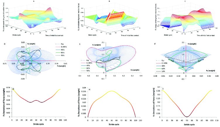
Figure 1: Schematic illustration of the observed spectrum for tIFC and GRF showing the relationship between tIFC and GRF in three directions (Fig.1A - C), together with tIFC and GRF resultant force in three planes (Fig.1D - F), compared with a typical tIFC and dispersion of force correspondence (Fig.1G - I).

Fig. 1D - F indicates that no matter what changes $t_{o}$ undergoes, GRF resultant forces in these three planes remain to be closed curves. This significantly compliments and confirms the dynamics behind Eq. (3), i.e., when the distribution of one foot’s GRF is determined and both feet’s GRFs remain the same, the momentum of COM always remains unaffected.

Fig. 1D - F also reveals the geometrical characteristics of the plane resultant force. On the transverse plane, when $t_{o}=0,T$, the gait becomes a jump and its frontal resultant force becomes a straight line. The resultant force changes into a symmetrical butterfly about $F_{x}$, which could imply a possible transformation at $t_{o}=\frac{1}{2}T$. On the sagittal plane, when $t_{o}=0,T$, the resultant force $F_{xz}$ forms the longest closed curve (the length of which is calculated by $\oint F_{xz}(t,t_{o})dF_{x}dF_{y}$) and more or less shortest at $t_{o}=\frac{1}{2}T$. On the frontal plane, when the resultant force develops into a straight line at $t_{o}=0,T$, the resultant force becomes a symmetrical butterfly about $F_{z}$ at $t_{o}=\frac{1}{2}T$.

Having developed the relationship between tIFC and GRF’s resultant force on three planes, we calculate the GRF dispersion in three directions using Eq. (4). To confirm the results beyond doubt, we identify the GRF dispersion by analyzing the effective plots shown in Fig. 1G - I. It is clear from the plots that at $t_{o}=\frac{1}{2}T$, $\sigma_{x}$ has its maximum value at the bottom region of ”W” shape, $\sigma_{y}$ has a global maxima and $\sigma_{z}$ a global minima. Using the numerical values, $min(\sigma_{x})=0.0695$, $max(\sigma_{x})=0.1319$, $min(\sigma_{y})=0.0000$, $max(\sigma_{y})=0.0355$, $min(\sigma_{z})=0.1086$ and $max(\sigma_{z})=0.9144$, of GRF dispersion obtained in this case study, we find that the largest differences between the maximal and minimal values are $0.0624$, $0.0355$ and $0.8058$, respectively. This means that the dominant effect to the global GRF is the longitudinal GRF. The minimal GRF dispersion on longitudinal direction occurs at $t_{o}=\frac{1}{2}T$. The analysis of the distribution of GRF in three directions indicates that when $t_{o}=\frac{1}{2}T$, the anteroposterior and longitudinal dispersions of GRF are almost the least and the mediolateral one is the largest. The closed curve shaped by the two components on the sagittal plane seems to be the shortest. The GRF resultant force on the transverse and sagittal plane is shown as symmetric butterfly.

Turning our attention towards the kinetic regularities, we plot the effect of tIFC on COM velocity in Fig. 2. We can see two platforms in Fig. 2A - C, which emerge at the two extremes of tIFC rated by percentage forming a concave region around tIFC whereas the velocity describes a convex region around tIFC. The COM velocity in the longitudinal direction indicates that tIFC entails the vertical velocity of COM to have a distribution of tIFC in the form of a saddle. In order to further understand the effect of tIFC exerting on the velocity of COM, we analyze the variations of the velocity of COM in three planes.

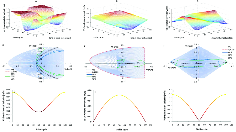
Figure 2: Effective plots showing relationship between tIFC and COM velocity in three directions (Fig.2A - C), tIFC and COM velocity in three planes (Fig.2D - F) and tIFC and dispersion of COM velocity (Fig.2G - I).

Looking at Fig. 2D - F, we notice that in the transverse plane, the direction of COM velocity is a straight line at $t_{o}=0$ and $T$ and the plane velocity becomes a symmetrical closed curve about $v_{x}$ axis at $t_{o}=\frac{1}{2}T$. In the sagittal plane the closed curve formed by the plane velocity is the longest (the length of the closed curve is calculated by $\oint v(t,t_{o})dv_{x}dv_{z}$) at $t_{o}=0,T$, and is shorter (not the shortest) at $t_{o}=0$ and $T$. In the frontal plane, when $t_{o}=0,T$, the velocity becomes a straight line and the resultant velocity becomes a symmetrical closed curve about $v_{z}$ axis at $t_{o}=\frac{1}{2}T$. Having obtained the estimated value of COM velocity, we are ready to set up the dispersion of relationship between tIFC and COM velocity (as shown in Fig. 2G - I) using Eq. (4). We notice that at $t_{o}=\frac{1}{2}T$, $\sigma_{x}$ and $\sigma_{y}$ have the global minima and $\sigma_{z}$ has the global maxima. The estimates, $min(\sigma_{x})=0.0541$, $max(\sigma_{x})=0.1652$, $min(\sigma_{y})=0.0000$, $max(\sigma_{y})=0.0510$, $min(\sigma_{z})=0.0549$ and $max(\sigma_{x})=1.3502$ in our case study, result in largest differences of maximal and minimal values of $0.1111$, $0.0510$, and $1.2953$ respectively. This means that the dominant effect upon COM velocity lies in the longitudinal and anteroposterior directions, where the dispersions have the minimal values at $t_{o}=\frac{1}{2}T$.

The kinematic regularity of the displacement of COM in three directions is shown in Fig. 3A - C. We see a geometric distribution of convex corners indicating that tIFC changes the position of COM in anteroposterior and mediolateral direction. The bimodal plot indicates the complexity of longitudinal direction exerted by tIFC to the position of COM. The estimated values of the COM displacement components are used to evaluate the values and directions of COM displacement in three planes. To further analyze the effect of tIFC upon the position of COM, we explore the changes of COM positions from three planes which are displayed in Fig. 3D - F.

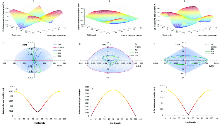
Figure 3: COM displacement as a function of tIFC. The directional and planer components are shown in Fig.3A - C and Fig.3D - F, respectively. Fig.3G - I shows the dispersion of COM displacement.

These effective plots show that in the transverse plane the COM displacement is a straight line at $t_{o}=0,T$. On the other hand a closed curve is formed by $s_{x}$ and $s_{y}$ and is symmetric about $s_{x}$ axis at $t_{o}=\frac{1}{2}T$. On the sagittal plane, when $t_{o}=0,T$, the closed curve shaped by the sagittal displacement is the longest (the length of the closed curve is calculated by $\oint s(t,t_{o})ds_{x}dy_{z}$); when $t_{o}=\frac{1}{2}T$, the curve is rather shorter (but not the shortest). On the frontal plane the frontal displacement becomes a straight line at $t_{o}=0,T$ and a symmetric closed curve about $s_{y}$ axis at $t_{o}=\frac{1}{2}T$.

Using the numerical values, $min(\sigma_{x})=0.0042$, $max(\sigma_{x})=0.0252$, $min(\sigma_{y})=0.0000$, $max(\sigma_{y})=0.0081$, $min(\sigma_{z})=0.0039$ and $max(\sigma_{z})=0.2147$, obtained in this case study, we find that of the GRF dispersion $\sigma_{x}$ and $\sigma_{y}$ have a global minima and $\sigma_{z}$ has a global maxima at around $t_{o}=\frac{1}{2}T$, again resulting in largest differences between the minimal and maximal values with a magnitude of the order $0.0210$, $0.0081$ and $0.2108$, respectively. This implies that the greatest effect to COM displacement comes from components on longitudinal and anteroposterior directions while the minimal dispersion of displacement on the longitudinal and anteroposterior direction emerges at $t_{o}=\frac{1}{2}T$ (See Fig. 3G - I).

Accordingly, at $t_{o}=\frac{1}{2}T$, COM velocity in relative motion presents its symmetric closed curve in transverse and frontal plane and the curve length in the sagittal plane is approximately the minimal. In a stride cycle, the dispersion of COM velocity in relative motion has the global minima on the anteroposterior and longitudinal direction while the global maximal value on the mediolateral direction. The effect of tIFC upon the COM velocity and displacement does not depend on gait velocity, cadence or stride length whereas the effect of the tIFC upon COM acceleration is in accordance with the effect it exerts upon the GRF. The COM acceleration and GRF show more or less identical behaviour. Fig. 4A - C demonstrate the effect of tIFC upon three components of GRF, COM velocity and COM displacement on three direction. As is clear from Fig. 4D - F that at half stride cycle ($t=T/2$), the dispersion of GRF and COM kinematics are minimum. In comparison to GRF and COM velocity, the COM displacement shows a sharp dip with least minimum.

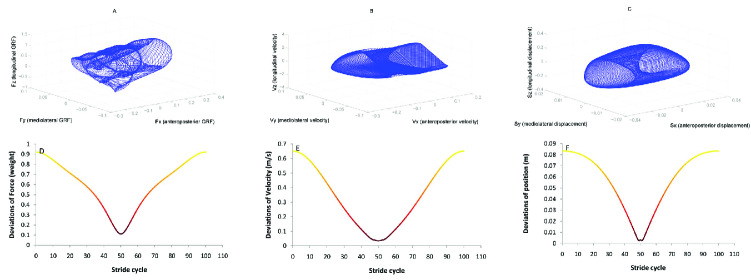
Figure 4: Relationship between tIFC and dispersion of force.

3.2 Anteroposterior, Mediolateral and longitudinal average kinetic energies

Finally, we show the COM kinetic energies as a function of stride cycle in anteroposterior, mediolateral and longitudinal channels in Fig. 5A - C, together with corresponding transverse, sagittal and frontal energies in three planes (Fig. 5D - F). Fig. 5G - I indicates that tIFC makes COM average kinetic energy the global minima on anteroposterior and mediolateral direction while that on the mediolateral direction a global maxima at $t_{o}=\frac{1}{2}T$. Comparing the relationship between the tIFC’s velocity of COM and the position of COM, tIFC contributes a symmetric distribution of kinetic energy of COM. Since $min(E_{x}(t,t_{o}))>max(E_{y}(t,t_{o}))$ and $max(E_{y}(t,t_{o}))<min(E_{z}(t,t_{o}))$, the anteroposterior and longitudinal average kinetic energies determine the COM average kinetic energy.

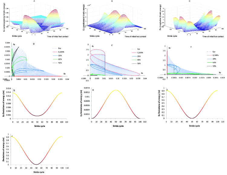
Figure 5: Relationship between tIFC and kinetic energy. (Fig.5A - C tIFC and COM kinetic energy in three directions; Fig.5D - F -tIFC and COM kinetic energy in three planes; Fig.5G - I - tIFC and average kinetic energy. )

when tIFC falls at the $20\%,50\%,60\%$ and $100\%$ of a stride cycle, the kinetic energy of COM in three planes varies rather considerably. On the transverse and frontal planes, the effect is similar whereas the sagittal plane undergoes a non-trivial change. We apply the dispersion of kinetic energy of COM to evaluate this effect. We notice, from Fig. 5J, that COM average kinetic energy is minimum at $t_{o}=\frac{1}{2}T$, which implies a minima for the COM mechanical energy consumption and signatures the physical significance of gait.

3.3 Least-action principle in gait

The intriguing question that arises from the above discussion if there is a symmetry or a physical principle that is hidden in the phenomenon that makes the COM kinetic energy to reach its extremum at $t_{o}=\frac{1}{2}T$. In order to explore this issue, we pursue the technique of optimizing the dispersion objective function [18]

$$\sum^{T}_{1}(f(t)+f(t+t_{o})-\overline{f}(t_{o}))^{2}=\sum^{T}_{1}f(t)^{2}+\sum^{T}_{1}f(t+t_{o})^{2}$$

$$+2\sum^{T}_{1}f(t)f(t+t_{o})-2\sum^{T}_{1}(f(t)+f(t+t_{o}))+(\overline{f}(t_{o}))^{2}\sum^{T}_{1}1$$ (11)

The action of GRF and gravity are the reasons for human COM motion changes. Let’s first analyze the GRF. The average value of the resultant force in the anteroposterior and mediolateral direction $\bar{F}_{x}(t_{o})$ and $\bar{F}_{y}(t_{o})$ is zero and in the longitudinal direction $\bar{F}_{z}(t_{o})$ is one (when the weight has been normalized). Therefore, for a known gait, $\sum^{T}_{1}(F_{x}(t))^{2},\sum^{T}_{1}(F_{y}(t))^{2},\sum^{T}_{1}(F_{z}(t))^{2},\sum^{T}_{1}(F_{x}(t+t_{o}))^{2},\sum^{T}_{1}(F_{y}(t+t_{o}))^{2}$ and $\sum^{T}_{1}(F_{z}(t+t_{o}))^{2}$ are all constants and Eq. (11) simplifies the dispersion optimization to

$$\min\psi_{F_{x}}(t_{0}) = \sum_{1}^{T}F_{x}(t)F_{x}(t+t_{o})$$

$$\max\psi_{F_{y}}(t_{0}) = \sum_{1}^{T}F_{y}(t)F_{y}(t+t_{o})$$

$$\min\psi_{F_{z}}(t_{0}) = \sum_{1}^{T}F_{z}(t)F_{z}(t+t_{o}).$$ (12)

To find a solution of the optimization problem, we need to set up a function of GRF that changes with time in three directions. It seems that the pulse periodic GRF fits the criteria and hence we use segment trigonometric functions

$$F_{x}(t)=a\sin(2\pi\frac{t}{T_{s}}),\hskip 14.22636ptF_{y}(t)=b\sin(\pi\frac{t}{T_{s}})\hskip 14.22636ptF_{z}(t)=c\sin(\pi\frac{t}{T_{s}}),$$

where $a,b,c$ stand for the GRF after normalization in three directions and $T_{s}$ is the stance time. For a small enough test frequency, the above equation transforms to

$$\min\psi_{F_{x}}(t_{0}) = A\int^{T_{s}}_{0}\sin(2\pi\frac{t}{T_{s}})\sin(2\pi\frac{t+t_{o}}{T_{s}})dt$$

$$\max\psi_{F_{y}}(t_{0}) = -B\int^{T_{s}}_{0}\sin(\pi\frac{t}{T_{s}})\sin(\pi\frac{t+t_{o}}{T_{s}})dt$$

$$\min\psi_{F_{z}}(t_{0}) = C\int^{T_{s}}_{0}\sin(\pi\frac{t}{T_{s}})\sin(\pi\frac{t+t_{o}}{T_{s}})dt.$$ (13)

Let’s take longitudinal GRF in Eq. (3.3) as an example. In order to get the antiderivative of the integrand of integral variable $t$, we detach $t$ and $t_{o}$ of trigonometric function to obtain

$$\int^{T_{s}}_{0}\sin(\frac{t}{T_{s}}\pi)\sin(\frac{t+t_{o}}{T_{s}}\pi)dt=\int^{T_{s}}_{0}(\sin^{2}(\frac{t\pi}{T_{s}})\cos(\frac{t\pi}{T_{s}})$$

$$+\sin(\frac{t\pi}{T_{s}})\cos(\frac{t\pi}{T_{s}})\sin(\frac{t_{o}\pi}{T_{s}}))dt,$$ (14)

Now we can transform Eq. (3.3) into the integral of integral variable $t$ while regarding the GRF as segment function. The transformation reduces the pulse periodic GRF functions into three piecewise functions at three intervals: $[0,T_{w}]$, $[T_{w},T_{s}]$ and $[T_{s},T]$ which, to the confirmed GRF, $a,b,c$ are constants and $A,B,C$ (related to $a,b,c$) are also constants, yields the following form of longitudinal GRF:

$$\min\psi_{F_{z}}(t_{o})=C\cases{\frac{1}{2}\sin(\pi\frac{t_{o}}{T_{s}})-(\frac{t_{o}-T_{s}}{2T_{s}}\pi)\cos(\pi\frac{t_{o}}{T_{s}})\\ 0\leq t_{o}\leq T_{w}\\ \frac{1}{2}\sin(\pi\frac{t_{o}}{T_{s}})-(\frac{t_{o}-T_{s}}{2T_{s}}\pi)\cos(\pi\frac{t_{o}}{T_{s}})\\ +\frac{1}{2}\sin(\frac{t_{o}-T_{w}}{T_{s}}\pi)-(\frac{t_{o}-T_{w}}{2T_{s}}\pi)\cos(\frac{t_{o}-T_{w}}{T_{s}})\\ T_{w}\leq t_{o}\leq T_{s}\\ \frac{1}{2}\sin(\frac{t_{o}-T_{w}}{T_{s}}\pi)-(\frac{t_{o}-T_{w}}{2T_{s}}\pi)\cos(\frac{t_{o}-T_{w}}{T_{s}}\pi)\\ T_{s}\leq t_{o}\leq T\\ }$$

The contribution $(\frac{t_{o}-T_{s}}{2T_{s}}\pi)\sin(\pi\frac{t_{o}}{T_{s}})=0$ in the interval $[0,T_{w}]$, thus giving the $t_{o}=0$, which in turn yield (from Eq. (3.3)) a maxima ($=\frac{C\pi}{2}$). On the other hand, the contribution $(\frac{t_{o}-T_{s}}{2T_{s}}\pi)\sin(\pi\frac{t_{o}}{T_{s}})+(\frac{t_{o}-T_{w}}{2T_{s}}\pi)\sin(\pi\frac{t_{o}-T_{w}}{T_{s}})=0$ in $[T_{w},T_{s}]$ giving the solution $T_{s}-t_{o}=t_{o}-T_{w}$ which yields $C(\cos(\frac{T_{w}}{2T_{s}}\pi)-(\frac{T_{s}-T_{w}}{2T_{s}}\pi)\sin(\frac{T_{w}}{2T_{s}}\pi))$ (a minima). Similarly, we obtain a maximum value $\frac{C\pi}{2}$ in $[T_{s},T]$.

Following the above procedure, it is easy to verify (from Eq. 3.3) that at $t_{o}=T/2$ the dispersion of GRF in the anteroposterior direction attains a minima of $A((\frac{T_{w}-T_{s}}{T_{s}}\pi)\cos(\frac{T_{w}}{T_{s}}\pi)-\sin(\frac{T_{w}}{T_{s}}\pi))$ and a maxima of $B((\frac{T_{s}-T_{w}}{2T_{s}}\pi)\sin(\frac{T_{w}}{2T_{s}}\pi)-\cos(\frac{T_{w}}{2T_{s}}\pi))$. in the mediolateral direction. Since, in gait, $A>B>C$, the sum of dispersions in three directions is minimal at $t_{o}=\frac{1}{2}T$. This confirms our results shown in Figs. 4D - F and 5J. Similarly, the dispersion of COM acceleration, dispersion of COM velocity and the COM mechanical energy consumption are all the minimal at $t_{o}=\frac{1}{2}T$. This phenomenon is independent of the physiological factors such as height, weight and gait parameters [18].

4 Conclusion

In periodic motion, the foot’s stance and swing substitute one another such that one foot always remains in stance. This allows the human body to be acted by the periodical GRF, which is related not only to the foot’s movement style, but also to the substitution style of one foot with another. Following the biped movement style in normal gaits and the similar traits of GRF, we have been able to study the effect of tIFC upon the human COM dynamic characteristics based on the assumption that both feet’s GRFs are the same in the same phase. Our results suggest that when tIFC falls in the middle of the other foot’s stride cycle, the COM kinematics and dispersions of GRF acted on COM are the minimal, which has entailed the minimal average MEC of muscles. Our analysis suggests that it falls into the category of least-action principle and is consistent with the phenomenon that exists in normal gaits [18].

Based upon the least-action principle, we have observed that tIFC has caused the GRF and the COM regularities to form a closed-curve on the transverse and frontal plane, which might present a new method for gait evaluation. We advocate the use of this method to uncover and speed up the diagnosis simply by measuring the GRF for the patients with foot injuries or arthritis (for such patients, the model for these quantities is not symmetric [27]). Meanwhile, the patients need only walk a few steps in their normal gait, their COM dynamic characteristics will be acquired easily and more accurately. This is exactly what the clinic diagnosis is looking for. In addition to the human gait’s adaptation to natural environment [25, 28], the evolution of gait is the result of its observation of least-action principle. We believe that precise measurements of the variations of shear stress in natural gaits (bare-footed) shall profoundly enriched the content of least-action principle [29]. A further study of least-action principle will be significant to the domains such as sport rehabilitation, biometric identification [30, 31] and control of biped robot gaits [32, 33, 34].

References

References

- [1] Mitoma H, Hayashi R, Yanagisawa N and Tsukagoshi H 2000 J. Neurol. Sci. 174 22
- [2] Kim C M and Eng J J 2003 Gait Posture 18 23
- [3] Vaughan C, Davis B, and O’Connor J 1999 Dynamics of Human Gait, second ed., Kiboho, Cape Town
- [4] Yang N F, Wang R C, Jin D w, Dong H, Huang C H, Zhang M 2001 Chinese Journal of Rehabilitation Medicine 16 336 (in Chinese)
- [5] Kondraske G 1994 Proceedings of the 16th Annual International Conference of the IEEE Engineering in Medicine and Biology Society, Baltimore, USA 1 307
- [6] Titianova E B and Tarkka I M 1995 J. Rehabil. Res. Dev. 32 236
- [7] Liu Y B, Yan N and Yun X P 2000 Modern Rehabilitation 4 28 (in Chinese)
- [8] Biswasa A, Lemaire E and Kofman J 2008 J. Biomech. 41 1574
- [9] Wall J C and Turnbull G I 1986 Arch. Phys. Med. Rehabil. 67 550
- [10] Liu Y B, and Yan N 1996 Chinese Journal of Rehabilitation Theory and Pactice 2 154 (in Chinese)
- [11] Sadeghi H, Allard P, Prince F and Labelle H 2000 Gait Posture 12, 34
- [12] Wang R C, Zhang M Q, Hua C, Deng X N, Yang N H and Jin D W2005 J. Tsinghua Univ. 45, 190 (in Chinese)
- [13] Yang Y Y, Wang R C, Hao Z X, Jin D W, Zhang H 2005 J. Biomed. Eng. 45 1100 (in Chinese)
- [14] Kokshenev V B 2004 Physical Review Letters 93 208101
- [15] Gutierrez-Farewik E M, Bartonek A and Saraste H 2006 Hum. Movment Sci. 25 238
- [16] Winiarski S and Rutkowska-Kucharska A 2009 Acta of Bioengineering and Biomechanics 11 53
- [17] Murray M 1967 Am. J. Phys. Med. 46 290
- [18] Fan Y F, Loan M, Fan Y B, Li Z Y and Luo D L 2009 Europhys. Lett. 87 58003
- [19] Gard S A, Miff S C and Kuo A D 2004 Hum. Movment Sci. 22 597
- [20] Fan Y F, Li Z Y and Lv C S 2008 Proc. SPIE 7128 71280I
- [21] Ren L, Jones R K and Howard D 2008 J. Biomech. 41 2750
- [22] Anderson F C and Pandy M G 2001 J. Biomech. Eng-T ASME 123 381
- [23] Chau T 2001 Gait Posture 13 49
- [24] Marion J 1970 Classical Dynamics of Particles and System (Academic, New York)
- [25] Jenkins F A 1972 Science 178 877
- [26] Srinivasan M and Ruina A 2006 Nature 439 72
- [27] Kfc 2009 Technology Review http://www.technologyreview.com/blog/arxiv/23569
- [28] Richmond B G and Jungers W L 2008 Science 319 1662
- [29] LIU D W 2007 Science Technology and Engineering 7 2319 (in Chinese)
- [30] Boulgouris N V, Hatzinakos D and Plataniotis K N 2005 IEEE Signal Proc. Mag. 22 78
- [31] Nixon M S and Carter J N P. IEEE 94 2013
- [32] Collins S H, Wisse M and Ruina A 2001 Int. J. Robot Res. 20 607
- [33] Collins S, Ruina A, Tedrake R and Wisse M 2005 Science 307 1082
- [34] Ohgane K and Ueda K I 2008 Phys. Rev. E 77 051915