Geometric phase as a determinant of a qubit–environment coupling

Abstract

We investigate the qubit geometric phase and its properties in dependence on the mechanism for decoherence of a qubit weakly coupled to its environment. We consider two sources of decoherence: dephasing coupling (without exchange of energy with environment) and dissipative coupling (with exchange of energy). Reduced dynamics of the qubit is studied in terms of the rigorous Davies Markovian quantum master equation, both at zero and non–zero temperature. For pure dephasing coupling, the geometric phase varies monotonically with respect to the polar angle (in the Bloch sphere representation) parameterizing an initial state of the qubit. Moreover, it is antisymmetric about some points on the geometric phase-polar angle plane. This is in distinct contrast to the case of dissipative coupling for which the variation of the geometric phase with respect to the polar angle typically is non-monotonic, displaying local extrema and is not antisymmetric. Sensitivity of the geometric phase to details of the decoherence source can make it a tool for testing the nature of the qubit–environment interaction.

1 Introduction

One of the key obstructions of an effective implementation of quantum algorithms is related to the ubiquitous problem of decoherence in real quantum objects nielsen . Quantum decoherence is generic as it results from the imperfect isolation of the quantum system from its environment. Decoherence can be diminished under very special conditions such as e.g. the presence of the decoherence free subspaces decohfree or via the application of tailored, external control schemes kohler . A promising novel direction in quantum information relates to so called holonomic or topological quantum computations zanardi ; topol allowing for a substantial reduction of decoherence hqc ; aqc . The essence of this method consists in encoding the information in the holonomy related to the geometric phase of the quantum evolution berry . The geometric phase can be expressed as a path integral and via the Stokes theorem, can be converted into a surface integral. Therefore, it behaves like a geometric area. A quantity like an area is less dependent on the details of time evolution and therefore is less affected by changes of environmental conditions or an imperfect control, and hence, is typically more robust. This is the key attribute that makes geometric phases attractive for the implementations of fault-tolerant quantum computation. Some suggestions have been presented to realize this objective, e.g. in NMR experiments hqc , ion traps duan , neutral atoms in cavity QED recati , quantum dots yellow or Josephson junction devices falci . The performance of holonomic quantum gates under various conditions has been studied recently parodi .

The quantum evolution in the presence of decoherence is generically non–unitary. Therefore, the notion of geometric phase needs to be extended. There are several extensions of the geometric phase concept for systems which are either in a mixed state or/and undergo a non–unitary evolution. The first attempt towards this goal is given in armin , being rather of mathematical character. The other are based on quantum trajectories traj , quantum interferometry sjuk1 and the state purification (kinematic approach) muki ; sjuk2 . For non–unitary quantum evolution there is no commonly accepted scheme of defining the geometric phase in open quantum systems nowe . Here we use the approach based on state purification as proposed in Ref. sjuk2 . This so defined geometric phase has been extensively studied in various contexts ph1 ; ph2 . One of the appealing ’advantages’ of studying the phase defined in sjuk2 is that it can be measured with a carefully prepared interferometric experiment sjuk1 ; sjuk2 . Our reasoning is thus guided by its potential for experimental implementation.

There is no unique method of describing the time evolution of open quantum systems and there are several schemes to treat such systems which however typically give rise to non-equivalent dynamics chaos ; ali1 . One scheme consists in the derivation of a reduced system dynamics, via tracing over the degrees of freedom of the environment. Except some few exactly solvable models chaos ; ali it is not clear how to relate the reduced dynamics to the microscopically first principles dynamics based upon the Hamiltonian structure of quantum dynamics chaos ; romero . The exactly solvable model of pure dephasing has been applied for studying quantum channels anizfid or in exploring the dynamics of quantum entanglement abel . Despite its simplicity the highly non–trivial properties of geometric phase of qubits has also been discussed myfaz . One of the most successful examples of constructing reduced dynamics is the Davies approximation scheme davies . Within this approach, starting with the general ’system–bath–interaction’ Hamiltonian, one obtains, in a mathematically rigorous way, a Markovian master equation form of a quantum system weakly coupled to the environment which preserves positivity and yields the correct equilibrium Gibbs state spohn . This approach has been applied to various problems of statistical physics, quantum optics, solid state physics and quantum information, e. g. for studying entanglement dynamics in bipartite systems lendi .

In this paper we apply the Davies master equation to study the geometric phase of the qubit coupled to the bosonic bath. Various families of a coupling and different coupling strength are shown to result in a qualitative and quantitative modification of the geometric phase. This behavior could suggest a method to resolve the nature of the qubit-bath coupling: In particular, the dephasing coupling presents not only a mere theoretical construction but can be realized in experiments within tailored regimes devoret . In order to keep this study self–contained, we briefly review the notion of the geometric phase for a non–unitarily evolving qubit and then present the qubit master equation derived from the Davies theory.

2 Geometric phase

Generally, the time evolution of the qubit reduced density matrix $\rho(t)$ is neither unitary nor Markovian chaos ; romero . It is constructed as the mapping

$$\rho(t)=\Lambda(t,t_{0})\rho(t_{0})$$ (1)

obeying some properties depending on the specific circumstances and approximations such as e.g. the celebrated complete positivity condition alickilendi . In order to exploit the approach to the geometric phase based on state purification sjuk2 we have to present the reduced density matrix (1) in the spectral-decomposition form

$$\rho(t)=\sum_{i=1}^{2}p_{i}(t)|w_{i}(t)\rangle\langle w_{i}(t)|,$$ (2)

where $p_{i}(t)$ and $|w_{i}(t)\rangle$ are the eigenvalues and the eigenvectors of the matrix $\rho(t)$, respectively. The geometric phase $\Phi(t)$ associated with such an evolution is defined as follows sjuk2 :

$$\Phi(t) = \arg\left[\sum_{i=1}^{2}[p_{i}(0)p_{i}(t)]^{1/2}\langle w_{i}(0)|w_{i}(t)\rangle\right.$$ (3)

$$\left.\times\exp(-\int_{0}^{t}\langle w_{i}(s)|\dot{w}_{i}(s)\rangle ds)\right],$$

where $\arg$ denotes the argument of the complex number, $\langle w_{i}|w_{j}\rangle$ is a scalar product and the dot indicates the derivative with respect to time $s$. For convenience, we assume the initial time being $t_{0}=0$. For the sake of completeness we sketch here, following Ref. sjuk2 , the derivation of Eq.(3). The mixed state defined by the density matrix (2) can be lifted to a pure state $|\Psi(t)\rangle$ in a larger Hilbert space, i.e.,

$$|\Psi(t)\rangle=\sum_{i=1}^{2}\sqrt{p_{i}(t)}|w_{i}(t)\rangle\otimes|a_{i}\rangle,$$ (4)

where the vectors $|a_{i}\rangle$ span the Hilbert space of an arbitrary ancilla. This is known as a purification of the density matrix $\rho(t)$ in the sense that $\rho(t)$ is a partial trace of the density matrix $|\Psi(t)\rangle\langle\Psi(t)|$ over the ancilla Hilbert space. With the time evolution of the purified system one can associate the ’Pancharatnam’ relative phase

$$\alpha(t)=\arg\langle\Psi(0)|\Psi(t)\rangle$$ (5)

which contains both the gauge–dependent part (a dynamical phase) and a gauge–independent part. The central result of sjuk2 is to extract from Eq.(5), by a proper choice of the ’parallel transport condition’, the purification–independent part which can be termed a geometric phase because it is gauge invariant and reduces to the known results in the limit of an unitary evolution anandan ; chruscinski . The final result is then given by Eq. (3).

As mentioned in the Introduction, this phase – contrary to other attempts of extending the notion of geometric phase for a non–unitary evolving quantum system – has a direct physical meaning as it can be measured via interferometric experiments sjuk2 , i.e. one can construct the purification of the quantum system such that the relative phase (5) reduces to the geometric phase (3) after suitably defined ’compensating unitary’ cutting of the dynamical part of the relative phase sjuk2 .

3 Weak coupling regime of qubit reduced dynamics

The evolution operator $\Lambda(t,t_{0})$ defined by equation (1) or its infinitesimal generator $\mathcal{L}$ defined by the equation

$$\frac{d}{dt}\rho(t)=\mathcal{L}\{\rho(t)\}$$ (6)

can be obtained in a few cases only; namely for stylized, exactly solvable models or in the limiting regimes such as the weak coupling limit or the singular coupling limit alickilendi . We consider a qubit coupled to a bosonic environment at temperature $T$. The Hamiltonian of such a system is chosen in the form chaos :

$$H = H_{Q}\otimes\mathcal{I}+\mathcal{I}\otimes H_{B}+H_{I}\otimes V_{B},$$ (7)

$$H_{B} = \int_{0}^{\infty}E(k)a^{\dagger}(k)a(k)dk,$$ (8)

$$V_{B} = \int_{0}^{\infty}g(k)[a^{\dagger}(k)+a(k)]dk.$$ (9)

The operators $a^{\dagger}(k)$ and $a(k)$ denote the creation and annihilation boson operators, respectively. The qubit Hamiltonian and the interaction are assumed to take the form

$$H_{Q} = \frac{\varepsilon}{2}\sigma_{z},\,\,\,\,\,\,H_{I}=\hbar\mu_{x}\sigma_{x}+\hbar\mu_{z}\sigma_{z},$$ (10)

where $\sigma_{i}$ are the Pauli operators, $\varepsilon$ is the qubit energy splitting and the dimensionless parameters $\mu_{x}$ and $\mu_{z}$ are coupling constants. Let us remark that if $\mu_{x}\equiv 0$ the qubit energy operator $H_{Q}$ is an integral of motion, i.e. it commutes with the total Hamiltonian $H$ leaving the expectation value of the corresponding energy observable unchanged. This situation defines the well known exactly solvable model of pure dephasing ali . A non-vanishing $\mu_{x}$ is then characteristic for exchange of energy and related dissipation processes.

For an uncorrelated initial state $\rho(0)\otimes w(\beta)$ taken as a product of an arbitrary qubit density matrix $\rho(0)$ and the equilibrium Gibbs state of the environment $w(\beta)=\exp(-\beta H_{B})/\mbox{Tr}[\exp(-\beta H_{B})]$ with $\beta=1/k_{B}T$ ($k_{B}$ is the Boltzmann constant), the Davies approximation for the Markovian kernel yields the following Markovian master equation davies ; spohn

$$\frac{d}{dt}\rho(t)=\mathcal{L}_{H}\{\rho(t)\}+\mathcal{L}_{R}\{\rho(t)\},$$ (11)

where the ’conservative’ and ’dissipative’ parts read as follows

$$\mathcal{L}_{H}\{\rho(t)\}=-\frac{i}{\hbar}[(H_{Q}+\sum_{k,l=-1}^{1}\hbar s(\Omega_{kl})A^{\dagger}_{kl}A_{kl}),\rho(t)],$$ (12)

$$\mathcal{L}_{R}\{\rho(t)\} = \frac{1}{2}\sum_{k,l=-1}^{1}c(\Omega_{kl})$$ (13)

$$\times \left([A_{kl}\rho(t),A_{kl}^{\dagger}]+[A_{kl},\rho(t)A_{kl}^{\dagger}]\right),$$

where, see in Refs. alickilendi ; lendi ,

$$A_{kl}=\mathcal{P}_{k}H_{I}\mathcal{P}_{l},\quad\mathcal{P}_{\pm 1}=|\pm 1\rangle\langle\pm 1|,$$

$$\Omega_{kl}=(\lambda_{k}-\lambda_{l})/\hbar,\quad\lambda_{\pm 1}=\pm\varepsilon/2.$$ (14)

The states $|1\rangle$ and $|-1\rangle$ denote the excited state and ground state of the qubit, respectively. The quantity $c(\omega)$ is the Fourier transform of the autocorrelation function of the bath operator $V_{B}$ calculated in the Gibbs state $w(\beta)$ of the bath, namely,

$$c(\omega)=\int_{-\infty}^{\infty}\mbox{e}^{-i\omega t}\,\mbox{Tr}[w(\beta)V_{B}\mbox{e}^{itH_{B}/\hbar}V_{B}\mbox{e}^{-itH_{B}/\hbar}]dt$$ (15)

and its Hilbert transform defines the function $s(\omega)$ in the following way

$$s(\omega)=\frac{\mbox{P}}{2\pi}\int_{-\infty}^{\infty}\frac{c(x)}{x-\omega}dx,$$ (16)

where P indicates the Cauchy principal value of the integral.

In order to treat the complex qubit–environment interaction encoded in $g(k)$ in (9) it is convenient to introduce the spectral density

$$D(\omega)=\int dk|g(k)|^{2}\delta(\omega(k)-\omega).$$ (17)

We further limit our consideration to the strictly Ohmic environment for which this spectral density is linear with respect to $\omega$ for small frequencies and exhibits an exponential cut-off frequency $\omega_{c}$, thereby exhibiting no non-physical ultraviolet divergences. Explicitly, this spectral density reads

$$D(\omega)=\frac{\alpha}{2}\omega\exp(-\omega/\omega_{c}),$$ (18)

where the dimensionless parameter $\alpha$ characterizes the strength of the environmental influence on the qubit. Within this choice alickilendi ; lendi

$$c(\omega)=\frac{\pi\alpha}{2}\left(|\omega|\frac{\exp(\beta\hbar|\omega|)+1}{\exp(\beta\hbar|\omega|)-1}+\omega\right)\exp(-|\omega|/\omega_{c})$$ (19)

and $s(\omega)$ is determined via the relation in (16).

In principle one can solve Eq. (11) using the Bloch vector formalism to obtain the coupled evolution equations for mean values $\langle\sigma_{k}(t)\rangle,k=x,y,z$ to obtain the reduced density matrix as $\rho(t)=(1/2)[1+\langle\sigma_{x}(t)\rangle\sigma_{x}+\langle\sigma_{y}(t)\rangle\sigma_{y}+\langle\sigma_{z}(t)\rangle\sigma_{z}]$. This form allows to extract the spectral decomposition (2) and the phase $\Phi(t)$. Such an explicit form of the geometric phase result is, however, rather cumbersome without exhibiting much physical insight. We thus refrain from presenting such analytical details, but present here the full analysis of the geometric phase by numerical means.

4 Analysis of geometric phase

From Eqs (1)-(3) it follows that in order to determine the geometric phase at arbitrary time $t>0$, we must specify the initial state of the qubit. We consider the following class of initial states

$$|\theta\rangle=\cos(\theta/2)|1\rangle+\sin(\theta/2)|-1\rangle,$$ (20)

where $\theta$ is the polar angle in the Bloch sphere representation. The corresponding initial statistical operator $\rho(0)$ takes the form

$$\rho(0)=|\theta\rangle\langle\theta|.$$ (21)

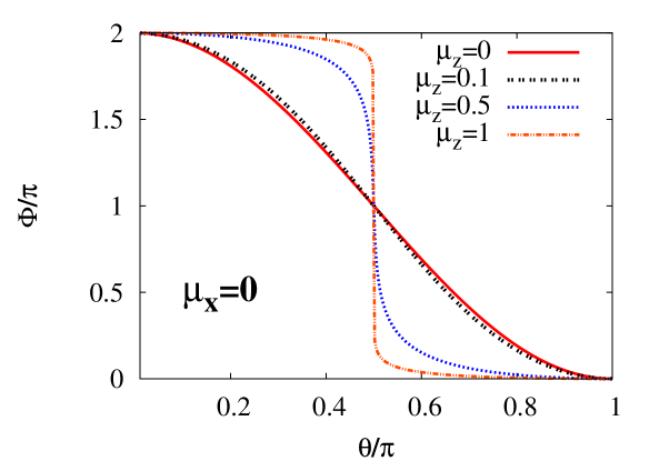
Figure 1: (Color online) Dependence of the geometric phase $\Phi=\Phi({\cal T})$ on the initial state of the qubit which is parameterized by the angle $\theta$ on the Bloch sphere. The qubit is coupled to a purely dephasing Ohmic environment, i.e. $\mu_{x}=0$ in (10). The remaining parameters are: $\alpha=10^{-2}$, $\hbar\omega_{c}/\varepsilon=10^{2}$ and $T=0$.

One of the eigenvalues of this operator is zero, say $p_{2}(0)=0$ in Eq. (3), and it does not contribute to the geometric phase. This simplifies Eq. (3) in that only one term of the sum survives. The evolution of the freely evolving qubit, with $\mu_{x}=\mu_{z}=0$ in (10), is cyclic with the time-period ${\cal T}=2\pi\hbar/\varepsilon$ and it acquires the geometric phase chruscinski

$$\Phi_{0}=\pi[1+\cos(\theta)],\quad\mbox{mod}(2\pi),$$ (22)

which can serve as a reference for studying the influence of the environment. In the case of a coupling to an environment, the evolution of the qubit is not cyclic any longer. However, below we consider the phase $\Phi=\Phi({\cal T})$ after the time ${\cal T}=2\pi\hbar/\varepsilon$ in order to study the role of coupling to the environment and for comparison with (22).

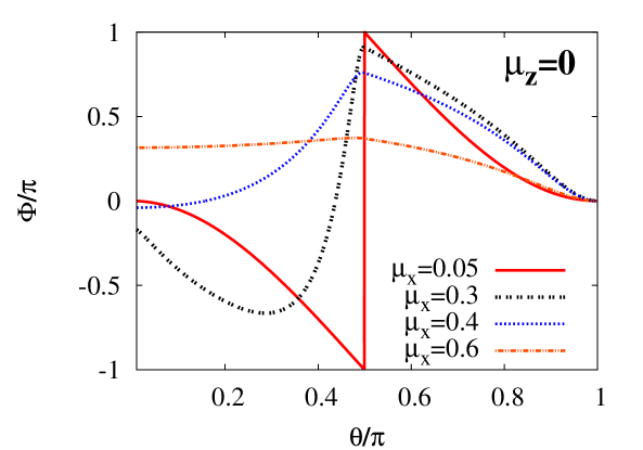
Figure 2: (Color online) Geometric phase $\Phi=\Phi({\cal T})$ vs. initial polar angle $\theta$ for selected values of the dissipative qubit - Ohmic environment coupling strength $\mu_{x}$. The dephasing coupling strength is set at $\mu_{z}=0$ in (10), and the remaining parameters are the same as in Fig. 1.

The simplest situation occurs for pure dephasing; i.e. when $\mu_{x}=0$ so that the qubit energy does not change. The results presented in Fig. 1 show that the geometric phase plotted as a function of the initial state of the qubit (i.e. as a function of the parameter $\theta$ in Eq. (20)) approaches zero (modulo $2\pi$) with increasing coupling strength $\mu_{z}$. We observe that it varies drastically in the regime near $\theta=\pi/2$ and varies weakly outside this region. Moreover, the phase vanishes for $\theta\to 0$ (i.e. for the initially excited state $|1\rangle$ ) and $\theta\to\pi$ (i.e. for the ground state $|-1\rangle$ ). This finding corroborates the results for the phase in the exactly solvable model of pure dephasing with arbitrary (not only weak) coupling myfaz . For the presentation as in Fig. 1, we note that the function $\Phi\left(\theta\right)$ is antisymmetric about the point $\{\theta,\Phi\}=\{\pi/2,\pi\}$, i.e. the relation

$$\Phi\left(\frac{\pi}{2}+\theta\right)=2\pi-\Phi\left(\frac{\pi}{2}-\theta\right)\quad\mbox{for}\quad\theta\in[0,\pi/2]$$ (23)

holds. It can be interpreted as a rotation symmetry around the point $\{\theta,\Phi\}=\{\pi/2,\pi\}$.

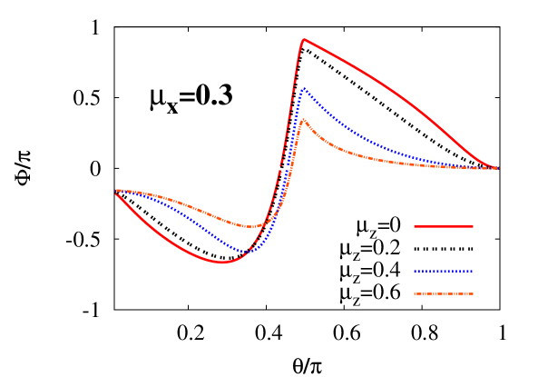
Figure 3: (Color online) Role of a qubit-environment coupling on the geometric phase $\Phi=\Phi({\cal T})$ vs. initial state preparation $\theta$ for a qubit that is coupled to an Ohmic environment. The dissipative coupling strength is set at $\mu_{x}=0.3$. The influence of dephasing is depicted for four different coupling strengths $\mu_{z}$. The remaining parameters are the same as in Fig. 1.

A most intriguing behavior on the role of the environment emerges when $\mu_{x}\neq 0$; i.e. when the qubit–environment interaction is allowed to exchange energy with the qubit system. The results depicted in Fig. 2 show the qualitative changes in the geometric phase properties for increasing dissipation coupling strength $\mu_{x}$ as a function of the polar angle $\theta$. Note that the geometric phase $\Phi$ in Fig. 2 is plotted differently from Fig. 1 with $\Phi/\pi$ varying within the interval $(-1,1)$. We have decided to make this change in order to avoid confusing jump-like behavior of $\Phi(\theta)$ in vicinity of the polar angle $\theta=\pi/2$. E. g. the curve corresponding to the case $\mu_{x}=0.05$ in Fig. 2 is very similar to the curve corresponding to the case $\mu_{z}=0.5$ in Fig. 1. However, presented in the $\Phi/\pi\in(-1,1)$ interval it exhibits jump-like behavior which is an artefact of the way the plot is done. Let us recall again here that the phase $\Phi$ is defined modulo $2\pi$.

For small values of $\mu_{x}$, the geometric phase is close to that for the isolated qubit, cf. $\mu_{x}=0.05$ in Fig. 2 when compared with Fig. 1 but with $\Phi$ varying there $\Phi/\pi\in(0,2)$. When $\mu_{x}$ increases the function $\Phi(\theta)$ exhibits a local maximum and minimum, see the case $\mu_{x}=0.3$ in Fig. 2. For larger value of the coupling strength $\mu_{x}$ (the case $\mu_{x}=0.4$ ) the geometric phase is an increasing function of the polar angle $\theta$ till to the value $\theta=\pi/2$ reaching a local maximum. Next, it decreases as $\theta\to\pi$. In comparison to the dephasing coupling, in this case we can find at least three distinguishing features of the geometric phase. Firstly, we note breaking of antisymmetry of $\Phi(\theta)$, being in distinct contrast to the case of pure dephasing ($\mu_{x}=0$), cf. Fig. 1. Secondly, the dependence of the phase on the initial state parameterized by $\theta$ is non-monotonic, exhibiting a local maximum and a minimum. Thirdly, the geometric phase $\Phi$ vanishes for $\theta\to\pi$ (i.e. for the ground state) but not necessary so for $\theta\to 0$ (i.e. for the excited state).

One can observe that for a fixed $\mu_{x}$, the dephasing process controlled by $\mu_{z}$ does not change the qualitative properties of the geometric phase $\Phi$, see Figs. 1 and 3. Pure dephasing affects only the off–diagonal elements of the density matrix, becoming closer to the maximally mixed qubit state. The geometric phase in a quantum evolution of such states vanishes. In a general energy–exchanging process the time dependence of the density matrix is more complex and the geometric phase $\Phi$ seemingly quantifies this fact. Moreover, the stability of geometric phase with respect to decoherence is crucial for effectiveness of holonomic quantum computation zanardi ; yellow . It is evident that the stability of phase can be significantly improved via a proper choice of the initial state determined by $\theta$ in Eq. (20).

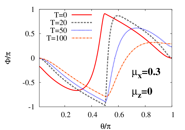
Figure 4: (Color online) The influence of varying temperature $T$ on the geometric phase $\Phi({\cal T})$ vs. initial state preparation $\theta$ is depicted for a dissipative qubit with $\mu_{x}=0.3$ and zero dephasing, i.e. $\mu_{z}=0$. The remaining parameters are the same as in Fig. 1. Temperature is measured in units of $\varepsilon/k_{B}$.

Thus far we considered zero temperature, $T=0$. The effect of increasing temperature is depicted in Fig. 4. Firstly, we observe that if temperature increases the phase does not vanish for $\theta\to\pi$ while it tends to zero for $\theta\to 0$. Secondly, the main properties remain similar: In all presented cases a minimum and a maximum exist. However, the maximum diminishes with increasing temperature.

5 Concluding remarks

No realistic physical quantum system is in perfect isolation from its environment. At best one can achieve a weak coupling between the system and the environment. In this weak coupling regime it is possible to extract the reduced dynamics of the open quantum system in a mathematically satisfactory and controlled way by using a Markovian reduced dynamics following the Davies scheme. In this work we have analyzed the geometric phase of a qubit in the presence of a weak coupling to a bosonic environment. We have investigated the relation between the geometric phase $\Phi$ and the mechanism for decoherence of the qubit for either the case of pure dephasing with $\mu_{x}=0$ or in presence of dissipative energy relaxation, i.e. $\mu_{x}\neq 0$. The latter situation allows for a significant variation of the emerging geometric phase upon varying the coupling strength $\mu_{x}$. A variation of the pure dephasing coupling, i.e. $\mu_{z}\neq 0$ with $\mu_{x}=0$, between qubit and environment barely affects the geometric phase. This feature is distinct from other set-ups, such as the emergence of quantum entanglement in open systems, where this dephasing-coupling mechanism can play a dominant or a similar role as an energy relaxation-coupling.

Nowadays, the geometric phase plays a crucial role in a variety of physical problems and has observable consequences in a wide range of systems. Under various aspects, this concept occurs in geometry, astronomy, classical mechanics, and quantum theory. The impressive recent progress in nanotechnology and experimental techniques allows one to test the fundamentals of quantum dynamics and details of interactions modeled by Hamiltonians. The geometric phase is not a quantum mechanical observable, i.e. it is not represented by a Hermitian operator. However, it can be experimentally measured, cf. Ref. exper . It can be used to encode information on systems. E.g. it has been proposed as an order parameter for quantum phase transitions ochnik . The results obtained here suggest that one can also exploit the geometric phase as a quantifier characterizing a nature of the system-environment coupling. Indeed, three features of the geometric phase $\Phi=\Phi({\cal T})$ allow one to distinguish the character of qubit-environment coupling (i.e. pure dephasing vs. dissipation): (i) rotation symmetry around some points on the $\theta-\Phi$ plane or equivalently antisymmetric dependence of $\Phi$ upon $\theta$ about some points, (ii) non-monotonic behavior of $\Phi$ with respect to $\theta$ and (iii) the behavior of $\Phi$ for $\theta\to 0$ (i.e. for the qubit prepared in the excited state). We have verified that all these three features are manifest also at times $t=n{\cal T}(n=2,3,4)$ for the measurable quantifier $\Phi=\Phi({n\cal T})$. This feature of the geometric phase $\Phi$ thus presents an additional suitable tool in exploring characteristics of open system interactions at the quantum scale.

References

- (1) Nielsen M. A., Chuang I. L.: Quantum Computation and Quantum Information. Cambridge University Press, Cambridge, (2000)
- (2) Lidar D. A., Whalley K. B.: Irreversible quantum dynamics. Lect. Notes in Physics, 622, 83, Springer, Berlin, (2006); Alicki R.: ibid, 121
- (3) Kohler S., Hänggi P.: Improving the purity of one- and two-qubit gates. Fortschr. Physik 54, 804-819 (2006)
- (4) Zanardi P., Rasseti M.: Holonomic quantum computation. Phys. Lett. A 264, 94-99 (1999)
- (5) Nayak C. et al.: Non-Abelian anyons and topological quantum computation. Rev. Mod. Phys., 80, 1083–1159 (2008)
- (6) Jones J. A., Vedral V., Ekert A., Castagnoli G.: Geometric quantum computation using nuclear magnetic resonance. Nature (London) 403, 869-871 (2000)
- (7) Sarandy M. S., Lidar D. A.: Adiabatic quantum computation in open systems. Phys. Rev. Lett. 95, 250503-250507 (2005)
- (8) Berry M. V.: Quantal phase factors accompanying adiabatic changes. Proc. R. Soc. London ser. A 329, 45-57 (1984); Wilczek F. Zee A.: Appearance of gauge structure in simple dynamical systems. Phys. Rev. Lett. 52, 2111-2114 (1984)
- (9) Duan L.-M., Cirac J. I., Zoller P.: Geometric manipulation of trapped ions for quantum computation. Science 292, 1695-1697 (2001)
- (10) Recati A., Calarco T., Zanardi P., Cirac J. I., Zoller P.: Holonomic quantum computation with neutral atoms. Phys. Rev. A 66, 032309-032322 (2002)
- (11) Yin Sun, Tong M. D.: Geometric phase of a quantum dot system in nonunitary evolution. Phys. Rev. A 79, 044303-044307 (2009)
- (12) Falci G., Fazio R., Palma G. M., Siewert J., Vedral V.: Detection of geometric phases in superconducting nanocircuits. Nature 407, 355-358 (2000); Faoro L., Siewert J., Fazio R.: Non-abelian phases, charge pumping and holonomic computation with Josephson junctions. J. Phys Soc. Jpn. 72, 3-4 (2003)
- (13) Parodi D., Sassetti M., Solinas P., Zanardi P., Zanghì N.: Fidelity optimization for holonomic quantum gates in dissipative environments. Phys. Rev. A 73, 052304-052309 (2006); Parodi D., Sassetti M., Solinas P., Zanghì N.: Environmental noise reduction for holonomic quantum gates. Phys. Rev. A 76, 012337-012343 (2007)
- (14) Uhlmann A.: The “transition probability” in the state space of a *-algebra. Rep. Math. Phys. 9, 273-279 (1976)
- (15) Bassi A., Ippoliti E.: Geometric phase for open quantum systems and stochastic uravellings. Phys. Rev. A 73, 062104-06111 (2006); Burić N., Radonjić M.: Uniquely defined geometric phase of an open system. Phys. Rev. A 80, 014101-014105 (2009)
- (16) Sjöqvist E. et al.: Geometric phases for mixed states in interferometry. Phys. Rev. Lett. 85, 2845-2849 (2000); Bhandari R.: Singularities of the mixed state phase. Phys. Rev. Lett. 89, 268901 (2002); Sjöqvist E.: Quantal interferometry with dissipative internal motion. Phys. Rev. A 70, 052109-052115 (2004); Bhandari R.: Polarization of light and topological phases. Phys. Reports 281, 1-64 (1997); Du J. et al.: An experimental observation of geometric phases for mixed states using NMR interferometry. Phys. Rev. Lett. 91, 100403-100407 (2003)
- (17) Mukunda N., Simon R.: Quantum kinematic approach to the geometric phase I. General formalism. Ann. Phys. 228, 205-268 (1993)
- (18) Tong D. M., Sjöqvist E., Kwek L. C., Oh C. H.: Kinematic approach to the mixed state geometric phase in nonunitary evolution. Phys. Rev. Lett. 93, 080405-080409 (2004)
- (19) Carollo A., Fuentes-Guridi I., França Santos M., Vedral V.: Geometric phase in open systems. Phys. Rev. Lett. 90, 160402-160406 (2003); Ericsson M., Sjöqvist E., Brännlund J., Oi D. K., Pati A. K.: Generalization of the geometric phase to completely positive maps. Phys. Rev. A 67, 020101-020105 (2003); Marzlin K.-P., Ghose S., Sanders B. C.: Geometric phase distributions for open quantum systems. Phys. Rev. Lett. 93, 260402-260406 (2004); Whitney R. S., Makhlin Y., Shnirman A., Gefen Y.: Geometric nature of the environment-induced Berry phase and geometric dephasing. Phys. Rev. Lett. 94, 070407- 070411 (2005); Sarandy M. S.,Duzzioni E. I., Moussa M. H. Y.: Dynamical invariants and nonadiabatic geometric phases in open quantum systems. Phys. Rev. A 76, 052112-052121 (2007)
- (20) Huang X. L., Yi X. X.: Non-Markovian effects on the geometric phase. Europhys. Lett. 82, 50001-50007 (2008)
- (21) Banerjee S., Srikanth R.: Geometric phase of a qubit interacting with a squeezed-thermal bath. Eur. Phys. J. D 46, 335-344 (2008); Fujikawa K., Hu M.-G.: Geometric phase of a two-level system in a dissipative environment. Phys. Rev A 79, 052107-052114 (2009); Wang Z. S., Liu G. Q., Ji Y. H.: Noncyclic geometric quantum computation in a nuclear-magnetic-resonance system. Phys. Rev. A 79, 054301-054305 (2009); Singh K. et al.: Geometric phases for nondegenerate and degenerate mixed states. Phys. Rev. A 67, 032106-032115 (2003)
- (22) Hänggi P., Ingold G. L.: Fundamental aspects of quantum Brownian motion. Chaos 15 026105-026115 (2005)
- (23) Alicki R., Fannes M. and Pogorzelska M.: Quantum generalized subsystems. Phys. Rev. A 79, 052111-052120 (2009)
- (24) Łuczka J.: Spin in contact with thermostat: Exact reduced dynamics. Physica A 167 919-934 (1990); Alicki R.: Pure decoherence in quantum systems. Open Sys. & Information Dyn. 11, 53-61 (2004)
- (25) Romero K. M. F., Talkner P., Hänggi P.: Is the dynamics of open quantum systems always linear? Phys. Rev. A 69, 052109-052117 (2004)
- (26) Dajka J., Mierzejewski M., Łuczka J.: Fidelity of asymmetric dephasing channels. Phys. Rev. A 79, 012104-012111 (2009)
- (27) Doll R., Wubs M., Hänggi P., Kohler S.: Limitation of entanglement due to spatial qubit separation. Europhys. Lett. 76, 547-553 (2006); Doll R., Wubs M., Hänggi P. Kohler S.: Incomplete pure dephasing of N-qubit entangled W states. Phys. Rev. B 76, 045317-045331 (2007); Dajka J., Mierzejewski M., Łuczka J.: Entanglement persistence in contact with the environment: exact results. J. Phys. A: Math. Theor. 40, F879-F886 (2007); Dajka J., Łuczka J.: Origination and survival of qudit-qudit entanglement in open systems. Phys. Rev. A 77, 062303- 062310 (2008); Doll R. , Hänggi P., Kohler S., Wubs M.: Fast initial qubit decoherence and the influence of substrate dimensions on error correction rates. Eur. Phys. J. B 68, 523-527 (2009)
- (28) Yi X. X., Wang L. C., Wang W.: Geometric phase in dephasing systems. Phys. Rev. A 71, 044101-044105 (2005); Yi X. X., Tong D. M. , Wang L. C., Kwek L. C., Oh C. H.: Geometric phase in open systems: Beyond the Markov approximation and weak-coupling limit. Phys. Rev. A 73, 052103-052109 (2006); Dajka J., Mierzejewski M., Łuczka J.: Geometric phase of a qubit in dephasing environment. J. Phys. A: Math. Theor. 41, F012001-F012008 (2008); Dajka J., Łuczka J.: Bifurcations of the geometric phase of a qubit asymmetrically coupled to the environment. J. Phys. A: Math. Theor. 41, F442001-F442009 (2008)
- (29) Davies E. B.: Markovian master equations. Comm. Math. Phys. 39, 91-110 (1974)
- (30) Dümcke R., Spohn H.: The proper form of the generator in the weak coupling limit. Z. Physik B 34, 419-422 (1979); Łuczka J.: On Markovian kinetic equations: Zubarev’s nonequilibrium statistical operator approach. Physica A 149, 245-266 (1988)
- (31) Lendi K., van Wonderen A. J.: Davies theory for reservoir-induced entanglement in a bipartite system. J. Phys. A: Math. Theor. 40, 279-288 (2007)
- (32) Schuster D. I. et al.: Resolving photon number states in a superconducting circuit. Nature 445, 515-518 (2007)
- (33) Alicki R., Lendi K.: Quantum dynamical semigroups and applications. Springer, Berlin (1987)
- (34) Aharonov Y., Ananadan J.: Phase change during a cyclic quantum evolution. Phys. Rev. Lett. 58, 1593-1597 (1987)
- (35) Chruściński D., Jamiołkowski A.: Geometric phases in classical and quantum mechanics. Birkhauser, Boston (2004)
- (36) Leek P. J. et al.: Observation of Berry’s phase in a solid-state qubit. Science 318, 1889-1892 (2007); Möttönen M. et al.: Experimental determination of the Berry phase in a superconducting charge pump. Phys. Rev. Lett. 100, 177201-177205 (2008); Fillipp S. et al.: Experimental demonstration of the stability of Berry’s phase for a spin-1/2 particle. Phys. Rev. Lett. 102, 030404-030408 (2009)
- (37) Nesterov A. I., Ovchinnikov S. G.: Geometric phases and quantum phase transitions in open systems. Phys. Rev. E 78, 015202-015206 (2008)