Near-Infrared Imaging Polarimetry of the Serpens Cloud Core: Magnetic Field Structure, Outflows, and Inflows in A Cluster Forming Clump

Abstract

We made deep near-infrared ($JHK$s) imaging polarimetry toward the Serpens cloud core, which is a nearby, active cluster forming region. The polarization vector maps show that the near-infrared reflection light in this region mainly originates from SVS2 and SVS20, and enable us to detect 24 small infrared reflection nebulae associated with YSOs. Polarization measurements of near-infrared point sources indicate an hourglass-shaped magnetic field, of which symmetry axis is nearly perpendicular to the elongation of the C¹⁸O ($J=1-0$) or submillimeter continuum emission. The bright part of C¹⁸O ($J=1-0$), submillimeter continuum cores as well as many class 0/I objects are located just toward the constriction region of the hourglass-shaped magnetic field. Applying the Chandrasekhar & Fermi method and taking into account the recent study on the signal integration effect for the dispersion component of the magnetic field, the magnetic field strength was estimated to be $\sim$100 $\mu$G, suggesting that the ambient region of the Serpens cloud core is moderately magnetically supercritical. These suggest that the Serpens cloud core first contracted along the magnetic field to be an elongated cloud, which is perpendicular to the magnetic field, and that then the central part contracted cross the magnetic field due to the high density in the central region of the cloud core, where star formation is actively continuing.

Comparison of this magnetic field with the previous observations of molecular gas and large-scale outflows suggests a possibility that the cloud dynamics is controlled by the magnetic field, protostellar outflows and gravitational inflows. Furthermore, the outflow energy injection rate appears to be larger than the dissipation rate of the turbulent energy in this cloud, indicating that the outflows are the main source of turbulence and that the magnetic field plays an important role both in allowing the outflow energy to escape from the central region of the cloud core and enabling the gravitational inflows from the ambient region to the central region. These characteristics appear to be in good agreement with the outflow-driven turbulence model and imply the importance of the magnetic field to continuous star formation in the center region of the cluster forming region.

1 Introduction

Stars are formed by gravitation in molecular clouds having both turbulence and magnetic fields in the Galaxy, and most of stars are thought to be formed in clusters (e.g., Lada & Lada, 2003; Allen et al., 2007). A mass spectrum of prestellar condensations is reported to have the power similar to that of the stellar IMF both in dust continuum observations (Reid & Wilson, 2006, and references therein) and molecular-line observations (e.g., Ikeda et al., 2007), and theoretical studies of turbulent molecular clouds (Klessen et al., 1998, and subsequent works) suggest that these condensations were formed through turbulent shock. One of the most promising sources of ordinary turbulence is outflows from protostars, which are ubiquitous in star forming regions and are believed to be formed through the mediation of magnetic field. Magnetic fields are also considered to play an important role in dynamical evolution of molecular clouds and control of star formation, i.e., formation of molecular cloud cores and their collapse (e.g., McKee & Ostriker, 2007).

Recently, Li & Nakamura (2006) and Nakamura & Li (2007) presented realistic 3D MHD simulations of cluster formation, taking into account the effect of protostellar outflows as well as initial turbulence and a magnetic field. In their simulations, they indicated that the initial turbulence is quickly replaced by turbulence generated by protostellar outflows, keeping the quasi-equilibrium state with a slow rate of star formation, and that magnetic fields are dynamically important if their initial strengths are not far below the critical value for static cloud support because of the amplification by the outflow-driven turbulent motions. The magnetic field is expected to influence the directions of outflow ejection and propagation and the transmission of outflow energy and momentum to the ambient medium. However, the magnetic field structures have not always been observationally clear in/around cluster forming regions, particularly around nearby cluster forming regions because of the lack of deep, wide-field near-infrared (NIR) polarimetry data.

The Serpens cloud core is one of the nearby, active low-mass star forming regions at the northern part of the Serpens cloud and many observational works have been done (Eiroa et al., 2008, and references therein). Recent mid-IR studies (e.g., Kaas et al., 2004; Harvey et al., 2007; Winston et al., 2007) revealed that a lot of embedded young stellar objects (YSOs), including Class 0/I objects, are located toward an aggregate of (sub)millimeter dust continuum cores (e.g., Davis et al., 1999; Kaas et al., 2004; Enoch et al., 2007), which consists of two sub-clumps (NW and SE sub-clumps; Olmi & Testi, 2002) in the central region and is enveloped by ambient molecular gas (e.g. ¹³CO, and C¹⁸O; McMullin et al., 2000; Olmi & Testi, 2002).

Many outflow activities that are related to star formation have been taking place in the Serpens cloud core. CO high velocity flows are reported to be widely spread over the cloud core (e.g., White et al., 1995; Davis et al., 1999; Narayanan et al., 2002). Compact molecular outflows of higher density tracers and H₂ jet-like knots are associated with the submillimeter cores (e.g., Curiel et al., 1996; Herbst et al., 1997; Wolf-Chae et al., 1998; Hodapp, 1999; Williams & Myers, 2000). The direction of these compact outflows was reported to be PA$\sim 155\arcdeg$ on an average with deviation of a few $10\arcdeg$ (see Table 5 of Olmi & Testi, 2002), which is nearly parallel to the alignment direction, from NW to SE, of the two sub-clumps (e.g., Davis et al., 1999; Kaas et al., 2004; Enoch et al., 2007), or to the cloud elongation in ¹³CO, C¹⁸O, and other higher density tracers (e.g. McMullin et al., 2000; Olmi & Testi, 2002). In addition, Davis et al. (1999) and Ziener & Eislöffel (1999) found, through optical narrow-band imaging, that many HH objects emanate from the two sub-clumps to the ambient region, penetrating the dense part of the central region.

The Serpens Reflection Nebula (SRN) illuminated by SVS 2 (Strom et al., 1976) has been extensively studied by polarimetric measurements both in optical and near-infrared (NIR) wavelengths (King et al., 1983; Warren-Smith et al., 1987; Gomez de Castro et al., 1988; Sogawa et al., 1997; Huard et al., 1997). NIR polarimetric measurements (Sogawa et al., 1997; Huard et al., 1997) probed also some other obscured reflection nebulae around SVS 2 in detail. Gomez de Castro et al. (1988) suggested the magnetic field of a NW-SE direction based on the elongation of the reflection nebulae around several YSOs in the central region of Serpens cloud core. In contrast, the NIR polarization measurement of a background star candidate suggested rather different direction of magnetic field because its polarization angle was nearly perpendicular to the NW-SE direction (Sogawa et al., 1997). However, this measurement was only for one background candidate, which in fact has a possibility of being a YSO in the Serpens cloud core and its polarization originating from the YSO itself. Therefore, it is vitally important to measure more background stars to resolve this discrepancy and to know the magnetic field structure toward the Serpens cloud core.

We conducted deep, $JHK$s imaging polarimetry of the Serpens cloud core to reveal the magnetic field structure in this region. We also searched for more NIR reflection nebulae associated with YSOs. Here, we present the results of our imaging polarimetry in the Serpens cloud core by comparing the data from the previous observations and discuss the role of the magnetic field in this region.

2 Observations and Data Reductions

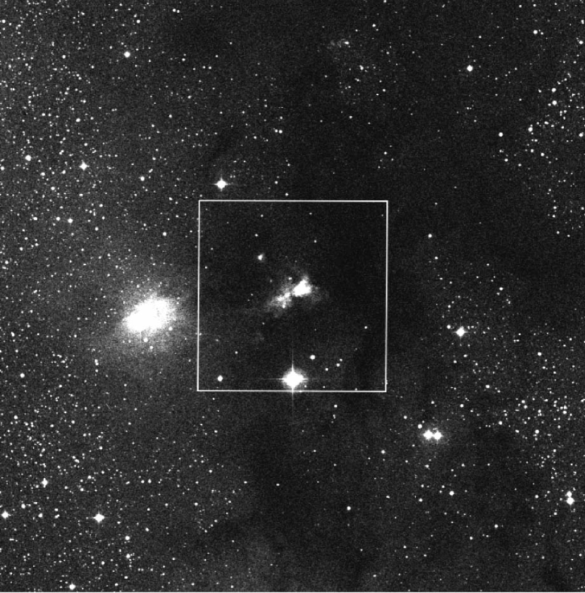
Figure 1: DSS II R image of the Serpens cloud core. The area of the polarimetric imaging is indicated by a rectangle with a size of $8.4\arcmin\times 8.5\arcmin$ and a center position of $(\alpha,{\mathit{\delta}})_{\rm J2000}$ =(18:29:57.6, +01:14:34).

Toward the Serpens cloud core (Figure 1), simultaneous $JHK$s polarimetric observations were carried out on 2006 June 23 UT with the imaging polarimeter SIRPOL (Kandori et al., 2006), which is an attachment of the near-infrared camera SIRIUS mounted on the IRSF 1.4-m telescope at the South Africa Astronomical Observatory. The SIRIUS camera is equipped with three 1024 $\times$ 1024 HgCdTe (HAWAII) arrays, $JHK$s filters, and dichroic mirrors, which enables simultaneous $JHK$s observations (Nagashima et al., 1999; Nagayama et al., 2003). The field of view at each band is $\sim$7$\farcm$7 x 7$\farcm$7 with a pixel scale of 0$\farcs$45 pixel^-1.

We obtained 10 dithered exposures, each 10 s long, at four wave-plate angles (0$\arcdeg$, 22.5$\arcdeg$, 45$\arcdeg$, and 67.5$\arcdeg$ in the instrumental coordinate system) as one set of observations and repeated this 9 times. Sky images were also obtained in between target observations. Thus, the total on-target exposure time was 900 s per wave-plate angle. The seeing was $\sim 1.2\arcsec$ at $K$s during the observations. Twilight flat-field images were obtained at the beginning and end of the observations.

Standard procedures, dark subtraction, flat-fielding with twilight-flats, bad-pixel substitution, sky subtraction, and averaging of dithered images, were applied with IRAF. We first calculated the Stokes parameters as follows; $Q=I_{0}-I_{45}$, $U=I_{22.5}-I_{67.5}$, $I=(I_{0}+I_{22.5}+I_{45}+I_{67.5})/2$, where $I_{0}$, $I_{22.5}$, $I_{45}$, and $I_{67.5}$ are intensities at four wave-plate angles. To obtain the Stokes parameters in the equatorial coordinate system, a rotation of 105$\arcdeg$ (Kandori et al., 2006) was applied to them. We calculated the degree of polarization $P$, and the polarization angle $\theta$ as follows; $P=\sqrt{Q^{2}+U^{2}}/I$, $\theta=(1/2)\tan^{-1}(U/Q)$. The polarization intensity ($PI$) is obtained by multiplying the total intensity ($I$) by the degree of polarization ($P$). The absolute accuracy of the position angle of polarization was estimated to be better than 3$\arcdeg$ at the first light observation of SIRPOL (Kandori et al., 2006). The polarization efficiencies are 95.5%, 96.3%, and 98.5% at $J$, $H$, and $K$s, respectively, and the instrumental polarization is less than 0.3% all over the field of view at each band (Kandori et al., 2006). Due to these high polarization efficiencies and low instrument polarization, no particular corrections were made here.

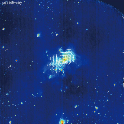
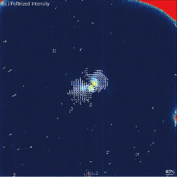
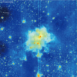
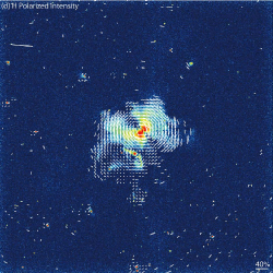
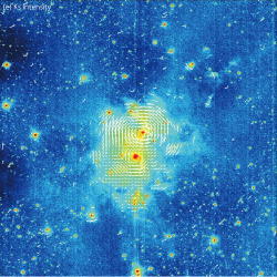
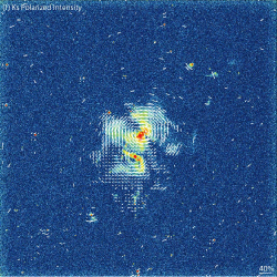
Figure 2: $JHK$s polarization vector maps of the Serpens cloud core, superposed on the total and polarized intensity images in the logarithmic scale. The vectors were made by 12$\times$12 pixel binning. The field of view is $\sim 7\farcm 7\times 7\farcm 7$. North is at the top and east is to the left. The center position of each image is $(\alpha,{\mathit{\delta}})_{\rm J2000}$ =(18:29:57.39, +01:14:36.2). The dead pixel regions of the $J$-band images are at the upper right and near the middle of the right edge.

Aperture polarimetry was performed for $H$ and $K$s band point sources detected by DAOFIND in the field of view. No polarimetry for J band sources was done due to their much smaller number, compared with those of $H$ and $K$s band sources (see Figure 2 a, c, and e). APHOT of the DAOPHOT package was used to evaluate the point source magnitudes for four wave-plate angles at $H$ and $K$s. An aperture radius of 3 pixels was adopted for each band. The errors of the degree of polarization (${\mathit{\Delta}}P$) and the position angle were calculated from the photometric errors, and the degrees of polarization were debiased as $P_{\rm debias}=\sqrt{P^{2}-{\mathit{\Delta}}P^{2}}$ (Wardle & Kronberg, 1974). Hereafter, we use $P$ as substitute for this debiased value for the aperture photometry data. Only the sources with photometric errors of $<$0.1 mag and $P/{\mathit{\Delta}}P>2$ were used for analysis. The 2MASS catalog (Skrutskie et al., 2006) was used for absolute photometric calibration. The limiting magnitudes at 0.1 mag error level were estimated to be 18.6 at $H$ and 17.5 at $K$s.

3 Results

3.1 Polarizations of extended emission

The $JHK$s polarization vector maps of the Serpens cloud core are shown, superposed on the total and polarization intensity images in Figure 2. These polarization maps clearly indicate that the central part of the reflection nebula is illuminated mainly by two sources; the north part (SRN) by SVS 2 and the south part by SVS 20, at $H$ and $K$s with two centrosymmetric patterns (see also Sogawa et al., 1997; Huard et al., 1997), while at $J$ only SRN is dominant (see also Sogawa et al., 1997) as is seen in the optical (Warren-Smith et al., 1987; Gomez de Castro et al., 1988). This invisibleness at shorter wavelengths suggests that the southern part of SRN around SVS 20 is more obscured than the northern part around SVS 2, consistent with the $A_{V}$ map deduced from $H-K$ color (Huard et al., 1997). The centrosymmetric patterns are more clearly shown in Figure 3, which is a $K$s polarization vector map shown with a resolution higher than Figure 2e.

The $PI$ images and vector patterns of SVS 2 clearly show that SVS 2 is associated with a bipolar structure with a dark lane. In the $JHK$s intensity images of Figures 2 a, c, and e, at shorter wavelengths, the NW lobe of the bipolar nebula is brighter than the SE lobe, while at longer wavelengths the SE lobe is brighter. This suggests that the NW lobe is near side and that the SE lobe is far side. The nebula structure and dark lane of SRN have been already reported in the two polarimetric studies (Sogawa et al., 1997; Huard et al., 1997). In addition, Pontoppidan & Dullemond (2005) modeled SRN as a disk shadow system with their imaging data, and suggested that SVS 2 is associated with a small disk, which is not unresolved, and a spherically symmetric envelope.

The nebula illuminated by SVS 20 is clearly recognized at $H$ and $K$s with a centrosymmetric pattern around SVS 20. This object has a peculiar morphology with a ring and two arms protruded from that ring. Because we plan to report its details in a separate paper, including other YSOs with reflection nebulae, we will not mention the details here.

3.2 Polarizations of nebulosities associated with YSOs

3.2.1 The central region

Figure 3 presents an higher resolution $K$s polarization vector map with 3$\times$3 pixel binning toward the central region of the overall image, superposed on the $K$s intensity map. With this map and/or the highest resolution vector maps without binning, we identified stellar sources having reflection nebulae locally illuminated by themselves with centrosymmetric or centrosymmetric-like patterns. It is not easy to identify such sources only from Figure 3 due to the strong contamination from SVS 2 and SVS 20. It is also not easy toward the SVS 4 cluster, which is a compact cluster located to the south of SVS 20, due to the source congestion. We therefore used the highest resolution vector maps without binning for the sources having the strong contamination (see Appendix). The identified sources with reflection nebulae illuminated by themselves are marked in Figure 3, including SVS 2 and SVS 20, and are listed in Table 1.

Most of the identified sources are relatively bright in the central region. This is probably due to the strong light from SVS 2 and SVS 20 and only brighter sources with reflection nebulae may be detected. Except EC117 (SSTc2dJ 18300065+0113402), all the identified sources are classified as sources that have outer disks with an excess at least 8 and/or 24 $\micron$, i.e., class 0/I, flat spectrum, class II and transition disk sources (Winston et al., 2007). Although EC117 is classified as a class III source without an outer disk due to no detection of $24\micron$ continuum (Table 4 of Winston et al., 2007), it was reported that EC117 has a flux of 3.20$\pm$1.43 mJy at $24\micron$ (Table 3 of Harvey et al., 2007). This could suggest the outer disk of EC117, but the signal to noise ratio of $\sim$2 is not high enough for the robust detection at $24\micron$. Almost all members of the SVS 4 cluster seem to be associated with reflection nebulae.

3.2.2 The NW region

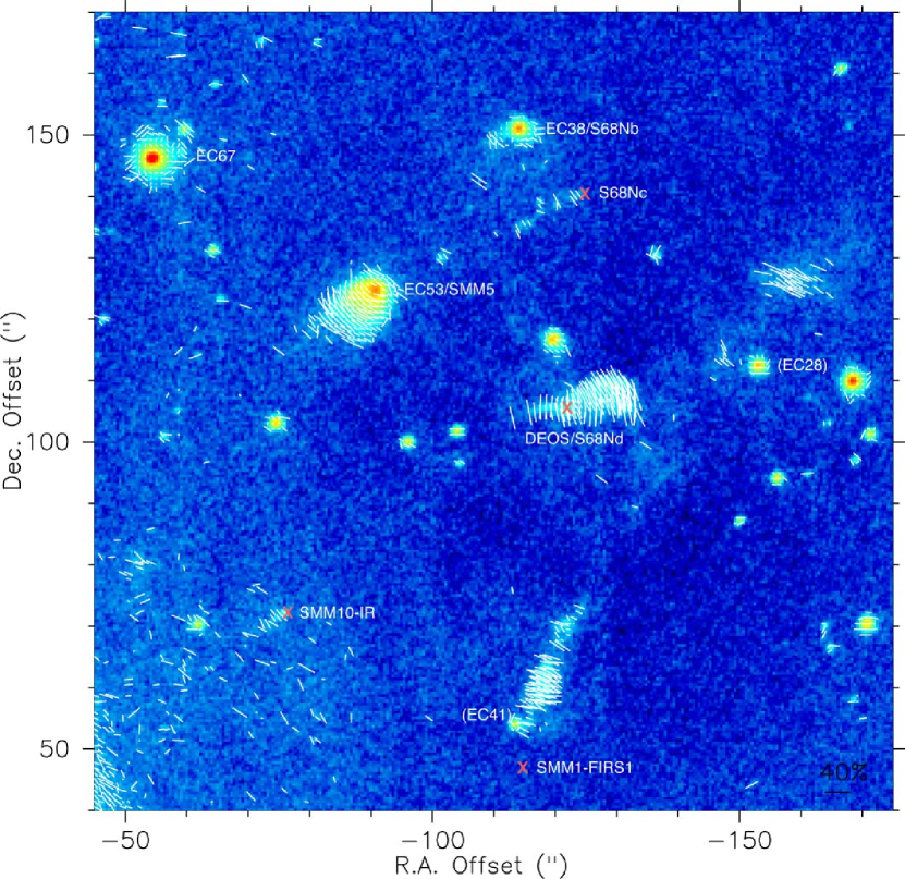
Figure 4: $K$s polarization vector map of the NW sub-core region of the Serpens cloud core, superposed on the total intensity images in the logarithmic scale. The vectors were shown every 2 pixels. The area of the image is $130\arcsec\times 130\arcsec.$ The reference position of offset is $(\alpha,{\mathit{\delta}})_{\rm J2000}$ =(18:29:57.39, +01:14:36.2). North is at the top and east is to the left. 40% vector is shown near the bottom right corner. The young stellar objects with reflection nebulae are marked, but EC28 and EC41 are not identified as young stellar objects with reflection nebulae.

Figure 4 presents a high resolution $K$s polarization vector map without binning toward the NW region of SRN. Here we identified stellar sources associated with self-luminous nebulae as well as those with reflection nebulae by using this map and listed them in Table 2. Three sources, DEOS, EC53, and EC67, are associated with reflection nebulae having centrosymmetric or partially centrosymmetric vector patterns. The other sources are associated with elongated nebulae or jet-like knots emanating from the sources in a straight line and their polarization vectors are almost perpendicular to their elongation directions. The elongated structures or knots are likely to be created/excited by outflows from these sources.

The jet-like knots are clearly seen near the north-west of EC41, which was considered to be an embedded star but not a driving source of this jet (Eiroa & Casali, 1989; Hodapp, 1999). These jet-like knots are reported to be mostly H₂ emission with weak continuum (Hodapp, 1999), and their polarization of these knots is nearly perpendicular to the jet elongation, though the polarization directions are more scattered in the northern knots than in the southern knots of this jet-like structure. At $H$-band, the polarization vectors of weak continuum emission of the southern knots are also nearly perpendicular to the jet elongation, which is parallel to the radial direction from SMM1-FIRS1, not from EC41. Thus, SMM1-FIRS1 is the illuminating source of these jet-like knots, and the jet-like knots could correspond to the cavity walls that were created by the outflow from SMM1-FIRS1.

The jet-like structure from SMM1-FIRS1 seems to continue farther away to a bow-shock-like nebulosity located at $\sim$80-90$\arcsec$ north-west of SMM1-FIRS1 (or at $\sim 20\arcsec$ north-west of EC28). The polarization vectors at this bow nebulosity indicate either SMM1-FIRS1 or EC28 is illuminating or exciting it. No information is available on whether the bow nebulosity is really shock-excited H₂ emission or not, due to its position outside Figure 3 of Hodapp (1999), although week $H$-band continuum emission is detectable with polarization angles similar to those of $K$s-band. The alignment with the jet structure, the bow nebulosity and HH 460, which is located at $\sim 4\arcmin$ north-west to SMM1-FIRS1 (Davis et al., 1999), gives a hint that the bow nebulosity is related to the outflow from SMM1-FIRS1. The associations of the blueshifted CO lobe with HH 460 (Davis et al., 1999) and of the bow nebulosity with the CS emission (CS1; Testi et al., 2000), which is considered to be related to the outflow, support the shock excitation of the bow nebulosity. However, it is impossible to completely exclude the possibility that EC28, which is the closest NIR source to the bow nebulosity, or SMM1-FIRS1 itself contributes to the illumination of the bow nebulosity, due to the scattering of the polarization vector directions. In the midway from SMM1-FIRS1 to this bow nebulosity, there exist some faint knots that are almost H₂ emission (see Figure 3 of Hodapp, 1999), but no polarization is detectable for these knots.

The chain of nebulosity knots, located just south-east to the 3 mm continuum core S68Nc (Testi & Sargent, 1998; Williams & Myers, 2000), was reported to be H₂ emission jets that originate from the 3mm subknot a3/S68Nc (Hodapp, 1999). Although only several polarization vectors are shown toward these knots, they could imply that their polarization direction is nearly perpendicular to the jet elongation.

A nebulosity protruding from EC38/S68Nb is seen, and its polarization vectors appear to be nearly perpendicular to the protruding direction. A faint, small, elongated nebulosity is recognized just south-east to SMM10-IR. Although some nebulosities illuminated from SVS 2 are also seen near SMM10-IR, this nebulosity is most likely a nebulosity related to SMM10-IR based on its morphology. No information is available on whether these two nebulosities are shock-excited H₂ emission or not, because they are out of Figure 3 of Hodapp (1999). We note that no $H$-band emission is detectable toward SMM10-IR, while very week $H$-band continuum is seen toward the nebulosity protruding from EC38/S68Nb.

3.3 Polarizations of point sources

We have measured $H$ and $K$s polarization for point sources, in order to examine the magnetic field structures. Only the sources with photometric errors of $<$0.1 mag and $P/{\mathit{\Delta}}P>3$ were used for analysis.

The top panel of Figure 5 presents the polarization degrees at $H$ versus $H-K$s color diagram for sources having polarization errors of $<0.3\%$. YSOs identified by Winston et al. (2007) are not included in this diagram. In this diagram, the maximum of polarization degree at an $H-K$ color is roughly proportional to the $H-K$ color, i.e., the extinction, having consistency that the origin of the polarization is dichroic absorption. Therefore, we consider the polarization of these point sources as the polarization of the dichroic origin, and that their polarization vectors represent the directions of the local magnetic field averaged over their line of sight of the sources. In the nearby star forming regions such as the Taurus and Ophiuchus clouds, the highest value of the maximum polarization efficiency was reported to be $P(H)/E(H-K)=4.6$ or $P(H)/A(H)=1.6$ (Kusakabe et al., 2008), which were derived from the data of Whittet et al. (2008). In Figure 5, a dashed line represents $P(H)/(H-K\rm{s})=4.6$ where the offset of the intrinsic $H-K\rm{s}$ color is ignored. Our sources have the maximum polarization efficiency of $P(H)/(H-K\rm{s})=6.2$ (thick line) similar to that of the nearby star forming regions, and this is also consistent with the dichroic origin.

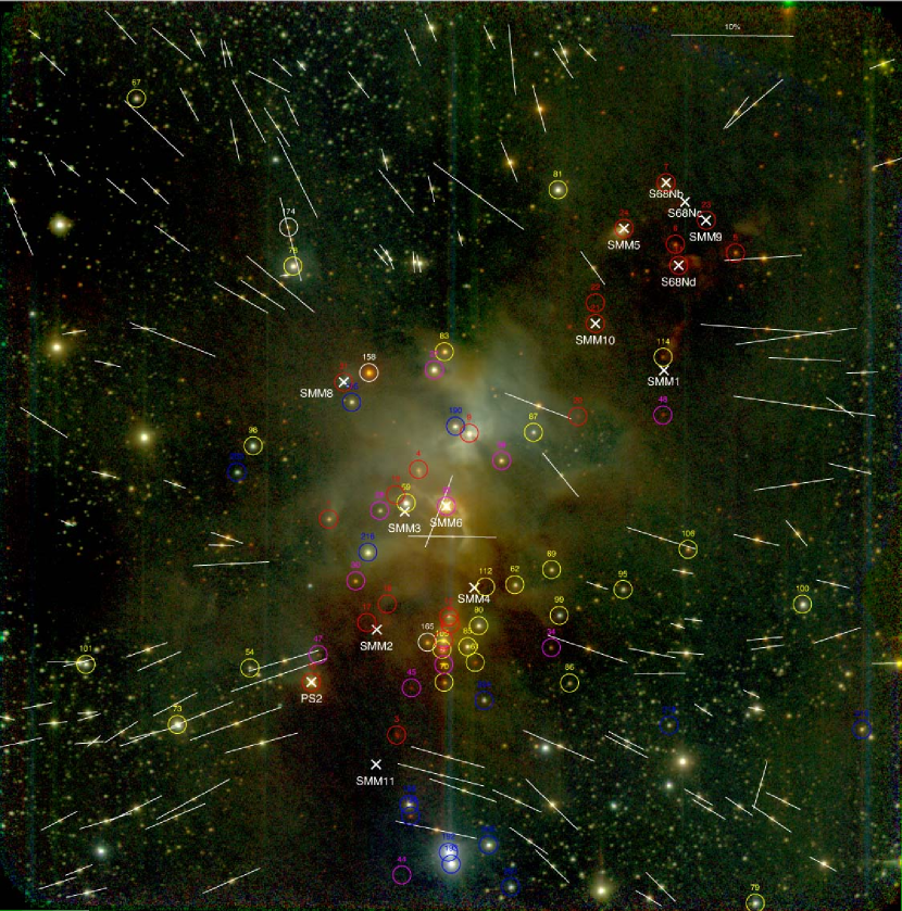
Figure 6: $H$-band polarization vectors (white bars) for point sources having $P/{\mathit{\Delta}}P>3$ and $P<6.2(H-Ks)$, superposed on a $JHK$s composite color image in the logarithmic scale. 10% vector is shown near the upper right corner. The area of the image ($\sim 8\farcm 4\times 8\farcm 5$) made by averaging the dithered frames is slightly larger than that of the camera array ($\sim 7\farcm 7\times 7\farcm 7$). North is at the top and east is to the left. YSOs identified by the Spitzer space telescope are marked by circles (Class 0/I; red, Flat-spectrum; magenta, Class II; yellow, Transition disk; blue, Class III; white) with ID numbers (Tables 3 and 4 of Winston et al., 2007). Submillimeter continuum peaks are show by crosses with names and their coordinates come from the Spitzer photometry of Winston et al. (2007), except SMM2 and SMM11 (Davis et al., 1999).

The bottom panel of Figure 5 shows the $H$-band polarization angles of the point sources with $P<6.2(H-K\rm{s})$, of which the polarization vectors are shown in Figure 6. YSOs are not included in the bottom panel, but included in Figure 6.

The polarization angles are mostly in a range of $\sim$0–140$\arcdeg$ and their median and average angles are 63.5$\arcdeg$ and 64.6$\pm$35.6$\arcdeg$, respectively. While the polarization angles are largely scattered, there is a tendency that the degree of scatter becomes smaller in the redder $H-K\rm{s}$ color region. This tendency suggests that the polarization angles are more confined in the inner region (redder color region) than in the outer region.

The magnetic field is neither simply straight nor random over the whole field (Figure 6). The vectors appear to be systematically ordered and gradually curved, suggesting a clear hourglass shape that is left-handedly tilted by $\sim 60$–$80\arcdeg$ and the direction of the global magnetic field that is nearly perpendicular to the elongation of the Serpens cloud core from NW to SE, $\sim 150\arcdeg$ (e.g., the C¹⁸O maps of McMullin et al., 2000; Olmi & Testi, 2002).

Signs of hourglass shapes in the magnetic field have been already reported in high-mass star forming cores such as NGC 2024 (Lai et al., 2002), OMC-1 (Schleuning, 1998; Houde et al., 2004; Kusakabe et al., 2008), and DR21 Main (Kirby, 2009). In low mass cores such as NGC 1333 IRAS 4A (Girart et al., 2006) and Barnard 68 (Kandori et al., 2009) hourglass shapes have been more clearly shown. These examples, except OMC-1, of the hourglass-shaped magnetic field have been found only in isolated cores or cores with simple structures in the star forming regions. However the Serpens cloud core is a molecular cloud complex consisting of many molecular cloud cores or sub-millimeter cores (e.g., Davis et al., 1999), which form a cluster of low-mass YSOs, and the hourglass-shaped magnetic field spreads widely over the Serpens cloud core. Thus, this is a clear example that the hourglass-shaped magnetic field is associated with a low-mass star forming complex, while OMC-1 is an example of a hight-mass star forming complex.

4 Analysis and Discussion

4.1 Shape of the magnetic field

We have modeled the shape of the magnetic field with the polarization vectors measured at $H$ for point sources, following Girart et al. (2006) and Kandori et al. (2009). The magnetic field was fitted with a parabolic function of $x=g+gCy^{2}$, with a counterclockwise tilted $y$-axis (the parabolic magnetic field axis of symmetry) by $\theta_{\rm PA}$ and a symmetric center $(x,y)_{\rm center}$, where the $y$ is the distance from the horizontal axis ($x=0$) and the $x$ is the distance from the parabolic magnetic field axis of symmetry. The value of $\tan^{-1}(dy/dx)+90\arcdeg$ corresponds to the position angle of the polarization ($\theta$). Only the point sources, except YSOs, having $P/{\mathit{\Delta}}P>3$ and $P<6.2(H-Ks)$, were used for the fitting. The error of the polarization angle (${\mathit{\Delta}}\theta$) was used to compute a weight for the datum, $1/({\mathit{\Delta}}\theta)^{2}$.

In Figure 7, the best-fit magnetic field is shown as well as the measured polarization vectors for 149 sources. The position angle of the parabolic magnetic field axis of symmetry is $\sim 70\arcdeg$, and the coefficient $C$ of $y^{2}$ is $\sim 7.1\times 10^{-6}$ pixel^-2. The root mean square (r.m.s.) of the residuals is $\sim 22\arcdeg$.

We executed one-parameter fitting of the magnetic field in local areas, in order to more accurately calculate the r.m.s. of the residuals, with the same $\theta_{\rm PA}$ and $(x,y)_{\rm center}$ obtained in the global fitting above. We selected three corners and one more area of the image where the source density is relatively high and/or the magnetic field seems to be rather ordered (areas outlined by dashed boxes in Figure 7). Toward the SE corner of the image ( $x<400$ and $y<400$ in Figure 7; 30 sources), the coefficient $C$ of $y^{2}$ was determined to be $(7.99\pm 0.76)\times 10^{-6}$ pixel^-2, similar to that of the global fitting, and the r.m.s. of the residual was calculated to be $12.9\pm 0.9\arcdeg$, and toward the SW corner ($x>500$ and $y<230$; 20 sources), $C=(7.52\pm 1.00)\times 10^{-6}$ pixel^-2 and r.m.s. = $27.0\pm 2.0\arcdeg$ were obtained. Removing the dispersion due to the measurement uncertainties of the polarization angles $4.2\pm 3.0\arcdeg$ and $3.2\pm 2.2\arcdeg$, we obtained the dispersions from the best-fit model, $12.2\pm 1.4\arcdeg$and $26.8\pm 2.0\arcdeg$ for the SE and SW corners, respectively. Toward the NE corner ($x<300$ and $y>800$; 18 sources), $C=(3.36\pm 0.92)\times 10^{-6}$ pixel^-2 and r.m.s. = $14.8\pm 1.6\arcdeg$ were evaluated, and the intrinsic dispersion from our model of $13.7\pm 2.0\arcdeg$ was obtained with the measurement uncertainty of $5.6\pm 2.4\arcdeg$. This smaller $C$ indicates that the curvature of the magnetic field here is rather looser than that expected from the global fitting, i.e., slightly bended to the direction parallel to the symmetry axis of the magnetic field. Toward the area next to the NE corner ($400<x<700$ and $y>800$; 17 sources), $C=(6.85\pm 0.55)\times 10^{-6}$ pixel^-2 and r.m.s. = $13.3\pm 1.4\arcdeg$ were evaluated, and the intrinsic dispersion of $12.6\pm 1.8\arcdeg$ was obtained with the measurement uncertainty of $4.2\pm 2.9\arcdeg$.

4.2 Comparison of the magnetic field with the submillimeter and millimeter data

4.2.1 850 $\micron$ continuum

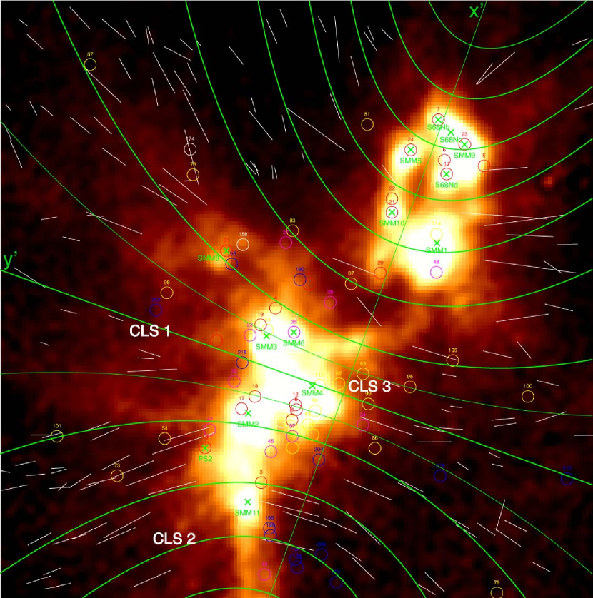
Figure 8: $H$-band polarization vectors (white lines) for point sources having $P/{\mathit{\Delta}}P>3$ and $P<6.2(H-K$s), and their best-fit magnetic field (green thick curved/ straight lines and thin curved lines), superposed on SCUBA 850 $\micron$ continuum image (kindly provided by C.J. Davis, see Figure 1 of Davis et al., 1999). Note that these lines do not present lines of magnetic force, just the direction of the magnetic field. The horizontal axis (green thin straight line), which is perpendicular to the parabolic magnetic field axis (green thick straight line), is also shown. The area of the image is $\sim 8\farcm 4\times 8\farcm 5$, same as that of Fig. 6. North is at the top and east is to the left. The YSOs identified by the Spitzer space telescope and submillimeter continuum peaks are indicated the same as in Figure 6.

We compare our $H$-band measured polarization vectors and the modeled magnetic field with the 850 $\micron$ dust continuum map of Davis et al. (1999) in Figure 8. Note that the green lines of this figure do not present lines of magnetic force, just the direction of the magnetic field.

The high intensity ridge of the 850 $\micron$ continuum is elongated along the NW-SE direction, having two sub-clumps (NW and SE sub-clumps), both of which consist of several dense cores (e.g., SMM 1–11, S68Nb–d, and PS2 in Figure 8). This distribution of the 850 $\micron$ continuum is very similar to that of the bright parts of the ¹³CO($J=1-0$) and C¹⁸O($J=1-0$) emission (McMullin et al., 2000; Olmi & Testi, 2002), although the global distribution of the ¹³CO($J=1-0$) emission is not always elongated, but rather roundly extended (Olmi & Testi, 2002). It is evident that the symmetric axis ($y^{\prime}$-axis) of the best-fit magnetic field with a parabolic function is nearly perpendicular to the elongation direction of these continuum and molecular line emissions. The horizontal axis ($x^{\prime}$-axis) of the parabolic magnetic field is situated nearly along the 850 $\micron$ continuum ridge, although there are some deviations of the continuum emission from the horizontal axis. The symmetric axis of the parabolic magnetic field runs through the northern part of the SE sub-clump, not through the middle point of the two sub-clumps, which looks like the center of gravity of the Serpens cloud core when we glance at the 850 $\micron$ continuum map.

Davis et al. (1999) suggested the presence of three extended cavity-like structures to the east of SMM 3 (hereafter CLS 1), south-west of SMM 2 (hereafter CLS 2), and north-west of SMM 4 (hereafter CLS 3), which consist of three pairs of filaments that protrude the 850 $\micron$ continuum ridge. They mentioned that these cavity structures (CLS 1–3) are probably shaped by outflows rather than by global cloud collapse along, say, magnetic field lines.

As is in Figure 8, the filaments to the north-east of SMM 3 and east of SMM 2 form CLS 1, those to the south-east of SMM2/PS2 and south of SMM11 form CLS 2, and those to west of SMM3 and east of SMM4 form CLS 3. It appears that the two filaments of CLS 1 jut almost along the magnetic field from the SE sub-clump and that the symmetry axis ($y^{\prime}$-axis) of the magnetic field go through the inside of CLS 1 as well as CLS 3.

4.2.2 CO emission

Here we compare our best-fit magnetic field with the ¹²CO $J=2-1$, ¹²CO $J=1-0$, ¹³CO $J=1-0$, and C¹⁸O $J=1-0$ observations (White et al., 1995; Davis et al., 1999; McMullin et al., 2000; Narayanan et al., 2002; Olmi & Testi, 2002).

¹²CO $J=2-1$

As was mentioned above, the bright parts of the ¹³CO $J=1-0$ and C¹⁸O $J=1-0$ emission maps are elongated and confined in the ridge, while the global distributions of ¹²CO $J=2-1$ and ¹³CO $J=1-0$, i.e., the low density molecular gas, are extended (e.g., White et al., 1995; Davis et al., 1999; Olmi & Testi, 2002).

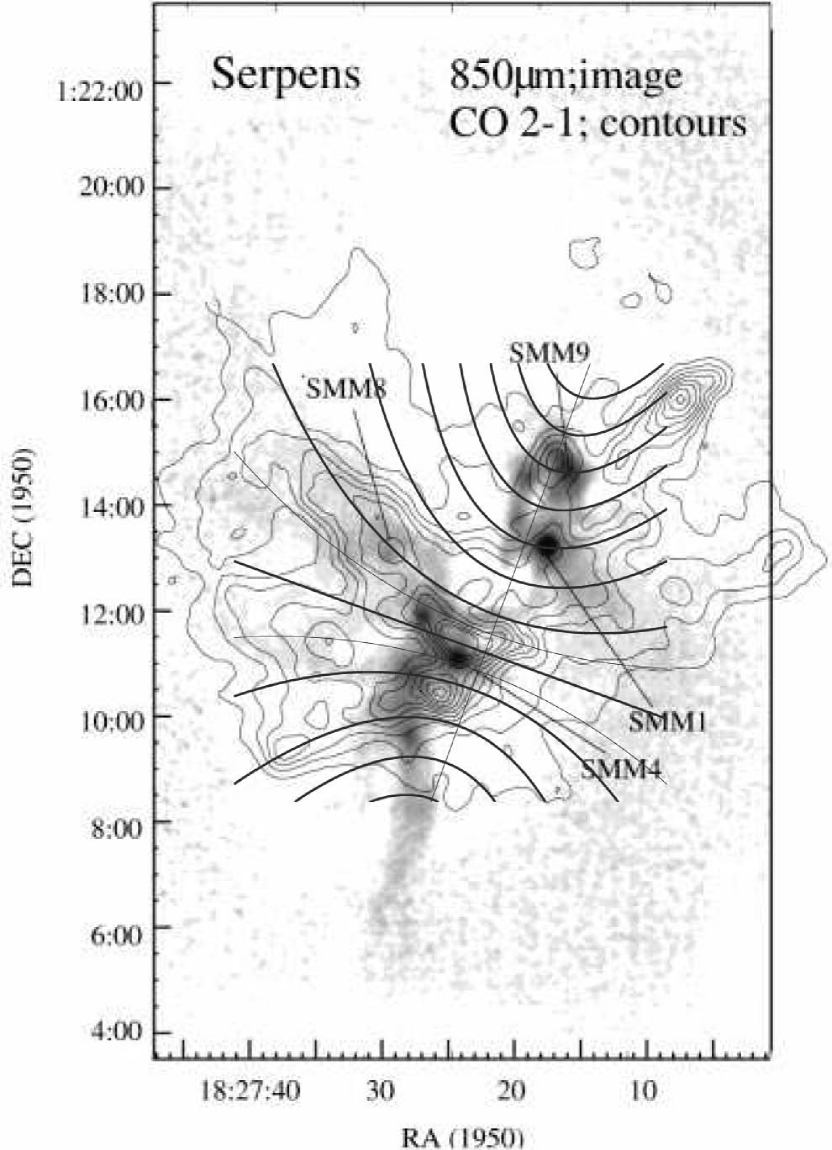
Figure 9: The best-fit magnetic field (the same as Figure 8), superposed on the CO $J=2-1$ contour plot of $V_{\rm LSR}$=2–16 km s^-1 and 850 $\micron$ continuum image (Figure 2 of Davis et al., 1999).

Figure 9 presents our best-fit magnetic field superposed on the CO $J=2-1$ contour map and 850 $\micron$ image of Davis et al. (1999), where the CO $J=2-1$ map is considered to show the ambient molecular gas of the Serpens cloud core, but not the dense cores. Davis et al. (1999) mentioned that toward the two filaments of CLS 1 and one CLS 2 filament to the south-east of SMM2/PS2 the CO $J=2-1$ emission and 850 $\micron$ continuum distributions coincide well. As mentioned above, the two filaments seem to run almost along the magnetic field, indicating that the CO $J=2-1$ filaments are also related with the magnetic field. For the CLS 2 filament to the south-east of SMM2/PS2, the same situation as the CLS 1 filaments may be also seen. Two other CO $J=2-1$ filaments/extensions to the north-west of SMM 9 and west of SMM 1 are also noticeable in Figure 9. Although considerable parts of these two filaments are out of our polarimetry image, the extrapolation of our best-fit magnetic field cloud predict that these two filaments run along the magnetic lines.

C¹⁸O $J=1-0$ and ¹³CO $J=1-0$

McMullin et al. (2000) showed that a velocity gradient running from a LSR velocity centroid of 9 km s^-1 at the north-west end of the C¹⁸O $J=1-0$ emission to 7.5 km s^-1 at the south-east end (Figure 2 of McMullin et al., 2000), i.e., along the elongation direction of C¹⁸O. On the other hand, Olmi & Testi (2002) suggested that the Serpens cloud exhibits a velocity gradient roughly from east to west, based on their model fitting of velocity gradients in C¹⁸O $J=1-0$, ¹³CO $J=1-0$, C³⁴S $J=1-0$, adopting their map center, which is the middle point of the two sub-clumps, as the reference position for analysis. However, according to their channel and centroid velocity maps (Figures 7 and 8 of Olmi & Testi, 2002), the bright parts of C¹⁸O $J=1-0$ and ¹³CO $J=1-0$ are similar to that of McMullin et al. (2000), and a steep velocity gradient from NW to SE almost along the normal line of the symmetry axis ($y^{\prime}$-axis) of the magnetic field can be seen at just south of their reference position in ¹³CO, although at the reference position a velocity gradient from West to East is seen. It is surprising that the normal line of the steep velocity gradient almost coincides with the symmetry axis ($y^{\prime}$-axis) of the magnetic field.

In summary, the direction of velocity gradient is nearly along the elongation of the Serpens cloud core and is nearly perpendicular to the symmetry axis of the magnetic field with a coincidence of the normal line of the steep velocity gradient and the axis of the magnetic field. It could be possible that this normal line of the velocity gradient is an axis of the global rotation of the Serpens cloud core if the real center of gravity of the Serpens cloud core is located on the symmetry axis of the magnetic field.

It is interesting to examine the presence of C¹⁸O $J=1-0$ and ¹³CO $J=1-0$ features that coincide with the filaments of the CO $J=2-1$ emission and 850 $\micron$ emission. In the C¹⁸O $1-0$ integrated emission maps of White et al. (1995), McMullin et al. (2000) and Olmi & Testi (2002), a feature to the north-east of SMM 3 could coincide with one of the CSL 1 filament, but one to the east of SMM 2 is not clear. In the channel map of ¹³CO $J=1-0$ (Figure 7 of Olmi & Testi, 2002), a filament feature to the east of SMM 2 is clearly visible in the blue-shifted emission at the panel of $V_{\rm LSR}$=5–7.3 km s^-1. This filament looks likely to coincide with the CSL 1 filament to the east of SMM 2, but we can clearly recognize that it is located just outside this CSL 1 filament, i.e., between this CSL 1 filament and the CSL 2 filament to the south-east of SMM 2/PS2. At the same panel, a feature to the north and north-east of SMM 3 or near SMM 8 is also visible. This feature appears to be just outside the CLS 1 filament to the north-east of SMM 3. At the panel of $V_{\rm LSR}$=8.4–12.4 km s^-1, a red-shifted feature that protrudes from the SE sub-clump is visible, but it is located toward the inside region of CLS 1. The presence of this red-shifted feature and the blue-shifted features are probably consistent with red-shifted velocity region that jut from the SE sub-clump and with blue-shifted regions toward both sides of this red-shifted region, respectively, in the ¹³CO $J=1-0$ centroid velocity map of Olmi & Testi (2002).

CO outflows

Davis et al. (1999) presented the integrated intensity contours of CO $J=2-1$ blue- and red-shifted outflows (Figures 4 and 8 of Davis et al., 1999). These figures imply that the 850 $\micron$ filaments that coincide the CO $J=2-1$ filaments are shaped by outflows. On the basis of a fact that these filaments run along the magnetic field, the outflows that protruded from the ridge to its ambient are most likely to be guided by the magnetic field or to drag the magnetic field. The outflows may be guided by the magnetic field since the magnetic field seems to be strong enough to be ordered at least over our polarimetric imaging area.

The CLS 1 filaments are associated with red-shifted outflows, but no red-shifted CO $J=2-1$ emission is visible at the root of CLS 1. However, CO $J=1-0$ obervations (Narayanan et al., 2002) showed U-shaped, red-shifted high velocity flow at the root of CLS 1. This CO $J=1-0$ feature and our best-fit magnetic field support the idea of Davis et al. (1999) that the CLS 1 filaments of the CO $J=2-1$ and 850 $\micron$ emission illustrate the action of a wide-angled wind powered by a source within the SMM 2/3/4 cluster, which has swept up gas and dust into a warm, compressed shell, although there is a possibility that the wind is powered by multiple sources within the cluster.

4.3 Magnetic field strength

We try to make an evaluation of the magnetic field strength toward four areas where we calculated the angular dispersions (residuals) for our best-fit magnetic field, using the Chandrasekhar & Fermi (CF) method (Chandrasekhar & Fermi, 1953). On the basis of the conclusions of recent MHD studies that the introduction of a correction factor is needed for evaluating the plane-of-sky component of the magnetic field (Ostriker et al., 2001; Padoan et al., 2001; Heitsch et al., 2001; Kudoh & Basu, 2003), Houde (2004) mentioned that a correction factor of $\sim$0.5 is appropriate in most cases when the magnetic field is not too weak. Since the magnetic field seems to be ordered over the Serpens cloud core, the magnetic field is expected to be strong. Therefore we first adopt a correction factor of 0.5 to evaluate the magnetic field strength. We need the mass density and velocity dispersion of the matter coupled to the magnetic field to evaluate the magnetic field strength. Here, we use those estimated from the C¹⁸O observation (Olmi & Testi, 2002).

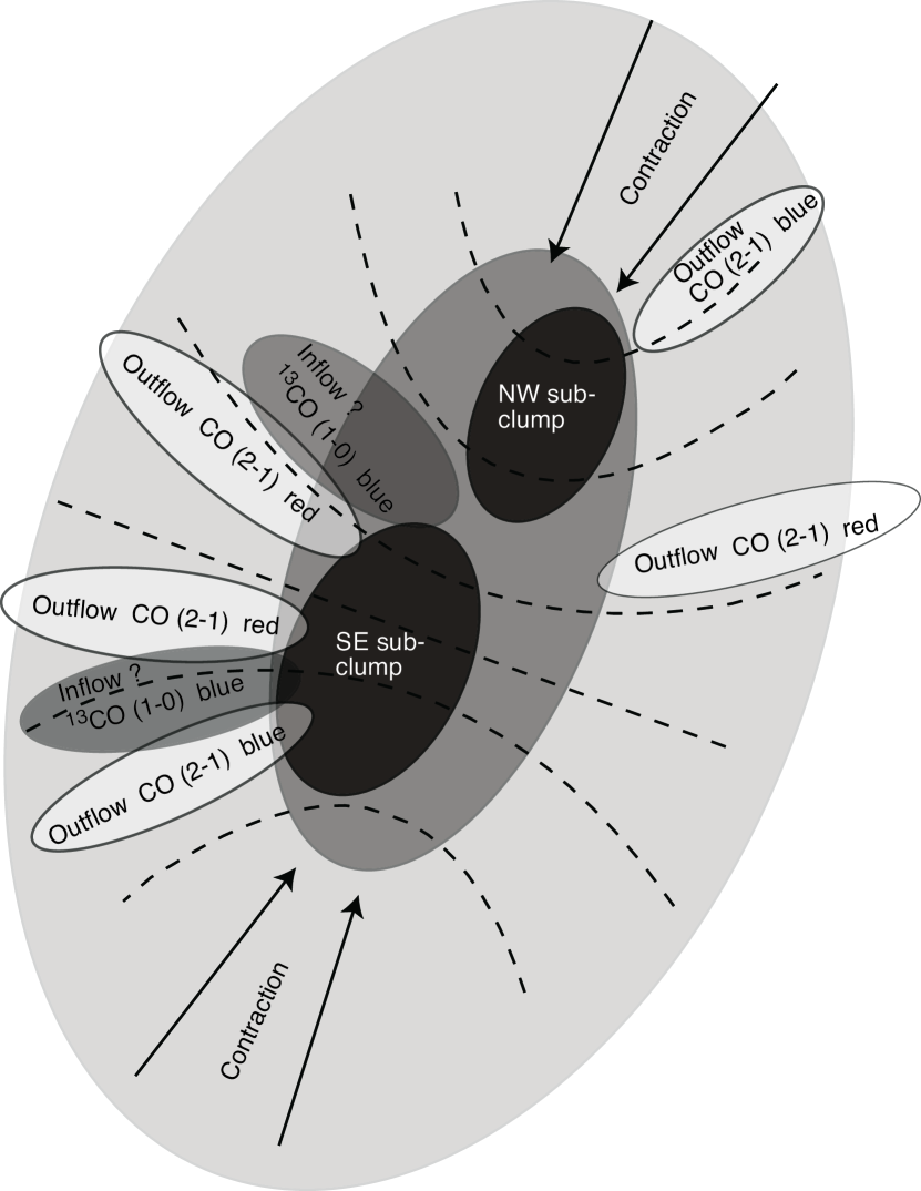
Figure 10: The schematic drawing of the Serpens cloud core. The pinched or hourglass-shaped magnetic field pattern suggests that the magnetic field lines are dragged along with the contracting gas toward the center of the cluster.

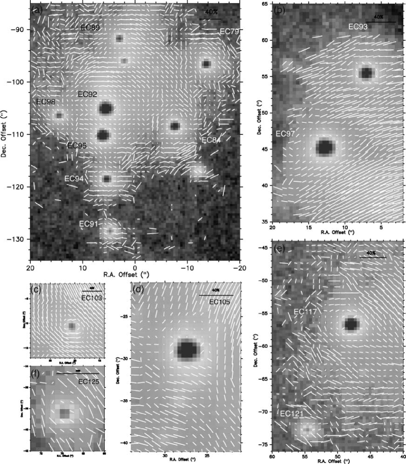
Figure 11: $K$s polarization vector maps of the nebulosities associated with YSOs in the SVS 4 cluster and the central region of the Serpens cloud core, superposed on the total intensity images in the logarithmic scale. The vectors were shown every 2 pixels. The reference position of offset is $(\alpha,{\mathit{\delta}})_{\rm J2000}$ =(18:29:57.39, +01:14:36.2). North is at the top and east is to the left. 40% vector is shown at each panel. YSOs with reflection nebulae are marked.

Toward the four areas, the H₂ column densities from C¹⁸O could be estimated to be $\sim 6\times 10^{22}$ cm^-2 from Figure 11 of Olmi & Testi (2002). Adopting the approximate C¹⁸O extent of $\sim$12′($\sim$0.9 pc at d$\sim$260 pc; Figure 2 of Olmi & Testi, 2002) as the depth of these area, we obtain the H₂ densities of $\sim 2.1\times 10^{4}$ cm^-3. From Figure 10 of Olmi & Testi (2002), the C¹⁸O velocity widths could be estimated to be $\sim$1.6–1.8 km s^-1 toward the SE and NE corners, and $\sim$1.8–2.0 km s^-1 toward the area next to the NE corner. Toward the SW corner with a complex distribution of velocity width, the velocity width may be $\sim$1–2 km s^-1. Using a mean molecular mass, $\mu$, of 2.3 and these values to derive the velocity dispersions, we roughly evaluated the magnetic field strength of the plane-of-the-sky of $B_{\parallel}\sim$160–180 $\mu$G toward the SE corner, $\sim$150–160 $\mu$G toward the NE corner, and $\sim$180–200 $\mu$G toward the area next to the NE corner. Although $\sim$50–90 $\mu$G can be evaluated toward the SW corner, this value might be more uncertain than those toward the other areas due to the larger uncertainty of the velocity width. The magnetic field strength evaluated here is higher than those measured around dark cloud complexes and prestellar cores, a few 10 $\mu$G (e.g., Alves et al., 2008; Kandori et al., 2009, respectively), but smaller than those around HII regions, a few mG (e.g., Houde, 2004) and of a protostellar envelope, a few mG (Girart et al., 2006).

Recently, Houde et al. (2009) showed how the signal integration through the thickness of the cloud and the area of the telescope beam affects on the measured angular dispersion and apply their results to OMC-1. Based on their estimated number (N=21) of the independent turbulent cells contained within the column probed by the telescope beam, they found that a correction factor of $1/\sqrt{N}\sim 0.2$ is applicable to OMC-1. In our case, although the area of the telescope beam is negligibly small due to the point sources, the thickness of the cloud should be taken into account and the correction factor should be somewhat smaller than $\sim 0.5$. If we assume that the effect of the cloud thickness is similar to that of OMC-1, we obtain $N\sim 11$, suggesting a factor of $\sim 0.3$. Adopting this factor of $\sim 0.3$, the above estimated values are reduced by a factor of $\sim 0.6$ and $B_{\parallel}\sim 100$ may be appropriate for the ambient region of the Serpens cloud core, except the SW corner.

Here, we roughly derive the mass to magnetic flux ratio $M_{\rm cloud}/\Psi$ using our estimated value of $B\sim$100 $\mu$G, and compare it with the critical value for a magnetic stability of the cloud, ($M_{\rm cloud}/\Psi$)${}_{\rm critical}=(4\pi^{2}G)^{-1/2}$ (Nakano & Nakamura, 1978). With a formula $M_{\rm cloud}/\Psi=(\pi R^{2}\mu m_{\rm H}N)/(\pi R^{2}B)=\mu m_{\rm H}N/B$ and the H₂ column density $N\sim 6\times 10^{22}$ cm^-2 where we estimated $B$, we derive $M_{\rm cloud}/\Psi\sim 3.8\times(M_{\rm cloud}/\Psi)_{\rm critical}$, where $R$ is a radius of the cloud and $m_{\rm H}$ is the mass of a hydrogen atom. Although this derived value is slightly larger than the critical value, $M_{\rm cloud}/\Psi$ could be much larger in the inner region of the cloud core because the column density of the inner region is much higher than those where we estimated $B$, but the magnetic field may be slightly larger than that we estimated in the ambient region, judged from the slowly curved shape of the magnetic field. We note that the adopted strength of the magnetic field is that estimated for the projection of the magnetic field in the plane of the sky, suggesting a slightly smaller $M_{\rm cloud}/\Psi$ than the estimated one. These imply that the ambient region is marginally supercritical, while the inner region is supercritical. This situation is considered to be quite consistent with the hourglass shape of the magnetic field and with the cluster formation within the sub-clumps.

It is interesting to examine whether the magnetic field can maintain the outflow collimation along the magnetic field in the ambient region of the sub-clumps, i.e., whether the magnetic field can guide the outflows. The magnetic pressure, $P_{B}=B^{2}/8\pi$, is calculated to be $\sim$ 4 $\times$10^-10 dyn, adopting $B\sim 100\mu$G. Assuming the average density and velocity width due to turbulence for the outflow to be $3\times 10^{3}$ cm^-3, which would be consistent with the optically thin condition of the high velocity gas (White et al., 1995), and 3 km s^-1, which is larger than the C¹⁸O velocity width by a factor of $\sim$1.5–2.0, we obtain the turbulent pressure, $P_{\rm turb}=\rho\sigma_{\rm turb}^{2}$, of $\sim 2\times$10^-10 dyn. Taking into account the fact that the adopted strength of the magnetic field is that estimated for the projection and that $P_{B}$ is proportional to $B^{2}$, these estimates imply that the magnetic field can guide the outflows in the ambient region of the Serpen cloud core.

4.4 Comparison with outflow-driven turbulence model for cluster formation

From our analysis, the magnetic field seems to be important in considering the cloud stability that is related to star formation or cluster formation and the feed back from the star formation activity, such as outflows.

The hourglass-shaped magnetic field suggests that the Serpens cloud core first contracted along the straight magnetic field to be a filament or elongated cloud, which is perpendicular to the magnetic field, and that then the central part contracted cross the magnetic field due to the high density in the central region of the cloud core. This situation is very similar to the contraction of the low-mass core that is penetrated by the uniform magnetic field (e,g., Girart et al., 2006; Kandori et al., 2009). In addition, there might exist the cloud rotation, of which axis agrees with that of the hourglass-shaped magnetic field. It was reported that many small-scale outflows spread to or penetrate the NW and SW sub-clupms(e.g., Herbst et al., 1997; Hodapp, 1999; Davis et al., 1999; Ziener & Eislöffel, 1999), and the ambient, larger-scale outflows (filaments) seem to run along the magnetic field as shown above (Davis et al., 1999; Narayanan et al., 2002). Moreover, it is possible that the blue-shifted ¹³CO ($1-0$) features just outside CLS 1, which correspond to the red-shifted CO ($2-1$) outflows, are inflows from the ambient to the central part of the SE sub-clump. Considering these altogether, we may have to take into account the magnetic field, outflows, inflows, cloud rotation, and contraction as well as the turbulence of the molecular gas in the cluster formation process of the Serpens cloud core (see Figure 10).

The structures mentioned above seem to be in good agreement with the outflow-driven turbulence modelof Li & Nakamura (2006) and Nakamura & Li (2007) who performed 3D MHD simulation of cluster formation takinginto accout the effect of protostellar outflows. They demonstrated that protostellar outflows can generate supersonic turbulence in pc-scale cluster forming clumps like the Serpens cloud core. One of the important characteristics of outflow-driven turbulence is that gravitational infall motions almost balance the outward motions driven by outflows, creating very complicated density and velocity structure (see e.g., Figure 4 of Nakamura & Li, 2007). The resulting quasi-equilibrium state can be maintained through active star formation in the central dense region. In the presence of relatively strong magnetic field, both outflow and inflow motions in the less dense envelope tend to be guided by large scale ordered magnetic field lines. As a result, filamentary strucutures that are roughly converging toward the central dense region appear in the envelope, whereas the density structure tends to be more complicated in the central dense region where self-gravity and turbulence may dominate over the magnetic field. Infall motions detected by ¹³CO ($1-0$) in the Serpens core may correspond to such filamentary structures created by gravitational infall.

To clarify how the outflows and magnetic field affect the dynamical state of the cloud, we assess the force balance in the cloud, following Maury et al. (2009). To prevent the global gravitational contraction, the following pressure gradient is needed to achieve the hydrostatic equilibrium:

$${dP_{\rm grav}\over dr}\simeq-G{M(r)\rho(r)\over r^{2}}\left(1-\alpha^{-2}\right)\ ,$$ (1)

where $M(r)$ is the mass contained within the radius $r$ and we assume that the cloud is spherical. The effect of magnetic field is taken into account by the factor $(1-\alpha^{-2})$ and $\alpha$ is the mass-to-magnetic flux ratio normalized to the critical value and is approximated as

$$\alpha\simeq{2\pi G^{1/2}M/\pi r^{2}\over B}$$ (2)

(e.g., Nakano, 1998).

Assuming the density profile of $\rho\propto r^{-2}$, the pressure needed to support the cloud against the gravity is estimated to be

$$P_{\rm grav}\simeq{GM(R)^{2}\over 8\pi R^{4}}\left(1-\alpha^{-2}\right)\ .$$ (3)

The force needed to balance the gravitational force is thus evaluated to be

$$F_{\rm grav}\simeq 4\pi R^{2}P_{\rm grav}(R)={GM(R)^{2}\over 2R^{2}}\left(1-\alpha^{-2}\right)\ .$$ (4)

Adopting $M(R)=210M_{\odot}$, $R=0.46$ pc (Olmi & Testi, 2002), $B=100\mu$G and $\alpha=3.8$, $F_{\rm grav}$ can be estimated to be $\sim 4.3\times 10^{-4}M_{\odot}$ km s^-1 yr^-1. The moderately strong magnetic field of $\alpha=3.8$ can reduce the gravitational force by $\sim$7%. We note that we rescaled the cloud mass and radius derived from Olmi & Testi (2002) by assumingthe distance to the cloud of 260 pc. Hereafter, we also use other values rescaled for this distance.

On the basis of the CO ($J=2-1$) observations, Davis et al. (1999) detected many powerful CO outflows in this cloud, and derived the physical properties of the outflows. From their analysis, we can evaluate the total force exerted by the outflows in this region as

$$F_{\rm outflow}\simeq{p_{\rm outflow}\over t_{\rm dyn}}\sim{8.7\textendash 17.5M_{\odot}{\rm km\ s}^{-1}\over 2.5\times 10^{4}{\rm yr}}\sim(3.4\textendash 7.0)\times 10^{-4}M_{\odot}\ {\rm km\ s^{-1}\ yr^{-1}}\$$ (5)

where $p_{\rm outflow}$ is the total outflow momentum, and $t_{\rm dyn}$ is the representative dynamical time of the outflows. The force due to the outflows, $F_{\rm outflow}$, is comparable to or somewhat larger than the force needed to stop the global gravitational collapse, $F_{\rm grav}$, suggesting that the outflows play a crucial role in the cloud dynamics. This result, however, apparently contradicts that of Olmi & Testi (2002) who suggested that the cloud may be undergoing a global contraction, although the further justification is needed to confirm their interpretation. This apparent inconsistency may come from our assumption of the spherical cloud. Since the relatively strong magnetic field associated with the cloud can guide the large scale outflow motions along the global magnetic field as discussed in the previous subsection, the force exerted by the outflows is expected to be weak along the cross-field direction. As a result, the cloud may be able to contract along the cross-field direction. For the Serpens core, both the magnetic field and the outflows are likely to control the cloud dynamics.

The outflows are also expected to be the major source for generating supersonic turbulence in the Serpens core. From the physical quantities of the outflows measured by Davis et al. (1999), we can evaluate the total energy injection rate due to the outflows in this region as

$${dE_{\rm outflow}\over dt}\simeq{E_{\rm outflow}\over t_{\rm dyn}}\sim{(12.7\textendash 48.3)\ {\rm J}\over 2.5\times 10^{4}\ {\rm yr}}\sim(0.5\textendash 2)L_{\odot}\ .$$ (6)

where $E_{\rm outflow}$ is the total outflow energy. The energy dissipation rate of supersonic turbulence is obtained by Mac Low (1999) as

$${dE_{\rm turb}\over dt}=f{1/2M\Delta V^{2}\over\lambda_{d}/\Delta V}$$ (7)

where $f(=0.34)$ is the non-dimensional constant determined from the numerical simulations, and $M$ is the cloud mass, and $\Delta V$ is the 1D FWHM velocity width. The driving scale of the turbulence $\lambda_{d}$ is estimated to be $\lambda_{d}\sim 0.4$ pc for the outflow-driven turbulence (Matzner, 2007; Nakamura & Li, 2007). The energy dissipation rate of the turbulence can be estimated to be $\sim 0.12L_{\sun}$, where the FWHM velocity width of about 2 km s^-1 is adopted (Olmi & Testi, 2002). This energy dissipation rate is somewhat smaller than the outflow energy input rate. In the Serpens cloud core, the relatively strong magnetic field tends to guide the outflows and therefore the significant amount of the outflow energy might escape away from the cloud along the magnetic field, as inferred from the magnetic field and outflow structures discussed above. In any case, the outflows seem to have sufficient energy to power supersonic turbulence in this region and the magnetic field seems to play an important role in the escape of the outflow energy from the cloud. These characteristics appear to be in agreement with the the outflow-driven turbulence model for cluster formation, and imply the importance of the magnetic field for the continuous star formation in the central region of the Serpens cloud core under the condition where the outflow energy injection rate is high. The Serpens cloud core is expected to be one of the good examples of the outflow-driven turbulence model for cluster formation.

4.5 Summary

We have conducted deep and wide ($\sim$7$\farcm$7 $\times$ 7$\farcm$7) $JHK_{\rm s}$ imaging polarimetry of the Serpens cloud core. The main findings are as follows:

1. The central part of the infrared reflection nebula is illuminated mainly by two sources; the north by SVS 2 (SRN) and the south by SVS 20 with two centrosymmetric patterns. The characteristics of the nebula are consistent with those reported in the previous infrared polarimetric works. Detailed inspection enabled us to find 24 YSOs associated with IR nebulae, in addition to SVS 2 and SVS 20.

2. Polarization of NIR point sources was measured and those sources, except YSOs, have an upper limit of polarization degree similar to that of the nearby star forming regions. It is consistent with the dichroic origin, i.e., the polarization vectors of the near-IR point sources could indicate the direction of the averaged local magnetic field.

3. The polarization vectors suggest a clear hourglass shape. We have made a model fitting of this shape with a parabolic function and found that the symmetry axis ($\theta_{\rm PA}\sim$70°) of the hourglass magnetic field is nearly perpendicular to the elongation ($\sim 150\arcdeg$) of the bright parts of C¹⁸O ($J=1-0$) or submillimeter continuum emissions, i.e., the alignment direction of NW and SE sub-clumps. The submillimeter continuum filaments and CO outflow lobes, which protrude from these sub-clumps, seems to run along the best-fit magnetic field in the ambient region and some ¹³CO velocity features also seem to be along the magnetic field.

4. The evaluation of the magnetic field strength has been done with the CF method toward the ambient area of the Serpens cloud core, taking into account the recent study on the signal integration effect for the dispersion component of the magnetic field. The mass to magnetic flux ratio was estimated with the evaluated magnetic field strength of $\sim 100\mu$G and the parameters of the previous C¹⁸O ($J=1-0$) observations, and found to be slightly larger than the critical value of magnetic instability in the the ambient area. This suggests a possibility that the central region is magnetically unstable, which is consistent with the fact that star formation is actively taking place in the central region. We estimated the magnetic pressure and the turbulent pressure of the outflow using the evaluated magnetic field strength and possible turbulent parameters, and found that the magnetic pressure could be high enough to guide the outflows in the ambient region.

5. The bright part of C¹⁸O ($J=1-0$), submillimeter continuum cores as well as many class 0/I objects are located just toward the constriction region of the hourglass-shaped magnetic field. These suggest that the Serpens cloud core first contracted along the magnetic field to be an elongated cloud and that then the central part contracted cross the magnetic field due to the high density in the central region of the cloud core.

6. Comparisons of the best-fit magnetic field with the previous observations of molecular gas and large-scale outflows suggest a possibility that the cloud dynamics is controlled by the magnetic field, protostellar outflows and gravitational inflows. In addition, the outflow energy injection rate appears to be the same as or larger than the dissipation rate of the turbulent energy in this cloud, indicating that the outflows are the main source of turbulence and that the magnetic field plays an important role both in allowing the outflow energy to escape from the central region of the cloud core and enabling the gravitational inflows from the ambient region to the central region. These characteristics appear to be in good agreement with the outflow-driven turbulence model for cluster formation and imply the importance of the magnetic field to continuous star formation in the center region.

Appendix A Identification of YSOs with NIR reflection nebulae toward the central region of the Serpens cloud core

Except isolated YSOs that are on the periphery of the central region, it is not easy to examine whether YSOs have reflection nebulae locally illuminated by themselves only with the binned map of the $K$ s polarization vectors (Figure 3), due to the contamination of light from the strong sources or nearby sources. We constructed the highest resolution maps without binning for the sources suffering from the contamination of SVS 2, SVS 20 and the members of the SVS 4 cluster, and tried to identify which sources are associated with reflection nebulae. In Figure 11, we show the polarization vector maps only for YSOs that we have identified as those having reflection nebulae. For EC 94, EC 98, and EC 121, although the vector map quality/resolution is not always good enough for the robust identification, we concluded, taking account the weak emission around these sources, that they probably have reflection nebulae.

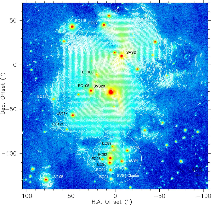
Figure 3: $K$s polarization vector map of the central region of the Serpens cloud core, superposed on the total intensity images in the logarithmic scale. The vectors were made by 3$\times$3 pixel binning. The area of the image is $220\arcsec\times 220\arcsec.$ The reference position of offset is $(\alpha,{\mathit{\delta}})_{\rm J2000}$ =(18:29:57.39, +01:14:36.2). North is at the top and east is to the left. 40% vector is shown near the bottom right corner. The young stellar objects with reflection nebulae are marked. The SVS 4 cluster is shown by the circle.

Figure 5: Top: polarization degrees at $H$ versus $H-K$s color for sources having the $H$-band polarization errors of $<0.3\%$. Bottom: polarization P.A.s at $H$ versus $H-K$ color for sources having $P/{\mathit{\Delta}}P>3$ and $P<6.2(H-Ks)$.

Figure 7: $H$-band measured polarization vectors (solid bars) for point sources having $P/{\mathit{\Delta}}P>3$ and $P<6.2(H-K{\rm s})$ and their best-fit polarization (magnetic field) vectors (dashed bars) with a parabolic function ($x=g+gCy^{2}$), where the $x$ is the distance from the parabolic magnetic field axis of symmetry having the coefficient of $y^{2}$ of $C=(7.00\pm 0.39)\times 10^{-6}$ pixel^-2 and the symmetry center of the magnetic field is $(x,y)_{\rm center}=(646.0\pm 11.3,384.0\pm 9.1$), which corresponds to $(\alpha,\delta)_{\rm J2000}$ =(18:29:54.9, +01:13:13), on the axis of symmetry that is tilted at $\theta_{\rm PA}=70.01\arcdeg\pm 0.77\arcdeg$. $10\%$ vector is shown near the upper right corner. The area of the figure is $\sim 8\farcm 4\times 8\farcm 5$, nearly same as that of Fig. 6. YSOs identified by the Spitzer space telescope are marked by circles, and these YSOs are not used for the fitting. In four areas enclosed by dashed lines, additional fitting with one-parameter ($C$) was done (see text).

Table 1: YSOs with NIR nebulae toward the central region.

YSO Name	$K$s	Source	SSTc2dJ	ISO	Other Name
(Spitzer ID )	(mag)	Class	ID	ID
EC79 (80)	11.5	2	18295655+0112595	304	GCNM84/STGM12
SVS2 (9)	9.3	0/1	18295687+0114465	307	EC82/GCNM87/CK3/STGM22
EC84 (85)	11.1	2	18295696+0112477	309	GCNM90/STGM11
EC89 (12)	12.0	0/1	18295766+0113046	(312)	GCNM97/STGM13
SVS20S/N (35)	7.1	FS	18295772+0114057	314	EC90/GCNM98/CK1/STGM18
EC91 (70)	13.0	2	18295780+0112279	320	GCNM101
EC92 (2)	10.5	0/1	18295783+0112514	(317)	GCNM104
EC93 (83)	10.8	2	18295780+0115318	319	GCNM100/STGM25/CK12
EC94 (37)	11.7	FS	18295784+0112378	318	GCNM102
EC95 (105)	10.0	2	18295789+0112462	(317)	GCNM103
EC97 (27)	9.9	FS	18295819+0115218	321	GCNM106/CK4/STGM24
EC98 (165)	12.3	TD	18295844+0112501	322	GCNM110
EC103 (4)	11.8	0/1	18295877+0114262	326	GCNM112/STGM20/K2_5
EC105 (59)	9.5	2	18295923+0114077	328	GCNM119/CK8/STGM19/K2_6
EC117 (216)	10.1	3	18300065+0113402	338	GCNM135/CK6
EC118 (158)	9.0	TD	18300061+0115204	337	GCNM136/CK2
EC121 (30)	13.2	FS	18300109+0113244	341	GCNM142
EC125 (1)	13.4	0/1	18300208+0113589	345	GCNM154/CK7/STGM16
EC129 (10)	9.9	0/1	18300273+0112282	347	GCNM160/STGM10

Table 2: YSOs with NIR nebulae toward the NW region.

YSO Name	$K$s	Source	SSTc2dJ	ISO	Other Name
(Spitzer ID )	(mag)	Class	ID	ID
DEOS/S68Nd (11)	14.9	0/1	18294913+0116198	250	knot c/K4_5/WMW11
S68Nc	$\cdots$	(0/1)	$\cdots$	$\cdots$	subknot a3/knot a
SMM1-FIRS1	$\cdots$	$\cdots$	18294963+0115219	258a	GCNM23/WMW114/VLA7
EC53/SMM5 (24)	11.3	0/1	18295114+0116406	265	STGM27/WMW24
EC67 (81)	9.6	2	18295359+0117018	283	GCNM60/STGM29/WMW81
EC38/S68Nb (7)	12.7	0/1	18294957+0117060	254	WMW7
SMM10-IR (21)	17.7	0/1	18295219+0115478	270	WMW21

References

- Allen et al. (2007) Allen, L. E., et al. 2007, in Protostars and Planets V, ed. B. Reipurth, D. Jewitt & K. Keil (Univ. Arizona Press), 361
- Alves et al. (2008) Alves, F. O., Franco, G. A. P., & Girart, J. M. 2008, A&A, 486, L13 & Bailey, J. A., 1991, ApJ, 375, 611
- Chandrasekhar & Fermi (1953) Chandrasekhar, S., & Fermi, E. 1953, ApJ, 118, 113
- Curiel et al. (1996) Curiel, S., Rodoriguez, L., Gomez, J. F., Torrelles, J. M., Ho, P. T. P., & Eiroa, C. 1996, ApJ, 456, 677
- Eiroa et al. (2008) Eiroa, C., Djupvik, A. A. & Casali, M. M. 2008, in ASP Conf. Ser. Handbook of Star Forming Regions, ed. B. Reipurth (San Francisco: ASP), 693
- Eiroa & Casali (1989) Eiroa, C., & Casali, M. M. 1989, A&A, 223, L17
- Enoch et al. (2007) Enoch, M. L., Glenn, J., Evans II, N. J. et al. 2007, ApJ, 666, 982
- Davis et al. (1999) Davis, C. J., Matthews, H. E., Ray, T. et al. 1999, MNRAS, 309, 141
- Girart et al. (2006) Girart, J. M., Rao, R., & Marrone, D. P. , Science, 313, 812
- Gomez de Castro et al. (1988) Gomez de Castro, A. L., Eiroa, C., & Lenzen, R. et al. 1999, A&A, 201, 299
- Harvey et al. (2006) Harvey, P., Chapman, N., Lai, S.-P. et al. 2006, ApJ, 644, 307
- Harvey et al. (2007) Harvey, P., Merin, B., Huard, T. L. et al. 2007, ApJ, 663, 1149
- Heitsch et al. (2001) Heitsch, F., Zweibel, E. G., Mac Low, M.-M., Li, P., & Norman, M. L. 2001, ApJ, 561, 800
- Herbst et al. (1997) Herbst, T. M., Beckwith, S. V. W., & Robbert, M. 1997, ApJ, 486, L59
- Hodapp (1999) Hodapp, K. W. 1999, AJ, 118, 1338
- Houde et al. (2004) Houde, M., Dowell, C. D., Hildebrand, R. H., Dorson, J. L., Vailiancour, J. E., Phillips, T. G., Peng, R., & Bastien, P. 2004 ApJ, 604, 717
- Houde (2004) Houde, M. 2004 ApJ, 616, L111
- Houde et al. (2009) Houde, M., Vaillancourt, J. E., Hildebrand, R. H., Chitsazzadeh, S., & Kirby, L. 2009 ApJ, 706, 1504
- Huard et al. (1997) Huard, T. L., Weintraub, D. A., &Kastner, J. H. 1997, 290, 598
- Ikeda et al. (2007) Ikeda, N., Sunada, K., & Kitamura, Y. 2007, ApJ, 665, 1194
- Kaas et al. (2004) Kaas, A. A., Olofsson, G., Bontemps, S. et al. 2004, A&A, 421, 623
- Kandori et al. (2006) Kandori, R., et al. 2006, Proc. SPIE, 6269
- Kandori et al. (2009) Kandori, R., Tamura, M., Tatematsu, K., Kusakabe, N., Nakajima, Y., & IRSF/SIRPOL group 2009, in Cosmic Magnetic Fields: From Planets, to Stars and Galaxies, Proc. of IAU Sympo., No. 259, ed. K.G. Strassmeier, A.G. Kosovichev, & J.E. Beckman, in press
- King et al. (1983) King, D. J., Scarrot, S. M., & Taylor, K. N. R. 1983, MNRAS, 202, 1087
- Kirby (2009) Kirby, L. 2009, ApJ, 694, 1056
- Klessen et al. (1998) Klessen, R., Burkert, A., & Bate, M. R. 1998, ApJ, 501, L205
- Kusakabe et al. (2008) Kusakabe, N., Tamura, M., Kandori, R., Hashimoto, J., Nakajima, Y., Nagata, T., Nagayama, T., Hough, J., & Lucas, R. 2008, AJ, 136, 621
- Kudoh & Basu (2003) Kudoh, T., & Basu, S. 2003, ApJ, 595, 842
- Lada & Lada (2003) Lada, C., & Lada, E. A. 2003, ARA&A, 41, 57
- Lai et al. (2002) Lai, S.-P., Crutcher, R. M., Girart, J. M., & Rao, P. 2002, ApJ, 566, 925
- Li & Nakamura (2006) Li, Z.-Y., & Nakamura, F. 2007, ApJ, 640, L187
- Matzner (2007) Matzner, C. D. 2007, ApJ, 659, 1394
- Mac Low (1999) Mac Low, M. -M. 1999, ApJ, 524, 169
- Maury et al. (2009) Maury, A. J., André, P., & Li, Z.-Y. 2009, A&A, 499, 175
- McKee & Ostriker (2007) McKee, C. F., & Ostriker, E. C. 2007, ARA&A, 45, 565
- McMullin et al. (2000) McMullin, J. P., Mundy, L. G., Blake, G. A. 2000, ApJ, 536, 845
- Nagashima et al. (1999) Nagashima, C., et al. 999, in Star Formation 1999, ed. T. Nakamoto (Nobeyama: Nobeyama Radio Observatory), 397
- Nakamura & Li (2007) Nakamura, F., & Li, Z.-Y.. 2007, ApJ, 662, 395
- Nagayama et al. (2003) Nagayama, T., et al. 2003, Proc. SPIE, 4841, 459
- Nakano & Nakamura (1978) Nakano, T., & Nakamura, T. 1978, PASJ, 30, 671
- Nakano (1998) Nakano, T. 1998, ApJ, 494, 587
- Narayanan et al. (2002) Narayanan, G., Moriarty-Schieven, G., Walker, C. K., & Butner, H. M. 2002, 565, 319
- Olmi & Testi (2002) Olmi, L. , & Testi, L. 2002, A&A, 392, 1053
- Ostriker et al. (2001) Ostriker, E. C., Stone, J. M., & Gammie, C. F. 2001, ApJ, 546, 980
- Reid & Wilson (2006) Reid, M. A., & Wilson, C. D. 2006, ApJ, 650, 970
- Padoan et al. (2001) Padoan, P., Goodman, A. A., Draine, B. T., Juvela, M., Nordlund, Å., & Rögnvaldsson, Ö., E. 2001, ApJ, 559, 1005
- Pontoppidan & Dullemond (2005) Pontoppidan, K. M., & Dullemond, C. P. 2002, A&A, 392, 1053
- Schleuning (1998) Schleuning, D. A. 1998, ApJ, 493, 811
- Skrutskie et al. (2006) Skrutskie, M. F. et al. 2006, AJ, 131, 1163
- Sogawa et al. (1997) Sogawa, H, Tamura, M., Gatley, I. & Merrill, M. 1997, AJ, 113, 1057
- Straižys et al. (2003) Straižys, V., Černis, K., & Bartašiute, K. M. 1976, AJ, 81, 638
- Strom et al. (1976) Strom, S. E., Vrba, F. J., & Strom, K. M. 1976, AJ, 81, 638
- Testi & Sargent (1998) Testi, L., & Sargent, A. I. 1998, ApJ, 508, L91
- Testi et al. (2000) Testi, L., Sargent, A. I., Olmmi, L. & Onell, J. S. 2000, ApJ, 540, L53
- Warren-Smith et al. (1987) Warren-Smith, R. F., Draper, P. W., & Scarrott, S. 1987, MNRAS, 227, 749
- White et al. (1995) White, G. J., Casali, M. M., & Eiroa, C. 1995, A&A, 298, 594
- Whittet et al. (2008) Whittet, D. C. B., Hough, J. H., Lazarian, A., & Hoang, T. 2008, ApJ, 674, 304
- Williams & Myers (2000) Williams, J., & Myers, P. C. 2000, ApJ, 537, 891
- Winston et al. (2007) Winston, E., Megeath, S. T., Wolk, S. J. et al. 2007, AJ, 669, 493
- Wardle & Kronberg (1974) Wardle, J. F. C., & Kronberg, P. P. 1974, ApJ, 194, 249
- Wolf-Chae et al. (1998) Wolf-Chae, G. A., Barsony, M., Wootten, H. A., Ward-Thompson, D., Lowrance, P. J., Kastner, J. H., & McMullin, J. P. 1998, ApJ, 501, L193
- Ziener & Eislöffel (1999) Ziener, R., & Eislöffel, J. 1995, A&A, 347, 565