Faster Algorithms for Semi-Matching Problems

Abstract

We consider the problem of finding semi-matching in bipartite graphs which is also extensively studied under various names in the scheduling literature. We give faster algorithms for both weighted and unweighted cases.

For the weighted case, we give an $O(nm\log n)$-time algorithm, where $n$ is the number of vertices and $m$ is the number of edges, by exploiting the geometric structure of the problem. This improves the classical $O(n^{3})$-time algorithms by Horn [Operations Research 1973] and Bruno, Coffman and Sethi [Communications of the ACM 1974].

For the unweighted case, the bound can be improved even further. We give a simple divide-and-conquer algorithm which runs in $O(\sqrt{n}m\log n)$ time, improving two previous $O(nm)$-time algorithms by Abraham [MSc thesis, University of Glasgow 2003] and Harvey, Ladner, Lovász and Tamir [WADS 2003 and Journal of Algorithms 2006]. We also extend this algorithm to solve the Balanced Edge Cover problem in $O(\sqrt{n}m\log n)$ time, improving the previous $O(nm)$-time algorithm by Harada, Ono, Sadakane and Yamashita [ISAAC 2008].

1 Introduction

In this paper, we consider a relaxation of the maximum bipartite matching problem called semi-matching problem, in both weighted and unweighted cases. This problem has been previously studied in the scheduling literature under different names, mostly known as (non-preemptive) scheduling independent jobs on unrelated machines to minimize flow time, or $R||\sum C_{j}$ in the standard scheduling notation [3, 26, 2].

Informally, the problem can be explained by the following off-line load balancing scenario. We are given a set of jobs and a set of machines. Each machine can process one job at a time and it takes different amounts of time to process different jobs. Each job also requires different processing times if it is processed by different machines. One natural goal is to have all jobs processed with the minimum total completion time, or total flow time, which is the summation of the duration each job has to wait until it is finished. Observe that if the assignment is known, the order each machine processes its assigned jobs is clear: It processes jobs in an increasing order of the processing time.

To be precise, the semi-matching problem is as follows. Let $G=(U\cup V,E)$ be a weighted bipartite graph, where $U$ is a set of jobs and $V$ is a set of machines. For any edge $uv$, let $w_{uv}$ be its weight. Each weight of an edge $uv$ indicates time it takes $v$ to process $u$. Through out this paper, let $n$ denote the number of vertices and $m$ denote the number of edges in $G$. A set $M\subseteq E$ is a semi-matching if each job $u\in U$ is incident with exactly one edge in $M$. For any semi-matching $M$, we define the cost of $M$, denoted by $\mathrm{cost}(M)$, as follows. First, for any machine $v\in V$, its cost with respect to a semi-matching $M$ is

$$\mathrm{cost}_{M}(v)=(w_{1})+(w_{1}+w_{2})+\ldots+(w_{1}+\ldots+w_{\mathrm{deg}_{M}(v)})=\sum_{i=1}^{\mathrm{deg}_{M}(v)}(\mathrm{deg}_{M}(v)-i+1)\cdot w_{i}$$

where $\mathrm{deg}_{M}(v)$ is the degree of $v$ in $M$ and $w_{1}\leq w_{2}\leq\ldots\leq w_{\mathrm{deg}_{M}(v)}$ are weights of the edges in $M$ incident with $v$ sorted increasingly. Intuitively, this is the total completion time of jobs assigned to $v$. Note that for the unweighted case (i.e., when $w_{e}=1$ for every edge $e$), the cost of a machine $v$ is simply $\mathrm{deg}_{M}(v)\cdot(\mathrm{deg}_{M}(v)+1)/2$. Now, the cost of the semi-matching $M$ is simply the summation of the cost over all machines:

$$\mathrm{cost}(M)=\sum_{v\in V}\mathrm{cost}_{M}(v).$$

The goal is to find an optimal semi-matching, a semi-matching with minimum cost.

Related works

Although the name “semi-matching” was recently proposed by Harvey, Ladner, Lovász, and Tamir [20], the problem was studied as early as 1970s when an $O(n^{3})$ algorithm was independently developed by Horn in [21] and by Bruno, Coffman and Sethi in [6]. Since then no progress has been made on this problem except on its special cases and variations. For the special case of inclusive set restriction where, for each pair of jobs $u_{1}$ and $u_{2}$, either all neighbors of $u_{1}$ are neighbors of $u_{2}$ or vice versa, a faster algorithm with $O(n^{2})$ running time was given by Spyropoulos and Evans [40]. Many variations of this problem were proved to be NP-hard, including the preemptive version [39], the case when there are deadlines [41], and the case of optimizing total weighted tardiness [29]. The variation where the objective is to minimize $\max_{v\in V}\mathrm{cost}_{M}(v)$ was also considered [32, 25].

The unweighted case of the semi-matching problem also received considerable attention in the past few years. Since it was shown by [20] that an optimal solution of the semi-matching problem is also optimal for the makespan version of the scheduling problem (where one wants to minimize the time the last machine finishes), we mention the results of both problems. The problem was first studied in a special case, called nested case where, for any two jobs, if their sets of neighbors are not disjoint, then one of these sets contains the other set. This case was shown to be solvable in $O(m+n\log n)$ time [36, p.103]. For the general unweighted semi-matching problem, Abraham [1, Section 4.3] and Harvey, Ladner, Lovász and Tamir [20] independently developed two algorithms with $O(nm)$ running time. Lin and Li [28] also gave an $O(n^{3}\log{n})$-time algorithm which is later generalized to a more general cost function [27]. Recently, Lee, Leung and Pinedo [25] showed that the problem can be solved in polynomial time even when there are release times.

Recently after the preliminary version of this paper appeared, the unweighted semi-matching problem has been generalized to the quasi-matching problem by Bokal, Bresar and Jerebic [4]. In this problem, a function $g$ is provided and each vertex $u\in U$ is required to connect to at least $g(u)$ vertices in $v$. Therefore, the semi-matching problem is when $g(u)=1$ for every $u\in U$. They also developed an algorithm for this problem which is a generalization of the Hungarian method and used it to deal with a routing problem in CDMA-based wireless sensor networks.

Galcík, Katrenic and Semanisin [13] very recently showed a nice reduction from the unweighted semi-matching problem to a variant of the maximum bounded-degree semi-matching problem. Their approach resulted in two algorithms. The first algorithm has the same running time as ours while the second algorithm is randomized and has a running time of $O(n^{\omega})$ where $\omega$ is the exponent of the best known matrix multiplication algorithm.

Motivated by the problem of assigning wireless stations (users) to access points, the unweighted semi-matching problem is also generalized to the problem of finding optimal semi-matching with minimum weight where an $O(n^{2}m)$ time algorithm was given [16].

Approximation algorithms and online algorithms for this problem (both weighted and unweighted cases) and the makespan version have also gained a lot of attention over the past few decades and have applications ranging from scheduling in hospital to wireless communication network. (See [26, 48] for the recent surveys.)

Applications

As motivated by Harvey et al. [20], even in an online setting where jobs arrive and depart over time, they may be reassigned from one machine to another cheaply if the algorithm’s running time is significantly faster than the arrival/departure rate. (One example of such case is the Microsoft Active Directory system [15, 20].) The problem also arose from the Video on Demand (VoD) systems where the load of video disks needs to be balanced while data blocks from the disks are retrieved or while serving clients [31, 45]. The problem, if solved in the distributed setting, can be used to construct a load balanced data gathering tree in sensor networks [37, 33]. The same problem also arose in peer-to-peer systems [42, 24, 43].

In this paper, we also consider an “edge cover” version of the problem. In some applications such as sensor networks, there are no jobs and machines but the sensor nodes have to be clustered and each cluster has to pick its own head node to gather information from other nodes in the cluster. Motivated by this, Harada, Ono, Sadakane and Yamashita [17] introduced the balanced edge cover problem where the goal is to find an edge cover (set of edges incident to every vertex) that minimizes the total cost over all vertices. (The cost on each vertex is as previously defined.) They gave an $O(nm)$ algorithm for this problem and claimed that it could be used to solve the semi-matching problem as well. We show that this problem can be efficiently reduced to the semi-matching problem. Thus, our algorithm (for unweighted case) also gives a better bound on the balanced edge cover problem.

Our results and techniques

We consider the semi-matching problem and give a faster algorithm for each of the weighted and unweighted cases. We also extend the algorithm for the unweighted case to solve the balanced edge cover problem.

• Weighted Semi-Matching: (Section 2) We present an $O(nm\log{n})$ algorithm, improving the previous $O(n^{3})$ algorithm by Horn [21] and Bruno et al. [6]. As in the previous results [21, 5, 18], we use the reduction of the weighted semi-matching problem to the weighted bipartite matching problem as a starting point. We, however, only use the structural properties arising from the reduction and do not actually perform the reduction.

• Unweighted Semi-Matching: (Section 3) We give an $O(\sqrt{n}m\log n)$ algorithm, improving the previous $O(nm)$ algorithms by Abraham [1] and Harvey et al. [20]. Our algorithm uses the same reduction to the min-cost flow problem as in [20]. However, instead of canceling one negative cycle in each iteration, our algorithm exploits the structure of the graphs and the cost functions to cancel many negative cycles in a single iteration. This technique can also be generalized to any convex cost function.

• Balanced Edge Cover: (Section 4) We also present a reduction from the balanced edge cover problem to the unweighted semi-matching problem. This leads to an $O(\sqrt{n}m\log n)$ algorithm for the problem, improving the previous $O(nm)$ algorithm by Harada et al. [17]. The main idea is to identify the “center” vertices of all the clusters in the optimal solution. (Note that any balanced edge cover (in fact, any minimal edge cover) clusters the vertices into stars.) Then, we partition the vertices into two sides, center and non-center ones, and apply the semi-matching algorithm on this graph.

2 Weighted semi-matching

In this section, we present an algorithm that finds an optimal weighted semi-matching in $O(nm\log n)$ time.

Overview

Our improvement follows from studying the reduction from the weighted semi-matching problem to the weighted bipartite matching problem considered in the previous works [21, 6, 18] and the Edmonds-Karp-Tomizawa (EKT) algorithm for finding the weighted bipartite matching [9, 47]. We first review these briefly. For more detail, see Appendix A and B.

Reduction

As in [21, 6, 18], we consider the reduction from the semi-matching problem on a bipartite graph $G=(U\cup V,E)$ to the minimum-weight bipartite matching on a graph $\hat{G}$. The reduction is done by exploding the vertices in $V$, i.e., for each vertex $v\in V$, we create $\mathrm{deg}(v)$ vertices, $v^{1},v^{2},\ldots,v^{\mathrm{deg}(v)}$. We also make copies of edges incident to $v$ in the original graph $G$, i.e, for each vertex $u\in U$ such that $uv\in E$, we create edges $uv^{1},uv^{2},\ldots,uv^{\mathrm{deg}(v)}$. For each edge $uv^{i}$ incident to $v^{i}$ in $\hat{G}$, we set its weight to $i$ times its original weight in $G$, i.e, $w_{uv^{i}}=i\cdot w_{uv}$. We denote the set of these vertices by $\hat{V}_{v}$. Thus, we have

$$\hat{G} =(U\cup\hat{V},\hat{E})$$

$$\hat{V} =\{v^{1},v^{2},\ldots,v^{\mathrm{deg}_{G}(v)}:v\in V\}$$

$$\hat{E} =\{uv^{1},uv^{2},\ldots,v^{\mathrm{deg}_{G}(v)}:uv\in E\}$$

$$\hat{w}_{uv^{i}} =i\cdot w_{uv}\quad\forall uv\in E,i\in\{1,2,\ldots,\mathrm{deg}_{G}(v)\}$$

The correctness of this reduction can be seen by replacing the edges incident to $v$ in the semi-matching by the edges incident to $v^{1},v^{2},\ldots$ with weights in decreasing order. For example, in Figure 1(a), edge $u_{1}v_{1}$ and edge $u_{2}v_{1}$ in the semi-matching in $G$ correspond to $u_{1}v_{1}^{1}$ and $u_{2}v_{1}^{2}$ in the matching in $\hat{G}$. The reduction is illustrated in Figure 1(a).

This alone does not give an improvement on the semi-matching problem because the number of edges becomes $O(nm)$. However, we can apply some tricks to improve the running time.

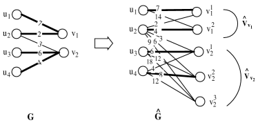
(a) Reduction

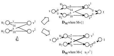
(b) Residual graphs

Figure 1:

EKT algorithm

Our improvement comes from studying the behavior of the EKT algorithm for finding the bipartite matching in $\hat{G}$. The EKT algorithm iteratively increases the cardinality of the matching by one by finding a shortest augmenting path. Such path can be found by applying Dijkstra’s algorithm on the residual graph $D_{M}$ (corresponding to a matching $M$) with a reduced cost, denoted by $\tilde{w}$ as an edge length.

Figure 1(b) shows examples of a residual graph $D_{M}$. The direction of an edge depends on whether it is in the matching or not. The weight of each edge depends on its weight in the original graph and the costs on its end-vertices. We draw an edge of length 0 from $s$ to all vertices in $U_{M}$ and from all vertices in $\hat{V}_{M}$ to $t$, where $U_{M}$ and $\hat{V}_{M}$ are the sets of unmatched vertices in $U$ and $\hat{V}$, respectively. We want to find the shortest path from $s$ to $t$ or, equivalently, from $U_{M}$ to $\hat{V}_{M}$.

The reduced cost is computed from the potentials on the vertices, which can be found as in Algorithm 2.1.

Algorithm 2.1 EKT Algorithm $(\hat{G},w)$

1:  Let $M=\emptyset$.

2:  For every node $v$, let $p(v)=0$. ($p(v)$ is a potential on $v$.)

3:  repeat

4:      Let $\tilde{w}_{uv}=w_{uv}+p(u)-p(v)$ for every edge $uv$. ($\tilde{w}_{uv}$ is a reduced cost of an edge $uv$.)

5:     For every node $v$, compute the distance $d(v)$ which is the distance from $U_{M}$ (the set of unmatched vertices in $U$) to $v$ in $D_{M}$. (Recall that the length of edges in $D_{M}$ is $\tilde{w}$.)

6:     Let $P$ be the shortest $U_{M}$-$\hat{V}_{M}$ path in $D_{M}$.

7:     Update the potential $p(u)$ to $d(u)$ for every vertex $u\in U\cup(\hat{V}\setminus\hat{V}_{M})$.

8:     Augment $M$ along $P$, i.e., $M=P\triangle M$ (where $\triangle$ denotes the symmetric difference operator).

9:  until all vertices in $U$ are matched

10:  return  $M$

Applying EKT algorithm directly leads to an $O(n(n^{\prime}\log n^{\prime}+m^{\prime}))$-time algorithm where $n=|U|$, $n^{\prime}=|U\cup\hat{V}|$ and $m^{\prime}=|\hat{E}|$ are the number of vertices and edges in $\hat{G}$. Since $|\hat{V}|=\Theta(m)$ and $m^{\prime}=O(nm)$, the running time is $O(nm\log n+n^{2}m)$. (We note that this could be brought down to $O(n^{3})$ by applying the result of Kao, Lam, Sung and Ting [22] to reduce the number of participating edges. See Appendix B.) The bottleneck here is the Dijkstra’s algorithm which needs $O(n^{\prime}\log n^{\prime}+m^{\prime})$ time. We now review this algorithm and pinpoint the part that will be sped up.

Dijkstra’s algorithm

Recall that the Dijkstra’s algorithm starts from a source vertex and keeps adding to its shortest path tree a vertex with minimum tentative distance. When a new vertex $v$ is added, the algorithm updates the tentative distance of all vertices outside the tree by relaxing all edges incident to $v$. On an $n^{\prime}$-vertex $m^{\prime}$-edge graph, it takes $O(\log n^{\prime})$ time (using priority queue) to find a new vertex to add to the tree and hence $O(n^{\prime}\log n^{\prime})$ in total. Further, relaxing all edges takes $O(m^{\prime})$ time in total. Recall that in our case, $m^{\prime}=O(nm)$ which is too large. Thus, we wish to reduce the number of edge relaxations to improve the overall running time.

Our approach

We reduce the number of edge relaxation as follows. Suppose that a vertex $u\in U$ is added to the shortest path tree. For every $v\in V$, a neighbor of $u$ in $G$, we relax all edges $uv^{1}$, $uv^{2}$, $\ldots$, $uv^{i}$ in $\hat{G}$ at the same time. In other words, instead of relaxing $O(nm)$ edges in $\hat{G}$ separately, we group the edges to $m$ groups (according to the edges in $G$) and relax all edges in each group together. We develop a relaxation method that takes $O(\log n)$ time per group. In particular, we design a data structure $H_{v}$, for each vertex $v\in V$, that supports the following operations.

• Relax($uv$, $H_{v}$): This operation works as if it relaxes edges $uv^{1}$, $uv^{2}$, $\ldots$

• AccessMin($H_{v}$): This operation returns a vertex $v^{i}$ (exploded from $v$) with minimum tentative distance among vertices that are not deleted (by the next operation).

• DeleteMin($H_{v}$): This operation finds $v^{i}$ from AccessMin and then returns and deletes $v^{i}.$

Our main result is that, by exploiting the structure of the problem, one can design $H_{v}$ that supports Relax, AccessMin and DeleteMin in $O(\log n)$, $O(1)$ and $O(\log n)$ respectively. Before showing such result, we note that speeding up Dijkstra’s algorithm and hence EKT algorithm is quite straightforward once we have $H_{v}$: We simply build a binary heap $H$ whose nodes correspond to vertices in an original graph $G$. For each vertex $u\in U$, $H$ keeps track of its tentative distance. For each vertex $v\in V$, $H$ keeps track of its minimum tentative distance returned from $H_{v}$.

Main idea in designing $H_{v}$

Before going into details, we sketch the main idea here. The data structure $H_{v}$ that allows fast “group relaxation” operation can be built because of the following nice structure of the reduction: For each edge $uv$ of weight $w_{uv}$ in $G$, the weights $w_{uv^{1}},w_{uv^{2}},\ldots$ of the corresponding edges in $\hat{G}$ increase linearly (i.e., $w_{uv},2w_{uv},3w_{uv},\ldots$). This enables us to know the order of vertices, among $v^{1},v^{2},\ldots$, that will be added to the shortest path tree. For example, in Figure 1(b), when $M=\emptyset$, we know that, among $v^{1}$ and $v^{2}$, $v^{1}$ will be added to the shortest path tree first as it always has a smaller tentative distance.

However, since the length of edges in $D_{M}$ does not solely depend on the weights of the edges in $\hat{G}$ (in particular, it also depends on potentials on both end-vertices), it is possible (after some iterations of the EKT algorithm) that $v^{1}$ is added to the shortest path tree after $v^{2}$.

Fortunately, due to the way the potential is defined by the EKT algorithm, a similar nice property still holds: Among $v^{1},v^{2},\ldots$ in $D_{M}$ corresponding to $v$ in $G$, if a vertex $v^{k}$, for some $k$, is added to the shortest path tree first, then the vertices on each side of $v^{k}$ have a nice order: Among $v^{1},v^{2},\ldots,v^{k-1}$, the order of vertices added to the shortest path tree is $v^{k-1},v^{k-2},\ldots,v^{2},v^{1}$. Further, among $v^{k+1},v^{k+2},\ldots$, the order of vertices added to the shortest path tree is $v^{k+1},v^{k+2},\ldots$.

This main property, along with a few other observations, allow us to construct the data structure $H_{v}$. In the next section, we show the properties we need and use them to construct $H_{v}$ in the latter section.

2.1 Properties of the tentative distance

Consider any iteration of the EKT algorithm (with a potential function $p$ and a matching $M$). We study the following functions $f_{*_{v}}$ and $g_{*v}$.

Definition 2.1.

For any edge $uv$ from $U$ to $V$ and any integer $1\leq i\leq\mathrm{deg}(v)$, let

$$g_{uv}(i)=d(u)+p(u)+i\cdot w_{uv}\quad\text{and}\quad f_{uv}(i)=g_{uv}(i)-p(v^{i})=d(u)+p(u)-p(v^{i})+i\cdot w_{uv}.$$

For any $v\in V$ and $i\in[\mathrm{deg}(v)]$, define the lower envelope of $f_{uv}$ and $g_{uv}$ over all $u\in U$ as

$$f_{*v}(i)=\min_{u:uv\in E}f_{uv}(i)\quad\quad\text{and}\quad g_{*v}(i)=\min_{u:uv\in E}g_{uv}(i).$$

Our goal is to understand the structure of the function $f_{*v}$ whose values $f_{*v}(1),f_{*v}(2),\ldots$ are tentative distances of $v^{1},v^{2},\ldots$, respectively. The function $g_{*v}$ is simply $f_{*v}$ with the potential of $v$ ignored. We define $g_{*v}$ as it is easier to keep track of since it is a combination of linear functions $g_{uv}$ and therefore piecewise linear. Now we state the key properties that enable us to keep track of $f_{*v}$ efficiently. Recall that $v^{1},v^{2},\ldots$ are the exploded vertices of $v$ (from the reduction).

Proposition 2.2.

Consider a matching $M$ and a potential $p$ at any iteration of the EKT algorithm.

• For any vertex $v\in V$, there exists $\alpha_{v}$ such that $v^{1},\ldots,v^{\alpha_{v}}$ are all matched and $v^{\alpha_{v}+1},\ldots,v^{\mathrm{deg}(v)}$ are all unmatched.

• For any vertex $v\in V$, $g_{*v}$ is a piecewise linear function.

• For any $i$ and any edge $uv\in E$ where $u\in U$ and $v\in V$, $f_{uv}(i)=f_{*v}(i)$ if and only if $g_{uv}(i)=g_{*v}(i)$.

• For any edge $uv\in E$ where $u\in U$ and $v\in V$, let $\alpha_{v}$ be as in (1). There exists an integer $1\leq\gamma_{uv}\leq k$ such that for $i=1,2,\ldots,\gamma_{uv}-1$, $f_{uv}(i)\geq f_{uv}(i+1)$ and for $i=\gamma_{uv},\gamma_{uv}+1,\ldots,\alpha_{v}-1$, $f_{uv}(i)\leq f_{uv}(i+1)$. In other words, $f_{uv}(1),f_{uv}(2),\ldots,f_{uv}(\alpha_{v})$ is a unimodal sequence.

Figure 2(a) and 2(b) show the structure of $g_{*v}$ and $f_{*v}$ according to statement (2) and (4) in the above proposition. By statement (3), the two pictures can be combined as in Figure 2(c): $g_{*v}$ indicates $u$ that makes both $g_{*v}$ and $f_{*v}$ minimum in each interval and one can find $i$ that minimizes $f_{*v}$ in each interval by looking at $\alpha_{v}$ (or near $\alpha_{v}$ in some case).

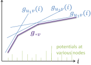
(a) $g_{*v}$ and potential function.

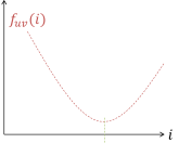
(b) $f_{uv}$ is unimodal.

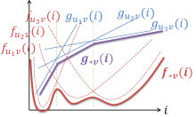
(c) $f_{*v}$ together with $g_{*v}$.

Figure 2: Figures show graphs of potentials, $g_{*v}$, $f_{uv}$ and $f_{*v}$, where $w_{u_{1}v}>w_{u_{2}v}>w_{u_{3}v}>\ldots$. These functions only have value at integer points. For the sake of presentation, these functions are plotted as lines.

Proof.

(1) The first statement follows from the following claim.

Claim 2.3.

For any $i$, if the exploded vertex $v^{i+1}$ of $v$ (in $\hat{V}_{v}$) is matched by $M$, then $v^{i}$ is also matched.

Proof.

The claim follows from the fact that EKT algorithm maintains $M$ so that $M$ is a so-called extreme matching, i.e., $M$ has the minimum weight among matchings of the same size. Suppose that $v^{i+1}$ is matched by $M$ (i.e., $uv^{i+1}\in M$), but $v^{i}$ is not matched. Then we can remove $uv^{i+1}$ from $M$ and add $uv^{i}$ to $M$. The resulting matching will have a cost less than $M$ but have the same cardinality, a contradiction. ∎

(2) To see the second statement, notice that $g_{uv}=d(u)+p(u)+i\cdot w_{uv}$ is linear for a fixed $uv\in E$. Hence, $g_{*v}$ is a lower envelope of a linear function, implying that it is piecewise linear.

(3) To prove the third statement, recall that for any $u$ and any $i$, $f_{uv}(i)=g_{uv}(i)-p(v^{i})$. Therefore, for any $u$, $u^{\prime}$ and $i$, $f_{uv}(i)>f_{u^{\prime}v}(i)$ if and only if $g_{uv}(i)>g_{u^{\prime}v}(i)$. Thus, the third statement follows.

(4) For the fourth claim, we first explain the intuition. First, observe that the function $g_{uv}$ is increasing with rate $w_{uv}$. Moreover, the difference of $f_{uv}(i)$ and $f_{uv}(j)$ is a function of the potential $p(v^{i})$ and $p(v^{j})$ and the multiple of edge weight $(j-i)w_{uv}$. In fact, whether the difference is negative or positive depends on the value of these three parameters. We show that these parameters change monotonically and so we have the desired property.

To prove the fourth statement formally, we first prove two claims.

For the first claim below, recall that the potential of matched vertices, at any iteration, is defined to be the distance on the residual graph of the previous iteration. In particular, for any $v^{i}\in\hat{V}$, there is a vertex $u\in U$ such that $p(u)+i\cdot w_{uv}=p(v)$. (See Algorithm 2.1.)

Claim 2.4.

For any integer $i<\alpha_{v}$, consider the exploded vertices $v^{i}$ and $v^{i+1}$. Let $u$ and $u^{\prime}$ denote two vertices in $U$ such that $p(u)+i\cdot w_{uv}=p(v^{i})$ and $p(u^{\prime})+(i+1)\cdot w_{u^{\prime}v}=p(v^{i+1})$. Then $w_{uv}\geq p(v^{i+1})-p(v^{i})\geq w_{u^{\prime}v}$.

Proof.

The first part, $w_{u^{\prime}v}\geq p(v^{i+1})-p(v^{i})$, follows from $p(v^{i})=p(u)+i\cdot w_{uv}$ and $p(v^{i+1})\leq p(u)+(i+1)\cdot w_{uv}.$ The second part, $p(v^{i+1})-p(v^{i})\geq w_{u^{\prime}v}$, follows from $p(v^{i})\leq p(u^{\prime})+i\cdot w_{u^{\prime}v}$ and $p(v^{i+1})=p(u^{\prime})+(i+1)\cdot w_{u^{\prime}v}$. ∎

The proof of the next claim follows directly from the definition of $f_{uv}$ (cf. Definition 2.1).

Claim 2.5.

For any $i<\alpha_{v}$, $f_{uv}(i)>f_{uv}({i+1})$ if and only if $p(v^{i+1})-p(v^{i})>w_{uv}$ and $f_{uv}(i)<f_{uv}({i+1})$ if and only if $p(v^{i+1})-p(v^{i})<w_{uv}$.

Now, the fourth statement in the Proposition follows from the following statements: For any integer $i<\alpha_{v}$,

• if $f_{uv}(i)>f_{uv}({i+1})$, then $f_{uv}(j)\geq f_{uv}(j+1)$ for any integer $j<i$, and

• if $f_{uv}(i)<f_{uv}({i+1})$, then $f_{uv}(j)\leq f_{uv}(j+1)$ for any integer $i\leq j\leq\alpha_{v}.$

To prove the first statement, let $u^{\prime}$ be such that $p(u^{\prime})+i\cdot w_{u^{\prime}v}=p(v^{i})$. If $f_{uv}(i)>f_{uv}({i+1})$, then

$$p(v^{i})-p(v^{i-1})\geq w_{u^{\prime}v}\geq p(v^{i+1})-p(v^{i})>w_{uv}$$

where the first two inequalities follow from Claim 2.4 and the third inequality follows from Claim 2.5. It then follows from Claim 2.5 that $f_{uv}(i-1)>f_{uv}(i)$. The first statement follows by repeating the argument above. The second statement can be proved similarly. This completes the proof of the fourth statement. ∎

2.2 Data structure

Specification

Let us first redefine the problem so that we can talk about the data structure in a more general way. We show how to use this data structure for the semi-matching problem in the next section.

Let $n$ and $N$ be positive integers and, for any integer $i$, define $[i]=\{1,2,\ldots,i\}$. We would like to maintain at most $n$ functions $f_{1},f_{2},\ldots,f_{n}$ mapping $[N]$ to a set of positive reals. We assume that $f_{i}$ is given as an oracle, i.e., we can get $f_{i}(x)$ by sending a query $x$ to $f_{i}$ in $O(1)$ time.

Let $L$ and $S$ be a subset of $[N]$ and $[n]$, respectively. (As we will see shortly, we use $L$ to keep the numbers left undeleted in the process and $S$ to keep the functions inserted to the data structure.) Initially, $L=[N]$ and $S=\emptyset$. For any $x\in[N]$, let $f^{*}_{S}(x)=\min_{f_{i}\in S}f_{i}(x)$. We want to construct a data structure $\cal H$ that supports the following operations.

• AccessMin($\cal H$): Return $x\in L$ with minimum value $f^{*}_{S}$, i.e., $x=\arg\min_{x\in L}f^{*}_{S}(x)$.

• Insert($f_{i}$, $\cal H$): Insert $f_{i}$ to $S$.

• DeleteMin($\cal H$): Delete $x$ from $L$ where $x$ is returned from AccessMin($\cal H$).

Properties: We assume that $f_{1},f_{2},\ldots$ have the following properties.

• For all $i$, $f_{i}$ is unimodal, i.e., there is some $\gamma_{i}\in[N]$ such that $f_{i}(1)\geq f_{i}(2)\geq\ldots\geq f_{i}(\gamma_{i})\leq f_{i}(\gamma_{i}+1)\leq f_{i}(\gamma_{i}+2)\leq\ldots\leq f_{i}(N)\,.$ We assume that $\gamma_{i}$ is given along with $f_{i}$.

• We also assume that each $f_{i}$ comes along with a linear function $g_{i}$ where, for any $x\in[N]$, $g_{i}(x)=x\cdot w_{i}+d_{i}$, for some $w_{i}$ and $d_{i}$. These linear functions have a property that $f_{i}(x)=f^{*}_{S}(x)$ if and only if $g_{i}(x)=g^{*}_{S}(x)$, where $g^{*}_{S}(x)=\min_{i\in S}g_{i}(x)$.

• Finally, we assume that once $x$ is deleted from $L$, $f^{*}_{S}(x)$ will never change, even after we add more functions to $S$.

For simplicity, we also assume that $w_{i}\neq w_{j}$ for all $i\neq j$. This assumption can be removed by taking care of the case of equal weight in the insert operation. We now show that there is a data structure such that every operation can be done in $O(\log n)$ time.

Data structure design

We have two data structures to maintain the information of $f_{i}$’s and $g_{i}$’s. First, we create a data structure $T_{g}$ to maintain an ordered sequence $g_{i_{1}},g_{i_{2}},\ldots$ such that $w_{i_{1}}\geq w_{i_{2}}\geq\ldots$. We want to be able to insert a new function $g_{i}$ to $T_{g}$ in $O(\log n)$ time. Moreover, for any $w$, we want to be able to find $w_{i_{j}}$ and $w_{i_{j+1}}$ such that $w_{i_{j}}\leq w<w_{i_{j+1}}$ in $O(\log n)$ time. Such $T_{g}$ can be implemented by a balanced binary search tree, e.g., an AVL tree.

Observe that the linear functions $g_{i_{1}},g_{i_{2}},\ldots$ appear in the lower envelope in order, i.e., if $g_{i_{j}}(x)\geq g_{i_{j+1}}(x)$, then $g_{i_{j}}(y)\geq g_{i_{j+1}}(y)$ for any $y>x$. Therefore, we can use data structure $T_{g}$ to maintain the range of values such that each $g_{i}$ (and therefore $f_{i}$) is in the lower envelope. That is, we use $T_{g}$ to maintain $x_{1}\leq y_{1}\leq x_{2}\leq y_{2}\leq\ldots$ such that $g_{i}(x)=g^{*}_{S}(x)$ for all $i$ and $x_{i}\leq x\leq y_{i}$).

Consider the value $\min_{x\in\{x_{i},x_{i}+1,\ldots,y_{i}\}\cap L}f_{i}(x)$. Since $f_{i}$ is unimodal, the minimum value of $f_{i}(x)$ over $\{x_{i},x_{i}+1,\ldots,y_{i}\}\cap L$ attains at the point closest to $\gamma_{i}$ either from the left or from the right. Thus, we can use two pointers $p_{i}$ and $q_{i}$ such that $x_{i}\leq p_{i}\leq\gamma_{i}\leq q_{i}\leq y_{i}$ to maintain the minimum value of $f_{i}$ from the left and right of $\gamma_{i}$, i.e., the minimum value $\min_{x\in\{x_{i},x_{i}+1,\ldots,y_{i}\}\cap L}f_{i}(x)$ is either $f_{i}(p_{i})$ or $f_{i}(q_{i})$. Finally, we use a binary heap $B$ to store the values $f_{1}(p_{1}),f_{2}(p_{2}),\ldots$ and $f_{1}(q_{1}),f_{2}(q_{2}),\ldots$ so that we can search and delete the minimum among these values in $O(\log n)$ time.

More details of the implementation of each operation are the followings.

• AccessMin($\mathcal{H}$): This operation is done by returning the minimum value in $B$. This value is $\min(f_{1}(p_{1}),f_{2}(p_{2}),\ldots,f_{1}(q_{1}),f_{2}(q_{2}),\ldots)=\min_{x\in L}f^{*}_{S}(x).$

• Insert($f_{i}$, $\mathcal{H}$): First, insert $g_{i}$ to $T_{g}$ which can be done as follows. Let the current ordered sequence be $g_{i_{1}},g_{i_{2}},\ldots$. In $O(\log n)$ time, we find $g_{i_{j}}$ and $g_{i_{j+1}}$ such that $w_{i_{j}}\leq w_{i}<w_{i_{j+1}}$ and insert $g_{i}$ between them. Moreover, we update the regions for which $g_{i_{j}}$, $g_{i}$, and $g_{i_{j+1}}$ are in the lower envelope of $g^{*}_{S}$, i.e., we get the values $y_{i_{j}},x_{i},y_{i},x_{i_{j+1}},y_{i_{j+1}}$ (note that $y_{i_{j}}\leq x_{i}\leq y_{i}\leq x_{i_{j+1}}\leq y_{i_{j+1}}$).

  Next, we deal with the pointers $p_{i}$ and $q_{i}$: We set $p_{i}=\min(\gamma_{i},y_{i})$ and $q_{i}=\max(\gamma_{i},x_{i})$. (The intuition here is that we would like to set $p_{i}=q_{i}=\gamma_{i}$ but it is possible that $\gamma_{i}<x_{i}$ or $\gamma_{i}>y_{i}$ which means that $\gamma_{i}$ is not in the region that $g_{i}$ is in the lower envelope $g^{*}_{S}$.) Finally, we also update $p_{i_{j}}$ and $q_{i_{j+1}}$: $p_{i_{j}}=\min(p_{i_{j}},x_{i})$ and $q_{i_{j+1}}=\max(q_{i_{j+1}},y_{i})$. Figure 3 shows an effect of inserting a new function.

  

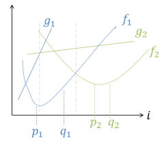
  (a) Before inserting $f_{3}$

  

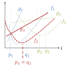
  (b) After inserting $f_{3}$ (value of $p_{1}$ is changed)

  Figure 3: Inserting a new function

  We note one technical detail here: It is possible that $p_{i}$ is already deleted from $L$. This implies that there is another function $f_{i_{j^{\prime}}}$ such that $f_{i_{j^{\prime}}}(p_{i})=f_{i}(p_{i})$ (since we assume that if $p_{i}$ is already deleted, then $f^{*}_{S}(p_{i})$ will never change even when we add more functions to $S$). There are two cases: $j^{\prime}<j$ or $j^{\prime}>j$. For the former case, we know that $f_{i_{j^{\prime}}}(p_{i}-1)<f_{i}(p_{i}-1)$ since $w_{j^{\prime}}>w_{j}$ and thus we simply do nothing ($p_{i}$ will never be returned by AccessMin). For the latter case, we know that $f_{i_{j^{\prime}}}(p_{i}-1)>f_{i}(p_{i}-1)$ and thus we simply set $p_{i}$ to $p_{i}-1$. We deal with the same case for $q_{i}$ similarly.

• DeleteMin($\mathcal{H}$): We delete the node with minimum value from $B$ (which is the one on the top of the heap). This deleted node corresponds to one of the values $f_{1}(p_{1}),f_{2}(p_{2}),\ldots,f_{1}(q_{1}),f_{2}(q_{2}),\ldots$. Assume that $f_{i}(p_{i})$ (resp. $f_{i}(q_{i})$) is such value. We insert a node with value $f_{i}(p_{i}-1)$ (resp. $f_{i}(q_{i}+1)$).

2.3 Using the data structure for semi-matching problem

For any right vertex $v$, we construct a data structure $H_{v}$ as in Section 2.2 to maintain $f_{uv}$, which comes along with $g_{uv}$, for all neighbors of $v$. These functions satisfy the properties above, as shown in Section 2.1. (We note that once $x$ is deleted, $f_{*v}(x)$ will never change since this corresponds to adding a vertex $v_{x}$ to the shortest path tree with distance $f_{*v}(x)$.)

The last issue is how to find $\gamma_{uv}$, the lowest point of an edge $uv$ quickly. We now show an algorithm that finds $\gamma_{uv}$, for every edge $uv\in E$ in time $O(|V|+|E|)$ in total. This algorithm can be run before we start each iteration of the main algorithm (i.e., above Line 4 of Algorithm 2.1). To derive such algorithm, we need the following observation.

Lemma 2.6.

Consider a vertex $v\in V$. Let $u_{1},u_{2},\ldots,u_{\mathrm{deg}(v)}$ be vertices of $U$ incident to $v$, where $w_{u_{1}v}\geq w_{u_{2}v}\geq\ldots\geq w_{u_{\mathrm{deg}(v)}v}$. Then $\gamma_{u_{1}v}\leq\gamma_{u_{2}v}\leq\ldots\leq\gamma_{u_{\mathrm{deg}(v)}v}$.

Proof.

It suffices to show that if $w_{u_{i}v}\geq w_{u_{i+1}v}$, then $\gamma_{u_{i}v}\leq\gamma_{u_{i+1}v}$. We prove this by contrapositive. By Claim 2.5, we conclude that $\gamma_{u_{i}v}$ is the minimum integer $i\in[\mathrm{deg}(v)]$ such that $p(v^{\gamma_{u_{i}v}+1})-p(v^{\gamma_{u_{i}v}})\leq w_{u_{i}v}$, and for any $j<\gamma_{u_{i}v}$, $p(v^{j+1})-p(v^{j})>w_{u_{i}v}$. Thus, if $\gamma_{u_{i}v}>\gamma_{u_{i+1}v}$, then $w_{u_{i+1}v}\geq p(v^{\gamma_{u_{i+1}v}+1})-p(v^{\gamma_{u_{i+1}v}})>w_{u_{i}v}$. This completes the proof. ∎

Algorithm

The following algorithm finds $\gamma_{uv}$ for all $uv\in E$. First, in the preprocessing step (which is done once before we begin the main algorithm), we order edges incident to $v$ decreasingly by their weights, for every vertex $v\in V$. This process takes $O(\mathrm{deg}(v)\log(\mathrm{deg}(v)))$ time. We only have to compute $\gamma_{uv}$ once, so this process does not affect the overall running time.

Next, for any $v\in V$, suppose that the list is $(u_{1},u_{2},\ldots,u_{\mathrm{deg}(v)})$. Since $w_{u_{1}}\geq w_{u_{2}}\geq\ldots\geq w_{\mathrm{deg}(v)}$, it implies that $\gamma_{u_{1}v}\leq\gamma_{u_{2}v}\leq\ldots\leq\gamma_{u_{\mathrm{deg}(v)}v}$ by Lemma 2.6. So, we first find $\gamma_{u_{1}v}$ and then $\gamma_{u_{2}v}$ and so on. This step takes $O(\mathrm{deg}(v))$ for each $v\in V$ and $O(m)$ in total. Therefore, the running time for computing the minimum point $\gamma_{uv}$’s is $O(m\log n)$.

We have now designed our data structure for handling the special structure of the graph $\hat{G}$. This allows us to implement the EKT algorithm on the graph $\hat{G}$ while the algorithm only has to read the structure of the graph $G$. Thus, we solve the weighted semi-matching problem in $O(nm\log{n})$ time.

3 Unweighted semi-matching

In this section, we present an algorithm that finds the optimal semi-matching in unweighted graph in $O(m\sqrt{n}\log n)$ time.

Overview

Our algorithm consists of the following three steps.

In the first step, we reduce the problem to the min-cost flow problem, using the same reduction from Harvey et al. [20]. (See Figure 4.) The details are provided in Section 3.1. We note that the flow is optimal if and only if there is no cost-reducing path (to be defined later). We start with an arbitrary semi-matching and use this reduction to get a corresponding flow. The goal is to eliminate all the cost-reducing paths.

The second step is a divide-and-conquer algorithm used to eliminate all the cost-reducing paths. We call this algorithm CancelAll (cf. Algorithm 3.1). The main idea here is to divide the graph into two subgraphs so that eliminating cost reducing paths “inside” each subgraph does not introduce any new cost reducing paths going through the other. This dividing step needs to be done carefully. We treat this in Section 3.2.

Finally, in the last component of the algorithm we deal with eliminating cost-reducing paths between two sets of vertices quickly. Naively, one can do this using any unit-capacity max-flow algorithm, but this does not give an improvement on the running time. To get a faster algorithm, we observe that the structure of the graph is similar to a unit network, where every vertex has in-degree or out-degree one. Thus, we get the same performance guarantee as that of Dinitz’s algorithm [7, 8]. Details of this part can be found in Section 3.3.

After presenting the algorithm in the next three sections, we analyze the running time in Section 3.4. We note that this algorithm also works in a more general cost function (discussed in Section 3.5). We also observe that there is an $O(n^{5/2}\log n)$-time algorithm that arises directly from the reduction of the weighted case (discussed in Appendix B). This already gives an improvement over the previous results but our result presented here improves the running time further.

3.1 Reduction to min-cost flow and optimality characterization (revisited)

In this section, we review the characterization of the optimality of the semi-matching in the min-cost flow framework. We use the reduction as given in [20]. Given a bipartite graph $G=(U\cup V,E)$, we construct a directed graph $N$ as follows. Let $\Delta$ denote the maximum degree of the vertices in $V$. First, add a set of vertices, called cost centers, $C=\{c_{1},c_{2},\ldots,c_{\Delta}\}$ and connect each $v\in V$ to $c_{i}$ with edges of capacity 1 and cost $i$, for all $1\leq i\leq\mathrm{deg}(v)$. Second, add $s$ and $t$ as a source and sink vertex. For each vertex in $U$, add an edge from $s$ to it with zero cost and unit capacity. For each cost center $c_{i}$, add an edge to $t$ with zero cost and infinite capacity. Finally, direct each edge $e\in E$ from $U$ to $V$ with capacity 1 and cost 0. Observe that the new graph $N$ has $O(n)$ vertices and $O(m)$ edges, and any semi-matching in $G$ corresponds to a max flow in $N$.

Figure 4: Reduction to the min-cost flow problem. Each edge is labeled with (cost, capacity) constraint. Thick edges either are matching edges or contain the flow.

Observe that the new graph $N$ contains $O(n)$ vertices and $O(m)$ edges. It can be seen that any semi-matching in $G$ corresponds to a max flow in $N$. (See example in Figure 4.) Moreover, Harvey et al. [20] proved that an optimal semi-matching in $G$ corresponds to a min-cost flow in $N$; in other words, the reduction described above is correct. Our algorithm is based on observation that the largest cost is $O(|U|)$. This allows one to use the cost-scaling framework to solve the problem.

Now, we review an optimality characterization of the min-cost flow. We need to define a cost-reducing path first. Let $R_{f}$ denote the residual graph of $N$ with respect to a flow $f$. We call any path $p$ from a cost center $c_{i}$ to $c_{j}$ in $R_{f}$ an admissible path and call $p$ a cost-reducing path if $i>j$. A cost-reducing path is one-to-one corresponding to a negative cost cycle implying the condition for the minimality of $f$. Harvey et al. [20] proved the following.

Lemma 3.1 ([20]).

A flow $f$ is a min-cost flow in $N$ if and only if there is no cost-reducing path in $R_{f}(N)$.

Proof.

Note that $f$ is a min-cost flow if and only if there is no negative cycle in $R_{f}$. To prove the “only if” part, assume that there is an cost-reducing path from $c_{i}$ to $c_{j}$. We consider the shortest one, i.e., no cost center is contained in such path except the first and the last vertices. The edges that affect the cost of this path are only the first and the last ones because only edges incident to cost centers have cost. Cost of the first and the last edge is $-i$ and $j$ respectively. Connecting $c_{i}$ and $c_{j}$ with $t$ yields a cycle of cost $j-i<0$.

For the “if” part, assume that there is a negative-cost cycle in $R_{f}$. Consider the shortest cycle which contains only two cost centers, say $c_{i}$ and $c_{j}$ where $i>j$. This cycle contains an admissible path from $c_{i}$ to $c_{j}$. ∎

Given a max-flow $f$ and a cost-reducing path $P$, one can find a flow $f^{\prime}$ with lower cost by augmenting $f$ along $P$ with a unit flow. This is later called path canceling. We are now ready to explain our algorithm.

3.2 Divide-and-conquer algorithm

Our algorithm takes a bipartite graph $G=(U\cup V,E^{\prime})$ and outputs the optimal semi-matching. It starts by transforming $G$ into a graph $N$ as described in the previous section. Since the source $s$ and the sink $t$ are always clear from the context, the graph $N$ can be seen as a tripartite graph with vertices $U\cup V\cup C$; later on, we denote $N=(U\cup V\cup C,E)$. The algorithm proceeds by finding an arbitrary max-flow $f$ from $s$ to $t$ in $N$ which corresponds to a semi-matching in $G$. This can be done in linear time since the flow is equivalent to any semi-matching in $G$.

To find the min-cost flow in $N$, the algorithm uses a subroutine called CancelAll (cf. Algorithm 3.1) to cancel all cost-reducing paths in $f$. Lemma 3.1 ensures that the final flow is optimal.

Algorithm 3.1 CancelAll$(N=(U\cup V\cup C,E))$

1:  if$|C|=1$ then halt endif

2:  Divide C into $C_{1}$ and $C_{2}$ of roughly equal size.

3:  Cancel($N,C_{2},C_{1}$). {Cancel all cost-reducing paths from $C_{2}$ to $C_{1}$}.

4:  Divide $N$ into $N_{1}$ and $N_{2}$ where $N_{2}$ is “reachable” from $C_{2}$ and $N_{1}$ is the rest.

5:  Recursively solve CancelAll$(N_{1})$ and CancelAll$(N_{2})$.

CancelAll works by dividing $C$ and solves the problem recursively. Given a set of cost centers $C$, the algorithm divides $C$ into roughly equal-size subsets $C_{1}$ and $C_{2}$ such that, for any $c_{i}\in C_{1}$ and $c_{j}\in C_{2}$, $i<j$. This guarantees that there is no cost reducing path from $C_{1}$ to $C_{2}$. Then it cancels all cost reducing paths from $C_{2}$ to $C_{1}$ by calling Cancel algorithm (described in Section 3.3).

It is left to cancel the cost-reducing paths “inside” each of $C_{1}$ and $C_{2}$. This is done by partitioning the vertices of $N$ (except $s$ and $t$) and forming two subgraphs $N_{1}$ and $N_{2}$. Then solve the problem separately on each of them. In more detail, we partition the graph $N$ by letting $N_{2}$ be a subgraph induced by vertices reachable from $C_{2}$ in the residual graph and $N_{1}$ be the subgraph induced by the remaining vertices. (Note that both graphs have $s$ and $t$.) For example, in Figure 4, $v_{1}$ is reachable from $c_{3}$ by the path $c_{3},v_{2},u_{2},v_{1}$ in the residual graph.

Lemma 3.2.

CancelAll$(N)$ (cf. Algorithm 3.1) cancels all cost-reducing paths in $N$.

Proof.

Recall that all cost-reducing paths from $C_{2}$ to $C_{1}$ are canceled in line 3. Let $S$ denote the set of vertices reachable from $C_{2}$.

Claim 3.3.

After line 3, no admissible paths between two cost centers in $C_{1}$ intersect $S$.

Proof.

Assume, for the sake of contradiction, that there exists an admissible path from $x$ to $y$, where $x,y\in C_{1}$, that contains a vertex $s\in S$. Since $s$ is reachable from some vertex $z\in C_{2}$, there must exist an admissible path from some vertex in $z$ to $y$; this leads to a contradiction. ∎

This claim implies that, in our dividing step, all cost-reducing paths between pairs of cost centers in $C_{1}$ remain entirely in $N_{1}$. Furthermore, vertices in any cost reducing path between pairs of cost centers in $C_{2}$ must be reachable from $C_{2}$; thus, they must be inside $S$. Therefore, after the recursive calls, no cost-reducing paths between pairs of cost centers in the same subproblems $C_{i}$ are left. The lemma follows if we can show that in these processes we do not introduce more cost-reducing paths from $C_{2}$ to $C_{1}$. To see this, note that all edges between $N_{1}$ and $N_{2}$ remain untouched in the recursive calls. Moreover, these edges are directed from $N_{1}$ to $N_{2}$, because of the maximality of $S$. Therefore there is no admissible path from $C_{2}$ to $C_{1}$. ∎

3.3 Canceling paths from $C_{2}$ to $C_{1}$

In this section, we describe an algorithm that cancels all admissible paths from $C_{2}$ to $C_{1}$ in $R_{f}$, which can be done by finding a max flow from $C_{2}$ to $C_{1}$. To simplify the presentation, we assume that there is a super-source $s$ and super-sink $t$ connecting to vertices in $C_{2}$ and in $C_{1}$, respectively.

To find a maximum flow, observe that $N$ is unit-capacity and every vertex of $U$ has indegree $1$ in $R_{f}$. By exploiting these properties, we show that Dinitz’s blocking flow algorithm [7] can find a maximum flow in $O(|E|\sqrt{|U|})$ time. The algorithm is done by repeatedly augmenting flows through the shortest augmenting paths (see Appendix C).

Lemma 3.4.

Let $d_{i}$ be the length of the shortest $s-t$ path in the residual graph at the $i^{th}$ iteration. For all $i$, $d_{i+1}>d_{i}$.

The lemma can be used to show that Dinitz’s algorithm terminates after $n$ rounds of the blocking flow step, where $n$ is the number of vertices. Since after the $n$-th round, the distance between the source is more than $n$, which means that there is no augmenting path from $s$ to $t$ in the residual graph. The number of rounds can be improved for certain classes of problems. Even and Tarjan [10] and Karzanov [23] showed that in unit capacity networks, Dinitz’s algorithm terminates after $\min(n^{2/3},m^{1/2})$ rounds, where $m$ is the number of edges. Also, in unit networks, where every vertex has in-degree one or out-degree one, Dinitz’s algorithm terminates in $O(\sqrt{n})$ rounds (see, e.g., Tarjan’s book [46]). Since the graph $N$ we are considering is very similar to unit networks, we are able to show that Dinitz’s algorithm also terminates in $O(\sqrt{n})$ in our case.

For any flow $f$, a residual flow $f^{\prime}$ is a flow in a residual graph $R_{f}$ of $f$. If $f^{\prime}$ is maximum in $R_{f}$, $f+f^{\prime}$ is maximum in the original graph. The following lemma relates the amount of the maximum residual flow with the shortest distance from $s$ to $t$ in our case. The proof is a modification of Theorem 8.8 in [46].

Lemma 3.5.

If the shortest $s-t$ distance in the residual graph is $d>4$, the amount of the maximum residual flow is at most $O(|U|/d)$.

Proof.

A maximum residual flow in a unit capacity network can be decomposed into a set $\mathcal{P}$ of edge-disjoint paths where the number of paths equals the flow value. Each of these paths are of length at least $d$. Clearly, each path contains the source, the sink, and exactly two cost centers. Now consider any path $P\in\mathcal{P}$ of length $l$. It contains $l-3$ vertices from $U\cup V$. Since the original graph is a bipartite graph, at least $\lfloor(l-3)/2\rfloor\geq\lfloor(d-3)/2\rfloor\geq(d-4)/2$ vertices are from $U$. Note that each path in $\mathcal{P}$ contains a disjoint set of vertices in $U$, since a vertex in $U$ has in-degree one. Therefore, we conclude that there are at most $2|U|/(d-4)$ paths in $\mathcal{P}$. The lemma follows since each path has one unit of flow. ∎

From these two lemma, we have the main lemma for this section.

Lemma 3.6.

Cancel terminates in $O(|E|\sqrt{|U|})$ time.

Proof.

Since each iteration can be done in $O(|E|)$ time, it is enough to prove that the algorithm terminates in $O(\sqrt{|U|})$ rounds. The previous lemma implies that the amount of the maximum residual flow after the $O(\sqrt{|U|})$-th rounds is $O(\sqrt{|U|})$ units. The lemma thus follows because after that the algorithm augments at least one unit of flow for each round. ∎

3.4 Running time

The running time of the algorithm is dominated by the running time of CancelAll, which can be analyzed as follows. Let $T(n,n^{\prime},m,k)$ denote the running time of the algorithm when $|U|=n,|V|=n^{\prime},|E|=m,$ and $|C|=k$. For simplicity, assume that $k$ is a power of two. By Lemma 3.6, Cancel runs in $O(|E|\sqrt{|U|})$ time. Therefore,

$$T(n,n^{\prime},m,k)\leq c\cdot m\sqrt{n}+T(n_{1},n^{\prime}_{1},m_{1},k/2)+T(n_{2},n^{\prime}_{2},m_{2},k/2),$$

for some constant $c$, where $n_{i},n^{\prime}_{i},$ and $m_{i}$ denote the number of vertices and edges in $N_{i}$, respectively. Recall that each edge participates in at most one of the subproblems; thus, $m_{1}+m_{2}\leq m$. Observe that the number of cost centers always decreases by a factor of two. Thus, the recurrence is solved to $O(\sqrt{n}m\log{k})$. Since $k=O(|U|)$, the running time is $O(\sqrt{n}m\log{n})$ as claimed. Furthermore, the algorithm can work with a more general cost function with the same running time as shown in the next section.

3.5 Generalizations of an unweighted algorithm

The problem can be viewed in a slightly more general version. In Harvey et al. [20], the cost functions for each vertex $v\in V$ are the same. We relax this condition, allowing a different function for each vertex where each function is convex. More precisely, for each $v\in V$, let $f_{v}:{\mathbb{Z}}_{+}\rightarrow{\mathbb{R}}$ be a convex function, i.e., for any $i$, $f_{v}(i+1)-f_{v}(i)\geq f_{v}(i)-f_{v}(i-1)$. The cost for matching $M$ on a vertex $v$ is $f_{v}(\mathrm{deg}_{M}(v))$. In this convex cost function, the transformation similar to what described in Section 3.1 can still be done. However, the number of different values of $f_{v}$ is now $O(|E|)$. So, the size of the set of cost centers $C$ is now upper bounded by $O(|E|)$ not $O(|U|)$. Therefore, the running time of our algorithm becomes $O(|E|\sqrt{|U|}\log{|C|})=O(|E|\sqrt{|U|}\log{|E|})=O(\sqrt{n}m\log{n})$ (since $|E|\leq n^{2}$) which is the same as before.

4 Extension to balanced edge cover problem

The optimal balanced edge cover problem is defined as follows. The input to this problem is a simple undirected graph $G=(V,E)$. An edge cover $F\subseteq E$ is a set of edges such that every vertex of $G$ is incident to at least one edge in $F$. Define the cost of the edge cover $F$ as $\mathrm{cost}(F)=\sum_{v\in{V}}\mathrm{cost}_{F}(v)$, where $\mathrm{cost}_{F}(v)=\sum_{i=1}^{\mathrm{deg}_{F}(v)}i$. (The cost function is the same as that of the unweighted semi-matching problem.) The goal in the optimal balanced edge cover problem is to find an edge cover $F$ with minimum cost.

Observe that any minimal edge cover – including any optimal balanced edge cover – induces a star forest; i.e., every connected component has at most one vertex of degree greater than one (we call such vertices centers) and the rest have degree exactly one. For any minimal edge cover $F$, we call a set of vertices $C$ an extended set of centers of $F$ if (1) $C$ contains all centers of $F$, and (2) each connected component in the subgraph induced by $F$ contains exactly one vertex in $C$.

To solve the balanced edge cover problem using a semi-matching algorithm, we first make a further observation that if we are given an extended set of centers of an optimal balanced edge cover, then an optimal balanced edge cover can be found by simply solving the unweighted semi-matching problem.

Lemma 4.1.

Let $C$ be an extended set of centers of some optimal balanced edge cover $F$. Let $G^{\prime}=((V\setminus C)\cup C,E^{\prime})$ be a bipartite graph where $E^{\prime}$ is the set of edges between $V\setminus C$ and $C$ in $G$. Then any optimal semi-matching in $G^{\prime}$ (where every vertex in $V\setminus C$ touches exactly one edge of the semi-matching) is an optimal balanced edge cover in $G$.

Proof.

Let $M$ be any optimal semi-matching in $G^{\prime}$. First, observe that $F$ is also a semi-matching in $G^{\prime}$. Thus, the cost of $M$ is at most the cost of $F$. It remains to show that $M$ is an edge cover. In other words, we will prove that every vertex in $C$ is covered by $M$.

Assume for the sake of contradiction that there is a vertex $v\in C$ that is not covered by $M$. We show that there exists a cost-reducing path of $M$ starting from $v$ as follows. (The notion of cost-reducing path is defined in Section 3.) Starting from $v_{0}=v$, let $v_{1}$ be any vertex adjacent to $v_{0}$ in $F$. Such $v_{1}$ clearly exists since $F$ is an edge cover. Let $v_{2}$ be a vertex in $C$ adjacent to $v_{1}$ in $M$. Such $v_{2}$ exists and is unique since $v_{1}$ has degree exactly one in $M$. If $\mathrm{deg}_{M}(v_{2})>1$, then we stop the process. Otherwise, we repeat the process by finding a vertex $v_{3}$ adjacent to $v_{2}$ in $F$ and a vertex $v_{4}$ adjacent to $v_{3}$ in $M$. We repeat this until we find $v_{2k}$, for some $k$, such that $\mathrm{deg}_{M}(v_{2})>1$. This process is illustrated in Figure 5.

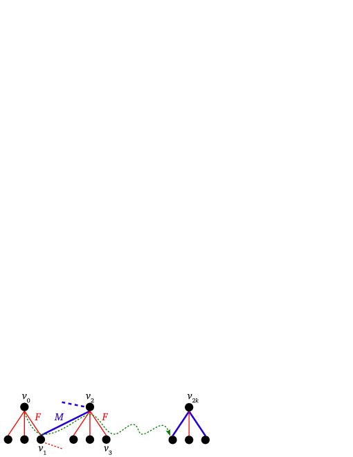
Figure 5: A figure illustrates the construction of a cost-reducing path in Lemma 4.1. Solid thin edges (in red) denote edges in $F$. Solid thick edges (in blue) denote edges in $M$. Dashed thin edges (in red) represent the fact that vertices $v_{i}$, for all odd $i$, have degree exactly one in $F$. Similarly, dashed thick edges (in blue) represent the fact that vertices $v_{i}$, for all even $0<i<2k$, have degree exactly one in $M$ .

Claim 4.2.

All vertices found during the process are distinct.

Proof.

Let $v_{i}$ be the first vertex that appears for the second time, i.e. $v_{i}=v_{j}$ for some $j<i$ and all vertices in $\{v_{0},\ldots,v_{i-1}\}$ are distinct. Let $j<i$ be such that $v_{i}=v_{j}$.

Case 1: $i$ is odd. This means that $v_{i}\notin C$. It follows that $v_{i}$ has degree exactly one in $F$ (this is true for every vertex that is not in the extended set of centers $C$ of $F$). Also note that $(v_{j-1},v_{j})$ and $(v_{i-1},v_{i})$ are both in $F$. Thus, $(v_{j-1},v_{j})=(v_{i-1},v_{i})$. This means that $v_{j-1}=v_{i-1}$, contradicting the assumption that $v_{i}$ is the first vertex that appears for the second time.

Case 2: $i$ is even. This means that $v_{i}\in C$. It follows that $v_{i}$ has degree exactly one in $M$; otherwise, the process must stop when $v_{j}$ is found. As in Case 1, this fact implies that $v_{j-1}=v_{i-1}$ since $(v_{j-1},v_{j})$ and $(v_{i-1},v_{i})$ are both in $M$, contradicting the assumption that $v_{i}$ is the first vertex that appears for the second time. The claim is completed. ∎

The above claim implies that the process will stop. Since we stop at vertex whose degree in $M$ is more than one, the path obtained by this process is a cost-reducing path of $M$. This contradicts the assumption that $M$ is an optimal semi-matching. ∎

It remains to find an extended set of centers. We do this using the following algorithm.

Algorithm Find-Center

First, find a minimum cardinality edge cover $F$. Then find leveling of vertices, denoted by $L_{F}$, as follows.

First, all center vertices of $F$ (i.e., all vertices with degree more than one in $F$) are on level $1$. For $i=1,2,\ldots$, we define level $i+1$ by considering at any vertex $v$ not yet assigned to any level. We pick such vertex $v$ in any order and consider two cases.

• If $i$ is odd and $v$ shares an edge in $F$ with a vertex on level $i$, then we add $v$ to level $i+1$.

• If is $i$ even, then we add $v$ to level $i+1$ if $v$ shares an edge not in $F$ with a vertex on level $i$ and $v$ does not share an edge in $F$ with any vertex on level $i+1$.

We output $C$, the set of even-level vertices, as an extended set of centers. Note that there might be some vertices that are not assigned to any level in $L_{F}$. Figure 6 illustrates the work of the Find-Center algorithm. We first find a minimum edge cover $F$ (consisting of solid edges). Vertices $v_{1}$ and $v_{2}$, which are the centers of the two stars in $F$, are in the first level. The leaves of the stars (i.e., $v_{3},\ldots,v_{8}$) are then in the second level. Vertices $v_{9}$ and $v_{10}$ are both adjacent to vertices in the second level by edges not in $F$. Thus, any of them could be in the third level. However, since they are adjacent in $F$, they could not be both in the third level. If we consider $v_{9}$ before $v_{10}$ in the algorithm, then $v_{9}$ will be in level $3$ while $v_{10}$ will be in level $4$ as in the figure. In this case, $v_{11}$ and $v_{12}$ will not be assigned to any level. In contrast, if we consider $v_{10}$ first, then $v_{9}$, $v_{10}$, $v_{11}$ and $v_{12}$ will be in level $4$, $3$, $5$ and $6$, respectively.

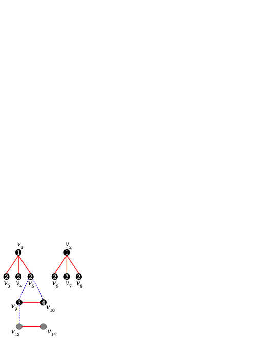
Figure 6: An example of algorithm Find-Center. The solid edges denote edges in the minimum cardinality edge cover $F$, and the dashed edges denote edges not in $F$. The numbers in vertices denote one possible leveling.

Now we analyze the running time and show the correctness of algorithm Find-Center. Once we have these, the main claim of this section follows immediately from Lemma 4.1.

Running time analysis

An edge cover $F$ can be constructed from a maximum cardinality matching by adding one edge incident to each uncovered vertex [14, 35]. The maximum cardinality matching in a bipartite graph can be found by Micali-Vazirani’s algorithm [34] in $O(\sqrt{n}m)$ time or by Harvey’s algorithm [19] in $O(n^{\omega})$ time, where $\omega$ is a time for computing matrix multiplication. Thus, $F$ can be found in $O(\sqrt{n}m)$ time by using the first algorithm. Moreover, finding $L_{F}$ could be done in a breadth-first manner, which takes $O(n+m)$ time. Therefore, the time for the reduction from the balanced edge cover problem to the unweighted semi-matching problem is $O(\sqrt{n}m)$, implying the total running time of $O(\sqrt{n}m\log n)$.

Correctness

We prove the correctness by applying the algorithm BEC1 proposed in [17]. This algorithm starts from any minimum edge cover and keeps augmenting along a cost-reducing path until such path does not exist. Here a cost-reducing path $P$ with respect to an edge cover $F$ is a path starting from any center vertex $u$, following any edge in $F$ and then following an edge not in $F$. The path $P$ keeps using edges in $F$ and edges not in $F$ alternately until it finally uses an edge not in $F$ and ends at a vertex $v$ such that $\mathrm{deg}_{F}(v)\leq\mathrm{deg}_{F}(u)-2$. (See [17] for the formal definition.) It was shown that BEC1 returns an optimal balanced edge cover.

Lemma 4.3.

Let $C$ be a set returned from the algorithm Find-Center. Then $C$ is an extended set of centers of some optimal balanced edge cover $F^{*}$. In other words, there exists an optimal balanced edge cover $F^{*}$ such that all of its centers are in $C$, and each connected component (in the subgraph induced by $F^{*}$) has exactly one vertex in $C$.

Proof.

Let $F$ be a minimum cardinality edge cover found by the algorithm Find-Center. Consider a variant of the algorithm BEC1 where we augment along a shortest cost-reducing path. We will show that we can always augment along the shortest cost-reducing path in such a way that the parity of vertices’ levels never change. To be precise, we construct a sequence of minimum cardinality edge covers $F=F_{1},F_{2},\ldots$ where we obtain $F_{i}$ from $F_{i-1}$ by augmenting along some shortest cost-reducing path. By the following process, we claim that if any vertex is on an odd (even, respectively) level in $L_{F}$, then it is on an odd (even, respectively) level in $L_{F_{i}}$. Moreover, if a vertex belongs to no level in $L_{F}$, then it belongs to no level in $L_{F_{i}}$.

We prove the claim by induction on $i$. The claim trivially holds on $F_{1}=F$. Inductively, assume that the claim holds on some $F_{i}$. Let $P$ be any shortest cost-reducing path with respect to $F_{i}$. If there is no such path $P$, then $F^{*}=F_{i}$ is an optimal edge cover, and we are done. Otherwise, we consider two cases.

• Case 1: The path $P$ contains only vertices on level 1 and 2. This is equivalent to reconnecting vertices on level 2 to vertices on level 1. The level of every vertex is the same in $L_{F_{i}}$ and $L_{F_{i+1}}$. Thus, the claim holds on $F_{i+1}$.

• Case 2: The path $P$ contains a vertex $v_{k}$ not on level 1 or 2. By the construction, $v_{k}$ has degree one in $F$. Thus, $v_{k}$ is the end-vertex of $P$ and all other vertices are on level 1 and 2; otherwise, we can stop at the first vertex that is not on level 1 or 2 and obtain a shorter cost-reducing path. Specifically, we may write $P$ as $P=v_{0}v_{1}\ldots v_{k}$, where vertices $v_{0},v_{1}\ldots,v_{k-1}$ are on level 1 and 2 alternately. Also, $k$ must be even since $P$ is a cost-reducing path. Now, let us augment from $v_{0}$ until we reach $v_{k-2}$. At this point, $v_{k-2}$ must have degree at least three (after the augmentation) because it is on level 1 (which means that it has degree more than one in $F_{i}$) and just got one more edge from the augmentation. If $v_{k}$ is on level 3, then we are done as it will be on level 1 in $L_{F_{i+1}}$, and all vertices in its subtree will be 2 levels higher. Otherwise, $v_{k}$ must be on level 4. Let $a$ be a vertex on level 3 adjacent to $v_{k}$ by an edge in $F_{i}$, which exists by the construction, and let $b$ be a vertex on level 2 adjacent to $a$ by an edge not in $F_{i}$. There are two subcases.

  • Case 2.1: $v_{k-1}=b$. In this case, we augment along the path $v_{1}v_{2}\ldots v_{k-1}a$ instead.

  • Case 2.2: $v_{k-1}\neq b$. In this case, we get an edge cover with cardinality smaller than $|F_{i}|=|F|$ by deleting three edges in $F_{i}$ incident to vertices $b$,$v_{k-1}$,$v_{k}$ and adding edges $(a,b)$ and $(v_{k-1},v_{k})$. (Note that for the case that $b$ is covered by an edge incident to $v_{k-2}$, we use the fact that $v_{k-2}$ has degree at least 3 as discussed earlier.) So, this case is impossible because it contradicts the fact that $F$ is minimum cardinality edge cover.

As there exist augmentations that do not change the parity of vertices’ levels, at the end of the process, we have an optimal balanced edge cover whose extended set of centers is exactly $C$. This completes the proof. ∎

Acknowledgment

We thank David Pritchard for useful suggestions, Jane (Pu) Gao for pointing out some related surveys and Dijun Luo for pointing out some errors in the earlier version of this paper.

APPENDIX

Appendix A Edmonds-Karp-Tomizawa algorithm for weighted bipartite matching

In this section, we briefly explain Edmonds-Karp-Tomizawa (EKT) algorithm. The algorithm starts with an empty matching $M$ and iteratively augments (i.e., increases the size of) $M$. The matching in each iteration is maintained so that it is extreme; i.e., it has the highest weight among matchings of the same cardinality. The augmenting procedure is as follows. Let $M$ be a matching maintained so far. Let $D_{M}$ be the directed graph obtained from $\hat{G}$ by orienting each edge $e$ in $M$ from $\hat{V}$ to $U$ with length $\ell_{e}=-w_{e}$ and orienting each edge $e$ not in $M$ from $U$ to $\hat{V}$ with length $\ell_{e}=w_{e}$. Let $U_{M}$ (respectively, $\hat{V}_{M}$) be the set of vertices in $U$ (respectively, $\hat{V}$) not covered by $M$. If $|M|\neq|U|$, then there is a $U_{M}$-$\hat{V}_{M}$ path. Find a shortest such path, say $P$, and augment $M$ along $P$; i.e., set $M=M\Delta P$. Repeat with the new value of $M$ until $|M|=|U|$.

The bottleneck of this algorithm is the shortest path algorithm. Although $D_{M}$ has negative-length edges, one can find a potential and apply Dijkstra’s algorithm on $D_{M}$ with non-negative reduced cost. The potential and reduced cost are defined as follows.

Definition A.1.

A function $p:U\cup\hat{V}\rightarrow\mathbb{R}$ is a potential if, for every edge $uv$ in the residual graph $D_{M}$, $\tilde{\ell}_{uv}=\ell_{uv}+p(u)-p(v)$ is non-negative. We call $\tilde{\ell}$ a reduced cost with respect to a potential $p$.

The key idea of using a potential is that a shortest path from $u$ to $v$ with respect to a reduced cost $\tilde{\ell}$ is also a shortest path with respect to $\ell$. We omit details here (see, e.g., ([38, Chapter 7 and Section 17.2]), but note that we can use a distance function found in the last iteration of the algorithm as a potential, as in Algorithm 2.1.

Dijkstra’s algorithm.

We now explain Dijkstra’s algorithm on graph $D_{M}$ with non-negative edge weight defined by $\tilde{\ell}$. Our presentation is slightly different from the standard one but will be easy to modify later. The algorithm keeps a subset $X$ of $U\cup\hat{V}$, called set of undiscovered vertices, and a function $d:U\cup\hat{V}\rightarrow\mathbb{R}^{+}$ (the tentative distance). Start with $X=U\cup\hat{V}$ and set $d(u)=0$ for all $u\in U_{M}$ and $d(v)=\infty$ for all $v\notin U_{M}$. Apply the following iteratively:

1:  Find $u\in X$ minimizing $d(u)$ over $u\in X$. Set $X=X\setminus\{u\}$.

2:  For each neighbor $v$ of $u$ in $D_{M}$, relax $uv$, i.e., set $d(v)\leftarrow\min\{d(v),d(u)+\tilde{\ell}_{uv}\}$.

The running time of Dijkstra’s algorithm depends on the implementation. One implementation is by using Fibonacci heap. Each vertex $v\in U\cup\hat{V}$ is kept in the heap with key $d(v)$. Finding and extracting a vertex of minimum tentative distance can be done in an amortized time bound of $O(\log|U\cup\hat{V}|)$ by extract-min operation, and relaxing an edge can be done in an amortized time bound of $O(1)$ by decrease-key operation.

Consider the running time of finding a shortest path. Let $n=|U\cup V|$ and $m=|E|$. We have to call insertion $O(n)$ times, decrease-key $O(m)$ times, and extract-min $O(n)$ times. Thus, the overall running time is $O(m+n\log{n})$.

Appendix B Observation: $O(n^{3})$ and $O(n^{5/2}\log(nW))$ time algorithms

We first recall the reduction from the weighted semi-matching problem to the weighted bipartite matching problem, or equivalently, the assignment problem. Given a bipartite graph $G=(U\cup V,E)$ with edge weight $w$, an instance for the semi-matching problem, we construct a bipartite graph $G=(U\cup\hat{V},\hat{E})$ with weight $\hat{w}$, an instance for the weighted bipartite matching problem, as follows. For every vertex $v\in V$ of degree $deg(v)$, we create exploded vertices $v^{1},v^{2},\ldots,v^{deg(v)}$ in $\hat{V}$ and let $\hat{V}_{v}$ denote a set of such vertices. For each edge $uv$ in $E$ of weight $w_{uv}$, we also create $deg(v)$ edges $uv^{1},uv^{2},\ldots,uv^{deg(v_{i})})$, with associated weights $w_{uv},2\cdot w_{uv},\ldots,\mathrm{deg}(v)\cdot w_{uv}$, respectively. It is easy to verify that finding optimal semi-matching in $G$ is equivalent to finding a minimum matching in $\hat{G}$. Figure 1(a) shows an example of this reduction.

The construction yields a graph $\hat{G}$ with $O(m)$ vertices and $O(nm)$ edges. Thus, applying any existing algorithm for the weighted bipartite matching problem directly is not enough to get an improvement. However, we observe that the reduction can be done in $O(n^{2}\log n)$ time, and we can apply the result of Kao et al. in [22] to reduce the number of participating edges to $O(n^{3})$. Thus, Gabow and Tarjan’s scaling algorithm [12] gives us the following result.

Observation B.1.

If all edges have non-negative integer weight bounded by $W$, then there is an algorithm for the weighted semi-matching problem with the running time of $O(n^{5/2}\log(nW))$.

This result immediately gives an $O(n^{5/2}\log n)$ time algorithm for the unweighted case (i.e., $W=1$). Hence, we already have an improvement upon the previous $O(nm)$ time algorithm for the case of dense graph.

Now, we give an explanation on the observation. If we reduce the problem normally (as in Section 2) to get $\hat{G}$, then the number of edges in $\hat{G}$ and the running time will be $O(nm)$. However, since the size of any matching in the graph $\hat{G}$ is at most $|U|$, it suffices to consider only the smallest $|U|$ edges in $\hat{G}$ incident to each vertex in $U$. Therefore, we may assume that $\hat{G}$ has $O(n^{2})$ edges. (The same observation is also used in [22].)

More precisely, let $E_{u}$ be a set of edges incident to $u$ in $\hat{G}$, and $R$ be a set of $|U|$ smallest edges of $E_{u}$. If the maximum matching of minimum weight, say $M$, contains an edge $e\in E_{u}\setminus R$, then $R\cup\{e\}$ has $|U|+1$ edges. This implies that there is an edge $e^{\prime}\in R$ incident to a vertex $v\in\hat{V}$ not matched by $M$. Thus, we can replace $e$ by $e^{\prime}$ which results in a matching of smaller weight. Therefore, we need to keep only $|U|^{2}$ edges in our reduction. Moreover, we can also reduce the time of the reduction to $O(n^{2}\log{n})$.

The faster reduction is applied at each vertex $u\in U$ as follows. First, we create a binary graph $H$. Each node of $H$ has a key $(e=uv,i)$ and a value $i\cdot w_{e}$, where $e=uv\in E$ and $i$ is an integer. In other words, the value of the node in $H$ with key $(e,i)$ is the weight of an edge $uv^{i}$ in the graph $\hat{G}$. Initially, we add to $H$ a key $(e,1)$ with value $w_{e}$ for all edges $e\in{E}$ incident to $u$. We iteratively extract from $H$ the key $(e=uv,i)$ with minimum value. Then we create an edge $uv^{i}$ in $E^{\prime}$ with weight $i\cdot w_{e}$. If $u$ is incident to less than $|U|$ edges in $E^{\prime}$, then we insert to $H$ a key $(uv,i+1)$ with value $(i+1)\cdot w_{e}$; otherwise, we stop. We repeat the process until the heap $H$ is empty. Thus, the process for each vertex $u\in U$ terminates in $|U|$ rounds. The pseudocode of the reduction is given in Algorithm B.1.

Algorithm B.1 Reduction $(G=(U\cup V,E),w)$

1:  Create an empty set $\hat{E}$, $\hat{V}$.

2:  for all vertices $u\in U$ do

3:     Create a binary heap $H$.

4:     for all edges $e$ incident to $u$ do

5:        Insert to $H$ a node with key $(e,1)$ and value $w(u)$.

6:     end for

7:     for $k\leftarrow 1$ to $|U|$ do

8:        Extract-min from $H$, resulting in $(e=uv,i)$.

9:        Insert to $\hat{V}$ a vertex $v^{i}$ (if it does not exist).

10:        Insert to $\hat{E}$ an edge $uv^{i}$.

11:        Insert to $H$ a node with key $(e=uv,i+1)$ and value $(i+1)\cdot w_{e}$.

12:     end for

13:     Delete the binary heap $H$.

14:  end for

15:  return  $\hat{G}=(U\cup\hat{V},\hat{E})$.

Consider a vertex $u\in U$. At any time during the reduction, there are $O(\mathrm{deg}_{G}(u))$ edges in $H$. So, the extract-min operation takes $O(\log(\mathrm{deg}_{G}(u)))$ time per operation. The time for inserting a vertex to $\hat{V}$ and an edge to $\hat{E}$ is $O(1)$. For each vertex $u\in U$, we have to call insertion $\mathrm{deg}_{G}(u)+|U|$ times and extract-min $|U|$ times. Thus, the time required to process each vertex of $U$ is $O((\mathrm{deg}_{G}(u)+|U|)\log|U|)$. It follows that the total running time of the reduction is $O((|E|+|U|^{2})\log|U|)=O(n^{2}\log n)$.

Now, we run algorithms for the bipartite matching problem on the graph $\hat{G}$ with $n^{2}$ edges. Using Edmonds-Karp-Tomizawa algorithm, the running time becomes $O(nm)=O(n^{3})$. Using Gabow-Tarjan’s scaling algorithm, the running time becomes $O(\sqrt{n}m\log{(nW)}=O(n^{5/2}\log{(nW)})$, where $W$ is the maximum edge weight.

Appendix C Dinitz’s blocking flow algorithm

In this section, we will give an outline of Dinitz’s blocking flow algorithm [7]. Given a network $R$ with source $s$ and sink $t$, a flow $g$ is a blocking flow in $R$ if every path from the source to the sink contains a saturated edge, an edge with zero residual capacity. A blocking flow is usually called a greedy flow since the flow cannot be increased without any rerouting of the previous flow paths. In a unit capacity network, the depth-first search algorithm can be used to find a blocking flow in linear time.

Dinitz’s algorithm works in a layered graph, a subgraph whose edges are in at least one shortest path from $s$ to $t$. This condition implies that we only augment along the shortest paths. The algorithm proceeds by successively find blocking flows in the layered graphs of the residual graph of the previous round. The following is an important property (see, e.g., [2, 38, 46] for proofs). It states that the distance between the source and the sink always increase after each blocking flow step.

In the case of unit-capacity, Even-Tarjan [10] and Karzanov [23] showed algorithm that finds a maximum flow in time $O(\min\{n^{2/3},m^{1/2}\}m)$. In the case of unit-network, i.e., every vertex either has indegree $1$ or outdegree $1$, the algorithm finds a maximum flow in time $O(\sqrt{n}m)$.

References

- [1] D. Abraham. Algorithmics of two-sided matching problems. Master’s thesis, Department of Computer Science, University of Glasgow, 2003.
- [2] Ravindra K. Ahuja, Thomas L. Magnanti, and James B. Orlin. Network flows: theory, algorithms, and applications. Prentice-Hall, Inc., 1993.
- [3] Jacek Blazewicz, Klaus H. Ecker, Erwin Pesch, Günter Schmidt, and Jan Weglarz. Handbook on Scheduling: From Theory to Applications (International Handbooks on Information Systems). Springer, jul 2007.
- [4] Drago Bokal, Bostjan Bresar, and Janja Jerebic. A generalization of hungarian method and Hall’s theorem with applications in wireless sensor networks. Discrete Applied Mathematics, 160(4-5):460–470, 2012.
- [5] John Bruno, E. G. Coffman, Jr., and Ravi Sethi. Algorithms for minimizing mean flow time. In Information processing 74 (Proc. IFIP Congress, Stockholm, 1974), pages 504–510, Amsterdam, 1974. North-Holland.
- [6] John L. Bruno, Edward G. Coffman Jr., and Ravi Sethi. Scheduling independent tasks to reduce mean finishing time. Communications of the ACM, 17(7):382–387, 1974.
- [7] Efim A. Dinic. Algorithm for solution of a problem of maximum flow in networks with power estimation (in russian). Soviet Mathematics Doklady, 11:1277–1280, 1970.
- [8] Yefim Dinitz. Dinitz’ algorithm: The original version and Even’s version. In Essays in Memory of Shimon Even, pages 218–240, 2006.
- [9] Jack Edmonds and Richard M. Karp. Theoretical improvements in algorithmic efficiency for network flow problems. Journal of the ACM, 19(2):248–264, April 1972.
- [10] Shimon Even and Robert Endre Tarjan. Network flow and testing graph connectivity. SIAM Journal on Computing, 4(4):507–518, 1975. Also appeared in STOC 1974.
- [11] Jittat Fakcharoenphol, Bundit Laekhanukit, and Danupon Nanongkai. Faster algorithms for semi-matching problems (extended abstract). In Proceedings of the 37th International Colloquium on Automata, Languages and Programming, pages 176–187, 2010.
- [12] Harold N. Gabow and Robert Endre Tarjan. Faster scaling algorithms for network problems. SIAM Journal on Computing, 18(5):1013–1036, 1989.
- [13] Frantisek Galcík, Ján Katrenic, and Gabriel Semanisin. On computing an optimal semi-matching. In WG, pages 250–261, 2011.
- [14] T. Gallai. Über extreme Punkt- und Kantenmengen. Annales Universitatis Scientiarum Budapestinensis de Rolando Eötvös Nominatae. Sectio Mathematica, 2:133–138, 1959.
- [15] R. L. Graham, E. L. Lawler, J. K. Lenstra, and A. H. G. Rinnooy Kan. Optimization and approximation in deterministic sequencing and scheduling: a survey. Annals of Discrete Mathematics, 5:287–326, 1979. Discrete optimization (Proc. Adv. Res. Inst. Discrete Optimization and Systems Appl., Banff, Alta., 1977), II.
- [16] Yuta Harada, Hirotaka Ono, Kunihiko Sadakane, and Masafumi Yamashita. Optimal balanced semi-matchings for weighted bipartite graphs. IPSJ Digital Courier, 3:693–702, 2007.
- [17] Yuta Harada, Hirotaka Ono, Kunihiko Sadakane, and Masafumi Yamashita. The balanced edge cover problem. In Proceedings of the 19th International Symposium on Algorithms and Computation, pages 246–257, 2008.
- [18] Nicholas J. A. Harvey. Semi-matchings for bipartite graphs and load balancing (slides). http://people.csail.mit.edu/nickh/Publications/SemiMatching/Semi-Matching.ppt, July 2003.
- [19] Nicholas J. A. Harvey. Algebraic algorithms for matching and matroid problems. SIAM Journal on Computing, 39(2):679–702, 2009. Also appeared in FOCS’06.
- [20] Nicholas J. A. Harvey, Richard E. Ladner, László Lovász, and Tami Tamir. Semi-matchings for bipartite graphs and load balancing. Journal of Algorithms, 59(1):53–78, 2006. Conference version in WADS’03.
- [21] W.A. Horn. Minimizing average flow time with parallel machines. Operations Research, pages 846–847, 1973.
- [22] Ming-Yang Kao, Tak Wah Lam, Wing-Kin Sung, and Hing-Fung Ting. An even faster and more unifying algorithm for comparing trees via unbalanced bipartite matchings. Journal of Algorithms, 40(2):212–233, 2001.
- [23] Alexander V. Karzanov. On finding maximum flows in networks with special structure and some applications (in russian). Matematicheskie Voprosy Upravleniya Proizvodstvom, 5:81–94, 1973.
- [24] Anshul Kothari, Subhash Suri, Csaba D. Tóth, and Yunhong Zhou. Congestion games, load balancing, and price of anarchy. In Proceedings of the 1st Workshop on Combinatorial and Algorithmic Aspects of Networking, pages 13–27, 2004.
- [25] Kangbok Lee, Joseph Y.-T. Leung, and Michael L. Pinedo. Scheduling jobs with equal processing times subject to machine eligibility constraints. Journal of Scheduling, 14(1):27–38, 2011.
- [26] Joseph Y.-T. Leung and Chung-Lun Li. Scheduling with processing set restrictions: A survey. International Journal of Production Economics, 116(2):251–262, December 2008.
- [27] Chung-Lun Li. Scheduling unit-length jobs with machine eligibility restrictions. European Journal of Operational Research, 174(2):1325–1328, October 2006.
- [28] Yixun Lin and Wenhua Li. Parallel machine scheduling of machine-dependent jobs with unit-length. European Journal of Operational Research, 156(1):261–266, July 2004.
- [29] Rasaratnam Logendran and Fenny Subur. Unrelated parallel machine scheduling with job splitting. IIE Transactions, 36(4):359–372, 2004.
- [30] László Lovász. The membership problem in jump systems. Journal of Combinatorial Theory, Series B, 70(1):45–66, 1997.
- [31] Chor Ping Low. An efficient retrieval selection algorithm for video servers with random duplicated assignment storage technique. Information Processing Letters, 83(6):315–321, 2002.
- [32] Chor Ping Low. An approximation algorithm for the load-balanced semi-matching problem in weighted bipartite graphs. Information Processing Letters, 100(4):154–161, 2006. Also appeared in TAMC 2006.
- [33] Renita Machado and Sirin Tekinay. A survey of game-theoretic approaches in wireless sensor networks. Computer Networks, 52(16):3047–3061, 2008.
- [34] Silvio Micali and Vijay V. Vazirani. An algorithm for finding maximum matching in general graphs. In Proceedings of the 21st Annual Symposium on Foundations of Computer Science, pages 17–27, 1980.
- [35] Robert Z. Norman and Michael O. Rabin. An algorithm for a minimum cover of a graph. Proceedings of the American Mathematical Society, 10:315–319, 1959.
- [36] Michael Pinedo. Scheduling: Theory, Algorithms, and Systems (2nd Edition). Prentice Hall, August 2001.
- [37] Narayanan Sadagopan, Mitali Singh, and Bhaskar Krishnamachari. Decentralized utility-based sensor network design. Mobile Networks and Applications, 11(3):341–350, 2006.
- [38] Alexander Schrijver. Combinatorial optimization : polyhedra and efficiency. volume A, paths, flows, matchings, chapter 1-38. Springer, 2003.
- [39] René Sitters. Two NP-hardness results for preemptive minsum scheduling of unrelated parallel machines. In Proceedings of the 8th International Conference on Integer Programming and Combinatorial Optimization, pages 396–405, 2001.
- [40] Constantine D. Spyropoulos and David J.A. Evans. Analysis of the Q.A.D. algorithm for an homogeneous multiprocessor computing model with independent memories. International Journal of Computer Mathematics, pages 237–255, 1985.
- [41] Ling-Huey Su. Scheduling on identical parallel machines to minimize total completion time with deadline and machine eligibility constraints. The International Journal of Advanced Manufacturing Technology, 40(5):572–581, 2009.
- [42] Subhash Suri, Csaba D. Tóth, and Yunhong Zhou. Uncoordinated load balancing and congestion games in p2p systems. In Proceedings of the 9th international conference on Peer-to-peer systems, pages 123–130, 2004.
- [43] Subhash Suri, Csaba D. Tóth, and Yunhong Zhou. Selfish load balancing and atomic congestion games. Algorithmica, 47(1):79–96, 2007. Also appeared in SPAA 2004.
- [44] Arie Tamir. Least majorized elements and generalized polymatroids. Mathematics of Operations Research, 20(3):583–589, August 1995.
- [45] Tami Tamir and Benny Vaksendiser. Algorithms for storage allocation based on client preferences. Journal of Combinatorial Optimization, 19(3):304–324, 2010.
- [46] Robert Endre Tarjan. Data structures and network algorithms. Society for Industrial and Applied Mathematics, 1983.
- [47] N. Tomizawa. On some techniques useful for solution of transportation network problems. Networks, 1:173–194, 1971/72.
- [48] Zsuzsanna Vaik. On scheduling problems with parallel multi-purpose machines. Technical Report TR-2005-02, Egerváry Research Group, Budapest, 2005. http://www.cs.elte.hu/egres.