Electronic transport in an anisotropic Sierpinski gasket

Abstract

We present exact results on certain electronic properties of an anisotropic Sierpinski gasket fractal. We use a tight binding Hamiltonian and work within the formalism of a real space renormalization group (RSRG) method. The anisotropy is introduced in the values of the nearest neighbor hopping integrals. An extensive numerical examination of the two terminal transmission spectrum and the flow of the hopping integrals under the RSRG iterations strongly suggest that an anisotropic gasket is more conducting than its isotropic counter part and that, even a minimal anisotropy in the hopping integrals generate continuous bands of eigenstates in the spectrum for finite Sierpinski gaskets of arbitrarily large size. We also discuss the effect of a magnetic field threading the planar gasket on its transport properties and calculate the persistent current in the system. The sensitivity of the persistent current on the anisotropy and on the band filling is also discussed.

I INTRODUCTION

Electronic properties of fractal lattices have been extensively investigated in the past domany -meyer , and a wealth of knowledge has been accumulated. Such deterministic lattices provide excellent examples of systems in between perfect periodic order and complete randomness and exhibit electronic properties drastically different from a crystal and a disordered material. The variable environment around any site of a fractal structure makes such systems quite similar to the random networks. This has motivated a series of experiments to examine the fractal behavior, magneto-resistance and the superconductor-normal phase boundaries on Sierpinski gasket wire networks gordon1 ; gordon2 ; gordon3 ; korshu ; meyer . The interface of theory and experiments has further been strengthened by the recent development of non-dendritic, perfectly self-similar fractal macromolecules of hexagonal Sierpinski gaskets new .

Fractals, in general, exhibit a Cantor set like energy spectrum  domany that is highly degenerate, and the density of states displays a wide variety of singularities. The spectrum may however, broaden up in the presence of a magnetic field banavar . The electronic conductance typically exhibits scaling with a multifractal distribution of the exponents  schwalm2 . One useful tool in investigating regular, finitely ramified fractal lattices has been the real space renormalization group (RSRG) methods. The RSRG approach has been successfully used over the years to unravel, for example, the spectral features of Koch fractals with long range interactions maritan , localization aspects and the length scaling of corner-to-corner propagation in fractal glass and several other interesting fractal networks schwalm1 ; andrade3 .

Interestingly, RSRG studies on fractal lattices reveal another remarkable property of such systems, viz, the existence of an infinite number of isolated extended eigenstates that coexist with an otherwise Cantor set spectrum. This is non trivial, as the fractals as such do not have any long range translational order. Such extended states sometimes are traced back to the existence of multiple cycle fixed points of the Hamiltonian, or have been shown to arise out of a local positional correlation, giving rise to a resonant tunneling effect in some local atomic clusters wang2 ; arun1 ; arun2 ; arun3 . However, no conclusive evidence of the possible formation of a continuum of states has been obtained until very recently, when Schwalm and Moritz schwalm4 have presented exhaustive numerical results to show that a family of fractals does possess a continuum of such states. Incidentally, such continua were also ‘suspected’ in some of the previous studies arun1 ; arun2 ; arun3 , where an external magnetic field was shown to play a role.

This, to our mind, keeps the problem alive, and we look back into the aspect of observing continuous distribution of eigenstates in an anisotropic Sierpinski gasket (SPG) fractal. The magnetic flux, as discussed in the earlier works arun1 ; arun2 ; arun3 through each elementary plaquette of an isotropic SPG breaks the time reversal symmetry of the electron hopping between nearest neighbors. This in turn, already generates a kind of anisotropy in the hopping of an electron when it travels along an angular bond, compared to when it hops along a horizontal bond (Fig. 1). Is anisotropy the factor responsible for any continuum then ? This question is the central motivation behind our present work. Such an issue had been addressed earlier by Hood and Southern hood using a generating function approach coupled with RSRG to come to the conclusion that in an anisotropic SPG only certain hierarchical states persist.

A Second motivation is of course the fact that, grafting a deterministic fractal geometry on a given substrate is quite feasible using the present day advanced nanotechnology and lithographic methods. Therefore, any spectral peculiarity that might come out as a consequence of the anisotropy, and is likely to get reflected in the transport behavior, would be quite possible to observe. This may throw some light into the unaddressed issues related to such deterministic fractal lattices, and will definitely enrich the experimental aspects.

In this communication We examine the transmission spectrum of finite but arbitrarily large anisotropic SPG lattices, with and without any magnetic flux threading the system, using an RSRG decimation method arun1 . In addition to this, we also calculate the persistent current in such a network, and look for any peculiarities in the behavior of the current as well as in the Aharonov-Bohm (AB) oscillations in the transmission that might come out as a result of the anisotropy. To the best of our knowledge, no results are available for persistent currents in an SPG network, specially for the anisotropic case, and the impact of the scale invariant, multiple loop geometry of an SPG on such properties are either very little addressed, or unaddressed at all. Therefore, a thorough study of the problem, together with the literature that already exists will possibly help in obtaining some conclusive result about the spectra of regular fractal lattices under various conditions.

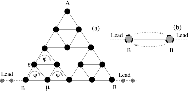
Figure 1: A Sierpinski gasket and its renormalization to a ‘dimer’

We find interesting results. Anisotropy indeed signals the formation of bands of eigenstates with high transmittivity. In general, it is seen that an anisotropic SPG is more conducting compared to its isotropic counterpart. We have carefully carried out an RSRG analysis of the recursion relations of the parameters of the Hamiltonian, and observe certain unusual flow pattern. The transmission coefficient for arbitrarily large lattices has been worked out. In addition to this, we present an in-depth study of the persistent current observed in a SPG network, and the influence of the degree of anisotropy on the current. The behavior of the persistent current is seen to be very sensitive to the degree of anisotropy.

In what follows, we present the results of our investigation. In section II, we present the model and the RSRG method. Section II contains the discussion on the transmission spectrum, while, in section IV we present the results of the calculation of the persistent current.

II THE MODEL AND THE METHOD

We begin by referring to Fig. 1. The Hamiltonian of the network is given by,

$${\mathbf{H}}=\sum_{n}\epsilon_{n}c_{n}^{\dagger}c_{n}+te^{i\theta}\sum_{<nm>}c_{n}^{\dagger}c_{m}+h.c.$$ (1)

where, $c_{n}$ ($c_{n^{\dagger}}$) is the annihilation (creation) operator at the $n$th site of the gasket, the nearest neighbor hopping integral $t=t_{x}$ along the ‘horizontal’ bond and it is equal to $t_{y}$ along any ‘angular’ bond. $\theta=2\pi\phi/\phi_{0}$ is the phase acquired by the electron in hopping along a side of the elementary triangle, as shown in Fig. 1. The phase factor $\theta$ is positive if the electron hops around an elementary triangle in the clockwise sense, and negative otherwise. We have chosen two kinds of ‘on-site’ potentials depending on the local environment of any given site. They are symbolized as $\epsilon$ and $\mu$, and the ‘edge’ sites have potentials $\epsilon_{A}$ and $\epsilon_{B}$ corresponding to the vertices $A$ and $B$. For calculating the end-to-end transmission we have fixed two semi-infinite ordered chains as leads (Fig.1) at the end sites $B$. The on-site potential at the lead-sites has been taken to be constant and equal to $\epsilon_{0}$. The nearest neighbor hopping integral in the leads is chosen as $t_{0}$.

To obtain the transmission coefficient, as well as to judge the nature of the eigenfunctions we renormalize the SPG using a decimation technique arun1 . We first explicitly discuss the anisotropic SPG without any magnetic field. The recursion relations for the on-site potentials and the hopping integrals ( in the absence of any flux threading the gasket) are given by,

$$\epsilon_{n+1} = \epsilon_{n}+\frac{p_{n}+2q_{n}+r_{n}}{\alpha_{n}\beta_{n}-\gamma_{n}}+s_{n}$$

$$\mu_{n+1} = \mu_{n}+u_{n}+v_{n}$$

$$\epsilon_{A,n+1} = \epsilon_{A,n}+\frac{(E-\epsilon_{n})[\beta_{n}t_{y,n}^{2}+\alpha_{n}t_{x,n}^{2}+2t_{x,n}^{2}t_{y,n}^{2}(E-\epsilon_{n}+t_{x,n})]}{\alpha_{n}\beta_{n}-\gamma_{n}}$$

$$\epsilon_{B,n+1} = \epsilon_{B,n}+\frac{\beta_{n}t_{y,n}(E-\epsilon_{n}+t_{x,n})+\gamma_{n}t_{y,n}}{\alpha_{n}\beta_{n}-\gamma_{n}}$$

$$t_{x,n+1} = \frac{[(E-\epsilon_{n})t_{x,n}+t_{y,n}^{2}]^{2}+t_{x,n}t_{y,n}^{2}(E-\mu_{n}+2t_{x,n})-t_{x,n}^{4}}{(E-\epsilon_{n}+t_{x,n})[\beta_{n}-t_{y,n}^{2}-t_{x,n}(E-\mu_{n})]}$$

$$t_{y,n+1} = \frac{t_{y,n}^{2}(E-\mu_{n}+2t_{x,n})}{\beta_{n}-t_{y,n}^{2}-t_{x,n}(E-\mu_{n})}$$ (2)

Here, we have defined,

$$\alpha_{n} = (E-\epsilon_{n})^{2}-t_{x,n}^{2}$$

$$\beta_{n} = (E-\epsilon_{n})(E-\mu_{n})-t_{y,n}^{2}$$

$$\gamma_{n} = t_{y,n}^{2}(E-\epsilon_{n}+t_{x,n})^{2}$$

$$p_{n} = t_{y,n}^{2}\beta_{n}(E-\epsilon_{n})$$

$$q_{n} = t_{x,n}t_{y,n}^{2}(E-\epsilon_{n})(E-\epsilon_{n}+t_{x,n})$$

$$r_{n} = t_{x,n}^{2}\alpha_{n}(E-\epsilon_{n})$$

$$s_{n} = \frac{2t_{y,n}^{2}(E-\epsilon_{n})}{\beta_{n}-t_{y,n}^{2}-t_{x,n}(E-\mu_{n})}$$

$$u_{n} = \frac{2t_{x,n}^{2}(E-\epsilon_{n}+t_{x,n})+t_{y,n}^{2}(E-\mu_{n})}{(E-\mu_{n})(E-\epsilon_{n}+t_{x,n})}$$

$$v_{n} = \frac{t_{y,n}^{2}(E-\mu_{n}+2t_{x,n})^{2}}{(E-\mu_{n})[\beta_{n}-t_{y,n}^{2}-t_{x,n}(E-\mu_{n})]}$$ (3)

Using the above set of equations, we renormalize an $n$-th generation SPG $(n-1)$- times to reduce it to a simple triangle. The top vertex is then decimated to generate an effective diatomic molecule $B-B$ clamped between the leads, as shown in Fig.1(b). The transmission coefficient is then obtained by the standard formula stone ,

$$T=\frac{4\sin^{2}(qa)}{[M_{1,2}-M_{2,1}+(M_{11}-M_{22})\cos(qa)]^{2}+(M_{11}+M_{22})^{2}\sin^{2}(qa)}$$ (4)

where, the matrix elements corresponding to the ‘diatomic molecule’ are given by, $M_{11}=(E-\epsilon_{B,n})^{2}/(t_{0}t_{x,n})-t_{x,n}/t_{0}$, $M_{12}=-M_{21}=-(E-\epsilon_{B,n})/t_{x,n}$, and $M_{22}=-t_{0}/t_{x,n}$. Before ending this section we just point out that the same decimation technique has been used to obtain the recursion relations in the presence of a magnetic field. The recursion relations in the latter case are much more complicated compared to the field-free case, and we decide not to present them here to save space. The role of the magnetic field will however, be discussed in appropriate places. The results are now presented below.

Figure 2: Transmission across a sixth generation isotropic gasket for (a) $\phi=0$, and for (b) $\phi=\phi_{0}/4$. We have chosen $\epsilon_{j}=0$ for all the vertices of the SPG as well as for the sites in the leads, and $t_{x}=t_{y}=t_{0}=1$ throughout.

III RESULTS AND DISCUSSION

III.1 The transmission spectrum and the electron states

The transmission coefficients for the zero-field case and for flux $\phi=\phi_{0}/4$ threading an elementary triangle have been shown in Fig. 2 for a sixth generation SPG in the isotropic limit for the sake of completeness. As is already known arun1 , the magnetic field makes an isotropic gasket more conducting with the signature of continuous zones of transmission. When a slight anisotropy is introduced, and the magnetic field is taken off, it is interesting to observe that, first of all the SPG becomes much more conducting than its isotropic counterpart, and second, once again patches of continuum appear in the transmission spectrum. One such example is presented in Fig. 3 with $t_{x}=0.9$ and $t_{y}=1$. With increasing degree of anisotropy the continua become much more pronounced at places. We have not been able to provide an analytical proof as to whether real continua appear even in such non-translationally invariant systems, but have carried out extensive numerical investigations involving very fine scan of the ‘apparently’ continuous bands found in the transmission spectrum. In every case we find the fine structure in these ‘special’ zones free from any real gaps. Even, the apparently sharp peaks in the transmission spectrum show up finite width when the energy is scanned minutely in their neighborhood. Thus, it is tempting to claim that anisotropy introduces continuous bands of high transmission in fractals such as an SPG. In a recent work Schwalm and Moritz schwalm4 have discussed precisely this issue in the case of a different class of hierarchical lattices. This latest observation gives us confidence in regards of the existence of bands in fractal lattices which can coexist with even a fragmented Cantor like spectrum.

Figure 3: (a) Transmission across a sixth generation anisotropic gasket for $\phi=0$ and with $t_{x}=0.9$ and $t_{y}=1$. (b) Fine scan of the energy interval $[-1.92,-1.8]$ with $\delta E=10^{-}7$. Other parameters are the same as in Fig.2, and energy is measured in unit of the hopping in the leads.

Are these conducting states extended ? To understand this, we have critically examined the flow of the hopping integrals $t_{x}$ and $t_{y}$ under successive RSRG steps. We find two different types of behavior. In general, for an arbitrarily chosen energy both $t_{x}$ and $t_{y}$ flow to zero quickly under iteration. This is understandable, as the spectrum of such a fractal lattice is fragmented in general. So, any arbitrarily chosen energy, in all probability, would either fall in a gap, or would correspond to a localized eigenstate. However, Hood and Southern hood have eliminated the possibility of exponentially localized states in an anisotropic SPG. The flow of the hopping integrals under RSRG changes its pattern when we choose an energy from what apparently looks like a continuum in the transmission spectrum in Fig. 3(a). For any energy within the continuous portion of the spectrum $t_{x}$ remains non-zero for arbitrary number of RSRG loops while the hopping $t_{y}$ ultimately flows to zero. This feature is always true no matter whether the initial value of $t_{x}$ is less or greater than the initial value of $t_{y}$, and persists for any degree of anisotropy. That is, the anisotropy somehow develops a ‘preference’ for $t_{x}$, and breaks the symmetry at all scales of length. Thus, in the infinite lattice limit the entire SPG fractal consists of isolated dimers coupled by the hopping integral $t_{x,n\rightarrow\infty}$. For a finite (but arbitrarily large) SPG we have coupled the semi-infinite leads to the two base atoms ($B-B$). Thus, as $t_{y}$ becomes (practically) zero under RSRG operation, we are left with a perfectly ordered $1$-d chain of atoms with an effective, energy dependent potential connected to its nearest neighbor by a hopping amplitude $t_{x,n\rightarrow\infty}$ (Fig. 4). So, any energy $E$ that will map the original SPG to such a configuration will definitely correspond to a conducting state provided, the energy falls within the allowed band of the leads. What is peculiar about such energy values is that, they apparently form a completely continuous band. We have scanned the spectrum very carefully. One such result of scanning is exhibited in Fig. 3(b), where we have chosen, quite arbitrarily, a certain portion of the spectrum shown in Fig.2a, and scanned the selected zone in an energy interval of $10^{-7}$. It is obvious that the spectrum retains its continuous character.

Before we end this sub-section, it is worth mentioning that, getting a non-zero transmission is definitely connected to the fact that we have attached the leads at the two base atoms of the SPG. Talking about an infinite SPG, we should appreciate that we can build an infinite SPG using a top down approach, when one takes a triangle and keeps on piercing it in the SPG design an infinite number of times. We can keep the leads attached to the base pair of $B$ atoms from the beginning. So, the effective ordered chain of atoms which the SPG boils down to, when we pick up an energy from the continuum, will always be found clamped between the leads. The corresponding state will be extended in the sense that a finite number of sites of the parent SPG will have non-zero amplitudes of the wave function. In the reverse approach, when one builds an infinite SPG by placing SPG’s of previous generations on top of each other, following the growth rule, it is of course not very meaningful to talk about the base atoms such as the $B-B$ pair, or even fixing the leads at the ends. So, at most the infinite system can break up into diatomic clusters as depicted in Fig. 4.

Figure 4: Separation of a finite Sierpinski gasket under RSRG into detached diatomic clusters and linear ordered chain clamped between the leads.

III.2 The Aharonov-Bohm oscillations

The anisotropic SPG displays a wide variety of AB-oscillations which are sensitive to the energy chosen, as well as on the degree of anisotropy. The period of oscillations has been found to be equal to $\phi_{0}/2$ if we choose, say, $E=0$. The AB-oscillations are displayed in Fig. 5 for the cases $(t_{x}=t_{y}=1)$, $(t_{x}=1,t_{y}=2)$ and $(t_{x}=1,t_{y}=10)$. The simple oscillation profile in the isotropic case develops into a profile with multiple peaks and valleys (Fig. 5(b)) as the anisotropy grows larger and finally, in the case of very large degree of anisotropy, the AB-oscillation profile consists of delta-like peaks at special values of the magnetic flux, indicating that, the anisotropic gasket triggers ballistic transmission for $E=0$ only at certain special values of the magnetic flux.

Figure 5: (a) Aharonov-Bohm oscillations in a $4$th generation SPG for $E=0$. (a) Isotropic SPG with $t_{x}=1$ and $t_{y}=1$, (b) anisotropic SPG with $t_{x}=1$, and $t_{y}=2$, and (c) anisotropic SPG with $t_{x}=1$, and $t_{y}=10$. The potential and other parameters are the same as in the previous figures.

III.3 The persistent current

It is well known that a simple Aharonov-Bohm flux threading a metallic or semiconducting ring generates an equilibrium persistent current gefen - jin . With reference to our SPG fractal, where the same flux penetrates each elementary triangular plaquette, the eigenvalues and the eigenstates are flux periodic with period $\phi_{0}$,and hence, as is well known, the equilibrium persistent current carried by the energy level $E_{n}$ is given by,

$$I_{n}=-c\frac{\partial E_{n}}{\partial\phi}$$ (5)

and, the total current in the ring is, $I(\phi)=\sum_{n=1}^{N_{e}}I_{n}$ where, $N_{e}$ is the total number of electrons in the system. It is clear that the nature of the energy spectrum plays a major role in dictating the persistent current in a system. We therefore first have a look at the flux dependence of the eigenvalue spectrum of a $4$-th generation SPG fractal (Fig. 6). For the sake of comparison, we present the spectrum of the SPG in the isotropic limit (Fig. 6, top panel), which shows multiple band crossings, as observed by Rammal and Toulose rammal earlier. The band crossings, related to the symmetry and degeneracy of the eigenvalues at various values of $\phi/\phi_{0}$ are already discussed in details in reference rammal .

Figure 6: Flux dependence of the eigenvalue spectrum of a $4$th generation Sierpinski gasket. (a) The isotropic gasket with $t_{x}=t_{y}=1$, (b) the anisotropic gasket with $t_{x}=1$, $t_{y}=2$, and (c) with $t_{x}=1$ and $t_{y}=10$. In each cast the on-site potential is taken to be zero throughout.

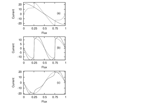
Figure 7: Persistent current in a $4$th generation Sierpinski gasket. (a) The isotropic gasket with $t_{x}=t_{y}=1$. The solid and the dashed curves correspond to $N_{e}=4$ and $15$ respectively. (b) The anisotropic gasket with $t_{x}=1$, $t_{y}=2$ (solid line), and $t_{x}=1$, $t_{y}=10$ (dashed line) with $N_{e}=21$, and (c) Anisotropic gasket with $N_{e}=25$ when $t_{x}=1$, $t_{y}=2$ (solid line) and $t_{x}=1$, $t_{y}=10$ (dashed line). In each cast the on-site potential is taken to be zero throughout.

With the introduction of anisotropy in the hopping integrals ( $t_{x}\neq t_{y}$ ) gaps start to open up in the spectrum lifting the degeneracy in places. As the degree of anisotropy is increased, the spectrum shows clear signature of having groups of states lying close in energy and separated by wider global gaps, that bring a flavor of sub-band structures in the spectrum. The middle and the bottom panels of Fig. 6 represent the anisotropic situation with $t_{x}=1$, $t_{y}=2$ and $t_{x}=1$, $t_{y}=10$ respectively, the last case may be taken as a case of large anisotropy. The flattening of the bands in this case is noteworthy, which finally brings in non trivial changes in the persistent current.

We have examined in details the variation of the persistent current for both the isotropic and anisotropic SPG’s. for the isotropic case with $t_{x}=t_{y}=1$, the current does not exhibit serious deviations (in its qualitative features) from that in a single loop  gefen as long as $N_{e}$ is small. With increasing values of $N_{e}$, a slight rounding off of the $I(\phi)$ is observed. The overall current keeps on increasing as $N_{e}$ increases. The first variation shows up for $N_{e}=10$, when additional kinks appear at $\phi=\phi_{0}/2$. With increasing $N_{e}$ the SPG starts displaying features different from what one finds in simple loop structures. The features persist as we approach the half filled case which, in this study is $N_{e}=21$, when a precise $\phi_{0}/2$ periodicity in $I(\phi)$ is observed. In Fig. 7(a) we show the variation of the persistent current when $N_{e}=4$ (solid line) and $N_{e}=15$ (dashed line).

Introduction of anisotropy in the values of the hopping integral brings in different features in the $I(\phi)$-$\phi$ curves. Though several basic features such as the $\phi_{0}$ periodicity, or the special case of $\phi_{0}/2$ period at $N_{e}=21$ persist, the degree of anisotropy, i.e. the relative values of $t_{x}$ and $t_{y}$ strongly influence the current. Needless to say, the filling factor also plays a crucial role in determining the current profiles. For example, we have found that with $(t_{x},t_{y})=(1,10)$, the current drops compared to the case when $(t_{x},t_{y})=(1,2)$ when we take $N_{e}=21$. This has been tested with several values of the hopping and we come to the conclusion that at half filling, the effect of anisotropy is to reduce the overall current. The current profile becomes smooth with the discontinuous features of isotropic cases for low $N_{e}$ as we introduce anisotropy. This is mainly due to the gaps which open up in the spectrum as the anisotropy is introduced. In this aspect, anisotropy plays a role equivalent to the role that disorder plays in one dimensional rings.

Acknowledgment

The authors are thankful to Santanu K. Maiti for helping out with the graphics, and useful comments on the results of this paper.

References

- (1) E. Domany, S. Alexander, D. Bensimon, and L. P. Kadanoff, Phys. Rev. 28, 3110 (1982).
- (2) R. Rammal and G. Toulose, Phys. Rev. Lett. 49, 1194 (1982).
- (3) J. R. Banavar, L. Kadanoff, and A. M. M. Pruisken, Phys. Rev. B 31, 1388 (1984).
- (4) A. Maritan and A. Stella, Phys. Rev. B 34, 456 (1986).
- (5) J. M. Gordon, A. M. goldman, J. Maps, D. Costello, R. Tiberio, and B. Whitehead, Phys. Rev. Lett. 56, 2280 (1986).
- (6) J. M. Gordon, A. M. Goldman, and B. Whitehead, Phys. Rev. Lett. 59, 2311 (1987).
- (7) J. M. Gordon and A. M. Goldman, Phys. Rev. B 35, 4909 (1987).
- (8) W. A. Schwalm and M. K. Schwalm, Phys. Rev. B 39, 12872 (1989).
- (9) R. F. S. Andrade H. J. Schellnhuber, Europhys. Lett. 10, 73 (1989).
- (10) W. A. Schwalm and M. K. Schwalm, Phys. Rev. B 44, 382 (1991).
- (11) R. F. S. Andrade and H. J Schellnhuber, Phys. Rev. B 44, 13213 (1991).
- (12) W. A. Schwalm and M. K. Schwalm, Phys. Rev. B 47, 7847 (1993).
- (13) P. Kappertz, R. F. S. Andrade, and H. J Schellnhuber, Phys. Rev. B 49, 14711 (1994);
- (14) Z. Lin and M. Goda, Phys. Rev. B 50, 10315 (1994).
- (15) X. R. Wang, Phys. Rev. B 51, 9310 (1994).
- (16) R. F. S. Andrade and H. J Schellnhuber , Phys. Rev. B 55, 12956 (1996).
- (17) Y. Hu, D. C. Tian, and J. Q. You, Phys. Rev. B 53, 5070 (1996).
- (18) R. F. S. Andrade and H. J Schellnhuber, Phys. Rev. B 55, 12956 (1997).
- (19) E. Maciá, Phys. Rev. B 57, 7661 (1998).
- (20) S. E. Korshunov, R. Meyer, and P. Martinoli, Phys. Rev. B 51, 5914 (1995).
- (21) R. Meyer, S. E. Korshunov, Ch. Leemann, and P. Martinoli, Phys. Rev. B 66 104503 (2002).
- (22) G. R. Newkome, P. Wang, C. N. Moorefield, T. J. Cho, P. P. Mohapatra, S. Li, S.-H. wang, O. Lukoyanova, L. Echegoyen, J. A. Palagallo, V. Iancu, and S.-W. Hla, Science 312, 1782 (2006).
- (23) X. R. Wang, Phys. Rev. B 53, 12035 (1996).
- (24) A. Chakrabarti and B. Bhattacharyya, Phys. Rev. B 56, 13768 (1997).
- (25) A. Chakrabarti, Phys. Rev. B 60, 10576 (1999).
- (26) A. Chakrabarti, Phys. Rev. B 72, 134207 (2005)
- (27) W. Schwalm and B. J. Moritz, Phys. Rev. B 71, 134207 (2005).
- (28) M. Hood and B. W. Southern, J. Phys. A: Math. Gen. 19 2679 (1986).
- (29) A. Douglas Stone, J. D. Joannopoulos, and D. J. Chadi, Phys. Rev. B 24, 5583 (1981).
- (30) Ho-Fai Chung, Y. Gefen, E. K. Riedel, and W.-H. Shih, Phys. Rev. B 37, 6050 (1988).
- (31) Ho-Fai Chung, E. K. Riedel, and Y. Gefen, Phys. Rev. Lett. 62, 587 (1989).
- (32) Ho-Fai Chung and E. K. Riedel, Phys. Rev. B 40, 9498 (1989).
- (33) G. J. Jin, Z. D. Wang, A. Hu, and S. S. Jiang, Phys. Rev. B 55, 9302 (1997).
- (34) J. Heinrichs, Int. J. Mod. Phys. 16, 593 (2002).
- (35) Santanu K. Maiti, arXiv, and references therein.