NRG for the bosonic single-impurity Anderson model: Dynamics

Abstract

The bosonic single-impurity Anderson model (B-SIAM) is studied to understand the local dynamics of an atomic quantum dot (AQD) coupled to a Bose-Einstein condensation (BEC) state, which can be implemented to probe the entanglement and the decoherence of a macroscopic condensate. Our recent approach of the numerical renormalization group (NRG) calculation for the B-SIAM revealed a zero-temperature phase diagram, where a $Mott$ phase with local depletion of normal particles is separated from a $BEC$ phase with enhanced density of the condensate. As an extension of the previous work, we present the calculations of the local dynamical quantities of the B-SIAM which reinforce our understanding of the physics in the Mott and the BEC phases.

I Introduction

The observation of the Bose-Einstein condensation (BEC) in ultracold, atomic gases has greatly stimulated research on the properties of this fascinating quantum state of matter. Anglin2002

A particular interest lies in the controlled manipulation of the coherence and the entanglement of the BEC state, Simon2002 ; Heaney2008 ; Heaney2009A ; Heaney2009B which provide the basis of applications such as quantum computing and quantum communications. Nielsen2000 As an example, a new scheme of performing quantum dense coding Bennett1992 and teleportation Bennett1993 was proposed using the spatial-mode entanglement of a single massive boson coupled to a BEC reservoir. Heaney2009A ; Heaney2009B Here one considers a system of two coupled tightly confined potentials, each of which forms one of the spatial modes, $A$ and $B$. In order for the full dense coding protocol to work, $A$ and $B$ have to share a common reference frame with which they can exchange particles. A BEC consisting of an indefinite number of particles fulfills this role Dowling2006 and the coherent control of the BEC state is essential to let a signal between $A$ and $B$ be phase-locked.

On the other hand, there have been extensive studies of decoherence, a process of loosing quantum superpositions due to entanglement between a microscopic system and its environment. Zurek1991 The decoherence mechanism is crucial to understand the transition between quantum and classical systems Leggett1985 ; Leggett2002 in a sense that quantum superposition between distinct states of macroscopic systems is suppressed by the decoherence process. However the environmental effects Zurek1991 ; Leggett1983 make it difficult to probe of the decoherence of macroscopic system directly. As an alternative way, one can use the coupling of a microscopic system, such as an atomic quantum dot, to a mesoscopic or macroscopic system to probe the decoherence of the latter. For instance, there have been several proposals on the single-atom-aided probe of the decoherence of a BEC. Ng2008 ; Bruderer2006 ; Recati2005

In the theoretical schemes above, a BEC state is represented as the Bose-field operator, $\hat{\Psi}_{c}({\bf x})\sim\hat{\rho}({\bf x})^{1/2}e^{-i\hat{\phi}({\bf x})}$ with the density $\hat{\rho}({\bf x})$ and the phase $\hat{\phi}({\bf x})$ of the condensate, of which the only available excitations at low energies are phonons with linear dispersion. However the excitations of a BEC state is phononlike only for wavelengths larger than the healing length $\xi$, where the healing length $\xi$ is defined as the distance over which the condensate wave function grows from zero to the bulk value. In general, the strong collisional interaction in the atomic quantum dot (AQD) can locally break a BEC state to bring up the excitations of normal particles inside of the dot. The bosonic single-impurity Anderson model (B-SIAM) Lee2007 is proposed to describe the normal excitations in the AQD as well as the condensate part.

Another motivation for studing the B-SIAM comes from a treatment of the Bose-Hubbard model within the dynamical mean-field theory (DMFT). Metzner1989 ; Georges1996 The DMFT is an exact theory in infinite spatial dimensions Metzner1989 but, as an approximation for finite dimensional system, it was successful to provide comprehensive understanding about strongly correlated fermion systems. Recently, a new framework of the bosonic DMFT (B-DMFT) was proposed by Byczuk and Vollhardt Byczuk2008 in order to extend the idea of the DMFT to correlated lattice bosons and mixtures of bosons and fermions on a lattice.Byczuk2009 In contrast to the fermionic DMFT (F-DMFT), the lattice model for bosons is mapped into a single-impurity problem with two species of bath spectra, those from the condensate bosons and those from the normal bosons, each of which should be self-consistently determined. The resulting effective bosonic impurity model has been solved by exact diagonalization (ED) method. Hu2009 ; Hubener2009 Results have been presented for various phases at finite temperatures and compared to other theories and the experiments.

The structure of the effective impurity model in the B-DMFT is reduced to the B-SIAM in the absence of the bath spectrum from the condensate bosons, which is the case in the Mott insulating (MI) phase. On the basis of the current work, it will be possible to perform NRG calculations for the B-SIAM with a self-consistently determined bath and investigate transitions between the superfluid (SF) and Mott insulating (MI) phases from the side of MI phase.

The most part in this paper is devoted to discuss the impurity quantum phase transitions of the B-SIAM in terms of the local spectral density. In addition, we present in detail the implementation of the bosonic NRG for the B-SIAM to discuss various strategies to set up the iteration scheme for the bosonic NRG.

The paper is organized as follows: In section II, we introduce the Hamiltonian of the B-SIAM, explaining the differences to the spin-boson model that has been widely used to study the AQD coupled to a superfluid Bose-Einstein condensate. Recati2005 In section III, the formulation of the NRG for the B-SIAM is described in detail. In section IV, we discuss the impurity quantum phase transition of the B-SIAM and explain how the Mott and the BEC phases are discerned in the NRG method. In section V, we turn to the calculation of the local spectral density to discuss the different dynamical properties in Mott and BEC phases. Secion VI is a conclusion. We put some technical details in appendices.

II Model Hamiltonian

The spin-boson model has been widely used for investigating the physical properties of an atomic quantum dot (AQD) coupled to a bosonic reservoir. Heaney2009A ; Heaney2009B ; Ng2008 ; Bruderer2006 ; Recati2005 In Sec. II.1, we summarize the work by Recati et al. Recati2005 , where the particle-exchange between the AQD and the BEC reservoir has been discussed in terms of the spin-boson model. The B-SIAM model is proposed to relax the theoretical constrains in the spin-boson model and describe the density fluctuation of the coherent state originated from the collisional interaction in the AQD. In Sec. II.2, we discuss the basic set-up of the B-SIAM and make a comparision with the spin-boson model.

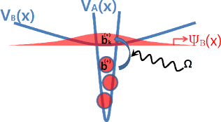
Figure 1: Schematic setup of an atomic quantum dot coupled to a superfluid atomic reservoir. The non-interacting bose particles, denoted by the operator $b_{k}^{(\dagger)}$, are confined in a shallow trap $V_{B}({\bf x})$ and, at zero temperature, condense at the lowest vibrational mode to form a BEC state $\Psi_{B}({\bf x})$ (depicted as a broad wave packet). The creational operator $b^{\dagger}$ add an atom, (depicted by balls) in the tightly confining potential $V_{A}({\bf x})$, where macroscopic condensation is prevented due to the on-site repulsion $U$. The atoms in $V_{B}({\bf x})$ and $V_{A}({\bf x})$ are coupled via a Raman transition with effective Rabi frequency $\Omega$. The confining potential $V_{A}({\bf x})$ and $V_{B}({\bf x})$ are in all three directions with spherical symmetry.

II.1 Atomic quantum dot coupled to a superfluid Bose-Einstein condensate

The particle-exchange mechanism between an AQD and a BEC reservoir was initially proposed by Recati et al. Recati2005 The Hamiltonian is written as

$$H=H_{B}+H_{A}+H_{AB},$$ (1)

where $H_{B}$ and $H_{A}$ correpond the energy of the BEC reservoir and the AQD, respectively. The third term $H_{AB}$ describes the Raman coupling between the AQD and the BEC.

The first term $H_{B}$ describes the dynamics of the BEC reservoir. Here the reservoir atoms are assumed to form a coherent matter wave, held in a shallow trapping potential $V_{B}({\bf x})$ as illustrated in Fig. 1. The wave-function of the coherent state is represented as the Bose-field operator, $\hat{\Psi}_{B}({\bf x})\sim\hat{\rho}({\bf x})^{1/2}e^{-i\hat{\phi}({\bf x})}$, with the density $\hat{\rho}({\bf x})$ and the phase $\hat{\phi}({\bf x})$ of the condensate.

At very low temperature, the coherent matter wave is regarded as superfluid Bose liquid with an equilibrium liquid density $\rho_{B}$, of which the only available excitations are then phonons of low energy $\omega_{\bf q}=v_{s}|{\bf q}|$ with sound velocity $v_{s}$. In this case, the dynamics of the coherent matter wave is described by a hydrodynamic Hamiltonian, Lifshitz1980

$$H_{B}=\frac{1}{2}\int d{\bf x}\left(\frac{\hbar^{2}}{m}\rho_{B}|\nabla{\hat{\phi}}({\bf x})|^{2}+\frac{mv_{s}^{2}}{\rho_{B}}\hat{\Pi}^{2}(x)\right)$$ (2)

where $\rho_{B}$ is the density of the superfluid fraction and $\hat{\Pi}({\bf x})$ is the density fluctuation operator $\hat{\Pi}({\bf x})=\hat{\rho}_{B}({\bf x})-\rho_{B}$, a canonical conjugate of of the superfluid phase $\hat{\phi}({\bf x})$. The quadratic Hamiltonian in Eq. (2) can be written in terms of standard phonon operators $b_{\bf q}$ as

$$H_{B}=\hbar v_{s}\sum_{\bf q}|{\bf q}|b_{\bf q}^{\dagger}b_{\bf q}$$ (3)

via the following transformation, Recati2005

$$\hat{\phi}({\bf x}) = i\sum_{\bf q}|\frac{mv_{s}}{2\hbar{\bf q}V\rho_{B}}|^{1/2}e^{i\bf q\cdot x}(b_{\bf q}-b_{\bf-q}^{\dagger}),$$

$$\hat{\Pi}({\bf x}) = \sum_{\bf q}|\frac{\hbar\rho_{B}\bf q}{2v_{s}Vm}|^{1/2}e^{i\bf q\cdot x}(b_{\bf q}+b_{\bf-q}^{\dagger}).$$ (4)

Here $V$ is the sample volume.

The second term $H_{A}$ corresponds to the on-site energy of the AQD. The AQD is formed by trapping atoms in an additional tightly confining potential $V_{A}({\bf x})$ as shown in Fig. 1. Here one only considers the lowest vibrational mode in the AQD assuming that other higher vibrational modes are off resonant due to large detuning. The collisional interaction of the atoms trapped in the tightly confining potential $V_{A}({\bf x})$ is described by a coupling parameter $g_{AA}=4\pi a_{AA}\hbar^{2}/m$ with scattering lengths $a_{AA}$ and atomic mass $m$. The strength of the collisional interaction between the internal states in the AQD and the coherent state in the BEC reservoir is given as $g_{AB}=4\pi a_{AB}\hbar^{2}/m$. One assumes that atoms in the reservoir are non-interacting. Thus the on-site interaction at the AQD-site is given as,

$$H_{A}=\left[-\hbar\delta+{g_{AB}\int d{\bf x}|\psi_{b}({\bf x})|^{2}\hat{\rho}_{B}({\bf x})}\right]\hat{b}^{\dagger}\hat{b}+\frac{U_{AA}}{2}\hat{b}^{\dagger}\hat{b}^{\dagger}\hat{b}\hat{b},$$ (5)

where $\delta$ is the detuning parameter and $\psi_{A}({\bf x})$ is the wave function of the lowest vibrational mode of the AQD. The on-site repulsion in the AQD is given by the parameter $U_{AA}\sim g_{AA}/l_{A}^{3}$ with $l_{A}$ the size of the ground state wave function $\psi_{A}({\bf x})$.

The last term $H_{AB}$ in Eq. (1) is the laser induced hybridization between particles in the AQD and the BEC reservoir with effective Rabi frequency $\Omega$:

$$H_{AB}=\hbar\Omega\int{d\bf x}(\hat{\Psi}_{B}({\bf x})\hat{\psi}_{A}^{\dagger}({\bf x})+h.c.).$$ (6)

The operator $\hat{\psi}_{A}({\bf x})$ creates an atom in the AQD and the operator $\hat{\Psi}_{B}({\bf x})$ is the annihilation operator for a reservoir atom at the position ${\bf x}$.

The Hamiltonian in Eq. (1) can be reduced to the spin-boson Hamiltonian Leggett1987 under the following conditions. First, one considers the collisional blockade limit of large on-site interaction $U_{AA}$, where only states with occupation $n_{A}=0$ and $1$ in the AQD participate in the dynamics. In this case the internal state of the AQD is described by a pseudospin-1/2, with the spin-up or spin-down state corresponding to occupation by a single or by no atom in the AQD. Using the Pauli matrix notation, the AQD occupation operator $\hat{b}^{\dagger}\hat{b}$ is then replaced by $(1+\sigma_{z})/2$ while $\hat{b}^{\dagger}\rightarrow\sigma_{+}$.

For the BEC state, one assumes that the number of condensate atoms inside the confinement (or the AQD) is much larger than $1$, $n_{B}=\rho_{B}l_{A}^{3}\gg 1$; i.e., the size of the spatial confinement $l_{A}$ is much larger than the average interparticle spacing in the BEC reservoir. Taking the long wave length appriximation, $|{\bf q}|l_{A}\ll 1$, the phonon field operators in $H_{A}$ and $H_{AB}$ are replaced by their values at ${\bf x}=0$. Further, neglecting the density fluctuations in the Raman coupling in Eq. (6), the Hamiltonian $H_{A}$ and $H_{AB}$ can be simplified to

$$H_{A}+H_{AB} = \left(-\frac{\hbar\delta}{2}+\frac{g_{ab}}{2}\hat{\Pi}(0)\right)\sigma_{z}$$ (7)

$$+\frac{\hbar\Delta}{2}\left(\sigma_{+}e^{-i\hat{\phi}(0)}+h.c.\right).$$

Here $\Delta\sim\Omega n_{B}^{1/2}$ is an effective Rabi frequency. Eventually, after a unitary transformation $H=S^{-1}(H_{A}+H_{B}+H_{AB})S$ with $S=\exp\{-\sigma_{z}i\hat{\phi}(0)\}$, the particle-exchange mechanism between a confined boson in AQD and a boson in the BEC reservoir can be described by the spin-boson Hamiltonian,

$$H = -\frac{\hbar\Delta}{2}\sigma_{x}+\sum_{\bf q}\hbar\omega_{\bf q}b_{\bf q}^{\dagger}b_{\bf q}$$ (8)

$$+\left[-\delta+\sum_{\bf q}\lambda_{\bf q}(b_{\bf q}+b_{\bf q}^{\dagger})\right]\frac{\hbar\sigma_{z}}{2}.$$

Here the collisional interactions and those arising from the coupling of the Rabi term to the condensate phase add coherently in the amplitudes of the phonon coupling

$$\lambda_{\bf q}=|\frac{m\hbar{\bf q}v_{s}^{3}}{2V\rho_{B}}|^{1/2}\left(\frac{g_{AB}\rho_{B}}{mv_{s}^{2}}-1\right).$$ (9)

II.2 The bosonic single-impurity Anderson model

The Hamiltonian of the B-SIAM Lee2007 is written as

$$H = \varepsilon{b}^{\dagger}{b}+\frac{U}{2}{b}^{\dagger}{b}({b}^{\dagger}{b}-1)+\sum_{k}\varepsilon_{k}{b}^{\dagger}_{k}{b}_{k}$$ (10)

$$+ \Omega\sum_{k}({b}^{\dagger}{b}_{k}+{b}^{\dagger}_{k}{b}),$$

where ${b}$ and ${b}^{\dagger}$ are annihilation and creation operators obeying bosonic canonical commutation relations and correspond to bosons within a tight trapped potential $V_{A}({\bf x})$, i.e. an AQD. The operators ${b}_{k}$ and ${b}_{k}^{\dagger}$ are annihilation and creation operators corresponding to non-interacting bosons confined in a shallow potential $V_{B}({\bf x})$. Fig. 1 shows the schematic setup.

The energy of the AQD is given by $\varepsilon$ and $U$ is the local repulsion energy when two or more bosons occupy the dot system. The two parameters depend on the strength of the collisional interaction $g_{\alpha\beta}=4\pi a_{\alpha\beta}\hbar^{2}/m$ with scattering length $a_{\alpha\beta}$ ($\alpha,\beta=A$ or $B$) and the Raman detuning $\delta$ as discussed in Sec. II.1.

The third term in Eq. (10) is the kinetic energy of non-interacting bosons confined in the shallow potential $V_{B}({\bf x})$. Here we emphasize that the origin of the bosonic excitations in the B-SIAM is no more restricted to the phonons of the condensate wave function in the lowest vibrational mode in $V_{B}({\bf x})$. Instead, it involves the excited particles to arbitrary higher vibrational modes in the shallow trapping potential $V_{B}({\bf x})$. The number of the vibrational modes in $V_{B}({\bf x})$ becomes infinite as the curvature of the trapping potential approaches to zero. In this case, the shallow trapping potential $V_{B}({\bf x})$ containing free bosons is regarded as an infinite size of a bosonic bath, of which the lowest vibrational mode has zero-energy.

The last term in Eq. (10) is the laser induced hybridization between particles in the AQD and the bosonic bath with effective Rabi frequency $\Omega$. In analogy to the fermionic SIAM the dispersion relation is determined by a hybridization function whose imaginary part, so called bath spectral function, is given by

$$J(\omega) = \pi\Omega^{2}\sum_{k}\delta(\omega-\varepsilon_{k}).$$ (11)

In the following we are interested in systems with gapless bath spectral functions and in low-energy properties. Therefore, we use a model spectral function in the form

$$J(\omega) = \pi\Omega^{2}(1+s)\ \omega_{c}^{-1-s}\omega^{s}\Theta(\omega_{c}-\omega),$$ (12)

where $\Theta(x)$ is a step-like theta function with a cut-off parameter $\omega_{c}$, which yields the total spectral weight $\int_{0}^{\omega_{c}}J(\omega)d\omega=\pi\Omega^{2}$. Note that the choice $\omega_{c}=1$ sets the energy units hereafter. The exponent $s$ characterizes how the bath spectral functions behave in the low-energy regime.

Contrary to the spin-boson model in Ref. (Recati2005, ), the B-SIAM can consider a case where the strong Raman coupling $\Omega$ induces large density fluctuations around the AQD-site. The Raman coupling term in Eq. (10) imposes the spatial displacement to the harmonic oscillators in the bath, which, in consequence, increases the occupation of each vibrational mode. The density of the condensate in the lowest virbational mode increases accordingly. Further, with Rabi coupling $\Omega\sim U$, we go beyond the collisional blockade limit so that an arbitrary number of bosons can occupy the AQD-site to make wide temporal and spatial fluctuation.

It is known that in the strong coupling regime the local spectrum can contain a bound or/and antibound one-particle states in addition to the continuum.logan In this paper we select the coupling strength $\Omega$ such that these extra states do not occur, which is the only restriction for the coupling-strength $\Omega$.

As a final remark we note that the B-SIAM Hamiltonian conserves the total number of bosons. This is in contrast to the spin-boson model,Bulla2003 ; Bulla2005 where the bath contains excited phonons, the number of which is not conserved.

III The Bosonic NRG

III.1 Mapping onto semi-infinite chain

In this section we describe the numerical renormalization group (NRG) method for conserved bosons, which is used to solve the B-SIAM Eq. (10) introduced in the previous section. Details of NRG for bosons are presented in the Appendices. This method is an adoption of the NRG from Ref. (Bulla2005, ) to deal with bosons with a conserved number of particles.

As in the other NRG approaches,Bulla2008 the frequency range $[0,\omega_{c}]$ of the bosonic bath spectral function $J(\omega)$ is divided into intervals $[\omega_{c}\Lambda^{-(n+1)},\omega_{c}\Lambda^{-n}]$, where $\ n=0,1,2,...,$ and $\Lambda>1$ is an NRG discretization parameter. The limit $\Lambda\rightarrow 1$ corresponds to the exact case. Within each of these intervals the spectral function $J(\omega_{c}\Lambda^{-(n+1)}<\omega<\omega_{c}\Lambda^{-n})$ is approximated by its mean value

$$\bar{J}_{n}\equiv\frac{\int_{\omega_{c}\Lambda^{-(n+1)}}^{\omega_{c}\Lambda^{-n}}J(\omega)d\omega}{(\omega_{c}\Lambda^{-n}-\omega_{c}\Lambda^{-(n+1)})}.$$ (13)

Next, following the same steps as in the spin-boson model in Refs. (Bulla2005, ; Lee_PhD, ), we obtain a discretized version of the Hamiltonian (10) with new $V_{n}$ and $\epsilon_{n}$, which are defined on a discrete frequency grid, and with new bath bosonic operators labeled by discrete quantum numbers $n$. Now, this discretized model is mapped onto a semi-infinite chain Bulla2003 ; Bulla2005 ; Bulla2008 and we obtain the following Hamiltonian

$$H = \varepsilon b^{\dagger}b+\frac{U}{2}b^{\dagger}b(b^{\dagger}b-1)+V(b^{\dagger}\bar{b}_{0}+\bar{b}^{\dagger}_{0}b)$$ (14)

$$+ \sum_{m=0}^{\infty}\varepsilon_{m}\bar{b}^{\dagger}_{m}\bar{b}_{m}+\sum_{m=0}^{\infty}t_{m}(\bar{b}^{\dagger}_{m}\bar{b}_{m+1}+\bar{b}^{\dagger}_{m+1}\bar{b}_{m}).$$

The bath degrees of freedom are represented by a tight-binding Hamiltonian with new creation and annihilation operators $\bar{b}_{m}^{(\dagger)}$ and $\bar{b}_{m}$, and the on-site energies $\varepsilon_{m}$, and hopping matrix elements $t_{m}$ between nearest neighbour sites. Both of them fall off exponentially, i.e. $t_{m},\;\varepsilon_{m}\propto\Lambda^{-m}$.Bulla2003 ; Bulla2005 ; Bulla2008 Only the first site of the semi-infinite chain, which is denoted by the index $m=0$, is coupled to the impurity by the hybridization $V$.

The Hamiltonian (14) cannot be diagonalized numerically for the semi-infinite chain. Therefore, we need to truncate it at $m=M-2$, which corresponds to taking $M$ sites, including the impurity-site, in the chain. Since the Hamiltonian parameters $t_{m},\;\varepsilon_{m}$ decay exponentially with $m$, this truncation is justified at large $M$. The Hamiltonian diagonalized numerically has the form

$$H_{M} = \varepsilon b^{\dagger}b+\frac{U}{2}b^{\dagger}b(b^{\dagger}b-1)+V(b^{\dagger}\bar{b}_{0}+\bar{b}^{\dagger}_{0}b)$$

$$+ \sum_{m=0}^{M-2}\varepsilon_{m}\bar{b}^{\dagger}_{m}\bar{b}_{m}+\sum_{m=0}^{M-3}t_{m}(\bar{b}^{\dagger}_{m}\bar{b}_{m+1}+\bar{b}^{\dagger}_{m+1}\bar{b}_{m}).$$

The Hamiltonian (III.1) commutes with the number operator

$$N_{M}=b^{\dagger}b+\sum_{m=0}^{M-2}\bar{b}_{m}^{\dagger}\bar{b}_{m}.$$ (16)

Hence, the eigenstates of $H_{M}$ are also the eigenstates of $N_{M}$, so they are labeled by the corresponding quantum number $N$. The Hilbert space of all states with the same $N$ is denoted by $\mathcal{H}_{N}$. The dimension of each Hilbert space $\mathcal{H}_{N}$ with a given $M$ is

$$\mathcal{D}_{N}=\frac{(M-1+N)!}{(M-1)!\ N!}.$$ (17)

Unfortunately, for large $N$ and $M$ the Hilbert space dimension is so large that direct diagonalization methods are not efficient. Therefore, the Hamiltonian (III.1) is diagonalized iteratively as is discussed next.

III.2 Iterative Diagonalization

At the beginning for small $M$ and $N$ such that the Hilbert space dimension $\mathcal{D}_{N}$ is less than typically few thousands, which depends on the computing facility, we perform exact diagonalization of the Hamiltonian (III.1) for a given M and all possible $N$ such that

$$N=0,1,2,...,N_{\rm max},$$ (18)

where $N_{\rm max}$ is a cutoff for a number of particles. The truncation of the possible particle numbers, which is an approximation, is a necessary to make a computation feasible. As we will see later if the cutoff $N_{\rm max}$ is large enough then it does not affect obtained results.

Having diagonalized the Hamiltonian $H_{M}$ for a given $M$ we increase the system size by adding one more site to the chain. Then we diagonalize the Hamiltonian $H_{M+1}$ which has the form

$$H_{M+1}=H_{M}+\varepsilon_{M-1}\bar{b}^{\dagger}_{M-1}\bar{b}_{M-1}+$$ (19)

$$t_{M-2}(\bar{b}^{\dagger}_{M-2}\bar{b}_{M-1}+\bar{b}^{\dagger}_{M-1}\bar{b}_{M-2}).$$

If it turns out that the dimension of the Hilbert space is too large now, we need to construct an effective representation of the low energy eigenstates while $M$ increases. This is done iteratively as is described below.

We keep the dimension of the Hilbert space constant by taking only the low energy eigenstates. However, to be able to make a direct comparison of the spectra while $M$ increases we need to scale the $M+1$ site Hamiltonian as follows

$$H_{M+1}=\Lambda H_{M}+\Lambda^{M-1}\left[\varepsilon_{M-1}\bar{b}^{\dagger}_{M-1}\bar{b}_{M-1}+\right.$$ (20)

$$\left.t_{M-2}(\bar{b}^{\dagger}_{M-2}\bar{b}_{M-1}+\bar{b}^{\dagger}_{M-1}\bar{b}_{M-2})\right],$$

where we keep the same symbol for the Hamiltonian. All eigenvalues of $H_{M}$ for all $0\leq N\leq N_{\rm max}$ are sorted in an ascending way, and the $N_{s}$ eigenstates $|N,r_{N}\rangle_{M}$ with the lowest eigenvalues are used in diagonalizing $H_{M+1}$. Explicitly, we take into account such states that

$$H_{M}|N,r_{N}\rangle_{M} = E_{r_{N},M}(N)|N,r_{N}\rangle_{M},$$ (21)

with $r_{N}=1,...,n_{s}^{(N)}$, where $n_{s}^{(N)}$ is the number of $N$-particle states with the lowest eigenvalues $E_{r_{N},M}(N)$ in each Hilbert space $\mathcal{H}_{N}$.remark_on_N The dimension of the Hilbert space $N_{s}$ is given by the summation of $n_{s}^{(N)}$,

$$N_{s}=\sum_{N=0}^{N_{max}}n_{s}^{(N)},$$ (22)

and optimized to perform the computation feasible.remark_on_cost

In the Hilbert space of the $H_{M+1}$ Hamiltonian, the $N$-particle states are given by

$$\{|N,R\rangle_{M+1}\}=\{|N-k,r_{N-k}\rangle_{M}\otimes|k\rangle\}_{k=0,...,N},$$ (23)

where

$$|k\rangle=\frac{(\bar{b}_{M-1}^{\dagger})^{k}}{\sqrt{k!}}|0\rangle,$$ (24)

is the $k$-particle state on the $M-1$ site in the chain, and $|0\rangle$ is an empty (vacuum) state on this last site. In Eq. (23) the quantum number $R\equiv r_{N-k}$ means the quantum number of the $H_{M}$ Hamiltonian with $N-k$ particles. The numbers $R$ are not the quantum numbers labeling the eigenstates of the Hamiltonian $H_{M+1}$. This is due to the fact that the new Hamiltonian $H_{M+1}$ does not commute with the total number of particles $N_{M}$ of the previous system with the Hamiltonian $H_{M}$, i.e. we can check that $[H_{M+1},N_{M}]\neq 0$, where $N_{M}$ is defined in (16). In order to find eigenstates of $H_{M+1}$ in a basis (23) we construct the Hamiltonian matrix elements

$$H(R;R^{\prime})\equiv_{M+1}\langle N,R|H_{M+1}|N,R^{\prime}\rangle_{M+1},$$ (25)

and diagonalize this matrix obtaining a set of eigenvalues and eigenstates

$$|N,\omega_{N}\rangle_{M+1}=\sum_{R}U_{N}(\omega_{N};R)|N,R\rangle_{M+1}$$ (26)

where $U_{N}(\omega_{N};R)$ is an orthogonal matrix, and $\omega_{N}$ are new quantum numbers labeling an $N$ particle eigenstate of $H_{M+1}$ with eigenvalue $E_{\omega_{N},M+1}(N)$. The procedure described from Eqs. (23) to (26) is repeated for all $N=0,1,2,...,N_{max}$.

In the next iteration step we extend the system by adding one more site to the chain and use the eigenstates (26) of $H_{M+1}$ to construct a basis of the new Hamiltonian in a way analogous to (23). Repeating the same procedure as described between Eqs. (21) to (26) we obtain new eigenstates and eigenvalues of the larger system. Further details on the iterative diagonalization is presented in Appendix A.

We proceed iterative diagonalizations until the many particle spectra approach the trivial fixed point of the non-interacting bosonic bath. The low-energy spectrum of Mott and BEC phases and the structure of the fixed points are presented in Sec. IV.2.

IV Zero-temperature phase-diagram

IV.1 Overview

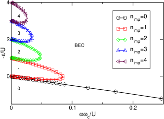
Figure 2: Zero-temperature phase diagram of the B-SIAM for bath exponent $s=0.4$ and fixed impurity Coulomb interaction $U=0.5\omega_{c}$. The different symbols denote the phase boundaries between Mott phases and the BEC phase. The Mott phases are labeled by the number of the impurity-quasiparticle, $n_{imp}$. Only the Mott phases with $n_{imp}\leq 4$ are shown. The NRG parameters are $\Lambda=2.0$, $N_{b}=10$, and $N_{s}=100$.

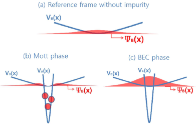
Figure 3: (a) Reference frame: A non-interacting BEC state, $\Psi_{B}({\bf x})$, is confined in a shallow trapping potential $V_{B}({\bf x})$.
(b) Mott phase: The impurity-quasiparticle consists of an integer number of depleted particles, (depicted as balls), which are tightly trapped in $V_{A}({\bf x})$. The other bosons contained in $V_{B}({\bf x})$ still form a BEC cloud but the local density of the condensate vanishes in the vicinity of the AQD. (c) BEC phase: The impurity-quasiparticle forms a part of a BEC state to enhance the density of the condensate around the AQD. The confining potential $V_{A}({\bf x})$ and $V_{B}({\bf x})$ are in all three directions with spherical symmetry.

The zero-temperature phase diagram in Fig. 2 is calculated for fixed $U=0.5\omega_{c}$ with the parameter space spanned by the dimensionless coupling constant $\alpha=\frac{(1+s)}{2}\Omega^{2}$ and the impurity energy $\varepsilon$. We choose $s=0.4$ as the exponent of the power law in $J(\omega)$ in Eq. (12). A similar phase diagram for different bath exponent $s=0.6$ has been presented in Ref. (Lee2007, ). The phase diagram is characterized by a sequence of lobes. We use the terminology “Mott phase” for the inside of the lobes and “BEC phase” for the region outside of the lobes.

The Mott and the BEC phases are distinguished by a hybridized state that is formed around the AQD as illustrated in Fig. 3. Fig. 3-(a) shows a BEC state of a non-interacting bosonic bath, where all existing particles occupy the lowest vibrational mode of the shallow potential $V_{B}({\bf x})$. In the presence of the AQD, however, particles around the AQD can be either completely depleted (Fig. 3-(b)) or even more concentrated toward the local site (Fig. 3-(c)). We call the collective excitation around the AQD as impurity-quasiparticle.

In the Mott phase, the impurity-quasiparticle consist of an integer number of depleted particles, (depicted as balls in Fig. 3-(b)), which are tightly trapped in $V_{A}({\bf x})$. The number of the depleted particles is used to label the different Mott phases in the phase diagram in Fig. 2. The other bosons contained in $V_{B}({\bf x})$ still form a BEC cloud but the local density of the condensate vanishes in the vicinity of the AQD.

In the BEC phase (Fig. 3-(c)), the impurity-quasiparticle forms a part of a BEC state to enhance the density of the condensate around the AQD. The enhancement of the condensate-density is due to the strong Raman coupling $\Omega$ and the deep attractive potential $\varepsilon<0$ of the AQD.

Numerical evidences for our assertions are presented in the rest part of the paper. In Sec. IV.2, we look into the contribution of the impurity-quasiparticle to the ground state energy. In Sec. V, the calculation of the local Greens function is presented to show the local dynamics of normal and condensate particles.

IV.2 Impurity contribution to the ground state energy

The ground state energy of a non-interacting bosonic bath is zero since all existing particles occupy the lowest vibrational mode with zero-energy. An impurity site with repulsive interaction $U$, however, can deplete some particles from the zero-energy mode and shift the ground state energy to be finite. In general, the non-zero ground state energy depends on the total number of particles ($N$) in the system.

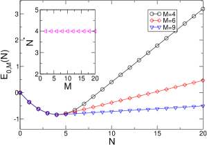
Figure 4: Ground state energy $E_{0,M}(N)$ vs. $N$ calculated for $s=0.6,U=0.1,\varepsilon=-0.36$ and $V=0.01$. The parameters are chosen inside of the Mott lobe labeled by 4 (Mott phase 4). The inset shows the position of the minimum point $N=N^{*}$ as a function of $M$. The NRG parameters used are $\Lambda=1.5$ and $N_{s}=1000$.

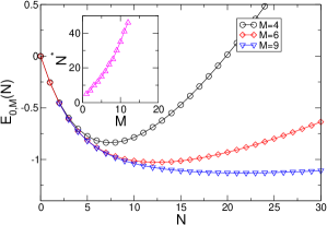
Figure 5: Ground state energy $E_{0,M}(N)$ vs. $N$ calculated for $s=0.6,U=0.1,\varepsilon=-0.05$ and $V=0.4$. The parameters are chosen outside of the Mott lobes (BEC phase). The inset shows the position of the minimum point $N=N^{*}$ as a function of $M$. The NRG parameters used are $\Lambda=1.5$ and $N_{s}=1000$.

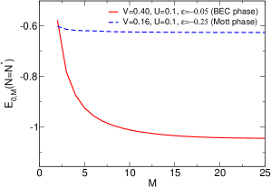
Figure 6: The minimum of the ground state energy $E_{0,M}(N)$ at $N=N^{*}$ as a function of $M$. The solid and dashed lines correspond to the BEC and the Mott phases, respectively. The bath exponent is fixed to $s=0.6$. The NRG parameters used are $\Lambda=1.25$, $N_{max}=40\ (8)$ and $N_{s}=8000\ (600)$ for a BEC (Mott) phase.

Fig. 4 and Fig. 5 show the $N$-dependence of the ground state energy $E_{0,M}(N)$ in Mott and BEC phases, respectively. The different curves are the results from different size ($M$) of the systems. The ground state energy $E_{0,M}(N)$ decreases until the configuration around the AQD, (i.e. impurity-quasiparticle) is optimized. The occupation at the minimum point is denoted by $N^{*}$.

The minimum ground state energy $E_{0,M}(N)$ at $N=N^{*}$ is plotted as a function of the system size $M$ in Fig. 6. The minimum ground state energy $E_{0,M}(N)$ at $N=N^{*}$ converges in the limit $M\rightarrow\infty$. Once the system converges into the large $M$ limit, all ground states for different $N$ become degenerate. Indeed, Fig. 4 and Fig. 5 show that the ground state energy $E_{0,M}(N)$ becomes almost independent of $N$ already for $M=9$.

In the thermodynamic limit ($N\rightarrow\infty$, $M\rightarrow\infty$), the result of adding (or removing) one particle is to convert a state of a system of $N$ particles into the same state of a system of $N\pm 1$ particles:

$$\lim_{N\rightarrow\infty}\lim_{M\rightarrow\infty}|N\pm 1,0\rangle_{M}=\lim_{N\rightarrow\infty}\lim_{M\rightarrow\infty}|N,0\rangle_{M}.$$ (27)

Here $|N,0\rangle_{M}$ is the $N$-particle ground states of $H_{M}$. This is the case of a condensate consisting of a macroscopic number of particles, i.e. a coherent state. Lifshitz1980

The degenerate feature of the ground states in Eq. (27) is extended to the low lying excited states when the many-particle spectrum reaches a fixed point.

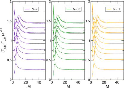
Figure 7: The lowest lying many-particle levels $E_{n,M}\Lambda^{M-1}$ versus iteration number $M$ for parameters $s=0.7$, $V=0.01$, $U=0.5$, and $\varepsilon=-1.2$ (Mott phase). The NRG parameters used are $\Lambda=1.25$, $N_{s}=3000$ and $N_{max}=15$.

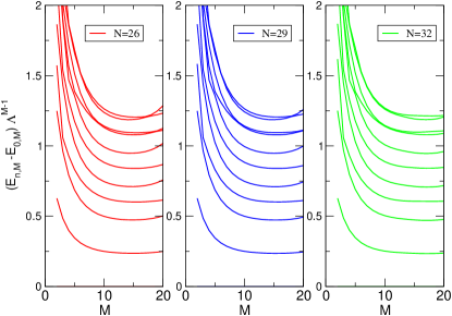
Figure 8: Flow diagram of the lowest lying many-particle levels $E_{n,M}\Lambda^{M-1}$ versus iteration number $M$ for parameters $s=0.7$, $V=0.4$, $U=0.1$ and $\varepsilon=-0.05$. The NRG parameters used are $\Lambda=1.25$, $N_{s}=8000$ and $N_{max}=40$.

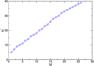
Figure 9: The quasiparticle-occupation $N^{*}$ versus the system-size $M$. The data obtained for parameter parameters $s=0.7$, $V=0.4$, $U=0.1$, and $\varepsilon=-0.05$ (BEC phase). The NRG parameters are $\Lambda=1.25$, $N_{max}=40$ and $N_{s}=8000$.

Fig. 7 shows the energy flow of the lowest lying many-particle levels $E_{n,M}(N)$ versus iteration number $M$. The parameters $V,U$ and $\varepsilon$ are chosen for the system to flow into a Mott phase. Three pannels show the $N$-particle eigenstates for $N=9,10,$ and $11$. The eigenstates in the three figures flow into the same fixed point, which is a trivial fixed point of a non-interacting bosonic bath. It means that the dynamics of the AQD, i.e. the impurity-quasiparticle, is suppressed in this energy-scale so that the low-lying excitations show the dynamics of the non-interacting bosons that locate far from the AQD-site.

Fig. 8 shows the lowest lying many-particle levels in a BEC phase. Three pannels show the $N$-particle eigenstates for $N=26,29,$ and $N=32$, which flow into the same strong-coupling fixed point. The level-spacing in the strong-coupling fixed point is different from the one in the non-interacting fixed point - the reason is not clear yet.

As a last remark, we mention the conditions for numerical convergence. We see that the energy-levels start to deviate from the strong-coupling fixed point around at the iterative step $M=20$. The upturn (deviation from the fixed point) appears if the number of particles $N$ is not large enough compared to $N^{*}(M)$. The $N^{*}$ increases with increasing $M$ (see Fig. 9) and reaches the value $N^{*}\sim 30$ at the iteration $M=20$. The $N$-particle eigenstates flows into the same strong-coupling fixed point only if $N$ is larger than $N^{*}$.

The quick and the slow convergence in Mott and BEC phases respectively can be interpreted as following. The system-size $M$ corresponds to the number of vibrational modes that are taken into account in $H_{M}$, i.e. the larger system involves more vibrational modes with small energy. From this we can conclude that the impurity-quasiparticle in a Mott phase consists of the depleted particles occupying the higher vibrational modes in $V_{B}({\bf x})$, which can be described by a relatively small system size. In a BEC phase, however, the impurity-quasiparticle is a part of a condensate which consists of a macroscopic number of particles with almost zero-energy. Thus one needs a large value of $N$ and $M$ to properly describe the condensate.

V Local dynamics at zero temperature

The local Green’s function of the impurity model is defined as

$$G(z) = \frac{1}{i}\int_{0}^{\infty}dte^{izt}\langle[b(t),b^{\dagger}]\rangle.$$ (28)

where $b^{(\dagger)}$ is an annihilation (creation) operator for the impurity.

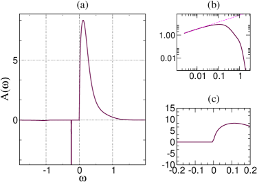
Figure 10: (a) The local spectral density of the B-SIAM for bath exponent $s=0.6$ and fixed impurity Coulomb interaction $U=0.5\omega_{c}$, the onsite impurity energy $\varepsilon=-0.7$, and the hybridization $V=0.15$ (Mott phase 2). The NRG parameters are $\Lambda=1.25$, $N_{max}=3$, and $N_{s}=1000$. (b) The (positive) low-frequency part of $A(\omega)$ (solid line) in log-log scale. The dashed line is a guide line for eyes showing a power-law behavior ($\propto\omega^{s}$, $s=0.6$). (c) The low-frequency part of $A(\omega)$ in linear scale. $A(\omega)$ vanishes at $\omega=0$.

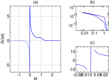
Figure 11: (a) The local spectral density of the B-SIAM for bath exponent $s=0.6$ and fixed impurity Coulomb interaction $U=0.1\omega_{c}$, the onsite impurity energy $\varepsilon=-0.05$, and $V=0.3$ (BEC phase). The NRG parameters are $\Lambda=1.25$, $N_{max}=40$, and $N_{s}=5000$. (b) The low-frequency part of $|A(\omega)|$ as a function of $|\omega|$ in log-log scale, where upper and lower curves correspond to the positive and negative spectral density in the first and third quadrant, respectively. The dashed line in the inset is a guide line for eyes showing a power-law behavior ($\propto\omega^{-s}$, $s=0.6$). (c) The low-frequency part of $A(\omega)$ in linear scale. $A(\omega)$ shows two $\delta$-peaks at $\omega\approx\pm 0.0001$. The position of two peaks approach $\omega=0$ in thermodynamic limit $M\rightarrow\infty$ as seen in Fig. 13.

The local spectral density $A(\omega)$ is the imaginary part of the local Green’s function,

$$A(\omega)=-\frac{1}{\pi}\Im G(\omega+i\delta).$$ (29)

The local spectral density in a Mott phase (Fig. 10) shows two quasiparticle peaks that are separated by a gap, $\Delta_{gap}\sim 0.2$. A sharp peak at $\omega\sim-0.2$ is a signal of hole-excitation in the AQD. The particles trapped in the AQD show no resonance with the reservoir as if they are isolated from it. In fact, most of particles in the reservoir are immobile since they are condensed at zero-energy and make no resonance with the particles in the AQD.

The local occupation at the AQD-site can be obtained by integrating the spectral weight below the chemical potential $\mu=0$,

$$n_{loc}(T=0) = \left[\int_{-\infty}^{\infty}f_{BE}(\omega)A(\omega)d\omega\right]_{T=0}$$ (30)

$$= 1.8875$$

where the Bose-Einstein distribution function $f_{BE}(\omega)$ is given as a step function at zero temperature,

$$\lim_{\beta\rightarrow\infty}f_{BE}(\omega)=\lim_{\beta\rightarrow\infty}\frac{1}{e^{\beta\omega}-1}=-\Theta(-\omega)$$

(31)

with $\Theta(\omega)=1$ for $\omega>0$ and $\Theta(\omega)=0$ for $\omega<0$ .

Creating a particle at the AQD-site gives a broad peak at positive frequency. There is no feature at $\omega=0$ (Fig. 10-(c)) indicating that the BEC is locally forbidden around the AQD-site. The $A(\omega)$ vanishes at $\omega=0$ with a power-law behavior,

$$A(\omega)\propto\omega^{s},\ \omega>0,$$ (32)

which is the same for the bath spectral function $J(\omega)$ in Eq. (12). The power-law behavior for various bath exponents $s$ is shown in Fig. 12-(a).

Fig. 11 shows the spectral density in the BEC phase. The spectral density in the BEC phase (Fig. 11) diverges at $\omega=0$,

$$A(\omega)\propto{\rm sgn}(\omega)|\omega|^{-s},$$ (33)

where the power-law corresponds to the inverse of the bath spectral density $J(\omega)$, see Fig. 11-(b). The divergence of $A(\omega)$ occurs if a hybridized state is pinned at the gapless point of the spectral function $J(\omega)$. To discuss more details, let us look into the local Green’s function $G(z)$ written as

$$G(z)=(z-\varepsilon-\Sigma(z))^{-1}$$ (34)

where $\varepsilon$ is the energy of the impurity level (with operator $b^{(\dagger)}$) and $\Sigma(z)$ is the total self-energy of the impurity model. The imaginary part of the Green’s function in Eq. (34) is given as

$$\Im\left[G(z)\right]=\frac{\Im\left[\Sigma(z)\right]}{(\Re\left[z-\varepsilon-\Sigma(z)\right])^{2}+(\Im\left[\Sigma(z)\right])^{2}}$$ (35)

with $z=\omega+i0^{+}$. The actual calculation of $\Sigma(z)$ is in progress and will be presented in our subsequent paper. Here we assume that the imaginary part of the self-energy $\Im\left[\Sigma(z)\right]$ follows a power-law behavior with the same exponent as the bath spectral function $J(\omega)\propto\omega^{s}$:

$$\Im\left[\Sigma(z)\right]\propto\omega^{s}.$$ (36)

The singular behavior of the local spectral density $A(\omega)$ in Eq. (33) can appear when the impurity bound state occurs at $\omega=0$:

$$\Re\left[\omega-\varepsilon-\Sigma(\omega+i0^{+})\right]=0\ {\rm at\ }\omega=0.$$ (37)

The imaginary part of the self-energy shows a power-law behavior as assumed in Eq. (36). In the case, the $\Im\left[G(z)\right]$ becomes inverse-proportional to $\Im\left[\Sigma(z)\right]$,

$$\Im\left[G(z)\right]\propto\frac{1}{\Im\left[\Sigma(z)\right]}\propto\omega^{-s}.$$ (38)

If the impurity bound state occurs below the chemical potential, the first term in the numerator in Eq. (35) is non-zero at $\omega=0$, which makes $\Im\left[G(z)\right]$ proportional to $\Im\left[\Sigma(z)\right]$ around the gapless point $\omega=0$,

$$\Im\left[G(z)\right]\propto\Im\left[\Sigma(z)\right]\propto\omega^{s}.$$ (39)

A similar feature of $A(\omega)$ is observed in the pseudo-gap Anderson model, remark_on_sgAm ; Bulla2000 where a Kondo bound state appears at the gapless Fermi level.

The singular behavior of $A(\omega)$ for various bath exponents $s$ is shown in Fig. 12-(b).

Another interesting feature in the BEC phase is the finite spectral weight at $\omega=0$ as shown in Fig. 11-(c). Fig. 11-(c) shows two peaks at small frequency $\omega_{0\pm}\approx\pm 0.0001$ with opposite sign of spectral weight. In the limit $M\rightarrow\infty$, the position of both peaks approaches to zero ($\omega=0$) and the amplitude $|\gamma_{0\pm}|$ converges to the same value (Fig. 13). The finite spectral weight at $\omega=0$ indicates the existence of the condensate particles in the AQD-site.

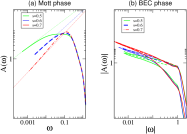
Figure 12: (a) The low-frequency behavior of $A(\omega)$ for $U=0.5\omega_{c}$, $\varepsilon=-0.7$, $V=0.15$ (Mott phase 2) and for various bath-exponent $s=0.5,\ 0.6,$ and $0.7$. (b) The low-frequency behavior of $A(\omega)$ for $U=0.1\omega_{c}$, $\varepsilon=-0.05$, $V=0.3$ (BEC phase) and for various bath-exponent $s=0.5,\ 0.6,$ and $0.7$. The NRG parameters are $\Lambda=1.25$, $N_{max}=40$, and $N_{s}=5000$. The dashed lines are guide lines for eyes to show the power-law behavior. The NRG parameters are $\Lambda=1.25$, $N_{max}=3$, and $N_{s}=1000$.

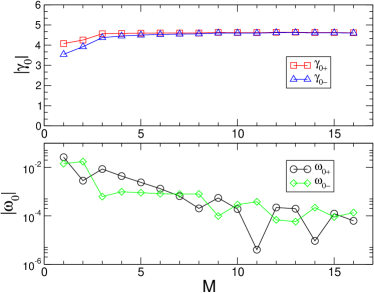
Figure 13: The position ($|\omega_{0\pm}|$) and the amplitude ($|\gamma_{0\pm}|$) of the two peaks in Fig. 11-(c) depending on the size of system $M$. The indices $0+$ ($0-$) denote the peak at positive (negative) frequency, respectively.

The local occupation at the AQD-site can be obtained from integrating the spectral weight below the chemical potential $\mu=0$,

$$n_{loc}(T=0) = \left[\int_{-\infty}^{\infty}f_{BE}(\omega)A(\omega)d\omega\right]_{T=0}$$ (40)

$$= \gamma_{0-}+\lim_{\epsilon\rightarrow 0-}\int_{-\infty}^{\epsilon}A(\omega)d\omega$$

$$= 4.6+0.22$$

where the Bose-Einstein distribution function $f_{BE}(\omega)$ at zero temperature is given in equation (31). The first term ($=4.6$) in equation (40) is the contribution of the condensate particles whereas the second term($=0.22$) is the contribution of particles that are depleted from the condensate.

VI Conclusion

The bosonic single-impurity Anderson model is studied to understand the local dynamics of an atomic quantum dot (AQD) coupled to a BEC state. The major result presented in this paper is the calculation of the impurity Green function but, in addition, considerable space is devoted to refine the description of the Mott and the BEC phases. The local collisional interaction, dominant over the Raman coupling, depletes the particles around the AQD out of the condensate (Mott phase). Otherwise, the Raman transition makes the density of the BEC state even more concentrated toward the local site (BEC phase). The AQD can share a coherent phase of the macroscopic condensate only in the BEC phase and can be used to probe the decoherence of the BEC state. Ng2008 ; Recati2005 ; Bruderer2006

The scheme for the quantum dense coding protocol, Heaney2009A requires two separate AQDs, both of which are coupled to the same BEC state. In Ref. (Heaney2009A, ), it is assumed that a signal between the two AQDs is phase-locked through a BEC state with uniform density and phase. However the phase preserved in each AQD can depend on the position of the dots when the AQDs make the BEC state non-uniform. In this case, the spatial fluctuation of a BEC cloud in the presence of two AQDs deserves of further research, for which a recent extension of the NRG technique, computing spatial correlation function for the Kondo screening cloud, Borda2007 is also applicable.

VII Acknowledgment

We have benefited from discussions with Gun-Sang Jeon, Ki-Seok Kim, Tetsuya Takimoto, Dieter Vollhardt, Xin Wan and Philipp Werner. Special thanks to Vincent Sacksteder for his help on program optimization. This research was supported by the DFG through SFB 484, SFB 608, FOR 960, and TRR 80. H.-J. Lee acknowledges the Max Planck Society and Korea Ministry of Education, Science and Technology for the joint support of the Independent Junior Research Group at the Asia Pacific Center for Theoretical Physics. KB acknowledges the grant N N202 103138 of Polish Ministry of Science and Education.

Appendix A Details about the Iterative Diagonalization

Now we obtain the matrix elements in Eq. (25),

$$H(R;R^{\prime})\equiv_{M+1}\langle N,R|H_{M+1}|N,R^{\prime}\rangle_{M+1},$$ (41)

where the $N$-particle states $|N,R\rangle_{M+1}$ is defined in Eq. (23).

It is straightforward to demonstrate that the diagonal matrix elements of $H_{M+1}$ are

$$H(R;R)=E_{R,M}(N-k)+\ k\ \varepsilon_{M-1}.$$ (42)

The only non-vanishing off-diagonal elements of $H_{M+1}$ are given by

$$H(R^{\prime};R)$$

$$=\delta_{k^{\prime},k-1}t_{M-2}\sqrt{k}\ _{M}\langle N-k^{\prime},R^{\prime}||\bar{b}_{M-2}^{\dagger}||N-k,R\rangle_{M}\$$

$$+\delta_{k^{\prime},k+1}t_{M-2}\sqrt{k+1}\ _{M}\langle N-k^{\prime},R^{\prime}||\bar{b}_{M-2}||N-k,R\rangle_{M},$$

(43)

where $\langle||\bar{b}_{M-2}^{(\dagger)}||\rangle$ are the invariant matrix elements.

In obtaining Eq. (42), we have made use of the following results,

$${}_{M+1}\langle N^{\prime},R^{\prime}||\bar{b}_{M-1}||N,R\rangle_{M+1}=\delta_{k^{\prime},k-1}\sqrt{k}$$ (44)

and

$${}_{M+1}\langle N^{\prime},R^{\prime}||\bar{b}_{M-1}^{\dagger}||N,R\rangle_{M+1}=\delta_{k^{\prime},k+1}\sqrt{k+1}.$$ (45)

which follow from the definition of the basis set in Eq. (23).

From Eq. (42) and Eq. (43), it is clear that we can set up the matrix of $H(R;R^{\prime})$ starting with the knowledge of the previous iterative step such as the eigenenergy $E_{R,M}(N-k)$ and the matrix elements

$${}_{M}\langle N-k-1,r^{\prime}||\bar{b}_{M-2}||N-k,r\rangle_{M}$$ (46)

for $k=0,...,N$.

The actual iteration upon entering the stage $(M+1)$ would proceed as follows. We first start with the lowest allowed value of $N_{M+1}(=0)$, and then increase it in steps of $1$. Within a given $\mathcal{K}_{N}$ subspace, we construct the matrix

$$H(R;R^{\prime})\equiv_{M+1}\langle N,R|H_{M+1}|N,R^{\prime}\rangle_{M+1}.$$ (47)

Diagonalization of this matrix gives a set of eigenstates

$$|N,\omega_{N}\rangle_{M+1}=\sum_{R}U_{N}(\omega_{N};R)|N,R\rangle_{M+1}$$ (48)

where $U_{N}$ will be an orthogonal matrix. The diagonalization means no more than the knowledge of $E_{R,M+1}(N)$ and $U_{N}(\omega_{N};R)$. After completing the diagonalization for one $N$, we proceed up, increasing $N$ in steps of $1$. In order to go to the next iteration we need to calculate ${}_{M+1}\langle N-1,\omega^{\prime}||\bar{b}_{M-1}||N,\omega\rangle_{M+1}$. Using the results in Eq. (44), it is easy to verify that

$${}_{M+1}\langle N-1,\omega_{N-1}^{\prime}||\bar{b}_{M-1}||N,\omega_{N}\rangle_{M+1}$$ (49)

$$= \sum_{R}U_{N-1}(\omega_{N-1}^{\prime};R)U_{N}(\omega_{N};R)\sqrt{k}$$

where $k$ is the number of particles on the $M-1$ site in the chain as given in the Eq. (23).

Appendix B Calculation of local spectral density

The NRG method uses a discretized version of the Anderson model in a semi-infinite chain form in Eq. (III.1). The resulting spectral functions will therefore be given as a set of discrete $\delta$-peaks. For example, the spectral representations of the one-particle Green’s function $G(z)$ is

$$A(\omega) = -\frac{1}{\pi}\Im G(\omega)$$

$$=\sum_{N,r}\sum_{N^{\prime},r^{\prime}}|\langle N,r||b^{\dagger}||N^{\prime},r^{\prime}\rangle|^{2}\exp{\{-\beta E(N,r)\}}$$

$$\ \ \ \ \ \ \ \ \ \ \ \ \ \ \ \times\delta(\omega-E(N,r)+E(N^{\prime},r^{\prime}))$$

$$-\sum_{N,r}\sum_{N^{\prime},r^{\prime}}|\langle N,r||b||N^{\prime},r^{\prime}\rangle|^{2}\exp{\{-\beta E(N,r)\}}$$

$$\ \ \ \ \ \ \ \ \ \ \ \ \ \ \ \times\delta(\omega+E(N,r)-E(N^{\prime},r^{\prime}))$$

Here $|N,r\rangle$ and $E(N,r)$ are the abbreviation of $|N,r\rangle_{M}$ and $E_{M}(N,r)$ in Eq. (21).

As a practical matter, however, calculating the states of $H_{M}$ for large $N$ is hard to deal with because the number of $N$-particle states of $H_{M}$ explodes in combinatorial way as shown in Eq. (17). Thus we introduce cut-off,

$$\sum_{N} \rightarrow \sum_{N=0}^{N_{max}}.$$ (51)

The value of $N_{max}$ has to be larger than the minimum point of the ground state energy at $N=N^{*}$.

At zero temperature, the ensemble average in Eq. (LABEL:gcn-green2) is replaced to the ground expectation value $\langle N^{*},0|...|N^{*},0\rangle$ :

$$A(\omega)_{T=0} = -\frac{1}{\pi}\Im G(\omega)_{T=0}$$

$$= \sum_{r}|\langle N^{*}+1,r|b^{\dagger}|N^{*},0\rangle|^{2}$$

$$\times\delta(\omega-E(N^{*}+1,r)+E(N^{*},0))$$

$$-\sum_{r}|\langle N^{*}-1,r|b|N^{*},0\rangle|^{2}$$

$$\times\delta(\omega+E(N^{*}-1,r)-E(N^{*},0)).$$

The matrix elements $\langle N,r||b^{\dagger}||N^{\prime},r^{\prime}\rangle$ and the energies $E(N,r)$ are calculated in the NRG method. The resulting spectral function, as a set of $\delta$-functions at frequencies $\omega_{n}$ with weights $g_{n}$, are broadened on a logarithmic scale as

$$g_{n}\delta(\omega-\omega_{n})\rightarrow g_{n}\frac{e^{-b_{n}^{2}/4}}{b_{n}\omega_{n}\sqrt{\pi}}\exp[-\frac{(\ln\omega-\ln\omega_{n})^{2}}{b_{n}^{2}}].$$ (53)

In our calculations, the width $b_{n}$ is chosen as b independent of $n$ and the typical values we use are in the range $0.01<b<0.1$. A $\delta$-peak in Fig. 10-(a) is an intrinsic $\delta$-peak without any resonance, for which we use a value, $b_{n}=0.0001$.

References

- (1) R. J. Anglin and W. Ketterle, Nature (London)416, 211 (2002)
- (2) Ch. Simon, Phys. Rev. A 66, 052323 (2002)
- (3) L. Heaney, Ph.D. thesis, University of Leeds, 2008
- (4) L. Heaney and V. Vedral, Phys. Rev. Lett. 103, 200502 (2009)
- (5) L. Heaney and J. Anders, Phys. Rev. A 80, 032104 (2009)
- (6) M. A. Nielsen and I. L. Chuang, Quantum Computation and Quantum information (Cambridge University Press, Cambridge, 2000).
- (7) C. H. Bennett and S. J. Wiesner, Phys. Rev. Lett. 69, 2881 (1992)
- (8) C. H. Bennett et al., Phys. Rev. Lett. 70, 1895 (1993)
- (9) M. R. Dowling, S. D. Bartlet, T. Rudolph, and R. W. Spekkens, Phys. Rev. A 74, 052113 (2006)
- (10) W. H. Zurek, Phys. Today 44, No. 10, 36 (1991)
- (11) A. J. Leggett and A. Garg, Phys. Rev. Lett. 54, 857 (1985)
- (12) A. J. Leggett, J. Phys. Condens. Matter 14, R415 (2002).
- (13) A. O. Cladeira and A. J. Leggett, Physica (Amsterdam) 121A, 587 (1983)
- (14) A. J. Leggett, S. Chakravarty, A. T. Dorsey, M. P. A. Fisher, A. Garg and W. Zwerger, Rev. Mod. Phys. 59, 1 (1987)
- (15) H. T. Ng and S. Bose, Phys. Rev. A 78, 023620 (2008)
- (16) M. Bruderer and D. Jaksch, New J. Phys. 8, 87 (2006)
- (17) A. Recati, P. O. Fedichev, W. Zwerger, J. von Delft and P. Zoller, Phys. Rev. Lett. 94, 040404 (2005)
- (18) H.-J. Lee and R. Bulla, Eur. Phys. J. B 56, 199-203 (2007).
- (19) W. Metzner and D. Vollhardt, Phys. Rev. Lett. 62, 324 (1989)
- (20) A. Georges et al., Rev. Mod. Phys. 68, 13 (1996)
- (21) K. Byczuk and D. Vollhardt, Phys. Rev. B 77, 235106 (2008).
- (22) K. Byczuk and D. Vollhardt, Ann. Phys. (Berlin) 18, 622 (2009).
- (23) W.-J. Hu and N.-H. Tong, Phys. Rev. B 80, 245110 (2009).
- (24) A. Hubener, M. Snoek, and W. Hoffstetter, Phys. Rev. B 80, 245109 (2009).
- (25) E. M. Lifshitz and L. P. Pitaevskii, Statistical Physics, Part II (Pergamon, Oxford, 1980)
- (26) D. Jaksch et al., Phys. Rev. Lett. 82, 1975 (1999)
- (27) R. Bulla, N.-H. Tong and M. Vojta, Phys. Rev. Lett. 91, 170601 (2003).
- (28) R. Bulla, H.-J. Lee, N.-H. Tong and M. Vojta, Phys. Rev. B 71, 045122 (2005).
- (29) R. Bulla, A. C. Hewson and T. Pruschke, J. Phys. Condens. Matter 10, 8365-8380 (1998).
- (30) R. Bulla, Matthew T. Glossop, D. E. Logan and T. Pruschke, J. Phys. Condens. Matter 12, 4899-4921 (2000).
- (31) H. R. Krishna-murthy, J. W. Wilkins, and K. G. Wilson, Phys. Rev. B 21, 1003 (1980).
- (32) D. Withoff and E. Fradkin, Phys. Rev. Lett. 64,1835 (1990).
- (33) M. Vojta, Phil. Mag. 86, 1807 (2006).
- (34) S. Schäfer and D.E. Logan, Phys. Rev. B 63, 45122 (2001); D. Meyer PhD thesis, (Humboldt-Univ. Berlin 2001, unpublished).
- (35) R. Bulla, Th. Costi, and T. Pruschke, Rev. Mod. Phys. 80, 395 (2008).
- (36) H.-J. Lee, PhD thesis, Universty of Augsburg 2007, (unpublished).
- (37) L. Borda, Phys. Rev. B 75, 041307(R) (2007).
- (38) The set of the quantum numbers is different for different . However, they are usualy represented by integers which formally should have a subscript . To avoid this cumbersome notation we add explicitly in the eigenvalues and later for particular cases we use simple integers for .
- (39) The numerical cost depends on , and the total number of iterations . A single job, running in the intel ZEON processor E5430, for parameters , and takes about nine days to complete the process.
-
(40)
In the pseudo-gap Anderson model Withoff1990 , the density of state of a host metal
is assumed to follow power-law behavior,
Here is a band-width of the host metal and is a step-like theta function. In the strong-coupling phase (particle-hole symmetric case), a Kondo bound states pinned at the Fermi level , where becomes gapless. The local spectral density diverges at and the low-frequency behavior is given as Bulla2000(54) (55)