The Integrated Sachs-Wolfe Effect in Time Varying Vacuum Model

Abstract

The integrated Sachs-Wolfe (ISW) effect is an important implication for dark energy. In this paper, we have calculated the power spectrum of the ISW effect in the time varying vacuum cosmological model, where the model parameter $\beta=4.407$ is obtained by the observational constraint of the growth rate. It’s found that the source of the ISW effect is not only affected by the different evolutions of the Hubble function $H(a)$ and the dimensionless matter density $\Omega_{m}(a)$, but also by the different growth function $D_{+}(a)$, all of which are changed due to the presence of matter production term in the time varying vacuum model. However, the difference of the ISW effect in $\Lambda(t)\textmd{CDM}$ model and $\Lambda\textmd{CDM}$ model is lessened to a certain extent due to the integration from the time of last scattering to the present. It’s implied that the observations of the galaxies with high redshift are required to distinguish the two models.

I Introduction

Since 1998, the type Ia supernova (SNe Ia) observations ref:Riess98 ; ref:Perlmuter99 have showed that the expansion of our universe is speeding up rather than slowing down. During these years from that time, many additional observational results, including current Cosmic Microwave Background (CMB) anisotropy measurement from Wilkinson Microwave Anisotropy Probe (WMAP) ref:Spergel03 ; ref:Spergel06 , and the data of the Large Scale Structure (LSS) ref:Tegmark1 ; ref:Tegmark2 , also strongly support this suggestion. In order to understand the mechanism of the accelerating expansion of the universe, the common recognition has been received that there exists an exotic energy component with negative pressure, called dark energy (DE), whose density accounts for two-thirds of the total energy density in the universe according to the current observations. It has been the most important thing to make an effort to probe into what the nature of DE is in the modern cosmology. The simplest and naturalest candidate is the cosmological constant ${\Lambda}$ (vacuum energy) ref:LCDM1 ; ref:LCDM2 , with the equation of state (EOS) $w=\frac{P}{\rho}=-1$. However, it’s pity that it confronts with two difficulties: the fine-tuning problem and the cosmic coincidence problem. An alternative offer is the dynamical DE to alleviate the difficulties above, such as quintessence ref:quintessence , phantom ref:phantom , quintom ref:quintom , generalized Chaplygin gas (GCG) model ref:GCG , Holographic DE ref:holo , and so on.

At present, although in the presence of numerous dark energy models, the concordance model still fits best well with the current combined observations ref:WMAP5 . So it’s necessary to review the cosmic constant problems: The fine-tuning problem is the vacuum energy density predicted by quantum field theory (QFC) is $10^{74}GeV^{4}$, which is about $10^{121}$ orders of magnitude larger than the observed value $10^{-47}GeV^{4}$, so there must be so-called ”fine-tuning” while looking for an balance between two numbers which exits so much discrepancy. The cosmic coincidence problem says: Since the energy densities of vacuum energy and dark matter turn on different evolutions during the expansion history of the universe, why are they nearly equal today and why it happens just now? To get this coincidence, it appears that their ratio must be set to a specific, infinitesimal value in the very early universe. Therefore, in nature the second difficulty is also ”fine-tuning” problem. In the final analysis, both of the two difficulties are related to the energy density of vacuum energy. On the basis of this consideration, a phenomenological and natural attempt at alleviating the above problems is allowing vacuum energy $\Lambda$ to vary ref:LCDM2 ; ref:LtCDM . In $\Lambda(t)\textmd{CDM}$ model, we keep unvaried for the EOS of the vacuum energy, equaling to $-1$, and have an time-evolving energy density. Although the weak point in this ideology is the unknown functional form of the $\Lambda(t)$ parameter, we can deal with the $\Lambda(t)$ parameter by different phenomenologically parameterized form, referring to ref:LCDM2 ; ref:LtCDMparam1 . Meanwhile, the underly explanation for $\Lambda(t)$ parameter has also been explored in the framework of QFT using the renormalization group ref:RG .

The ISW effect ref:ISW1 arises from a time-dependent gravitational potential at late time and leads to CMB temperature anisotropies. From the physical picture point of view, the frequency of the photon released by CMB has been redshifted or blueshifted, which is caused by the decaying gravitational potential, while propagating along the line of light-like from the last scattering surface to now. The ISW effect is a significant implication for dark energy. Since the gravitational potential was an constant during matter-dominated. At the late time, the gravitational potential is time-dependent when dark energy begin to dominate in the universe. So, the detection of ISW effect will provide great support and more information for dark energy. Now, the ISW effect is detected by the cross-correlation between CMB and LSS observations ref:LSS1 ; ref:densitycontrast ; ref:LSS3 ; ref:LSS4 ; ref:LSS5 . In this way, we can separate CMB temperature anisotropies caused by ISW effect from the primary temperature anisotropies.

In this paper, we consider the time varying vacuum model, where a parameterized form of $\Lambda(t)$ is used. The densities of dark matter and vacuum energy don’t conserve independently owing to the time varying vacuum term, which plays the role of the interaction between dark matter and dark energy. The matter production term leads to the different evolutions of the Hubble parameter $H(a)$ and the dimensionless matter density $\Omega_{m}(a)$, and the different structure formation, comparing with the concordance model. Meanwhile, there being a relation between these three quantities and the source term of the ISW effect, we explore the impact from the change of these three quantities on ISW effect in the $\Lambda(t)\textmd{CDM}$ model in theory.

The paper is organized as follows. In next section, we briefly review of the cosmological evolution and structure growth in time varying vacuum model. In section III, we focus on the theory and detection of ISW effect and its power spectrum. The last section is the conclusion.

II Review of the cosmological evolution and structure growth in Time Varying Vacuum Model

Considering a spatially flat Friedmann-Robertson-Walker(FRW) cosmological model, which consists of two components: the dark matter and the dynamic DE. With the metric $ds^{2}=-dt^{2}+a^{2}(t)[dr^{2}+r^{2}(d{\theta}^{2}+\sin^{2}{\theta}d{\phi}^{2})]$, the Friedmann equation and energy-momentum conservation equation can be written as

$$H^{2}=\frac{1}{3M_{pl}^{2}}({\rho}_{m}+{\rho}_{\Lambda}),$$ (1)

$$\frac{d(\rho_{m}+\rho_{\Lambda})}{dt}=-3H(\rho_{m}+P_{m}+\rho_{\Lambda}+P_{\Lambda}),$$ (2)

where, $H=\frac{\dot{a}}{a}$ is the Hubble parameter and $M_{pl}\equiv(8{\pi}G)^{-\frac{1}{2}}$ is the reduced Planck mass. ${\rho}$ and $P$ are density and pressure of a general piece of matter, and their subscripts $m$ and $\Lambda$ respectively correspond to dark matter and dark energy.

In the present paper, we consider the time vacuum energy as dynamic dark energy with energy density $\rho_{\Lambda}=\Lambda(t)M_{pl}^{2}$. In order to simplify the formalism, we work in the framework of geometrical units with $8{\pi}G=c\equiv 1$. Thus, we can obtain the vacuum energy density $\rho_{\Lambda}=\Lambda(t)$ and the corresponding equation of state $P_{\Lambda}=-\rho_{\Lambda}=-\Lambda(t)$. Then the equation (2) reads

$$\frac{d\rho_{m}}{dt}+3H\rho_{m}=-\dot{\Lambda}(t),$$ (3)

which shows that the decaying vacuum density $\Lambda(t)$ plays the role of a source of matter production, and the densities of dark matter and vacuum energy don’t conserve independently. Now, we consider a parameterized form using a power series of $\Lambda(t)$ ref:LtCDMparam1 ; ref:LtCDMparam2 , this is :

$$\Lambda(t)=n_{1}H+n_{2}H^{2}.$$ (4)

Combining the equations (1), (3) and (4), we can get the following Hubble function:

$$H(t)=\frac{n_{1}}{\beta}\frac{e^{\frac{n_{1}t}{2}}}{e^{\frac{n_{1}t}{2}}-1},$$ (5)

where we have defined $\beta=3-n_{2}$. Then with the definition of Hubble function $H(t)=\frac{\dot{a}}{a}$, we proceed with the integration, deriving the evolution of the scale factor of the universe $a(t)$:

$$a(t)=a_{1}(e^{\frac{n_{1}t}{2}}-1)^{\frac{2}{\beta}},$$ (6)

where $a_{1}$ is the constant of integration. Considering the two equations above, we obtain after some algebra that the Hubble function evolves with the scale factor of the universe as follows:

$$H(a)=\frac{n_{1}}{\beta}\left[1+\left(\frac{a(t)}{a_{1}}\right)^{-\frac{\beta}{2}}\right],$$ (7)

where, the parameter $n_{1}$ and the integration constant $a_{1}$ can be reexpressed by taking the Hubble constant $H_{0}$ and the current value of dimensionless dark matter density $\Omega_{m}(a=1)=\Omega_{m0}$ into account with the help of equations (1), (4) and (7):

$$n_{1}=\frac{\beta H_{0}}{1+a_{1}^{\frac{\beta}{2}}},~{}~{}~{}~{}~{}~{}~{}a_{1}=\left(\frac{3\Omega_{m0}}{\beta-3\Omega_{m0}}\right)^{\frac{\beta}{2}}.$$ (8)

Then making use of equation (8), we evaluate the dimensionless dark matter density $\Omega_{m}(a)$ and the dimensionless quantity $E(a)$:

$$\Omega_{m}(a)=\frac{\Omega_{m0}a^{\frac{-\beta}{2}}}{E(a)},$$ (9)

$$E(a)=1-\frac{3\Omega_{m0}}{\beta}+\frac{3\Omega_{m0}}{\beta}a^{\frac{-\beta}{2}}.$$ (10)

From equations (9) and (10), it’s obvious that the Hubble parameter $H(a)$ and the matter density $\Omega_{m}(a)$ scale differently, respectively comparing with their evolutions in the concordance model, due to the decaying vacuum density. In addition, we can get the comoving distance $\chi(a)$ from the solution of the Hubble function $H(a)$ according to its definition of the integration :

$$\chi(a)=\int_{a}^{1}\frac{da}{a^{2}H(a)}.$$ (11)

In the following, we consider the structure growth in the framework of time varying vacuum model. The corresponding Newtonian equation governing the time evolution of dark matter perturbation could be generalized by taking a source of matter production into account ref:growth . It can be written as:

$$\ddot{D}_{+}+(2H+\frac{\epsilon}{\rho_{m}})\dot{D}_{+}-\left[\frac{\rho_{m}}{2}-2H\frac{\epsilon}{\rho_{m}}-\dot{\left(\frac{\epsilon}{\rho_{m}}\right)}\right]D_{+}=0,$$ (12)

where we have defined a growth function $D_{+}(a)=\frac{\delta(x,a)}{\delta(x,a=1)}$, an equivalent and convenient quantity describing the growth of dark matter density inhomogeneities. $\epsilon$ is the source of matter production, and here it is given by $\epsilon=-\dot{\Lambda}(t)$. On account of the presence of $\epsilon$, it’s seen that equation (12) is different from the well-known linear matter perturbation equation.

There are two solutions to the differential equation (12), where one is a growing mode and the other is a decaying mode. Since almost all current models of the universe have a non-increasing Hubble rate, we are interested in the growing one, which is given by ref:LtCDMparam1 ; ref:LtCDMparam2 :

$$D_{+}(a)=\frac{9\Omega_{m0}^{2}}{2\beta}\left(\frac{\beta-3\Omega_{m0}}{3\Omega_{m0}}\right)^{\frac{2\beta-4}{\beta}}a^{\frac{\beta-6}{2}}\int_{0}^{a}\frac{dx}{x^{\frac{\beta}{2}}E^{2}(x)}.$$ (13)

Next, we constrain the $\Lambda(t)CDM$ model parameter $\beta$ according to the growth rate of clustering:

$$f(a)=\frac{a}{D_{+}(a)}\frac{dD_{+}(a)}{da}.$$ (14)

redshift z		$f_{obs}$		Reference
$0.15$		$0.51\pm 0.11$		ref:fobs1
$0.35$		$0.70\pm 0.18$		ref:fobs2
$0.55$		$0.75\pm 0.18$		ref:fobs3
$0.77$		$0.91\pm 0.36$		ref:fobs4
$1.4$		$0.90\pm 0.24$		ref:fobs5
$3.0$		$1.46\pm 0.29$		ref:fobs6

Table 1: The currently available observational data for the growth rate of clustering and its measurement uncertainty.

Using the currently available growth rate data, as shown in Table 1, we can determine the best fit value of the model parameter $\beta$ by minimizing

$$\chi^{2}(\beta)=\sum_{i}\left[\frac{f_{obs}(z_{i})-f_{th}(z_{i};\beta)}{\sigma_{f_{obs}}(z_{i})}\right]^{2},$$ (15)

where $f_{obs}$ is the observed growth rate, and $\sigma_{f_{obs}}$ is its corresponding $1\sigma$ measurement uncertainty. $f_{th}$ is the theoretical value and can be obtained from equations (13) and (14). Here, we have taken a prior on $\Omega_{m0}=0.27$ ref:WMAP5 . The best fit value of model parameter $\beta=4.407$ is obtained with the minimization $\chi^{2}$ $(\chi^{2}_{min}/dof=2.83)$. In FIG.1, we plot the observed values of the growth rate and its theoretical evolutions in $\Lambda\textmd{CDM}$ model and $\Lambda(t)\textmd{CDM}$ model with the prior value of $\Omega_{m0}=0.27$ and the best fit value of model parameter $\beta=4.407$. From FIG. 1, it’s found that the theoretical evolution of the growth rate in the $\Lambda\textmd{CDM}$ model has a minor difference from the observational data at low redshifts.

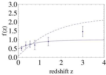
Figure 1: The observed values of the growth rate $f_{obs}$ with $1\sigma$ uncertainty are plotted by the dots with error bars. The theoretical growth rate $f_{th}$ evolve with the redshift $z$ for $\Lambda\textmd{CDM}$ model (solid line) and for the $\Lambda(t)\textmd{CDM}$ (dashed line).

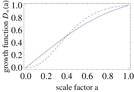
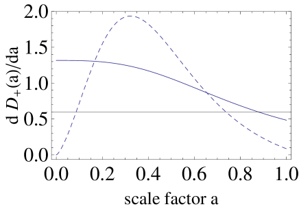
Figure 2: $D_{+}(a)$ vs. $a$ for $\Lambda\textmd{CDM}$ model (solid line) with $\Omega_{m0}=0.27$ and $\Lambda(t)\textmd{CDM}$ model (dashed line) with $\Omega_{m0}=0.27$ and $\beta=4.407$ on the left. The right panel shows $dD_{+}(a)/da$ scales with the scale factor $a$: the solid line is for $\Lambda\textmd{CDM}$ model; the dashed line is for $\Lambda(t)\textmd{CDM}$ model. The values of the cosmological parameter $\Omega_{m0}=0.27$ and the Hubble constant $H_{0}=70.5km/s/Mpc$ are taken by ref:WMAP5 .

Then, the evolutions of growth function $D_{+}(a)$ and its change rate $dD_{+}(a)/da$ as a function of the scale factor have been plotted in FIG.2. From FIG.2, we can see the growth function in $\Lambda(t)\textmd{CDM}$ model is different from that in $\Lambda\textmd{CDM}$ model for the presence of time varying vacuum energy. And it’s found that $D_{+}(a)$ is a little smaller than $D_{\Lambda}$ at $a<0.4$ in the left panel, then there is a trend that the growth function in $\Lambda(t)CDM$ model keeps larger than $D_{\Lambda}$ until now. In the right panel of FIG. 2, it’s found that when $a<0.16$ and $a>0.65$, the rate of change in the growth function $D_{+}(a)$ in $\Lambda(t)\textmd{CD}M$ model is slower than that in $\Lambda\textmd{CDM}$ model, but quicker than the change rate of $D_{\Lambda}$ in $\Lambda\textmd{CDM}$ model with the scale factor ranges $0.16<a<0.65$. And we can find that the increasing rate of the growth function $D_{\Lambda}(a)$ appears to be more and more small along all the scale factor. The right panel shows that there exists an upward trend in the increasing rate of the growth function $D_{+}(a)$ of $\Lambda(t)\textmd{CDM}$ model till $a=0.3$, then it gradually starts to decrease. In FIG.1 and FIG. 2, it’s indicated that there is much discrepancy between the structure growth history in the two models.

III Theory of ISW effect and angular power spectrum

In this section, we give a brief review on ISW effect and its detection, and calculate its angular power spectrum. The ISW effect arises from a time-dependent gravitational potential at late time when dark energy dominates in the universe. The CMB temperature perturbation caused by ISW effect ref:ISW2 is expressed by

$$\frac{\Delta T}{T_{CMB}}\equiv 2\int d\tau\frac{\partial\Phi}{\partial\tau}=-2\int_{0}^{\chi_{H}}d\chi a^{2}H(a)\frac{\partial\Phi}{\partial a},$$ (16)

where $\tau$ and $\chi$ are respectively the conformal time and comoving distance, which are related by $d\chi=-d\tau$. $\Phi$ denotes the gravitational potential, which is related to dark matter perturbation $\delta$ according to Poisson equation on sub-horizon scales:

$$\nabla^{2}\Phi(x)=\frac{a^{2}\rho_{m}(a)\delta(x)}{2},$$ (17)

Carrying out Laplace transform for the two sides of equation (17) and taking the dimensionless dark matter density $\Omega_{m}(a)$ into consideration, we obtain:

$$\Phi(k,a)=-\frac{3}{2}a^{2}H^{2}(a)\Omega_{m}(a)\frac{\delta(k,a)}{k^{2}}.$$ (18)

Substituting the above equation into equation (16), we are able to write down the CMB temperature perturbation coming from ISW effect:

$$\frac{\Delta T}{T_{CMB}}=3H_{0}^{2}\int_{0}^{\chi_{H}}d\chi a^{2}H(a)\frac{d\zeta(a)}{da}\frac{\delta(k,a=1)}{k^{2}},$$ (19)

where the redefined function $\zeta(a)=a^{2}E^{2}(a)\Omega_{m}(a)D_{+}(a)$ is used.

From equation (19), we can see that the source term of ISW effect depends on the following three quantities: the Hubble function $H(a)$, the dimensionless matter density $\Omega_{m}(a)$ and growth function $D_{+}(a)$, all of which are affected by the dark matter production term as we have mentioned in section II.

From the observation point of view, ISW effect leads to these ”new” temperature anisotropies, smaller than those produced at the last scatting surface. So there are many difficulties in directly detecting this effect apart from primary CMB temperature anisotropies. Now, this embarrassment is solved by searching for the cross-correlation between ISW temperature and LSS observations, which include the galaxies sample ref:SDSSmain ; ref:galaxies , quasars sample ref:SDSSquasars , and Luminous Red Galaxies (LRG)ref:SDSSLRG from SDSS, the radio galaxy catalogue from the NRAO VLA Sky Survey (NVSS) ref:NVSS , the infrared catalogue from two Micron All-Sky Survey (2MASS) ref:2MASS , and the X-ray catalogue from the High Energy Astrophysical Observatory (HEAO) ref:HEAO . Here, we use the samples from SDSS and NVSS, which span different redshift ranges. The more detailed presentation on the characteristics of all the samples are given in Ref. ref:densitycontrast ; ref:LSS3 . The observed galaxies density contrast will be ref:densitycontrast ; ref:LSS3 :

$$\delta_{g}=\int b(z)\frac{dN}{dz}\delta(z)dz=\int f(z)\delta(z)dz,$$ (20)

where $\frac{dN}{dz}$ is the selection function of the survey, $b(z)$ is galaxy bias relating the visible matter distribution $\delta_{g}$ to the underlying dark matter $\delta(z)$, which is either a constant or time-evolving with a parameterized form ref:bias . Here we adopt that it is scale independent for simplicity.

We use the approximate function of the redshift distribution of the observed samples released by ref:densitycontrast ; ref:LSS3 ; ref:ISW2 ; ref:RedD ; ref:sample :

$$f_{SDSS}(z)=b(z)\frac{dN}{dz}=b_{g}\frac{\gamma}{\Gamma((m+1)/\gamma)}\frac{z^{m}}{z_{0}^{m+1}}\exp\left[-\left(\frac{z}{z_{0}}\right)^{\gamma}\right],$$ (21)

$$f_{NVSS}(z)=b(z)\frac{dN}{dz}=b_{eff}\frac{\alpha^{\alpha+1}}{z_{\ast}^{\alpha+1}\Gamma(\alpha)}z^{\alpha}e^{-\alpha z/z_{\ast}},$$ (22)

where the parameters can be obtained according to the observation of the galaxy number density after we have selected a certain form of redshift distribution. For the SDSS galaxies sample with the redshift range $0.1<z<0.9$, the best fittings of parameters in equation (19) are given by $z_{0}=0.113$, $\gamma=1.197$ and $m=3.457$ with a median redshift of $z_{med}=0.32$ and a constant bias $b_{g}=1$ in Ref. ref:densitycontrast . For the NVSS sample with a little wider redshift range, the best values of parameters in equation (20) are given by the effective bias $b_{eff}=1.98$, $z_{\ast}=0.79$ and $\alpha=1.18$ in Ref. ref:LSS3 . For the SDSS quasars sample with the redshift between 0.065 and 6.075, it’s found that $z_{0}=1.9$, $\gamma=2.2$ and $m=2$ and its median redshift $z_{med}\sim 1.8$ref:sample . With these best fit parameters, the normalized redshift probability distributions of the SDSS galaxies and quasars sample and NVSS sample are shown together in FIG.3.

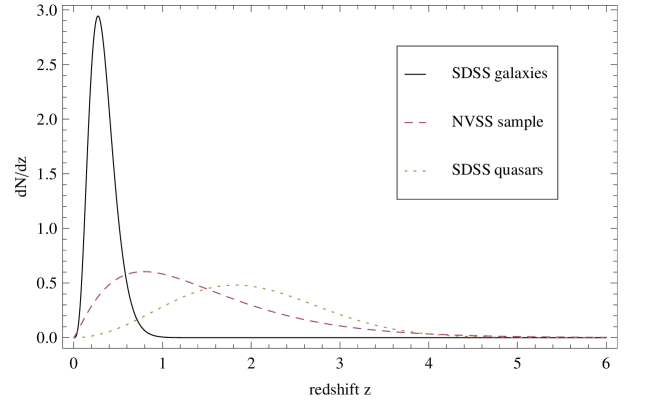
Figure 3: the theoretical redshift distributions d N/d z of three samples with different redshift ranges.

Introducing the weight function $W_{T}(\chi)$ and $W_{g}(\chi)$ as follows ref:ISW2 :

$$W_{T}(\chi)=3a^{2}H(a)\frac{d\zeta(a)}{da},$$ (23)

$$W_{g}(\chi)=H(a)b(a)\frac{dN}{dz}D_{+}(a),$$ (24)

the line of sight integral for ISW temperature perturbation $\Delta T/T_{CMB}$ and the density contrast of observed galaxies $\delta_{g}$ can be written as:

$$\frac{\Delta T}{T_{CMB}}=\int_{0}^{\chi_{H}}d\chi W_{T}(\chi)\frac{H_{0}^{2}\delta(k,a=1)}{k^{2}},$$ (25)

$$\delta_{g}=\int_{0}^{\chi_{H}}d\chi W_{g}(\chi)\delta(k,a=1),$$ (26)

which allow the expressions for the ISW-auto spectrum $C_{TT}(l)$, the ISW-cross spectrum $C_{Tg}(l)$ and the observed galaxies-auto spectrum $C_{gg}(l)$ to be written in a compact notation, applying the Limber-projection ref:Limber in the flat-sky approximation, for simplicity:

$$C_{TT}(l)=\int_{0}^{\chi_{H}}d\chi\frac{W_{T}(\chi)^{2}}{\chi^{2}}\frac{H_{0}^{4}P_{\delta\delta}(k=l/\chi)}{k^{4}},$$ (27)

$$C_{Tg}(l)=\int_{0}^{\chi_{H}}d\chi\frac{W_{T}(\chi)W_{g}(\chi)}{\chi^{2}}\frac{H_{0}^{2}P_{\delta\delta}(k=l/\chi)}{k^{2}},$$ (28)

$$C_{gg}(l)=\int_{0}^{\chi_{H}}d\chi\frac{W_{g}(\chi)^{2}}{\chi^{2}}P_{\delta\delta}(k=l/\chi),$$ (29)

where $P_{\delta\delta}(k)$ is the present matter power spectrum. Here we take $P(k)\propto k^{n_{s}}T^{2}(k)$ and it can be normalized by $\sigma_{8}=0.8$. $T(k)$ is the transfer function, and we adopt its fitting form by ref:ISW2 ; ref:transferfunction :

$$T(q\equiv k/\Gamma hMpc^{-1})=\frac{\ln[1+2.34q]}{2.34q}\left[1+3.89q+(16.2q)^{2}+(5.47q)^{3}+(6.71q)^{4}\right]^{-0.25},$$ (30)

where the dimensionless quantity $\Gamma=\Omega_{m0}h$.

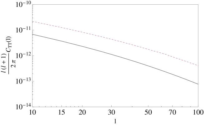
Figure 4: the ISW-auto power spectrum $C_{TT}$ vs. multipole order $l$ for $\Lambda\textmd{CDM}$ model (solid line) and $\Lambda(t)\textmd{CDM}$ model (dashed line).

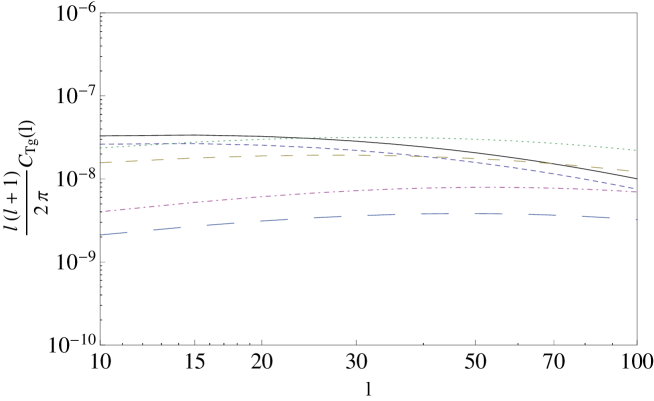
Figure 5: the ISW-cross power spectrum $C_{Tg}$ vs. multipole order $l$ for $\Lambda\textmd{CD}M$ model: the short-dashed line is for the SDSS galaxies sample; the dashed line is for the NVSS sample; the long-dashed line is for the SDSS quasars sample; and $\Lambda(t)\textmd{CDM}$ model: the black line is for the SDSS galaxies sample; the dotted line is for the NVSS sample; the dot-dashed line is for the SDSS quasars sample.

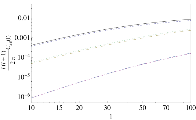
Figure 6: the observed galaxies-auto power spectrum $C_{gg}$ vs. multipole order $l$ for $\Lambda\textmd{CDM}$ model: the short-dashed line is for the SDSS galaxies sample; the dashed line is for the NVSS sample; the long-dashed line is for the SDSS quasars sample; and $\Lambda(t)\textmd{CDM}$ model: the black line is for the SDSS galaxies sample; the dotted line is for the NVSS sample; the dot-dashed line is for the SDSS quasars sample.

As shown in FIG. 4, 5, 6, the power spectrums, including the ISW-auto power spectrum $C_{TT}(l)$, the ISW-cross power spectrum $C_{Tg}(l)$, and the observed galaxies-auto power spectrum $C_{gg}(l)$, have been affected due to the presence of the time varying vacuum energy. The amplitudes of the ISW-auto power spectrums and ISW-cross power spectrums in $\Lambda(t)\textmd{CDM}$ model are a few higher than those in the cosmological constant model. There is a minor difference between the observed galaxies-auto power spectrum amplitudes in the $\Lambda(t)\textmd{CDM}$model and the $\Lambda\textmd{CDM}$ model. The FIG.5 and FIG. 6 show respectively the ISW-cross power spectrum $C_{Tg}(l)$ and the observed galaxies-auto power spectrum $C_{gg}(l)$ are related to the observed samples with different redshift ranges. In FIG. 5, it’s found that the differences of the ISW-cross power spectrum $C_{Tg}(l)$ in the two models become larger when the observed galaxies with wider redshift ranges are used. Since the total CMB temperature-auto power spectrum in $\Lambda\textmd{CDM}$ model is still consistent with the observational results from WMAP, a few increase in the ISW-auto power spectrum $C_{TT}(l)$ in $\Lambda(t)\textmd{CDM}$ model may lead to the trouble between the total CMB temperature-auto power spectrum in $\Lambda(t)\textmd{CDM}$ model and the observational results from WMAP. As we have mentioned, it’s difficult to directly detect the amplitude of the ISW-auto power spectrum $C_{TT}(l)$ apart from the total CMB temperature anisotropies. However, it’s lucky that the ISW-cross power spectrum $C_{Tg}(l)$ provides an effective measurement for the ISW effect. In FIG.7, we show the observational data of the ISW-cross power spectrum $C_{Tg}$ between ISW temperature and the radio galaxy catalogue from the NVSS and its theoretical evolutions in $\Lambda\textmd{CDM}$ model and $\Lambda(t)\textmd{CDM}$ model. It’s found that the ISW-cross power spectrum $C_{Tg}$ in $\Lambda(t)\textmd{CDM}$ model is still consistent with the observational results within $1\sigma$ errors. Although the amplitude of the ISW-auto power spectrum $C_{TT}(l)$ in $\Lambda(t)\textmd{CDM}$ model is a few higher than that in $\Lambda\textmd{CDM}$ model, its contribution to the total CMB temperature power spectrum is still small and don’t bring about the disagreement between WMAP observations and the total CMB temperature power spectrum. So, the WMAP measurements can not rule the $\Lambda(t)\textmd{CDM}$ model out at present. In addition, FIG.8 shows the comparison of the observational data of the observed galaxies-auto power spectrum $C_{gg}$ from the NVSS and the theoretical evolutions of $C_{gg}$ in the two models.

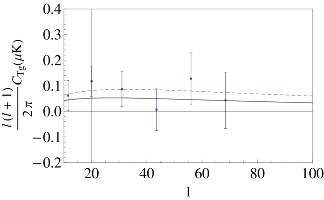
Figure 7: Comparison of the observational data of the ISW-cross power spectrum $C_{Tg}$ between ISW temperature and the radio galaxy catalogue from the NVSS ref:LSS3 and the theoretical evolutions of $C_{Tg}$: the dots with error bars denote the observed data with its corresponding uncertainty; the solid line is for the $\Lambda\textmd{CDM}$ model; the dashed line is for the $\Lambda(t)\textmd{CDM}$ model. The well-measured temperature $T_{CMB}$ is 2.725K by ref:WMAP5 ; ref:T0 .

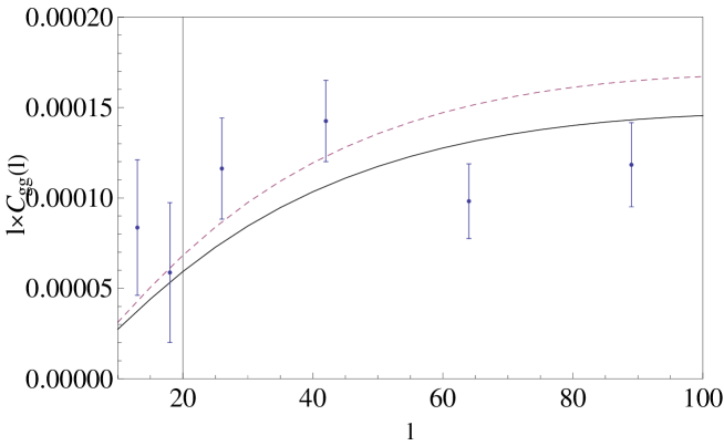
Figure 8: Comparison of the observational data of the observed galaxies-auto power spectrum $C_{gg}$ from the NVSS ref:LSS3 and the theoretical evolutions of $C_{gg}$: the dots with error bars denote the observed data with its corresponding uncertainty; the solid line is for the $\Lambda\textmd{CDM}$ model; the dashed line is for the $\Lambda(t)\textmd{CDM}$ model.

IV Conclusion

In summary, we have calculated the power spectrum of the ISW effect in the time varying vacuum energy model. It’s shown that the source of the ISW effect is not only affected by the different evolutions of the Hubble function $H(a)$ and the dimensionless matter density $\Omega_{m}(a)$, but also by the different growth function $D_{+}(a)$, all of which are changed due to the presence of matter production term in the time varying vacuum model. In FIG. 1 and FIG. 2, it’s seen that the difference between the growth function in $\Lambda(t)\textmd{CDM}$ model and that in $\Lambda\textmd{CDM}$ model is not minor. What’s more, the left panel in FIG. 2 shows there is a crosspoint at $a=0.4$ for the evolutions of the growth function in two models. The growth function in $\Lambda\textmd{CDM}$ model is greater than that in $\Lambda(t)\textmd{CDM}$ model before $a=0.4$. When $a>0.4$, the growth function in $\Lambda\textmd{CDM}$ model is smaller than that in $\Lambda(t)\textmd{CDM}$ model. However, since the ISW effect is calculated by integrating time-dependent gravitational potential from the time of last scattering to the present, the difference of the ISW effect caused by the difference of the growth function in the two models within the scale factor ranges $[0.4,1]$ can partly counteract that caused by the discrepancy in their growth functions at $a<0.4$ though the integration. Therefore, the difference of the ISW effect in $\Lambda(t)\textmd{CDM}$ model and $\Lambda\textmd{CDM}$ model is lessened to a certain extent due to the integrated effect. As shown in FIG. 5, there is not much discrepancy between the availably observed quantities $C_{Tg}$ in the two models for the SDSS galaxies and the sample from NVSS. For the SDSS quasars with high redshift, the amplitudes of the ISW-cross power spectrum in $\Lambda(t)\textmd{CDM}$ model and $\Lambda\textmd{CDM}$ model obviously decrease. However, the relative discrepancy between ISW-cross power spectrums in $\Lambda(t)\textmd{CDM}$ model and $\Lambda\textmd{CDM}$ model for the SDSS quasars is larger than those for the SDSS galaxies and the sample from NVSS. Therefore, at present the ISW effect is weaker than the growth history in distinguishing $\Lambda\textmd{CDM}$ model and $\Lambda(t)\textmd{CDM}$ model. However, it’s worth expecting the observational data of the ISW-cross power spectrum for the observed galaxies with high redshift in the future.

References

- (1) A. G. Riess et al., Astron. J. 116 1009 (1998) [astro-ph/9805201].
- (2) S. Perlmutter et al., Astrophys. J. 517 565 (1999) [astro-ph/9812133].
- (3) D. N. Spergel et al., Astrophys. J. Supp. 148 175 (2003) [astro-ph/0302209].
- (4) D. N. Spergel et al., Astrophys. J. Supp. 170 377 (2007) [astro-ph/0603449].
- (5) M. Tegmark et al., Phys. Rev. D 69 103501 (2004) [astro-ph/0310723].
- (6) M. Tegmark et al., Astrophys. J. 606 702 (2004) [astro-ph/0310725].
- (7) A. Einstein, Sitzungsber. Preuss. Akad. Wiss. Berlin (Math. Phys. ) 1917 (1917) 142.
- (8) V. Sahni and A. A. Starobinsky, Int. J. Mod. Phys. D 9 (2000) 373. E. J. Copeland, M. Sami and S. Tsujikawa, Int. J. Mod. Phys. D 15 (2006) 1753.
- (9) B. Ratra and P. J. E. Peebles, Phys. Rev. D. 37 (1988) 3406. M. S. Turner and M. White, Phys. Rev. D 56 (1997) 4439. R. R. Caldwell, R. Dave and P. J. Steinhardt, Phys. Rev. Lett. 80 (1998) 1582. P. J. Steinhardt, M. L. Wang and I. Zlatev, Phys. Rev. D 59 (1999) 123504. V. Sahni and A. A. Starobinsky, Int. J. Mod. Phys. D 9 (2000) 373.
- (10) R. R. Caldwell, Phys. Lett. B 545 (2002) 23. N. N. Weinberg, Phys. Rev. Lett. 91 (2003) 071301. S. Nojiri and S. D. Odintsov, Phys. Rev. D 72 (2005) 023003.
- (11) B. Feng, X. L. Wang and X. M. Zhang, Phys. Lett. B 607 (2005) 35. Z. K. Guo, Y. S. Piao, X. N. Zhang and Y. Z. Zhang, Phys. Lett. B 608 (2005) 177.
- (12) A. Y. Kamenshchik, U. Moschella and V. Pasquier, Phys. Lett. B 511 (2001) 265. M. C. Bento, O. Bertolami and A. A. Sen, Phys. Rev. D 66 (2002) 043507. M. C. Bento, O. Bertolami, M. J. Reboucas and P. T. Silva, Phys. Rev. D 73 (2006) 043504. J. B. Lu, Phys. Lett. B 680 (2009) 404. J. B. Lu, Y. X. G, and L. X. Xu, Eur. Phys. J. C 63 (2009) 349.
- (13) M. Li, Phys. Lett. B 603 (2004) 1. Y. G. Gong, Phys. Rev. D 70 (2004) 064029. B. Wang , E. Abdalla and R. K. Su, Phys. Lett. B 611 (2005) 21.
- (14) E. Komatsu et al., Astrophys. J. Suppl. 180 (2009) 330.
- (15) J. S. Alcaniz, Braz. J. Phys. 36 (2006) 1109. S. Basilakos, arXiv: 0901.3195. J. M. F. Maia and J. A. S. Lima, Phys. Rev. D 65 (2002) 083513. V. Sahni, Class. Quant. Grav. 19 (2002) 3435.
- (16) S. Basilakos, M. Plionis and J. Sola, arXiv: 0907.4555.
- (17) I. L. Shapiro and J. Sol, J. High Energy Phys. 02 (2002) 006. I. L. Shapiro and J. Sol, Phys. Lett. B 475 (2000) 236. L. X. Xu, arXiv: 0906.1113.
- (18) R. K. Sachs and A. M. Wolfe, Astrophys. J. 147 (1967) 73.
- (19) J. Garriga, L. Pogosian and T. Vachaspati, Phys. Rev. D 69 (2004) 063511.
- (20) T. Giannantonio, R. Scranton, R. G. Crittenden, R. C. Nichol, S. P. Boughn, A. D. Myers and G. T. Richards, Phys. Rev. D 77 (2008) 123520.
- (21) S. Ho, C. M. Hirata, N. Padmanabhan, U. Seljak and N. Bahcall, Phys. Rev. D 78 (2008) 043519;
- (22) B. R. Granett, M. C. Neyrinck and I. Szapudi, Astrophys. J. 683 (2008) L99-L102.
- (23) B. R. Granett, M. C. Neyrinck and I. Szapudi, Astrophys. J. 701 (2009) 414-422.
- (24) S. Basilakos, Mon. Not. Roy. Astron. Soc., 395 (2009) 2347.
- (25) R. C. Arcuri and I. Waga, Phys. Rev. D 50 (1994) 2928. K. Y. Kim, H. W. Lee, and Y. S. Myung, arXiv: 0805.3941.
- (26) E. Hawkins et al., Mon. Not. R. Astron. Soc., 346 (2003) 78, astro-ph/0212375; L. Verde et al., Mon. Not. R. Astron. Soc., 335 (2002) 432, astro-ph/0112161; E. V. Linder, Astropart. Phys. 29 (2008) 336, arXiv: 0709.1113 [astro-ph].
- (27) M. Tegmark et al., SDSS Collaboration, Phys. Rev. D 74 (2006) 123507, astroph/ 0608632.
- (28) N. P. Ross et al., Mon. Not. Roy. Astron. Soc. 381 (2007) 573, astro-ph/0612400.
- (29) L. Guzzo et al., Nature 451 (2008) 541, arXiv:0802.1944.
- (30) J. da Angela et al., astro-ph/0612401.
- (31) P. McDonald et al., SDSS Collaboration, Astrophys. J. 635 (2005) 761, astro-ph/ 0407377.
- (32) B. M. Schaefer, arXiv: 0803.2239. D. Sapone, and M. Kunz, Phys. Rev. D 80 (2009) 083519.
- (33) J. K. Adelman-McCarthy et al. [SDSS Collaboration], Astrophys. J. Suppl. 175 (2008) 297-313, arXiv:0707.3413 [astro-ph]. D. G. York et al. [SDSS Collaboration], Astron. J. 120 (2000) 1579.
- (34) A. Refregier, and the DUNE collaboration, Exper. Astron. 23 (2009) 17-37, arXiv: 0802.2522.
- (35) G. T. Richards et al., Astrophys. J. Suppl. 180 (2009) 67. G. T. Richards et al., [SDSS Collaboration], Astrophys. J. Suppl. 155 (2004) 257.
- (36) A. Collister et al., Mon. Not. Roy. Astron. Soc. 375 (2007) 68. C. Blake, A. Collister, S. Bridle and O. Lahav, Mon. Not. Roy. Astron. Soc. 374 (2007) 1527-1548, arXiv:astro-ph/0605303.
- (37) J. J. Condon et al., Astrophys. J. 115 (1998) 1693.
- (38) T. H. Jarrett, T. Chester, R. Cutri, S. Schneider, M. Skrutskie and J. P. Huchra, Astron. J. 119 (2000) 2498-2531. M. F. Skrutskie et al., Astron. J. 131 (2006) 1163.
- (39) E. A. Boldt, Phys. Rept. 146 (1987) 215. S. P. Boughn, R. G. Crittenden and N. G. Turok, New Astron. 3 (1998) 275. S. P. Boughn, R. G. Crittenden and G. P. Koehrsen, Astrophys. J. 580 (2002) 672.
- (40) B. M. Schaefer, M. Douspis and N. Aghanim, arXiv: 0903.4288.
- (41) M. Douspis, P. G. Castro, C. Caprini and N. Aghanim, arXiv: 0802.0983.
- (42) J. Q. Xia, M. Viel, C. Baccigalupi and S. Matarrese, arXiv: 0907.4753.
- (43) D. N. Limber, Astrophys. J. 119 (1954) 655. N. Kaiser, Astrophys. J. 388 (1992) 272.
- (44) S. Dodelson; MODERN COSMOLOGY (Academic Press).
- (45) J. C. Mather et al., Astrophys. J. 512 (1999) 511.