An approach to the formalism of the Standard Model of Particle Physics

Abstract

So far, the Standard Model of particle physics (SM) describes the phenomenology observed in high energy physics. In the Large Hadron Collider (LHC) is expected to find the Higgs boson, which is an essential part of SM; also expects to see new particles or deviations from the SM, which would be evidence of other truly fundamental theory. Consequently, a clear understanding of the SM and, in general, quantum field theory is of great importance for particle physics, however, students face a formalism and a set of concepts with which they are unfamiliar. This paper shows how to make an approach to SM to introduce students to the formalism and some fundamental concepts.

I Introduction

A problematic situation with the introduction in the study of the Standard Model of Particle Physics (SM), which constitutes the main motivation of this article, is the fact that usually the process of formalizing the model is one of the aspects that cause difficulties to students. However, it is intended to formalize knowledge, but what is sought is based on a series of paradigms and rules for creating a solid foundation on which to work, which can be modified when necessary Kuhn .

In this context is the SM which describes, with subtle precision and mathematical elegance, all known particles and interactions, except gravity. All model predictions have been corroborated, however, the Large Hadron Collider (LHC) is expected to be a new physics or physics beyond the SM, in the TeV scale, which can manifest itself in two ways: through signals involved in the production of new particles or deviations from SM predictions. Consequently, a clear understanding of the SM and, in general, quantum field theory is of great importance for particle physics, this paper shows how to make an approach to SM to introduce students quickly in the formalism and basic concepts.

II Reviewing some basic concepts

II.1 Fermion-boson interaction

Everything that exists in nature is made of material particles (called fermions) which interact, either because they decay or because they respond to a force due to the presence of another particle. The decay of a fermion into a different one is explained by the action of a third call mediator boson. Similarly, the interaction of two particles through the fields that originate, can be interpreted considering that the two particles exchange a mediator boson. In quantum mechanics fermions or bosons can be represented by fields with some intrinsic properties. The interaction process is an exchange of energy and momentum, between fields, governed by laws of conservation of intrinsic quantities (e.g., some kind of charge).

II.1.1 Mechanical model

To explain the interaction between a fermion and a boson, we use a mechanical model consisting of two coupled mass-spring systems. The Lagrangian of the system is given by:

$$L=\frac{p_{1}^{2}}{2m_{1}}+\frac{p_{2}^{2}}{2m_{2}}-\frac{1}{2}k.V(x_{1},x_{2}).$$

The kinetic energy of the first oscillator can represent a free fermion (e.g., electron), the second oscillator a free boson (e.g., electromagnetic field) and potential energy, the fermion-boson interaction (e.g., electron in electromagnetic field). Note that the interaction is characterized by a constant (spring constant). Therefore, we will always have three classes of Lagrangians: the free fermion, the free boson and fermion-boson interaction. It is clear that the interaction occurs at a predetermined time, called mean-lifetime.

II.1.2 Electromagnetic model

In electromagnetic theory, the Lagrangian for a free particle of mass $m$ and an free electromagnetic field represented for a potential, $\overrightarrow{A}$, in vacuum, is written as

$$L_{\textrm{free}}=\frac{p^{2}}{2m}+\frac{1}{8\pi}\int d^{3}x\left(\frac{1}{c^{2}}\left|\frac{\partial\overrightarrow{A}}{\partial t}\right|^{2}+\left|\overrightarrow{\nabla}\times\overrightarrow{A}\right|^{2}\right).$$ (1)

The introduction of the interaction reduces simply to the replacement of ordinary momentum by canonical momentum (as is usual in electrodynamics): $\overrightarrow{P}\rightarrow\overrightarrow{p}+\frac{q}{c}\overrightarrow{A}$. Substituting we obtain the Lagrangian for a particle interacting:

$$L_{\textrm{with interaction}}=L_{\textrm{free}}+\frac{q}{2mc}\overrightarrow{A}.\left(2\overrightarrow{p}+\frac{q}{c}\overrightarrow{A}\right).$$

II.1.3 Quantum-mechanical model

In the formalism of relativistic quantum mechanics a free particle can be represented by a field called spinor,$\Psi=\Psi(x^{\mu})$. In the continuum, the Lagrangian ($L=L(q,\dot{q})$) is replaced by a Lagrangian density ($\mathcal{L}$), the generalized coordinates ($q$) by the fields ($\Psi$) and the generalized velocities ($\dot{q}=dq/dt$) by the field gradient ($\partial_{\mu}\Psi=\partial\Psi/\partial x^{\mu}$): $\mathcal{L}=\mathcal{L}(\Psi,\partial_{\mu}\Psi)$. For simplicity, in what follows, we use natural units where $\hbar=1$ and $c=1$. The Lagrangian density for a free particle and an electromagnetic field, equivalent to the equation (1), fully consistent with the principles of quantum mechanics and special relativity ($v\simeq c$), is given by:

$$\mathcal{L}_{\textrm{free}}=\overline{\Psi}(i\gamma^{\mu}\partial_{\mu}-m)\Psi-\frac{1}{4}F_{\mu\nu}F^{\mu\nu},$$ (2)

where $\overline{\Psi}$ is defined as $\overline{\Psi}=\Psi^{\dagger}\gamma^{0}$ and $F_{\mu\nu}=\partial_{\mu}A_{\nu}-\partial_{\nu}A_{\mu}$. The first term is called the Dirac Lagrangian. In order to introduce the interaction we replace the ordinary momentum $p_{\mu}$ by canonical momentum $P_{\mu}\rightarrow p_{\mu}+qA_{\mu}$, where $q$ is the coupling constant, which in this case corresponds to the charge. In language operator the momentum of the particle is given by $p_{\mu}=-i\partial_{\mu}$, and $P_{\mu}=-iD_{\mu}$, then, the introduction of the interaction for the relativistic quantum particle interacting with the field, translates to replace the normal derivative by the covariant derivative in the Lagrangian, $D_{\mu}\rightarrow\partial_{\mu}-iqA_{\mu}$:

$$\mathcal{\mathcal{L}_{\textrm{{with interaction}}}}=\mathcal{L}_{\textrm{free}}+q\overline{\Psi}\gamma^{\mu}\Psi A_{\mu},$$ (3)

here, $J^{\mu}=q\overline{\Psi}\gamma^{\mu}\Psi$ is a current satisfying: $\partial_{\mu}J^{\mu}=0$, indicating that it is a conserved quantity Quigg .

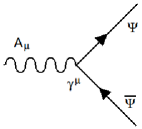
Figure 1: Feynman diagram for $\mathcal{\mathcal{L}_{\textrm{i}}}=q\overline{\Psi}\gamma^{\mu}\Psi A_{\mu}$

The interaction terms can be represented by Feynman diagrams, we have six possibilities: creation and annihilation of an electron-positron pair, or absorption of a photon by an electron or a positron.

II.2 Quantum operators

Consider the operator rotation, $R$, where an infinitesimal rotation is defined by $R(\delta\theta)\left|\Psi(\theta)\right\rangle=\left|\Psi(\theta-\delta\theta)\right\rangle$; when we expand the right side in a Taylor series around $\theta$, we get, $R(\delta\theta)\left|\Psi(\theta)\right\rangle=\left(I-iJ\delta\theta\right)\left|\Psi(\theta)\right\rangle$. where the $J$ operator is called the generator of rotations. Consequently, a rotation is given by an infinite number of infinitesimal rotations Lichtenberg :

$$R(\theta)=\underset{N\longrightarrow\infty}{l\acute{\imath}m}\left[I-iJ\left(\frac{\theta}{N}\right)\right]^{N}=e^{-iJ\theta}.$$ (4)

It is not difficult to demonstrate that in order to conserve the probability the $R$ operator must be unitary, $R^{\dagger}R=RR^{\dagger}=I$; this is true only if your generator is hermitian $J=J^{\dagger}$.

Symmetry	Operator	Generator	Conservation law
Temporary evolution	$e^{-iHt}$	$H$	Energy
Translation	$e^{ipx}$	$p$	Momentum
Rotation	$e^{-iJ\theta}$	$J$	Angular Momentum
4D Rotation	$e^{ip_{\mu}x^{\mu}}$	$p_{\mu}$	4-momentum
Gauge	$e^{-iq\alpha(x)}$	$q$	Charge

Table 1: Some quantum operators, symmetry and conservation laws.

All operators of quantum mechanics can be constructed in the same way and have the form of a rotation transformation. Noether’s theorem establishes that if an action is invariant under a transformation group (symmetry), there are one or more quantities (constants of motion) which are associated with these transformations, in other words, to each symmetry corresponds a conservation law Goldstein . We see that each operator has a generator, and the generators belong to a particular Lie group. The commutators of these generators are linear combinations that define the group algebra, meaning the commutation of two generators of the group produces a third generator of the same group; this can be shown using the definition (4) Townsend .

II.3 Local phase invariance

We can change the phase of all the fields that represent the particles (local phase change), $\Psi\rightarrow\Psi^{\prime}=e^{-iq\alpha(x)}\Psi,$ note that $\alpha$ is a function that depends on the coordinates $\alpha=\alpha(x)$ and $q$ is the generator. In this case the Dirac Lagrangian ceases to be invariant:

$$\mathcal{L}_{D}=\overline{\Psi}(i\gamma^{\mu}\partial_{\mu}-m)\Psi+q\overline{\Psi}\gamma^{\mu}\Psi\partial_{\mu}\alpha\left(x\right).$$

We can demand that the Lagrangian is invariant under local phase transformation, by removing how the additional term that appears. By making the particle to interact with potential $A_{\mu}$, see equation (3), the Lagrangian is composed of three terms, the Lagrangian particle to which is added a term due to the potential and another term due to local phase change:

$$\mathcal{L}_{D} = \overline{\Psi}(i\gamma^{\mu}D_{\mu}-m)\Psi+q\overline{\Psi}\gamma^{\mu}\Psi\partial_{\mu}\alpha\left(x\right)$$

$$= \overline{\Psi}(i\gamma^{\mu}\partial_{\mu}-m)\Psi+q\overline{\Psi}\gamma^{\mu}\Psi A_{\mu}+q\overline{\Psi}\gamma^{\mu}\Psi\partial_{\mu}\alpha\left(x\right).$$

We can calibrate the potential in such a way that the term of change of phase is cancelled:

$$A_{\mu}\rightarrow A_{\mu}-q\partial_{\mu}\alpha(x),$$ (5)

then

$$\mathcal{L}_{D}=\overline{\Psi}(i\gamma^{\mu}D_{\mu}-m)\Psi.$$ (6)

We see that this Lagrangian, which represents an interacting particle with a potential; is invariant under a local phase change, if the potential is calibrated (5). The fields represented by such calibrated potentials are called gauge fields.

III Yang-Mills fields

Consider that we have $n$ fields represented by potentials, $A_{\mu}^{a}$ $(a=1,2,3,\ldots,n)$, the covariant derivative takes the form: $D_{\mu}=\partial_{\mu}-iq_{a}A_{\mu}^{a}$ and gauge invariance occurs under the local transformation $\Psi\rightarrow\Psi^{\prime}=e^{-iq_{a}\alpha^{a}(x)}\Psi$. By means of the operator of change of phase the representation of the Lie group can be obtained doing $q_{a}=gT_{a}$, where $g$ corresponds to the coupling constant and $T_{a}$ to the group generators, i.e., $\Psi\rightarrow\Psi^{\prime}=e^{-igT_{a}\alpha^{a}(x)}\Psi$. In this way we associate a potential $A_{\mu}^{a}$ a group represented by its generator $T_{a}$. The commutators of the generators of a Lie group is a linear combination of generators: $\left[T_{a},T_{b}\right]=if_{abc}T^{c}$, where the coefficients of the linear combination $f_{abc}$, are the structure constants of the group.By analogy with the electromagnetic field tensor, the field tensor $F_{\mu\nu}^{a}$ is defined as generalized as:

$$iq_{a}F_{\mu\nu}^{a}=\left[D_{\nu},D_{\mu}\right].$$ (7)

Substituting the covariant derivative and commutator of the generators of the group is obtained:

$$F_{\mu\nu}^{a}=\partial_{\mu}A_{\nu}^{a}-\partial_{\nu}A_{\mu}^{a}+gf_{bc}^{a}A_{\mu}^{b}A_{\nu}^{c},$$ (8)

we see that the first two terms of this expression correspond to a tensor analogous to the electromagnetic field and the last term is the fact that generators are not abelian group; this allows to create no-abelians gauge theories or Yang-Mills theories Yang-Mills . With the gauge field tensor is constructed from Yang-Mills Lagrangian for the free field:

$$\mathcal{L}=-\frac{1}{4}F_{\mu\nu}^{a}F_{a}^{\mu\nu},$$ (9)

note its similarity to the free electromagnetic field Lagrangian (2).

IV The Standard Model

IV.1 Strong Interaction

To build the model for the strong interaction we propose a Lagrangian invariant under local gauge transformations of the $SU(3)_{C}$ group, the subscript $C$ indicates that the transformations only act on particles with color charge. The strong interaction is represented by means eight gauge fields for gluons $G_{\mu}^{a}$ $(a=1,2,\ldots,8)$ and each of these fields is associated generators $T_{a}=\lambda_{a}/2$, being $\lambda_{a}$ the Gell-Mann matrices: $\Psi\rightarrow\Psi^{\prime}=e^{-ig_{s}T_{a}\alpha^{a}(x)}\Psi$. The coupling constants of the fields with gluons are $q_{a}=g_{s}T_{a}$. Lie algebra, is obtained with the following rule of commutation: $\left[T_{a},T_{b}\right]=if_{ab}^{c}T_{c}$, where $f_{ab}^{c}$ it is the structure constant of the $SU(3)$ group. The covariant derivative is given by:

$$D_{\mu}=I\partial_{\mu}-ig_{s}\frac{\lambda_{a}}{2}G_{\mu}^{a}.$$

Applying the definition (7)(8) obtain the tensor field:

$$G_{\mu\nu}^{a}=\partial_{\mu}G_{\nu}^{a}-\partial_{\nu}G_{\mu}^{a}+g_{s}f_{bc}^{a}G_{\mu}^{b}G_{\nu}^{c},$$

and for the free field Lagrangian (9) is

$$\mathcal{L}=-\frac{1}{4}G_{\mu\nu}^{a}G_{a}^{\mu\nu}.$$

IV.2 Electroweak Interaction

A very interesting aspect of SM is that the electromagnetic interactions and weak interactions are combined into a single, so called, electroweak interaction. For electroweak interactions we propose a Lagrangian invariant under local gauge transformations of the $SU(2)_{L}\otimes U(1)_{Y}$ group, the subscript $L$ means that these transformations only act on components of the left chiral fermions and $Y$ is the hypercharge quantum number. Electroweak interactions are represented by four gauge fields $W_{\mu}^{i}$ $(i=1,2,3)$ and $B_{\mu}$. Each of these fields are associated generators $\tau_{i}=\sigma_{i}/2$ of the weak isospin group $SU(2)_{L}$ and $y=IY/2$, corresponding to the $U(1)_{Y}$ group, respectively. Here $\sigma_{i}$ are the Pauli matrices, $I$ the $2\times 2$ unit matrix and $Y$ hypercharge quantum number. The coupling constants of the flavor change with the electroweak field are $q_{i}=g\tau_{i}$ and $q=g^{\prime}y$. The group algebra is given by the following commutation rules: $\left[\tau_{i},\tau_{j}\right]=i\epsilon_{ij}^{k}\tau_{k}$ and $\left[\tau_{i},y\right]=0$, where $\epsilon_{ij}^{k}$ is the constant of structure of the $SU(2)$ group. The covariant derivative is given by:

$$D_{\mu}=I\partial_{\mu}-ig\frac{\sigma_{i}}{2}W_{\mu}^{i}-ig^{\prime}I\frac{Y}{2}B_{\mu}.$$ (10)

Applying again the definition (7)(8) one obtains the tensor field:

$$W_{\mu\nu}^{i} = \partial_{\mu}W_{\nu}^{i}-\partial_{\nu}W_{\mu}^{i}+gf_{jk}^{i}W_{\mu}^{j}W_{\nu}^{k},$$

$$B_{\mu\nu} = \partial_{\mu}B_{\nu}-\partial_{\nu}B_{\mu},$$

note that the gauge fields $W_{\mu}^{i}$ are non-abelian Yang-Mills fields and gauge field $B_{\mu}$ is a abelian field, because the structure constant of the group is zero. For the free field (9) is

$$\mathcal{L}=-\frac{1}{4}W_{\mu\nu}^{i}W_{i}^{\mu\nu}-\frac{1}{4}B_{\mu\nu}B^{\mu\nu}.$$

Performing the matrix operations indicated in the covariant derivative (10) and by means the linear combination of the first two components of the gauge field, $W_{\mu}^{1}$ y $W_{\mu}^{2}$, one can build charged intermediate vector bosons, $W_{\mu}^{+}$ y $W_{\mu}^{-}$:

$$W_{\mu}^{\pm}=\frac{1}{\sqrt{2}}\left(W_{\mu}^{1}\mp iW_{\mu}^{2}\right),$$ (11)

and with the mixture of the third component of the gauge field, $W_{\mu}^{3}$ with the gauge field $B_{\mu}$, the neutral vector boson is obtained $Z_{\mu}^{o}$ and the boson of the electromagnetic field, $A_{\mu}^{o}$ (photon) (superscript $o$ indicates that it is a field with neutral electric charge):

$$\left(\begin{array}[]{c}Z_{\mu}^{o}\\ A_{\mu}^{o}\end{array}\right)=\left(\begin{array}[]{cc}\cos\theta_{w}&-\sin\theta_{w}\\ \sin\theta_{w}&\cos\theta_{w}\end{array}\right)\left(\begin{array}[]{c}W_{\mu}^{3}\\ B_{\mu}\end{array}\right),$$ (12)

where the mixing angle, $\theta_{w}$, called Weinberg angle; which is defined by the ratio of the electroweak coupling constants, $\tan\theta_{w}=g^{\prime}/g$ and the value of the electron charge, $e=g\sin\theta_{w}=g^{\prime}\cos\theta_{w}$, which represents the unification of the weak field with the electromagnetic Quigg . The hypercharge $Y$ is related to the electric charge $Q$ by the Gell-Mann Nishijima relation Gell-Mann : $Q=\tau_{3}+\frac{1}{2}IY$, here $\tau_{3}=\sigma_{3}/2$ it is third generator of the $SU(2)$ group and $Y$ hypercharge quantum number. Substituting these definitions, (11) and (12) in the covariant derivative (10), we obtain:

$$\begin{array}[]{c c c}D_{\mu}&=&I\partial_{\mu}-ieQA_{\mu}^{o}-i\frac{g}{\sqrt{2}}\sigma^{+}W_{\mu}^{+}-i\frac{g}{\sqrt{2}}\sigma^{-}W_{\mu}^{-}\\ &&-i\frac{g}{\cos\theta_{w}}\left(\tau_{3}-Q\sin^{2}\theta_{w}\right)Z_{\mu}^{o},\end{array}$$ (13)

where $Q=\frac{1}{2}\left(\begin{array}[]{cc}Y+1&0\\ 0&Y-1\end{array}\right)$.

IV.3 Fermions

Fields representing fermions can be decomposed into a left and right chiral components: $\Psi=\Psi_{L}+\Psi_{R}$, using chiral projectors $P_{L}=\frac{1}{2}(1-\gamma^{5})$ and $P_{R}=\frac{1}{2}(1+\gamma^{5})$, where $\Psi_{L}=P_{L}\Psi$ and $\Psi_{R}=P_{R}\Psi$.

Fermions, quarks and leptons, are classified into three groups called generations. A generation is formed by quarks and an leptons with different charges, and generations are ordered from the lightest to the heaviest. The left component of the leptons is given by a doublet $\Psi_{Li}=\left(\begin{array}[]{c}\nu_{i}\\ e_{i}\end{array}\right)_{L}$, where $\nu_{i}\equiv\nu_{e},\nu_{\mu},\nu_{\tau}$ and $e_{i}\equiv e,\mu,\tau$; for quarks $\Upsilon_{Li}=\left(\begin{array}[]{c}u_{i}\\ d^{\prime}_{i}\end{array}\right)_{L}$, where $u_{i}\equiv u,c,t$; $d^{\prime}_{i}=V_{ij}d_{j}$ with $V_{ij}$ an element of the Cabibbo-Kobayashi-Maskawa (CKM) matrix and $d_{j}=d,s,b$. The CKM mixing matrix is due to the fact that weak interaction does not act equally on quarks but is divided between them, however, the theoretical origin of this mixture has not been determined yet. The right component of the leptons is given by a singlet: $\Psi_{Ri}=e_{iR}$, because in the SM neutrinos are massless, they do not have a right chiral component for them; while for the quarks $\Upsilon_{Ri}\equiv u_{iR},d_{iR}$.

To describe the leptons and quarks interacting with the weak and electromagnetic fields, we use the Lagrangian (14). As the left chiral components ($\Psi_{L}$) and right ($\Psi_{R}$) have different local phase transformations, the generator of the left component belongs to the $SU(2)$ group, while the right ones only to the $U(1)$ group, the term mass $m\overline{\Psi}\Psi=m\left(\overline{\Psi}_{R}\Psi_{L}+\overline{\Psi}_{L}\Psi_{R}\right)$ is not gauge invariant, thus is absent in the Lagrangian:

$$\mathcal{L}_{l}=\overline{\Psi_{Li}}i\gamma^{\mu}D_{L\mu}\Psi_{Li}+\overline{\Psi_{Ri}}i\gamma^{\mu}D_{R\mu}\Psi_{Ri},$$ (14)

where covariant derivatives are given by $D_{L\mu}=D_{\mu}$ (13) and $D_{R\mu}=\partial_{\mu}-ieQA_{\mu}^{o}+i\frac{g}{\cos\theta_{w}}Q\sin^{2}\theta_{w}Z_{\mu}^{o}$. Consequently, the Lagrangian describes only massless leptons interacting with the weak and electromagnetic fields. Performing operations gives:

$$\mathcal{L}_{l} = i\overline{\nu_{i}}\gamma^{\mu}\partial_{\mu}P_{L}\nu_{i}+i\overline{e_{i}}\gamma^{\mu}\partial_{\mu}e_{i}$$

$$-e\overline{e_{i}}\gamma^{\mu}e_{i}A_{\mu}^{o}+\frac{g}{2\cos\theta_{w}}\overline{\nu_{i}}\gamma^{\mu}P_{L}\nu_{i}Z_{\mu}^{o}$$

$$+\frac{g}{\sqrt{2}}\overline{\nu_{i}}\gamma^{\mu}P_{L}e_{i}W_{\mu}^{+}+\frac{g}{\sqrt{2}}\overline{e_{i}}\gamma^{\mu}P_{L}\nu_{i}W_{\mu}^{-}$$

$$+\frac{g}{2\cos\theta_{w}}\overline{e_{i}}\gamma^{\mu}\left(R_{e}P_{R}+L_{e}P_{L}\right)e_{i}Z_{\mu}^{o},$$

where $R_{e}=2\sin^{2}\theta_{w}$ and $L_{e}=2\sin^{2}\theta_{w}-1$. Similarly, the Lagrangian of the quark sector is given by:

$$\mathcal{L}_{q} = i\overline{u_{i}}\gamma^{\mu}\partial_{\mu}u_{i}+i\overline{d_{j}}\gamma^{\mu}\partial_{\mu}d_{j}$$

$$+\frac{2e}{3}\overline{u_{i}}\gamma^{\mu}u_{i}A_{\mu}^{o}-\frac{e}{3}\overline{d_{j}}\gamma^{\mu}d_{j}A_{\mu}^{o}$$

$$+\frac{g}{\sqrt{2}}V_{ij}\overline{u_{i}}\gamma^{\mu}P_{L}d_{j}W_{\mu}^{+}+\frac{g}{\sqrt{2}}V_{ij}^{\ast}\overline{d_{j}}\gamma^{\mu}P_{L}u_{i}W_{\mu}^{-}$$

$$+\frac{g}{\cos\theta_{w}}\overline{u_{i}}\gamma^{\mu}\left(\frac{1}{2}P_{L}-\frac{2}{3}\sin^{2}\theta_{w}\right)u_{i}Z_{\mu}^{o}$$

$$+\frac{g}{\cos\theta_{w}}\overline{d_{j}}\gamma^{\mu}\left(-\frac{1}{2}P_{L}+\frac{1}{3}\sin^{2}\theta_{w}\right)d_{j}Z_{\mu}^{o}.$$

IV.4 Terms of mass

To generate the mass terms, we use the Higgs mechanism, which starts from the introduction of a doublet complex scalar fields $\Phi=\left(\begin{array}[]{c}\phi^{+}\\ \phi^{o}\end{array}\right)$. The real part of the neutral field can be divided into two components, $\phi^{o}=\left(h+v+i\eta\right)/\sqrt{2}$, so that when the expected value in vacuum is nonzero: $\left\langle\Phi\right\rangle_{o}=\frac{1}{\sqrt{2}}\left(\begin{array}[]{c}0\\ v\end{array}\right)$, there is a spontaneous breaking of symmetry (RES) according to the scheme $SU(2)_{L}\otimes U(1)_{Y}\rightarrow U(1)_{Q}$ where $Q$ is the electromagnetic charge Griffiths . To generate the mass of the bosons, we define the kinetic Lagrangian:

$$\mathcal{L}_{b}=\left(D_{\mu}\Phi\right)^{\dagger}D^{\mu}\Phi,$$

here $D_{\mu}$ is given by (13), for the ground state ($\Phi\rightarrow\left\langle\Phi\right\rangle_{o}$), the Lagrangian becomes: $\mathcal{L}_{b}=M_{W}^{2}W_{\mu}^{+}W^{-\mu}+\frac{1}{2}M_{Z}^{2}Z_{\mu}Z^{\mu}$ where, $M_{w}=gv/2$, is the W boson mass; $M_{Z}=gv/(2\cos\theta_{w})$, Z boson mass and the $A_{\mu}$ boson remains massless. This makes the weak interaction a short range and long range electromagnetic interaction.

The leptons and quarks acquire mass through interaction between fermion fields and the Higgs field which is called the Yukawa Lagrangian:

$$-\mathcal{L}_{Y}=\overline{\Psi_{Li}}\lambda_{\mathrm{ij}}\Phi e_{jR}+\overline{\Upsilon_{Li}}\lambda_{\mathrm{ij}}\widetilde{\Phi}u_{jR}+\overline{\Upsilon_{Li}}\lambda_{\mathrm{ij}}\Phi d_{jR}+\mbox{h.c.},$$

where $\widetilde{\Phi}=i\tau_{2}\Phi^{*}$; mass terms are defined as $m_{ij}=\lambda_{ij}v/\sqrt{2}$. For the ground state ($\Phi\rightarrow\left\langle\Phi\right\rangle_{o}$), the Lagrangian becomes:

$$\mathcal{L}_{Y} = m_{e_{i}}\overline{e_{i}}e_{i}+m_{u_{i}}\overline{u_{i}}u_{i}+m_{d_{i}}\overline{d_{i}}d_{i}$$

$$+\frac{g}{2M_{w}}\left(m_{e_{i}}\overline{e_{i}}e_{i}+m_{u_{i}}\overline{u_{i}}u_{i}+m_{d_{i}}\overline{d_{i}}d_{i}\right)h^{o}$$

$$+\frac{ig}{2M_{w}}\left(m_{e_{i}}\overline{e_{i}}\gamma^{5}e_{i}-m_{u_{i}}\overline{u_{i}}\gamma^{5}u_{i}+m_{d_{i}}\overline{d_{i}}\gamma^{5}d_{i}\right)\eta^{o}$$

$$+\frac{gm_{e_{i}}}{\sqrt{2}M_{w}}\overline{\nu_{i}}P_{R}e_{i}\phi^{+}+\frac{gm_{e_{i}}}{\sqrt{2}M_{w}}\overline{e_{i}}P_{L}\nu_{i}\phi^{-}$$

$$+\frac{g}{\sqrt{2}M_{w}}\overline{u_{i}}\left[m_{d_{j}}P_{R}-m_{u_{i}}P_{L}\right]V_{ij}d_{j}\phi^{+}$$

$$+\frac{g}{\sqrt{2}M_{w}}\overline{d_{i}}\left[m_{d_{j}}P_{L}-m_{u_{i}}P_{R}\right]V_{ij}^{\ast}u_{j}\phi^{-}.$$

V Conclusion

In this paper, using a small number of concepts, we have obtained the main Standard Model Lagrangians. For brevity, we have omitted some issues such as the spontaneous breaking of symmetry, the Higgs mechanism, the Higgs potential, the Faddeev-Popov Lagrangian and others. However, students can find and investigate some supplementary texts.

References

- (1) T. S. Kuhn, The Structure of Scientific Revolutions (Univ of Chicago Pr, 1996) 3 ed.
- (2) C. Quigg, Gauge theories of the strong, weak, and electromagnetic interactions (Addison-Wesley Publishing Company, NY, 1983).
- (3) D. B. Lichtenberg, Unitary symmetry and elementary particles (Academic press, NY, 1970) p.35.
- (4) H. Goldstein, Classical Mechanics (Addison-Wesley Company, MA, 1987).
- (5) J. Townsend S., A modern approach to quantum mechanics (Mc-Graw Hill, NY, 1992) p.64-69.
- (6) C. N. Yang and R. L. Mills, 1954, Phys. Rev. 96, 191.
- (7) M. Gell-Mann, 1956, Phys. Rev. 92, 833; K. Nishijima and T. Nakano, 1953, Prog. Theor. Phys. 10, 581.
- (8) D. J. Griffiths, Introduction to elementary particles (Wiley, NY, 1987) p.360-368.