Factorization formulas and computations of higher-order Alexander invariants for homologically fibered knots

Abstract.

Homologically fibered knots are knots whose exteriors satisfy the same homological conditions as fibered knots. In our previous paper, we observed that for such a knot, higher-order Alexander invariants defined by Cochran, Harvey and Friedl are generally factorized into the part of the Magnus matrix and that of a certain Reidemeister torsion, both of which are known as invariants of homology cylinders over a surface. In this paper, we study more details of the invariants and give their concrete calculations after restricting to the case of the invariants associated with metabelian quotients of knot groups. We provide explicit computational results of the invariants for all the 12 crossings non-fibered homologically fibered knots.

1. Introduction

Let $K$ be a knot in a 3-sphere $S^{3}$. In our previous paper [14], we introduced a class of knots called $($rationally$)$ homologically fibered knots and studied their fundamental properties by using their Alexander invariants. A (rationally) homologically fibered knot $K$ is by definition a knot satisfying the property that the sutured manifold $M_{R}$ obtained from the exterior $E(K)$ of $K$ by cutting along a minimal genus Seifert surface $R$ is a (rational) homology product whose boundary is the union of two copies of $R$.

For a rationally homologically fibered knot $K$ with a minimal genus Seifert surface $R$ of genus $g$, let $i_{+},i_{-}:R\to\partial M_{R}$ denote the natural identifications of $R$ with the two sides of the boundary of $M_{R}$. We fix a basis of $H_{1}(R;\mathbb{Q})$ giving rise to an isomorphism $H_{1}(R;\mathbb{Q})\cong\mathbb{Q}^{2g}$. Then, by using the invertibility (over $\mathbb{Q}$) of the Seifert matrix $S$, we can rewrite the definition $\Delta_{K}(t)=\det(S-tS^{T})$ of the Alexander polynomial of $K$ and obtain a factorization

(1.1) $$\Delta_{K}(t)=\det(S)\det(I_{2g}-t\,\sigma(M_{R}))$$

of $\Delta_{K}(t)$. Here $\sigma(M_{R}):=S^{-1}S^{T}$ coincides with the representation matrix of the composite of isomorphisms

$$\mathbb{Q}^{2g}\cong H_{1}(R;\mathbb{Q})\xrightarrow[i_{-}]{\cong}H_{1}(M_{R};\mathbb{Q})\xrightarrow[i_{+}^{-1}]{\cong}H_{1}(R;\mathbb{Q})\cong\mathbb{Q}^{2g}.$$

The matrix $\sigma(M_{R})$ can be interpreted as a monodromy of $M_{R}$ from a view point of the rational homology. Regarding the formula $(\ref{eq1})$ as a basic case, in [14] we gave its generalization under the framework of higher-order Alexander invariants due to Cochran [4], Harvey [18] and Friedl [8]. In this procedure, the Seifert matrix $S$, the monodromy $\sigma(M_{R})$ and $\Delta_{K}(t)$ are generalized to a certain Reidemeister torsion $\tau_{\rho}^{+}(M_{R})$, the Magnus matrix $r_{\rho}(M_{R})$ and a higher-order (non-commutative) Alexander invariant $\tau_{\rho}(E(K))$ associated with a representation $\rho$ of the fundamental group of $M_{R}$. Then the generalized formula is given by

(1.2) $$\tau_{\rho}(E(K))=\frac{\tau_{\rho}^{+}(M_{R})\cdot(I_{2g}-\rho(\mu)r_{\rho}(M_{R}))}{1-\rho(\mu)},$$

where $\mu\in\pi_{1}(E(K))$ represents the meridian of $K$. To compare $(\ref{eq_factor})$ with $(\ref{eq1})$, recall Milnor’s formula [26] that $\displaystyle\frac{\Delta_{K}(t)}{1-t}$ represents a Reidemeister torsion associated with the abelianization homomorphism $\rho_{1}:\pi_{1}(E(K))\to\langle t\rangle$. For details of the formula, see Theorem 3.8.

The purpose of this paper is to investigate the factorization formula (1.2) with explicit computational examples. In the theory of higher-order Alexander invariants, an important problem has been to find methods for computing the invariants and extract topological information from them. This problem arises from the difficulty in non-commutative rings involved in the definition. We now intend to understand the higher-order invariant $\tau_{\rho}(E(K))$ by looking at each of the constituents of the formula (1.2). More specifically, in the latter half of this paper, we focus on the invariants associated with metabelian quotients of knot groups of homologically fibered knots. In this situation, although $\tau_{\rho}(E(K))$ itself belongs to a non-commutative ring setting, both of $\tau_{\rho}^{+}(M_{R})$ and $r_{\rho}(M_{R})$ can be computed in a realm of commutative rings. A sample calculation with details is given in Section 4 and more examples are exhibited in Section 5, where we use $\tau_{\rho}^{+}(M_{R})$ to detect the non-fiberedness of all the 12 crossings non-fibered homologically fibered knots. We remark that in the situation of Sections 4 and 5, the torsion $\tau_{\rho}^{+}(M_{R})$ may be regarded as a special case of a decategorification of the sutured Floer homology as shown by Friedl-Juhász-Rasmussen [9]. In Section 6, we study the Magnus matrix $r_{\rho}(M_{R})$ and see that $r_{\rho}(M_{R})$ is unchanged under concordances of Seifert surfaces introduced by Myers [27]. Using his result, we mention how to obtain more examples of explicit computations.

The authors would like to thank Professor Ko Honda for helpful discussions and Professor Robert Myers for informing the authors about his paper [27]. They also thank the anonymous referee for his-or-her helpful comments to improve the previous version of this paper.

2. Homologically fibered knots and homology cylinders

First, we recall the definition of sutured manifolds given by Gabai [11]. We here use a special case of them.

A sutured manifold $(M,\gamma)$ is a compact oriented 3-manifold $M$ together with a subset $\gamma\subset\partial M$ which is a union of finitely many mutually disjoint annuli. For each component of $\gamma$, an oriented core circle called a suture is fixed, and we denote the set of sutures by $s(\gamma)$. Every component of $R(\gamma)=\partial M-{\rm Int\,}\gamma$ is oriented so that the orientations on $R(\gamma)$ are coherent with respect to $s(\gamma)$, that is, the orientation of each component of $\partial R(\gamma)$ induced from that of $R(\gamma)$ is parallel to the orientation of the corresponding component of $s(\gamma)$. We denote by $R_{+}(\gamma)$ (resp. $R_{-}(\gamma)$) the union of those components of $R(\gamma)$ whose normal vectors point out of (resp. into) $M$.

Example 2.1.

For a knot $K$ in $S^{3}$ and a Seifert surface $\bar{R}$ of $K$, we set $R:=\bar{R}\cap E(K)$, called also a Seifert surface, where $E(K)=\overline{S^{3}-N(K)}$ is the complement of a regular neighborhood $N(K)$ of $K$. Then $(M_{R},\gamma):=(\overline{E(K)-N(R)},\overline{\partial E(K)-N(\partial R)})$ defines a sutured manifold. We call it the complementary sutured manifold for $R$. In this paper, we simply call it the sutured manifold for $R$.

Definition 2.2 ([14]).

A knot $K$ in $S^{3}$ is called a rationally homologically fibered knot of genus $g$ if it has the following properties which are equivalent to each other:

• The degree of the Alexander polynomial $\Delta_{K}(t)$ of $K$ is equal to twice the genus $g=g(K)$ of $K$;

• For any minimal genus Seifert surface $R$ of $K$, its Seifert matrix $S$ is invertible over $\mathbb{Q}$; and

• The sutured manifold $(M_{R},\gamma)$ for any minimal genus Seifert surface $R$ is a rational homology product over $R$.

Moreover, when $\Delta_{K}(t)$ is monic (correspondingly, $S$ is invertible over $\mathbb{Z}$ and $M_{R}$ is a homology product), we say $K$ is a homologically fibered knot.

Remark 2.3.

Aside from the name, the equivalence of the conditions (a), (b), (c) in Definition 2.2 was mentioned in Crowell-Trotter [6].

Next we recall the definition of homology cylinders, which can be regarded as a generalization of mapping classes of surfaces. We refer to Goussarov [16], Habiro [17], Garoufalidis-Levine [12] and Levine [24] for their origin. Strictly speaking, the definition below is closer to that in [12] and [24]. Let $\Sigma_{g,1}$ be a compact connected oriented surface of genus $g\geq 0$ with a connected boundary. We fix a cell decomposition of $\Sigma_{g,1}$ consisting of one vertex $p$, edges $\gamma_{1},\gamma_{2},\ldots,\gamma_{2g},\zeta$ and one face as in Figure 1.

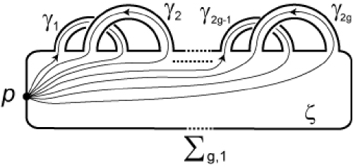
Figure 1. Cell decomposition of $\Sigma_{g,1}$

Definition 2.4.

A homology cylinder $(M,i_{+},i_{-})$ over $\Sigma_{g,1}$ consists of a compact oriented 3-manifold $M$ with two embeddings $i_{+},i_{-}:\Sigma_{g,1}\hookrightarrow\partial M$, called markings, such that:

1. $i_{+}$ is orientation-preserving and $i_{-}$ is orientation-reversing;

2. $\partial M=i_{+}(\Sigma_{g,1})\cup i_{-}(\Sigma_{g,1})$ and $i_{+}(\Sigma_{g,1})\cap i_{-}(\Sigma_{g,1})=i_{+}(\partial\Sigma_{g,1})=i_{-}(\partial\Sigma_{g,1})$;

3. $i_{+}|_{\partial\Sigma_{g,1}}=i_{-}|_{\partial\Sigma_{g,1}}$; and

4. $i_{+},i_{-}:H_{*}(\Sigma_{g,1};\mathbb{Z})\to H_{*}(M;\mathbb{Z})$ are isomorphisms.

Similarly, the definition of a rational homology cylinder is obtained by replacing (iv) with the condition that (iv’) $i_{+},i_{-}:H_{*}(\Sigma_{g,1};\mathbb{Q})\to H_{*}(M;\mathbb{Q})$ are isomorphisms.

Two homology cylinders $(M,i_{+},i_{-})$ and $(N,j_{+},j_{-})$ over $\Sigma_{g,1}$ are said to be isomorphic if there exists an orientation-preserving diffeomorphism $f:M\xrightarrow{\cong}N$ satisfying $j_{+}=f\circ i_{+}$ and $j_{-}=f\circ i_{-}$. We denote by $\mathcal{C}_{g,1}$ the set of all isomorphism classes of homology cylinders over $\Sigma_{g,1}$. By using markings, we can endow $\mathcal{C}_{g,1}$ with a monoid structure whose product is given by

$$(M,i_{+},i_{-})\cdot(N,j_{+},j_{-}):=(M\cup_{i_{-}\circ(j_{+})^{-1}}N,i_{+},j_{-})$$

for $(M,i_{+},i_{-})$, $(N,j_{+},j_{-})\in\mathcal{C}_{g,1}$. The unit of this monoid is given by

$$(M,i_{+},i_{-})=(\Sigma_{g,1}\times[0,1],\mathrm{id}\times 1,\mathrm{id}\times 0),$$

where collars of $i_{+}(\Sigma_{g,1})$ and $i_{-}(\Sigma_{g,1})$ are stretched half-way along $(\partial\Sigma_{g,1})\times[0,1]$. The monoid $\mathcal{C}_{g,1}^{\mathbb{Q}}$ of all isomorphism classes of rational homology cylinders over $\Sigma_{g,1}$ is defined similarly. For each diffeomorphism $\varphi$ of $\Sigma_{g,1}$ which fixes $\partial\Sigma_{g,1}$ pointwise, we can construct a homology cylinder as a mapping cylinder

$$(\Sigma_{g,1}\times[0,1],\mathrm{id}\times 1,\varphi\times 0)$$

of $\varphi$.

Constructing a homology cylinder from a given homologically fibered knot has an ambiguity arising from taking a minimal genus Seifert surface and fixing a pair of markings.

Proposition 2.5.

Let $R_{1}$ and $R_{2}$ be $($maybe parallel$)$ minimal genus Seifert surfaces of a homologically fibered knot of genus $g$ and let $M_{R_{1}}$ and $M_{R_{2}}$ be their sutured manifolds. For any markings $i_{\pm}$ and $j_{\pm}$ of $\partial M_{R_{1}}$ and $\partial M_{R_{2}}$, there exists another homology cylinder $N\in\mathcal{C}_{g,1}$ such that

$$(M_{R_{1}},i_{+},i_{-})\cdot N=N\cdot(M_{R_{2}},j_{+},j_{-})$$

holds as elements of $\mathcal{C}_{g,1}$.

Proof.

First we assume that $R_{1}$ and $R_{2}$ are disjoint in $E(K)$. Cut $E(K)$ along $R_{1}$ and $R_{2}$. Then we obtain two submanifolds $N$ and $N^{\prime}$ of $E(K)$, where $N$ (resp. $N^{\prime}$) may be regarded as a surface cobordism between $i_{+}(\Sigma_{g,1})$ and $j_{-}(\Sigma_{g,1})$ (resp. $j_{+}(\Sigma_{g,1})$ and $i_{-}(\Sigma_{g,1})$). We can easily check that $(N,i_{+},j_{-})$ and $(N^{\prime},j_{+},i_{-})$ are homology cylinders over $\Sigma_{g,1}$. Then the equality $M_{R_{1}}\cup_{R_{1}}N=N\cup_{R_{2}}M_{R_{2}}$ holds and it shows our claim in this case.

For the general case, we can use a theorem of Scharlemann-Thompson [30] . It says that there exists a sequence of minimal genus Seifert surfaces $R_{1}=S_{1}\rightarrow S_{2}\rightarrow\cdots\rightarrow S_{n}=R_{2}$ such that $S_{i}$ and $S_{i+1}$ are disjoint in $E(K)$ for $i=1,2,\ldots,n-1$. Using the above argument repeatedly, we have the conclusion. ∎

This proposition can be seen as a generalization of the fact that a fibered knot determines an element of the mapping class group of a surface uniquely up to conjugation.

Remark 2.6.

Differently from fibered knots, a homologically fibered knot does not necessarily have a unique minimal genus Seifert surface. Indeed, it was shown by Eisner [7] that the connected sum of two non-fibered knots has infinitely many non-isotopic minimal genus Seifert surfaces. Hence the connected sum of two non-fibered homologically fibered knots, which is again a homologically fibered knot, gives such an example. The authors do not know whether there exists a homologically fibered knot which has minimal genus Seifert surfaces whose complements are not homeomorphic.

3. Higher-order Alexander invariants

From the factorization $(\ref{eq1})$, we see that if a rationally homologically fibered knot has a non-trivial $\det(S)$-part, that is $|\det(S)|\neq 1$, then this knot is not fibered. However, this argument is useless for homologically fibered knots, since $|\det(S)|=1$. In this section, we give a generalization of the factorization $(\ref{eq1})$ by using the framework of higher-order Alexander invariants originally due to Cochran [4] and Harvey [18] together with their interpretations as Reidemeister torsions given by Friedl [8]. We will see later that this generalized factorization works well for homologically fibered knots.

We begin by summarizing our notation. For a matrix $A$ with entries in a group ring $\mathbb{Z}G$ (or its quotient field) for a group $G$, we denote by $\overline{A}$ the matrix obtained from $A$ by applying the involution induced from $(x\mapsto x^{-1},\ x\in G)$ to each entry. For a module $M$, we write $M^{n}$ for the module of column vectors with $n$ entries. For a finite cell complex $X$, we denote by $\widetilde{X}$ its universal covering. We take a base point $p$ of $X$ and a lift $\widetilde{p}$ of $p$ as a base point of $\widetilde{X}$. $\pi:=\pi_{1}(X,p)$ acts on $\widetilde{X}$ from the right through its deck transformation group, so that the lift of a loop $l\in\pi$ starting from $\widetilde{p}$ reaches $\widetilde{p}\,l^{-1}$. Then the cellular chain complex $C_{\ast}(\widetilde{X})$ of $\widetilde{X}$ becomes a right $\mathbb{Z}\pi$-module. For each left $\mathbb{Z}\pi$-algebra $\mathcal{R}$, the twisted chain complex $C_{\ast}(X;\mathcal{R})$ is given by the tensor product of the right $\mathbb{Z}\pi$-module $C_{\ast}(\widetilde{X})$ and the left $\mathbb{Z}\pi$-module $\mathcal{R}$, so that $C_{\ast}(X;\mathcal{R})$ and $H_{\ast}(X;\mathcal{R})$ are right $\mathcal{R}$-modules.

In the definition of higher-order Alexander invariants, PTFA groups play important roles, where a group $\Gamma$ is said to be poly-torsion-free abelian $($PTFA$)$ if it has a sequence

$$\Gamma=\Gamma_{0}\triangleright\Gamma_{1}\triangleright\cdots\triangleright\Gamma_{n}=\{1\}$$

whose successive quotients $\Gamma_{i}/\Gamma_{i+1}$ $(i\geq 0)$ are all torsion-free abelian. An advantage of using PTFA groups is that the group ring $\mathbb{Z}\Gamma$ (or $\mathbb{Q}\Gamma$) of $\Gamma$ is known to be an Ore domain so that it can be embed into the field (skew field in general)

$$\mathcal{K}_{\Gamma}:=\mathbb{Z}\Gamma(\mathbb{Z}\Gamma-\{0\})^{-1}=\mathbb{Q}\Gamma(\mathbb{Q}\Gamma-\{0\})^{-1}$$

called the right field of fractions. We refer to [4] and [28] for generalities of PTFA groups and localizations of their group rings. A typical example of PTFA groups is $\mathbb{Z}^{n}$, where $\mathcal{K}_{\mathbb{Z}^{n}}$ is isomorphic to the field of rational functions with $n$ variables.

For a rationally homologically fibered knot $K$, we take a non-trivial homomorphism $\rho:G(K)\to\Gamma$ to a PTFA group $\Gamma$, where $G(K)$ denotes the knot group $\pi_{1}(E(K))$. We can regard $\mathcal{K}_{\Gamma}$ as a local coefficient system on $E(K)$ through $\rho$. Using arguments in Cochran-Orr-Teichner [5, Section 2] and Cochran [4, Section 3], we have:

Lemma 3.1.

For any non-trivial homomorphism $\rho:G(K)\to\Gamma$ to a PTFA group $\Gamma$, we have $H_{\ast}(E(K);\mathcal{K}_{\Gamma})=0$.

By this lemma, we can define the Reidemeister torsion

$$\tau_{\rho}(E(K)):=\tau(C_{\ast}(E(K);\mathcal{K}_{\Gamma}))\in K_{1}(\mathcal{K}_{\Gamma})/\pm\rho(G(K))$$

for the acyclic complex $C_{\ast}(E(K);\mathcal{K}_{\Gamma})$. We refer to Milnor [26] for generalities of torsions. By higher-order Alexander invariants for $K$, we here mean this torsion $\tau_{\rho}(E(K))$.

We now describe a factorization of $\tau_{\rho}(E(K))$ generalizing (1.1). For that we use two kinds of invariants for rational homology cylinders from [29] and [14]. Let $(M_{R},i_{+},i_{-})\in\mathcal{C}_{g,1}^{\mathbb{Q}}$ be the rational homology cylinder obtained as the sutured manifold for a minimal genus Seifert surface $R$ of $K$. We use the same notation $\rho:\pi_{1}(M_{R})\to\Gamma$ for the composition $\pi_{1}(M_{R})\to G(K)\xrightarrow{\rho}\Gamma$. By applying Cochran-Orr-Teichner [5, Proposition 2.10], we have:

Lemma 3.2.

$i_{+},i_{-}:H_{\ast}(\Sigma_{g,1},p;i_{\pm}^{\ast}\mathcal{K}_{\Gamma})\to H_{\ast}(M_{R},p;\mathcal{K}_{\Gamma})$ are isomorphisms as right $\mathcal{K}_{\Gamma}$-vector spaces. Equivalently, $H_{\ast}(M_{R},i_{\pm}(\Sigma_{g,1});\mathcal{K}_{\Gamma})=0$.

This lemma provides the following two kinds of invariants for $M_{R}$.

The Magnus matrix  Let $X\subset\Sigma_{g,1}$ be the union of $2g$ loops $\gamma_{1},\ldots,\gamma_{2g}$ (see Figure 1). $X$ is a deformation retract of $\Sigma_{g,1}$ relative to $p$. Therefore, for $\pm\in\{+,-\}$, we have

$$H_{1}(\Sigma_{g,1},p;i_{\pm}^{\ast}\mathcal{K}_{\Gamma})\cong H_{1}(X,p;i_{\pm}^{\ast}\mathcal{K}_{\Gamma})=C_{1}(\widetilde{X})\otimes_{\pi_{1}(\Sigma_{g,1})}i_{\pm}^{\ast}\mathcal{K}_{\Gamma}\cong\mathcal{K}_{\Gamma}^{2g}$$

with a basis

$$\{\widetilde{\gamma}_{1}\otimes 1,\ldots,\widetilde{\gamma}_{2g}\otimes 1\}\subset C_{1}(\widetilde{X})\otimes_{\pi_{1}(\Sigma_{g,1})}i_{\pm}^{\ast}\mathcal{K}_{\Gamma}$$

as a right $\mathcal{K}_{\Gamma}$-vector space. Here we fix a lift $\widetilde{p}$ of $p$ as a base point of $\widetilde{X}$, and denote by $\widetilde{\gamma}_{i}$ the lift of the oriented loop $\gamma_{i}$ starting from $\widetilde{p}$.

Definition 3.3.

For $M_{R}=(M_{R},i_{+},i_{-})\in\mathcal{C}_{g,1}^{\mathbb{Q}}$, the Magnus matrix

$$r_{\rho}(M_{R})\in GL(2g,\mathcal{K}_{\Gamma})$$

of $M_{R}$ is defined as the representation matrix of the right $\mathcal{K}_{\Gamma}$-isomorphism

$$\mathcal{K}_{\Gamma}^{2g}\cong H_{1}(\Sigma_{g,1},p;i_{-}^{\ast}\mathcal{K}_{\Gamma})\xrightarrow[i_{-}]{\cong}H_{1}(M_{R},p;\mathcal{K}_{\Gamma})\xrightarrow[i_{+}^{-1}]{\cong}H_{1}(\Sigma_{g,1},p;i_{+}^{\ast}\mathcal{K}_{\Gamma})\cong\mathcal{K}_{\Gamma}^{2g},$$

where the first and the last isomorphisms use the bases mentioned above.

The matrix $r_{\rho}(M_{R})$ can be interpreted as a monodromy of $M_{R}$ from a view point of the twisted homology with coefficients in $\mathcal{K}_{\Gamma}$.

$\Gamma$-torsion  Since the relative complex $C_{\ast}(M_{R},i_{+}(\Sigma_{g,1});\mathcal{K}_{\Gamma})$ obtained from any cell decomposition of $(M_{R},i_{+}(\Sigma_{g,1}))$ is acyclic by Lemma 3.2, we can define the following:

Definition 3.4.

For $M_{R}=(M_{R},i_{+},i_{-})\in\mathcal{C}_{g,1}^{\mathbb{Q}}$, the $\Gamma$-torsion $\tau_{\rho}^{+}(M_{R})$ of $M_{R}$ is defined by

$$\tau_{\rho}^{+}(M_{R}):=\tau(C_{\ast}(M_{R},i_{+}(\Sigma_{g,1});\mathcal{K}_{\Gamma}))\in K_{1}(\mathcal{K}_{\Gamma})/\pm\rho(\pi_{1}(M_{R})).$$

A method for computing $r_{\rho}(M_{R})$ and $\tau_{\rho}^{+}(M_{R})$ is given in [14, Section 4], which is based on Kirk-Livingston-Wang’s method [22] for invariants of string links, and we now recall it briefly. An admissible presentation of $\pi_{1}(M_{R})$ is defined to be the one of the form

(3.1) $$\langle i_{-}(\gamma_{1}),\ldots,i_{-}(\gamma_{2g}),z_{1},\ldots,z_{l},i_{+}(\gamma_{1}),\ldots,i_{+}(\gamma_{2g})\mid r_{1},\ldots,r_{2g+l}\rangle$$

for some integer $l$. That is, it is a finite presentation with deficiency $2g$ whose generating set contains $i_{-}(\gamma_{1}),\ldots,i_{-}(\gamma_{2g}),i_{+}(\gamma_{1}),\ldots,i_{+}(\gamma_{2g})$ and is ordered as above. Such a presentation always exists (see [14, Section 4]). For any admissible presentation, define $2g\times(2g+l)$, $l\times(2g+l)$ and $2g\times(2g+l)$ matrices $A,B,C$ over $\mathbb{Z}\Gamma$ by

$$A=\overline{\sideset{{}^{\rho}\!}{}{\mathop{\left({\displaystyle\frac{\partial r_{j}}{\partial i_{-}(\gamma_{i})}}\right)}\nolimits}}_{\begin{subarray}{c}{}1\leq i\leq 2g\\ 1\leq j\leq 2g+l\end{subarray}},\ \ B=\overline{\sideset{{}^{\rho}\!}{}{\mathop{\left({\displaystyle\frac{\partial r_{j}}{\partial z_{i}}}\right)}\nolimits}}_{\begin{subarray}{c}{}1\leq i\leq l\\ 1\leq j\leq 2g+l\end{subarray}},\ \ C=\overline{\sideset{{}^{\rho}\!}{}{\mathop{\left({\displaystyle\frac{\partial r_{j}}{\partial i_{+}(\gamma_{i})}}\right)}\nolimits}}_{\begin{subarray}{c}{}1\leq i\leq 2g\\ 1\leq j\leq 2g+l\end{subarray}}.$$

Proposition 3.5 ([14, Proposition 4.1]).

As matrices with entries in $\mathcal{K}_{\Gamma}$, we have:

• The square matrix $\begin{pmatrix}A\\ B\end{pmatrix}$ is invertible and $\tau_{\rho}^{+}(M_{R})=\begin{pmatrix}A\\ B\end{pmatrix}$; and

• $r_{\rho}(M_{R})=-C\begin{pmatrix}A\\ B\end{pmatrix}^{-1}\!\begin{pmatrix}I_{2g}\\ 0_{(l,2g)}\end{pmatrix}$.

Remark 3.6.

We see from Strebel [31] that for a PTFA group $\Gamma$, every matrix with entries in $\mathbb{Z}\Gamma$ sent to an invertible matrix over $\mathbb{Q}$ by the augmentation map $\mathbb{Z}\Gamma\to\mathbb{Z}$ is invertible over $\mathcal{K}_{\Gamma}$. The first assertion of (1) follows from this fact. Indeed, $\begin{pmatrix}A\\ B\end{pmatrix}$ is sent to a representation matrix of $H_{1}(M_{R};\mathbb{Q})/i_{+}(H_{1}(\Sigma_{g,1};\mathbb{Q}))=0$ by the augmentation map, which is invertible over $\mathbb{Q}$.

Remark 3.7.

If $K$ is fibered, the complementary sutured manifold for the unique minimal genus Seifert surface is a product sutured manifold, so that $\Gamma$-torsion is trivial for any $\Gamma$. Therefore we can use $\Gamma$-torsion as fibering obstructions of homologically fibered knots. Note that we can also use the Magnus matrix (see [14, Theorem 4.1] and Section 6).

By using the above invariants, the factorization formula for $\tau_{\rho}(E(K))$ is given as follows, where the statement is simpler than that in [14] because we are now considering the knot cases only.

Theorem 3.8.

Let $K$ be a rationally homologically fibered knot of genus $g$ and let $R$ be a minimal genus Seifert surface of $K$. For any non-trivial homomorphism $\rho:G(K)\to\Gamma$ to a PTFA group $\Gamma$, a loop $\mu$ representing the meridian of $K$ satisfies $\rho(\mu)\neq 1\in\Gamma\subset\mathcal{K}_{\Gamma}$ and we have a factorization

(3.2) $$\tau_{\rho}(E(K))=\frac{\tau_{\rho}^{+}(M_{R})\cdot(I_{2g}-\rho(\mu)r_{\rho}(M_{R}))}{1-\rho(\mu)}\quad\in K_{1}(\mathcal{K}_{\Gamma})/\pm\rho(G(K))$$

of the torsion $\tau_{\rho}(E(K))$.

Proof.

First, by passing to the image if necessary, we may suppose that $\rho$ is onto. This is justified by the facts that any subgroup $\Gamma^{\prime}$ of a PTFA group $\Gamma$ is again PTFA and that the torsion is invariant under the field extension $\mathcal{K}_{\Gamma^{\prime}}\hookrightarrow\mathcal{K}_{\Gamma}$.

By the definition of PTFA groups, we see that there exists a surjective homomorphism $\Gamma\to\mathbb{Z}$. Then the composite $G(K)\xrightarrow{\rho}\Gamma\to\mathbb{Z}$ is also surjective and it coincides with the abelianization map of $G(K)$ up to sign. Hence $\rho(\mu)\neq 1\in\Gamma$.

The rest of the proof is almost identical to the argument in [14, Section 5] (see also the argument of Friedl [8, Section 6]). For convenience, we repeat it here in a simplified form.

Given an admissible presentation of $\pi_{1}(M_{R})$ as in (3.1), we denote it briefly by

$$\pi_{1}(M_{R})\cong\langle i_{-}(\overrightarrow{\gamma}),\overrightarrow{z},i_{+}(\overrightarrow{\gamma})\mid\overrightarrow{r}\rangle.$$

A usual computation gives

$$G(K)\cong\langle i_{-}(\overrightarrow{\gamma}),\overrightarrow{z},i_{+}(\overrightarrow{\gamma}),\mu\mid\overrightarrow{r},i_{-}(\overrightarrow{\gamma})\,\mu\,i_{+}(\overrightarrow{\gamma})^{-1}\mu^{-1}\rangle.$$

From this presentation, we construct a 2-complex $X(K)$ consisting of one 0-cell, one 1-cell for each generator and one 2-cell for each relation with an attaching map according to the word. We can check that $E(K)$ and $X(K)$ are simple homotopy equivalent (see [14, Lemma 5.1]).

The $\mathcal{K}_{\Gamma}$-rank of $C_{i}(X(K);\mathcal{K}_{\Gamma})$ and the $\mathbb{Z}$-rank $C_{i}(X(K))$ are the same and their degree $0,1,2$ parts are given by $1,4g+l+1,4g+l$. The map $\partial_{2}:C_{2}(X(K);\mathcal{K}_{\Gamma})\cong\mathcal{K}_{\Gamma}^{4g+l}\to C_{1}(X(K);\mathcal{K}_{\Gamma})\cong\mathcal{K}_{\Gamma}^{4g+l+1}$ is represented by the matrix

$$D_{2}:=\begin{pmatrix}A&I_{2g}\\ B&0_{(l,2g)}\\ C&-\rho(\mu)^{-1}I_{2g}\\ 0_{(1,2g+l)}&\ast\ \ast\ \cdots\ \ast\end{pmatrix}.$$

Consider the matrix $D_{2}^{\mu}$ obtained from $D_{2}$ by deleting the last row. By fundamental transformations of matrices, we have

$$D_{2}^{\mu} =\begin{pmatrix}A\ &I_{2g}\\ B\ &0_{(l,2g)}\\ C\ &-\rho(\mu)^{-1}I_{2g}\end{pmatrix}\to\begin{pmatrix}A+\rho(\mu)C&0_{2g}\\ B&0_{(l,2g)}\\ C&-\rho(\mu)^{-1}I_{2g}\end{pmatrix}$$

$$\to\begin{pmatrix}A+\rho(\mu)C&0_{2g}\\ B&0_{(l,2g)}\\ 0_{(2g,2g+l)}&-\rho(\mu)^{-1}I_{2g}\end{pmatrix}=:D$$

Here the above matrices are with entries in $\mathbb{Z}\Gamma$ and we apply the augmentation map $\mathbb{Z}\Gamma\to\mathbb{Z}$ to $D$. Then we have a matrix representing $\partial_{2}:C_{2}(X(K))\to C_{1}(X(K))/\langle\mu\rangle$, which can be easily seen to be invertible over $\mathbb{Q}$. Hence $D$ (and also $D_{2}^{\mu}$) is invertible over $\mathcal{K}_{\Gamma}$ as mentioned in Remark 3.6.

Now we compute $\tau_{\rho}(E(K))=\tau(C_{\ast}(X(K);\mathcal{K}_{\Gamma}))$. By the cell structure of $X(K)$,

$$\tau_{\rho}(E(K))=D_{2}^{\mu}\cdot(1-\rho(\mu)^{-1})^{-1}$$

holds. Then as elements in $K_{1}(\mathcal{K}_{\Gamma})/\pm\rho(G(K))$, we have

$$D_{2}^{\mu} =D=\begin{pmatrix}A+\rho(\mu)C\\ B\end{pmatrix}=\begin{pmatrix}I_{2g}-\rho(\mu)r_{\rho}(M_{R})&\ -\rho(\mu)Z\\ 0_{(l,2g)}&\ I_{l}\end{pmatrix}\begin{pmatrix}A\\ B\end{pmatrix}$$

$$=(I_{2g}-\rho(\mu)r_{\rho}(M_{R}))\begin{pmatrix}A\\ B\end{pmatrix},$$

where we used

$$\begin{pmatrix}A+\rho(\mu)C\\ B\end{pmatrix}=\begin{pmatrix}A\\ B\end{pmatrix}-\rho(\mu)\begin{pmatrix}r_{\rho}(M_{R})\quad Z\\ 0_{(l,2g+l)}\end{pmatrix}\begin{pmatrix}A\\ B\end{pmatrix}$$

at the third equality and $Z$ is defined by the formula $(r_{\rho}(M_{R})\quad Z)=-C\begin{pmatrix}A\\ B\end{pmatrix}^{-1}$ (see Proposition 3.5 (2)). This completes the proof. ∎

When we take the abelianization map $\rho_{1}:G(K)\to\langle t\rangle\subset\mathbb{Q}(t)$ as $\rho$, the formula (1.1) is recovered.

Remark 3.9.

Factorizations of (higher-order) Alexander invariants into some torsions and “monodromy” information appear in various contexts such as Morse-Novikov theory and the theory of string links. For example, see Hutchings-Lee [19, 20], Goda-Matsuda-Pajitnov [13], Kitayama [23] and Kirk-Livingston-Wang [22]. It would be interesting to compare these factorization formulas in an appropriate situation.

4. A sample calculation

Although all the ingredients in the formula $(\ref{eq2})$ are determined by information on fundamental groups, it is difficult to compute them explicitly because of the non-commutativity of $\mathcal{K}_{\Gamma}$ except in some special cases including the following.

Let $K$ be a homologically fibered knot with a minimal genus Seifert surface $R$ and let $M_{R}$ be the sutured manifold for $R$. Consider the group extension

(4.1) $$1\longrightarrow G(K)^{\prime}/G(K)^{\prime\prime}\longrightarrow D_{2}(K)\longrightarrow G(K)/G(K)^{\prime}=H_{1}(E(K))\cong\mathbb{Z}\longrightarrow 1$$

relating to the metabelian quotient $D_{2}(K):=G(K)/G(K)^{\prime\prime}$ of $G(K)$. We have

$$G(K)^{\prime}/G(K)^{\prime\prime}\cong H_{1}(R)\cong H_{1}(M_{R})$$

since it coincides with the first homology of the infinite cyclic covering of $E(K)$, which can be seen as the product (as homology cylinders) of infinitely many copies of $M_{R}$. Let $\rho_{2}$ be the natural projection

$$\rho_{2}:G(K)\longrightarrow D_{2}(K).$$

It is known that $D_{2}(K)$ is PTFA (see Strebel [31]), so that $\mathcal{K}_{D_{2}(K)}$ is defined. Then, it follows from the Proposition 3.5 that $\tau_{\rho_{2}}^{+}(M_{R})$ and $r_{\rho_{2}}(M_{R})$ can be computed by calculations on the commutative subfield $\mathcal{K}_{H_{1}(M_{R})}$ of $\mathcal{K}_{D_{2}(K)}$, and therefore we can carry it out.

Let us see an example of calculations of our invariants. Let $K$ be the knot obtained as the boundary of the Seifert surface $R$ illustrated in Figure 2. We can easily compute that $\Delta_{K}(t)=1-2t+3t^{2}-2t^{3}+t^{4}$ and the genus of $R$ is $2$. Hence $K$ is a homologically fibered knot and $R$ is of minimal genus. The graph $G$ in right hand side of Figure 2 is obtained from $R$ by a deformation retract. Thus $\pi_{1}(M_{R})\cong\pi_{1}(S^{3}-\overset{\circ}{N}(G))$. Then $\pi_{1}(M_{R})$ has a presentation:

$${\small\left\langle\begin{array}[]{c|l}z_{1},z_{2},\ldots,z_{10}&\ \begin{array}[]{ll}z_{1}z_{5}z_{6}^{-1},\,z_{2}z_{3}z_{4}z_{1},\,z_{3}z_{9}^{-1}z_{5}^{-1},\,z_{7}z_{4}z_{8}^{-1},\\ z_{8}z_{10}z_{6},\,z_{2}z_{5}z_{7}^{-1}z_{5}^{-1},\,z_{9}z_{4}z_{10}^{-1}z_{4}^{-1}\end{array}\end{array}\right\rangle.}$$

We can drop the last relation $z_{9}z_{4}z_{10}^{-1}z_{4}^{-1}$ because it is derived from the others.

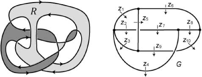
Figure 2.

We take a spine of $R$ as in Figure 3, by which we can fix an identification of $\Sigma_{g,1}$ and $R$.

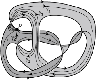
Figure 3.

A direct computation shows that

$$i_{-}(\gamma_{1}) =z_{5}z_{1}, i_{-}(\gamma_{2}) =z_{2}^{-1}, i_{-}(\gamma_{3}) =z_{5}z_{7}^{-1}z_{8}^{-1}z_{4}^{-1}, i_{-}(\gamma_{4}) =z_{4}^{-1},$$

$$i_{+}(\gamma_{1}) =z_{5}, i_{+}(\gamma_{2}) =z_{6}z_{9}, i_{+}(\gamma_{3}) =z_{6}z_{5}^{-1}z_{3}z_{5}z_{7}^{-1}z_{4}^{-1}z_{6}^{-1}, i_{+}(\gamma_{4}) =z_{6}z_{7}z_{6}^{-1}.$$

Here the darker color in $R$ is the $+$-side. Then, we obtain an admissible presentation of $\pi_{1}(M_{R})$:

Generators	$i_{-}(\gamma_{1}),\ldots,i_{-}(\gamma_{4}),\,z_{1},\ldots,z_{10},\,i_{+}(\gamma_{1}),\ldots,i_{+}(\gamma_{4})$
Relations	$z_{1}z_{5}z_{6}^{-1},\,z_{2}z_{3}z_{4}z_{1},\,z_{3}z_{9}^{-1}z_{5}^{-1},\,z_{7}z_{4}z_{8}^{-1},\,z_{8}z_{10}z_{6},\,z_{2}z_{5}z_{7}^{-1}z_{5}^{-1},$
	$i_{-}(\gamma_{1})z_{1}^{-1}z_{5}^{-1},\,i_{-}(\gamma_{2})z_{2},\,i_{-}(\gamma_{3})z_{4}z_{8}z_{7}z_{5}^{-1},\,i_{-}(\gamma_{4})z_{4},$
	$i_{+}(\gamma_{1})z_{5}^{-1},\,i_{+}(\gamma_{2})z_{9}^{-1}z_{6}^{-1},\,i_{+}(\gamma_{3})z_{6}z_{4}z_{7}z_{5}^{-1}z_{3}^{-1}z_{5}z_{6}^{-1},\,i_{+}(\gamma_{4})z_{6}z_{7}^{-1}z_{6}^{-1}$

By sliding the edges $v_{1}$ and $v_{2}$ of $G$ as in Figure 4, we obtain a graph whose complement is a genus 4 handlebody. This means that the complement of $G$ (and hence $M_{R}$) is homeomorphic to a genus 4 handlebody.

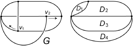
Figure 4.

Let $D_{1},\ldots,D_{4}$ be the meridian disks of the handlebody as illustrated in the figure. Put $x_{1}:=z_{1}^{-1}$, $x_{2}=z_{6}^{-1}$, $x_{3}:=(z_{6}z_{7})^{-1}$ and $x_{4}:=z_{4}$, where $x_{i}$ is a loop intersecting $D_{i}$ transversely in one point from the above to the down side in Figure 4 and is disjoint from $D_{j}\,(i\neq j)$. By using them, we have the following simplified admissible presentation of $\pi_{1}(M_{R})$:

Generators	$i_{-}(\gamma_{1}),\ldots,i_{-}(\gamma_{4}),\,x_{1},x_{2},x_{3},x_{4},\,i_{+}(\gamma_{1}),\ldots,i_{+}(\gamma_{4})$
Relations	$i_{-}(\gamma_{1})x_{1}x_{2}x_{1}^{-1}$,   $i_{-}(\gamma_{2})x_{1}x_{3}^{-1}x_{2}x_{1}^{-1}$,   $i_{-}(\gamma_{3})x_{4}x_{2}x_{3}^{-1}x_{4}x_{2}x_{3}^{-1}x_{2}x_{1}^{-1}$,
	$i_{-}(\gamma_{4})x_{4}$,  $i_{+}(\gamma_{1})x_{2}x_{1}^{-1},$   $i_{+}(\gamma_{2})x_{4}x_{3}^{-1}x_{2}$,
	$i_{+}(\gamma_{3})x_{2}^{-1}x_{4}x_{2}x_{3}^{-1}x_{2}x_{1}^{-1}x_{4}x_{3}^{-1}x_{2}$,  $i_{+}(\gamma_{4})x_{2}^{-1}x_{3}$

We write $r_{1},\ldots,r_{8}$ for these relations in order. Recall that $\mathcal{K}_{H_{1}(M_{R})}$ is isomorphic to the field of rational functions with variables $x_{1},\ldots,x_{4}$, where we use the same notation for the image of $x_{i}$ by the abelianization map $\pi_{1}(M_{R})\to H_{1}(M_{R})$. Then we have

$$\begin{pmatrix}A\\ B\\ C\end{pmatrix}=\begin{pmatrix}I_{4}&0_{4}\\ G_{1}&G_{2}\\ 0_{4}&I_{4}\end{pmatrix},$$

where $G_{1}=\begin{pmatrix}g_{11}&g_{12}&g_{13}&g_{14}\\ g_{21}&g_{22}&g_{23}&g_{24}\\ g_{31}&g_{32}&g_{33}&g_{34}\\ g_{41}&g_{42}&g_{43}&g_{44}\end{pmatrix}$ and $G_{2}=\begin{pmatrix}g_{15}&g_{16}&g_{17}&g_{18}\\ g_{25}&g_{26}&g_{27}&g_{28}\\ g_{35}&g_{36}&g_{37}&g_{38}\\ g_{45}&g_{46}&g_{47}&g_{48}\end{pmatrix}$ with $g_{ij}=\rho\left(\overline{\displaystyle\frac{\partial r_{j}}{\partial x_{i}}}\right)$. Thus

$$\tau_{\rho_{2}}^{+}(M_{R})=\begin{pmatrix}A\\ B\end{pmatrix}=\begin{pmatrix}I_{4}&0_{4}\\ G_{1}&G_{2}\end{pmatrix}.$$

As a torsion, it is equivalent to $G_{2}$, where

$$g_{15} =-1, \quad g_{16} =0, \quad g_{18} =0,$$

$$g_{25} =x_{1}^{-1}x_{2}, \quad g_{26} =x_{2}, \quad g_{28} =-x_{3},$$

$$g_{35} =0, \quad g_{36} =-x_{2}, \quad g_{38} =x_{3},$$

$$g_{45} =0, \quad g_{46} =x_{2}x_{3}^{-1}x_{4}, \quad g_{48} =0,$$

$$g_{17} =-x_{2}x_{3}^{-1}x_{4},\qquad g_{27}=x_{2}+x_{1}^{-1}x_{2}^{2}x_{3}^{-1}x_{4}+x_{1}^{-1}x_{2}^{3}x_{3}^{-2}x_{4}-x_{1}^{-1}x_{2}^{3}x_{3}^{-2}x_{4}^{2},$$

$$g_{37} =-x_{2}-x_{1}^{-1}x_{2}^{2}x_{3}^{-1}x_{4},\qquad g_{47}=x_{2}x_{3}^{-1}x_{4}+x_{1}^{-1}x_{2}^{3}x_{3}^{-2}x_{4}^{2}.$$

Then we have

$$\det(\tau_{\rho_{2}}^{+}(M_{R}))=\det(G_{2})=-\frac{x_{2}^{3}x_{4}^{2}}{x_{1}x_{3}^{2}}(x_{2}-x_{3}-x_{2}x_{4}).$$

The Magnus matrix $r_{\rho_{2}}(M_{R})$ can be computed by the formula in Proposition 3.5 (2). However we omit it here.

Remark 4.1.

From an admissible presentation, we can use the Mathematica program given in Section 7 for calculations of $\tau_{\rho_{2}}^{+}(M_{R})$ and $r_{\rho_{2}}(M_{R})$. Note that the program uses $\{i_{+}(\gamma_{1}),i_{+}(\gamma_{2}),\ldots,i_{+}(\gamma_{2g})\}$ as a basis of $H_{1}(M_{R})$. In the above example,

$$x_{1}=\gamma_{2}^{-2}\gamma_{3},\quad x_{2}=\gamma_{1}^{-1}\gamma_{2}^{-2}\gamma_{3},\quad x_{3}=\gamma_{1}^{-1}\gamma_{2}^{-2}\gamma_{3}\gamma_{4}^{-1},\quad x_{4}=\gamma_{2}^{-1}\gamma_{4}^{-1},$$

where $\gamma_{j}$ denotes $i_{+}(\gamma_{j})$, and we have $\det(\tau_{\rho_{2}}^{+}(M_{R}))=\displaystyle\frac{\gamma_{3}}{\gamma_{1}^{2}\gamma_{2}^{5}\gamma_{4}}(1+\gamma_{2}-\gamma_{2}\gamma_{4})$.

5. Homologically fibered knots with 12-crossings

It is known that all homologically fibered knots are fibered among prime knots with at most 11-crossings. On the other hand, Friedl-Kim [10] showed that there are 13 non-fibered homologically fibered knots with 12-crossings by using the twisted Alexander invariant. See Figure 5 and Table 1. In this section, we list admissible presentations and the torsion $\tau^{+}_{\rho_{2}}$ for sutured manifolds associated with minimal genus Seifert surfaces illustrated in Figure $\ref{fig:0210SG},\ldots,\ref{fig:0815SG}$. As a by-product, we observe that $\tau^{+}_{\rho_{2}}$ can also detect the non-fiberedness of all these knots. In the forthcoming paper [15], we will obtain the same result by using Johnson homomorphisms as a fibering obstruction.

It is easy to see that the complements of the Seifert surfaces for knots 0210, 0214, 0382 and 0394 are handlebodies. (In [3], a non-alternating prime knot with 12-crossings is denoted by $12n_{-}P$. We refer only the number $P$ in this section.) Hence, we take free generators corresponding to disks $z_{i}$ in each figure, which run from the upside to the downside of the diagrams. As for the other knots, we have the admissible presentations by the same method as in Section 4.

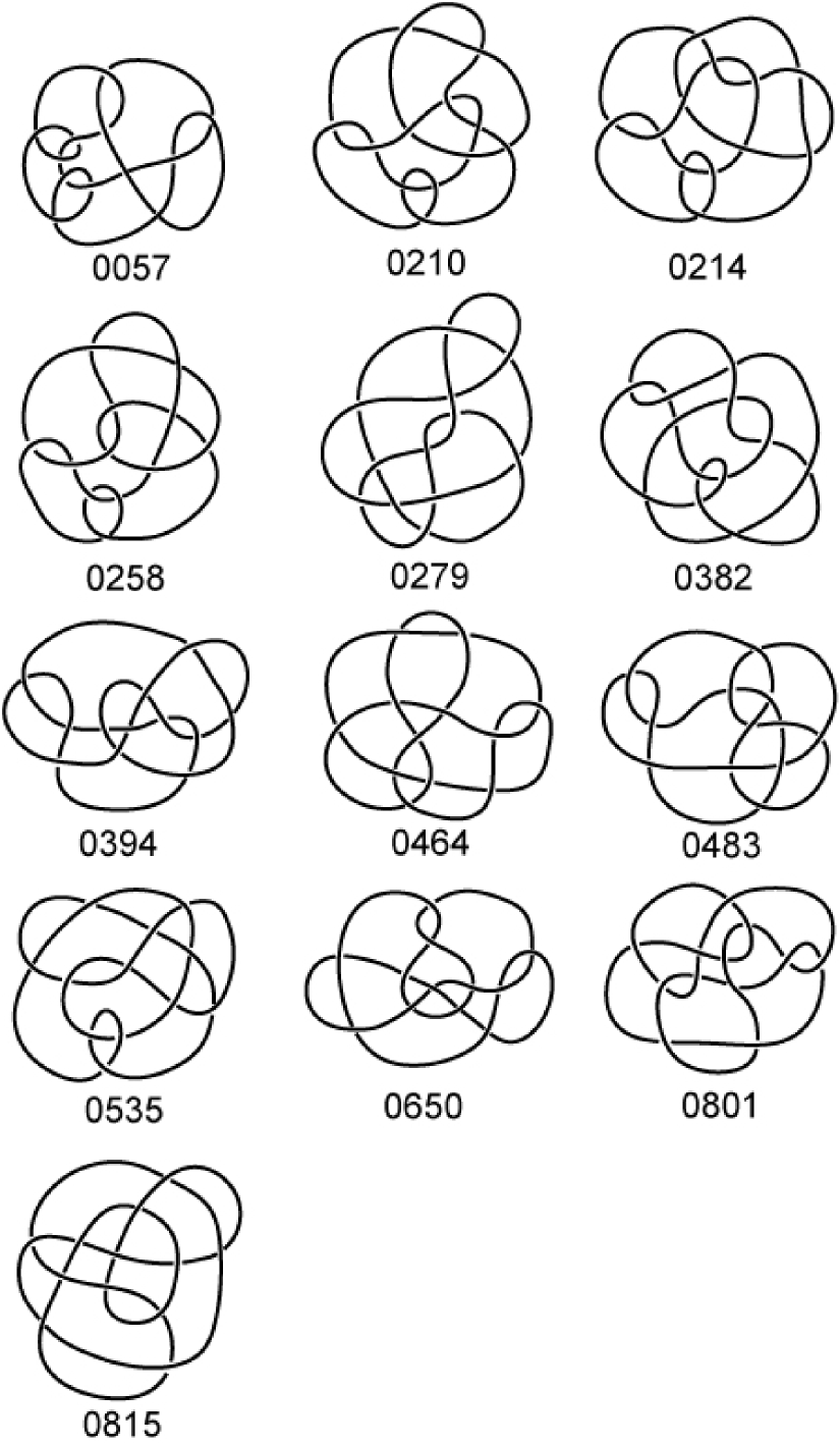
Figure 5. 12-crossings non-fibered homologically fibered knots

Knot	Genus	Alexander polynomial
0057	2	$1-2t+3t^{2}-2t^{3}+t^{4}$
0210, 0214	3	$1-t-t^{2}+3t^{3}-t^{4}-t^{5}+t^{6}$
0258, 0464, 0483	2	$1-4t+5t^{2}-4t^{3}+t^{4}$
0279, 0394	2	$1-6t+11t^{2}-6t^{3}+t^{4}$
0382, 0801	2	$1-5t+7t^{2}-5t^{3}+t^{4}$
0535	2	$1-7t+11t^{2}-7t^{3}+t^{4}$
0650	2	$1-4t+7t^{2}-4t^{4}+t^{4}$
0815	2	$1-2t+t^{2}-2t^{3}+t^{4}$

Table 1. Non-fibered homologically fibered knots with 12-crossings

The following are admissible presentations and the determinant of the torsion $\tau^{+}_{\rho_{2}}(M_{R})$, where we use $\{i_{+}(\gamma_{1}),i_{+}(\gamma_{2}),\ldots,i_{+}(\gamma_{2g})\}$ as a basis of $H_{1}(M_{R})$ and denote $i_{+}(\gamma_{j})$ by $\gamma_{j}$ for simplicity. Note that the example in Section 4 is about the knot 0057, and we omit it here.

0210
Generators	$i_{-}(\gamma_{1}),\ldots,i_{-}(\gamma_{6}),\,z_{1},\ldots z_{6},\,i_{+}(\gamma_{1}),\ldots,i_{+}(\gamma_{6})$
Relations	$i_{-}(\gamma_{1})z_{3}^{-1}z_{4},\,i_{-}(\gamma_{2})z_{3}^{-2}z_{2},\,i_{-}(\gamma_{3})z_{5}^{-1}z_{3}^{-1}z_{2},\,i_{-}(\gamma_{4})z_{2}^{-1}z_{1}z_{6}^{-1}z_{5}z_{6}^{-1}z_{5},\,$
	$i_{-}(\gamma_{5})z_{5}^{-1}z_{6}z_{5}^{-1}z_{1}z_{6}^{-1}z_{5}z_{6}^{-1}z_{5},\,i_{-}(\gamma_{6})z_{5}^{-1}z_{6}z_{5}^{-1}z_{1}z_{3}^{-1}z_{5}z_{6}^{-1}z_{5},\,$
	$i_{+}(\gamma_{1})z_{4},\,i_{+}(\gamma_{2})z_{4}z_{3}^{-1}z_{2}z_{3}^{-1},\,i_{+}(\gamma_{3})z_{6}^{-1}z_{2}z_{3}^{-1},\,i_{+}(\gamma_{4})z_{5}z_{2}^{-1}z_{1}z_{6}^{-1}z_{5},\,$
	$i_{+}(\gamma_{5})z_{5}^{-1}z_{6}z_{2}^{-1}z_{1}z_{6}^{-1}z_{5},\,i_{+}(\gamma_{6})z_{5}^{-1}z_{6}z_{3}^{-1}z_{5}z_{6}^{-1}z_{5}\,$
Torsion $\tau^{+}_{\rho_{2}}$	$\displaystyle{-\frac{\gamma_{1}^{5}\gamma_{3}^{3}\gamma_{5}^{4}\gamma_{6}^{7}}{\gamma_{2}^{6}\gamma_{4}^{6}}+\frac{\gamma_{1}^{6}\gamma_{3}^{4}\gamma_{5}^{4}\gamma_{6}^{7}}{\gamma_{2}^{7}\gamma_{4}^{6}}-\frac{\gamma_{1}^{6}\gamma_{3}^{4}\gamma_{5}^{4}\gamma_{6}^{8}}{\gamma_{2}^{7}\gamma_{4}^{6}}}$

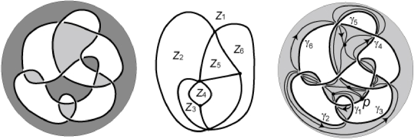
Figure 6. 0210

0214
Generators	$i_{-}(\gamma_{1}),\ldots,i_{-}(\gamma_{6}),\,z_{1},\ldots z_{6},\,i_{+}(\gamma_{1}),\ldots,i_{+}(\gamma_{6})$
Relations	$i_{-}(\gamma_{1})z_{2}z_{3}^{-1}z_{2}^{-1},\,i_{-}(\gamma_{2})z_{2}z_{1}^{-1}z_{2},\,i_{-}(\gamma_{3})z_{5}^{-1}z_{1}^{-1}z_{2},\,$
	$i_{-}(\gamma_{4})z_{6}^{-1}z_{1}z_{3}^{-1}z_{5},\,i_{-}(\gamma_{5})z_{5}^{-1}z_{4}z_{3}^{-1}z_{1}z_{3}^{-1}z_{5},\,i_{-}(\gamma_{6})z_{5}^{-1}z_{4},\,$
	$i_{+}(\gamma_{1})z_{2}^{2}z_{3}^{-1}z_{2}^{-1},\,i_{+}(\gamma_{2})z_{2}^{2}z_{6}^{-1},\,i_{+}(\gamma_{3})z_{1}^{-1}z_{2}z_{6}^{-1},\,$
	$i_{+}(\gamma_{4})z_{5}z_{3}^{-1}z_{1},\,i_{+}(\gamma_{5})z_{3}^{-1}z_{5}z_{3}^{-1}z_{1},\,i_{+}(\gamma_{6})z_{3}^{-1}z_{4}\,$
Torsion $\tau^{+}_{\rho_{2}}$	$\displaystyle{\frac{1}{\gamma_{2}\gamma_{4}^{2}\gamma_{6}}-\frac{\gamma_{1}}{\gamma_{2}\gamma_{4}^{2}\gamma_{6}}+\frac{\gamma_{1}}{\gamma_{2}\gamma_{4}\gamma_{5}\gamma_{6}}}$

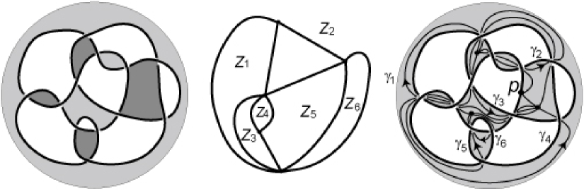
Figure 7. 0214

0258
Generators	$i_{-}(\gamma_{1}),\ldots,i_{-}(\gamma_{4}),\,z_{1},\ldots,z_{7},\,i_{+}(\gamma_{1}),\ldots,i_{+}(\gamma_{4})$
Relations	$z_{1}z_{2}z_{3}z_{4}$, $z_{1}z_{2}z_{4}z_{6}^{-1}z_{7}^{-1}$, $z_{7}z_{6}z_{5}$, $i_{-}(\gamma_{1})z_{7}z_{6}z_{7}^{-1}$,
	$i_{-}(\gamma_{2})z_{7}z_{6}z_{5}^{-1}z_{4}z_{6}^{-1}z_{7}^{-1}$, $i_{-}(\gamma_{3})z_{1}z_{2}^{2}z_{4}^{2}z_{6}^{-1}z_{7}^{-1}$, $i_{-}(\gamma_{4})z_{1}z_{2}^{2}z_{1}^{-2},$
	$i_{+}(\gamma_{1})z_{7}^{-1},\,i_{+}(\gamma_{2})z_{6}z_{4},\,i_{+}(\gamma_{3})z_{2}z_{1}^{-1}z_{4},\,i_{+}(\gamma_{4})z_{2}z_{1}^{-2}\,$
Torsion $\tau^{+}_{\rho_{2}}$	$\displaystyle{-\frac{\gamma_{2}^{5}\gamma_{4}^{7}}{\gamma_{1}^{6}\gamma_{3}^{12}}+\frac{\gamma_{2}^{6}\gamma_{4}^{8}}{\gamma_{1}^{7}\gamma_{3}^{13}}-\frac{\gamma_{2}^{6}\gamma_{4}^{9}}{\gamma_{1}^{7}\gamma_{3}^{14}}}$

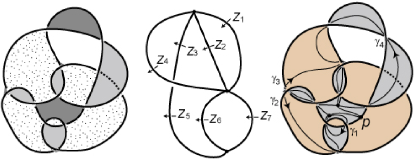
Figure 8. 0258

0279
Generators	$i_{-}(\gamma_{1}),\ldots,i_{-}(\gamma_{4}),\,z_{1},\ldots,z_{9},\,i_{+}(\gamma_{1}),\ldots,i_{+}(\gamma_{4})$
Relations	$z_{1}z_{2}z_{4},\,z_{1}z_{3}^{-1}z_{2}z_{9}^{-1},\,z_{5}z_{8}^{-1}z_{6}^{-1},\,z_{6}z_{7}z_{8}z_{9},\,z_{2}^{-1}z_{3}z_{2}z_{5}^{-1},$
	$i_{-}(\gamma_{1})z_{5}z_{8}z_{2}z_{9}^{-1}z_{5}^{-1},\,i_{-}(\gamma_{2})z_{5}z_{6}^{-1}z_{5}^{-1},\,i_{-}(\gamma_{3})z_{9}^{-1}z_{6}^{-1}z_{5}^{-1},\,i_{-}(\gamma_{4})z_{2}^{-1}z_{3}z_{1}z_{2}^{2},$
	$i_{+}(\gamma_{1})z_{5}z_{2}z_{9}^{-1}z_{5}^{-1},\,i_{+}(\gamma_{2})z_{5}z_{9}z_{6}^{-1},\,i_{+}(\gamma_{3})z_{2}^{-1}z_{6}^{-1},\,i_{+}(\gamma_{4})z_{2}^{-1}z_{1}z_{2}^{2}\,$
Torsion $\tau^{+}_{\rho_{2}}$	$\displaystyle{-\frac{\gamma_{3}^{2}\gamma_{4}^{5}}{\gamma_{2}^{5}}+\frac{\gamma_{3}^{2}\gamma_{4}^{5}}{\gamma_{1}\gamma_{2}^{5}}+\frac{\gamma_{3}^{2}\gamma_{4}^{6}}{\gamma_{2}^{5}}}$

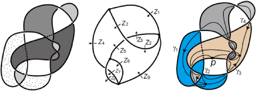
Figure 9. 0279

0382
Generators	$i_{-}(\gamma_{1}),\ldots,i_{-}(\gamma_{4}),\,z_{1},\ldots z_{4},\,i_{+}(\gamma_{1}),\ldots,i_{+}(\gamma_{4})$
Relations	$i_{-}(\gamma_{1})z_{2}z_{1}^{-1}z_{3}z_{2}^{-1},\,i_{-}(\gamma_{2})z_{2}z_{3}^{-1}z_{2}z_{1}^{-2}z_{4}z_{2}^{-1},\,i_{-}(\gamma_{3})z_{4}^{-1}z_{1}^{-1}z_{4}z_{2}^{-1},\,$
	$i_{-}(\gamma_{4})z_{2}^{2}z_{1}^{-1}z_{4},\,$
	$i_{+}(\gamma_{1})z_{3}z_{2}^{-1},\,i_{+}(\gamma_{2})z_{2}z_{1}^{-2}z_{4}z_{1}^{-1},\,i_{+}(\gamma_{3})z_{1}^{-1},\,i_{+}(\gamma_{4})z_{4}z_{2}z_{1}^{-1}z_{4}\,$
Torsion $\tau^{+}_{\rho_{2}}$	$\displaystyle{\frac{1}{\gamma_{1}\gamma_{2}\gamma_{4}}+\frac{1}{\gamma_{1}\gamma_{3}^{2}\gamma_{4}}-\frac{1}{\gamma_{1}\gamma_{3}\gamma_{4}}}$

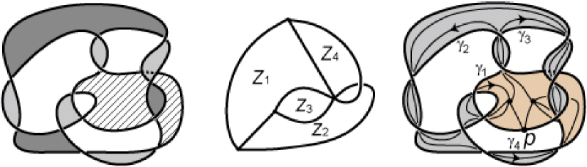
Figure 10. 0382

0394
Generators	$i_{-}(\gamma_{1}),\ldots,i_{-}(\gamma_{4}),\,z_{1},\ldots z_{4},\,i_{+}(\gamma_{1}),\ldots,i_{+}(\gamma_{4})$
Relations	$i_{-}(\gamma_{1})z_{1}^{-1}z_{2}^{-1}z_{3},\,i_{-}(\gamma_{2})z_{3}^{-1}z_{4}z_{2}z_{3}z_{2}^{-1}z_{1},\,i_{-}(\gamma_{3})z_{4}z_{2}z_{3}z_{2}^{-1}z_{1},\,i_{-}(\gamma_{4})z_{4},\,$
	$i_{+}(\gamma_{1})z_{2}^{-1}z_{3},\,i_{+}(\gamma_{2})z_{3}^{-1}z_{1}z_{3}^{-1}z_{4}z_{2}z_{3}z_{2}^{-1},\,i_{+}(\gamma_{3})z_{2}z_{3}z_{2}^{-1},\,i_{+}(\gamma_{4})z_{2}z_{4}\,$
Torsion $\tau^{+}_{\rho_{2}}$	$\displaystyle{\frac{1}{\gamma_{1}\gamma_{2}\gamma_{3}^{2}\gamma_{4}}+\frac{1}{\gamma_{1}^{2}\gamma_{2}\gamma_{3}\gamma_{4}}-\frac{1}{\gamma_{1}\gamma_{2}\gamma_{3}\gamma_{4}}}$

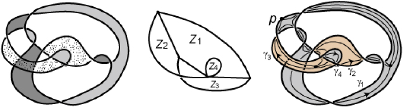
Figure 11. 0394

0464
Generators	$i_{-}(\gamma_{1}),\ldots,i_{-}(\gamma_{4}),\,z_{1},\ldots,z_{10},\,i_{+}(\gamma_{1}),\ldots,i_{+}(\gamma_{4})$
Relations	$z_{1}z_{2}z_{6}z_{7},\,z_{2}z_{9}z_{7},\,z_{3}z_{4}z_{5}z_{10}^{-1},\,z_{4}z_{5}z_{8},\,z_{1}z_{2}z_{3}^{-1}z_{2}^{-1},\,z_{8}z_{6}z_{8}^{-1}z_{9}^{-1},$
	$i_{-}(\gamma_{1})z_{2}z_{10}z_{5}^{-1}z_{9}^{-1}z_{2}^{-1},\,i_{-}(\gamma_{2})z_{2}z_{10}z_{5}^{-1}z_{3}^{-1}z_{2}^{-1},\,i_{-}(\gamma_{3})z_{2}z_{8}^{-1}z_{2}^{-1},\,i_{-}(\gamma_{4})z_{2}z_{1},$
	$i_{+}(\gamma_{1})z_{2}z_{9}^{-1}z_{2}^{-1},\,i_{+}(\gamma_{2})z_{2}z_{5}^{-1}z_{2}^{-1},\,i_{+}(\gamma_{3})z_{1}^{-1}z_{8}^{-1}z_{9}^{-1}z_{2}^{-1}z_{1},\,i_{+}(\gamma_{4})z_{1}^{-1}z_{7}^{-1}z_{1}\,$
Torsion $\tau^{+}_{\rho_{2}}$	$\displaystyle{-\frac{\gamma_{1}^{3}\gamma_{4}^{3}}{\gamma_{3}}-\gamma_{1}^{2}\gamma_{4}^{4}+\gamma_{1}^{3}\gamma_{4}^{4}}$

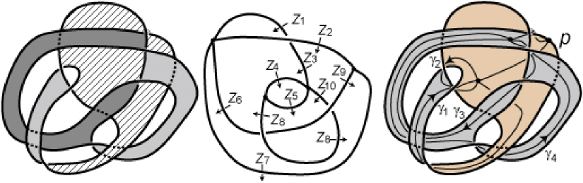
Figure 12. 0464

0483
Generators	$i_{-}(\gamma_{1}),\ldots,i_{-}(\gamma_{4}),\,z_{1},\ldots,z_{9},\,i_{+}(\gamma_{1}),\ldots,i_{+}(\gamma_{4})$
Relations	$z_{8}^{-1}z_{1}z_{4}z_{9}z_{4}^{-1},\,z_{5}z_{6}z_{7}^{-1}z_{6}^{-1}z_{8},\,z_{2}z_{3}z_{2}^{-1}z_{1},\,z_{3}^{-1}z_{2}z_{3}z_{5}^{-1},\,z_{4}z_{9}^{-1}z_{4}^{-1}z_{3},\,$
	$i_{-}(\gamma_{1})z_{1}z_{2}^{-1}z_{1}^{-1},\,i_{-}(\gamma_{2})z_{1}z_{4}^{-1}z_{8}^{-1},\,i_{-}(\gamma_{3})z_{6}^{-1},\,i_{-}(\gamma_{4})z_{6}^{-1}z_{3},$
	$i_{+}(\gamma_{1})z_{4}^{-1}z_{2}^{-1},\,i_{+}(\gamma_{2})z_{4}^{-1},\,i_{+}(\gamma_{3})z_{5}z_{6}^{-1}z_{8},\,i_{+}(\gamma_{4})z_{8}^{-1}z_{3}$
Torsion $\tau^{+}_{\rho_{2}}$	$\displaystyle{\frac{1}{\gamma_{1}\gamma_{3}\gamma_{4}^{2}}-\frac{\gamma_{2}}{\gamma_{1}^{2}\gamma_{3}\gamma_{4}^{2}}-\frac{1}{\gamma_{1}\gamma_{3}\gamma_{4}}}$

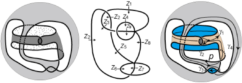
Figure 13. 0483

0535
Generators	$i_{-}(\gamma_{1}),\ldots,i_{-}(\gamma_{4}),\,z_{1},\ldots,z_{10},\,i_{+}(\gamma_{1}),\ldots,i_{+}(\gamma_{4})$
Relations	$z_{1}z_{2}z_{3},\,z_{2}z_{6}z_{7}^{-1},\,z_{10}^{-1}z_{4}z_{5}z_{8}^{-1}z_{7},\,z_{1}z_{10}z_{9},\,z_{2}z_{3}z_{2}^{-1}z_{4}^{-1},\,z_{2}z_{6}^{-1}z_{2}^{-1}z_{5}^{-1},$
	$i_{-}(\gamma_{1})z_{10}^{-1},\,i_{-}(\gamma_{2})z_{10}^{-1}z_{1}^{-1}z_{3}^{-1}z_{1}^{-1}z_{10},\,i_{-}(\gamma_{3})z_{7}^{-1}z_{1}^{-1}z_{10},\,i_{-}(\gamma_{4})z_{6}z_{3}^{-1}z_{7},$
	$i_{+}(\gamma_{1})z_{7}^{-1}z_{9},\,i_{+}(\gamma_{2})z_{7}^{-1}z_{1}^{-1}z_{3}^{-1}z_{10}z_{7},\,i_{+}(\gamma_{3})z_{7}^{-1}z_{3}z_{10}z_{7},\,i_{+}(\gamma_{4})z_{7}^{-1}z_{6}z_{3}^{-1}z_{7}$
Torsion $\tau^{+}_{\rho_{2}}$	$\displaystyle{-\frac{1}{\gamma_{1}^{11}\gamma_{2}^{6}\gamma_{3}^{6}\gamma_{4}^{15}}+\frac{1}{\gamma_{1}^{10}\gamma_{2}^{5}\gamma_{3}^{6}\gamma_{4}^{15}}-\frac{1}{\gamma_{1}^{10}\gamma_{2}^{5}\gamma_{3}^{6}\gamma_{4}^{14}}}$

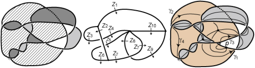
Figure 14. 0535

0650
Generators	$i_{-}(\gamma_{1}),\ldots,i_{-}(\gamma_{4}),\,z_{1},\ldots,z_{11},\,i_{+}(\gamma_{1}),\ldots,i_{+}(\gamma_{4})$
Relations	$z_{2}z_{3}z_{1}^{-1}z_{4}z_{1},\,z_{2}z_{6}z_{8}^{-1}z_{6}^{-1}z_{11}^{-1},\,z_{1}z_{5}^{-1}z_{1}^{-1}z_{4},\,z_{3}z_{6}z_{9}^{-1}z_{6}^{-1},\,z_{9}z_{8}^{-1}z_{7}z_{8},\,$
	$z_{8}z_{7}z_{10}^{-1}z_{7}^{-1},\,z_{10}z_{6}^{-1}z_{11}z_{6},$
	$i_{-}(\gamma_{1})z_{2}z_{6}^{-1}z_{2}^{-1},\,i_{-}(\gamma_{2})z_{2}z_{7}z_{6}^{-1}z_{2}^{-1},\,i_{-}(\gamma_{3})z_{6}z_{8}z_{6}^{-1}z_{2}^{-1},\,i_{-}(\gamma_{4})z_{2}z_{3}z_{1}^{-1},$
	$i_{+}(\gamma_{1})z_{11}z_{6}^{-1}z_{2}^{-1},\,i_{+}(\gamma_{2})z_{2}z_{3}^{-1}z_{2}^{-1},\,i_{+}(\gamma_{3})z_{1}z_{6}z_{8}z_{6}^{-1},\,i_{+}(\gamma_{4})z_{1}^{-1}$
Torsion $\tau^{+}_{\rho_{2}}$	$\displaystyle{\frac{1}{\gamma_{1}\gamma_{2}^{3}\gamma_{3}^{2}\gamma_{4}^{2}}-\frac{1}{\gamma_{1}\gamma_{2}^{3}\gamma_{3}\gamma_{4}}+\frac{1}{\gamma_{1}\gamma_{2}^{2}\gamma_{3}\gamma_{4}}}$

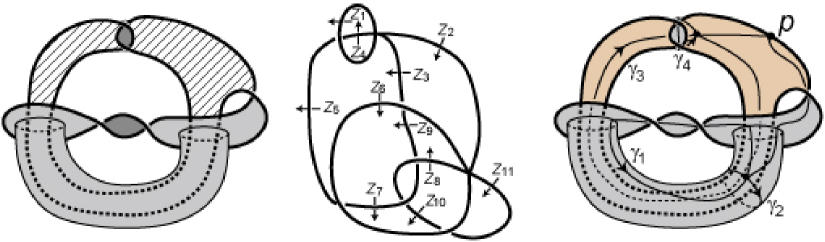
Figure 15. 0650

0801
Generators	$i_{-}(\gamma_{1}),\ldots,i_{-}(\gamma_{4}),\,z_{1},\ldots,z_{9},\,i_{+}(\gamma_{1}),\ldots,i_{+}(\gamma_{4})$
Relations	$z_{1}^{-1}z_{6}z_{7}z_{8}^{-1}z_{9}^{-1},\,z_{3}z_{4}z_{9}z_{6}^{-1},\,z_{2}z_{4}z_{5},\,z_{2}z_{6}z_{7}^{-1}z_{6}^{-1},\,z_{2}z_{3}^{-1}z_{2}^{-1}z_{1},$
	$i_{-}(\gamma_{1})z_{6}z_{7}z_{8}^{-1}z_{6},\,i_{-}(\gamma_{2})z_{1}z_{2}z_{8}z_{7}^{-1}z_{6}^{-1},\,i_{-}(\gamma_{3})z_{9}z_{6}^{-1}z_{2}^{-1},\,i_{-}(\gamma_{4})z_{5}^{-1}z_{9}^{-1}z_{5}^{-1},$
	$i_{+}(\gamma_{1})z_{6}z_{9},\,i_{+}(\gamma_{2})z_{6}z_{2}z_{6}z_{9}^{-1}z_{6}^{-1},\,i_{+}(\gamma_{3})z_{5}z_{9}z_{6}^{-1},\,i_{+}(\gamma_{4})z_{4}z_{9}^{-1}z_{5}^{-1}$
Torsion $\tau^{+}_{\rho_{2}}$	$-\gamma_{1}^{2}\gamma_{3}^{2}\gamma_{4}+\gamma_{1}^{2}\gamma_{2}\gamma_{3}^{2}\gamma_{4}-\gamma_{1}^{2}\gamma_{2}\gamma_{3}^{3}\gamma_{4}^{2}$

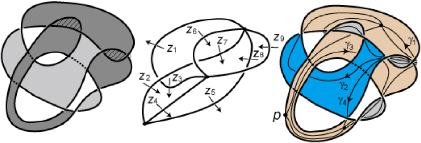
Figure 16. 0801

0815
Generators	$i_{-}(\gamma_{1}),\ldots,i_{-}(\gamma_{4}),\,z_{1},\ldots,z_{11},\,i_{+}(\gamma_{1}),\ldots,i_{+}(\gamma_{4})$
Relations	$z_{1}z_{9}z_{6},\,z_{1}z_{2}^{-1}z_{4}^{-1},\,z_{4}z_{11}^{-1}z_{5},\,z_{10}^{-1}z_{5}^{-1}z_{6}z_{7}z_{8},\,z_{8}^{-1}z_{6}^{-1}z_{9}z_{6},\,$
	$z_{7}^{-1}z_{6}^{-1}z_{3}z_{6},\,z_{4}z_{3}^{-1}z_{4}^{-1}z_{10},$
	$i_{-}(\gamma_{1})z_{4}z_{3}^{-1}z_{4}^{-1},\,i_{-}(\gamma_{2})z_{4}z_{11},\,i_{-}(\gamma_{3})z_{9},\,i_{-}(\gamma_{4})z_{2}^{-1}z_{9}^{-1},$
	$i_{+}(\gamma_{1})z_{2}^{-1}z_{3}^{-1}z_{4}^{-1},\,i_{+}(\gamma_{2})z_{11}z_{1},\,i_{+}(\gamma_{3})z_{9}z_{3}^{-1}z_{1},\,i_{+}(\gamma_{4})z_{9}z_{2}^{-1}z_{9}^{-1}$
Torsion $\tau^{+}_{\rho_{2}}$	$\displaystyle{-\frac{\gamma_{1}^{3}\gamma_{2}^{5}}{\gamma_{4}^{6}}+\frac{\gamma_{1}^{2}\gamma_{2}^{4}}{\gamma_{4}^{5}}+\frac{\gamma_{1}^{3}\gamma_{2}^{5}}{\gamma_{4}^{5}}}$

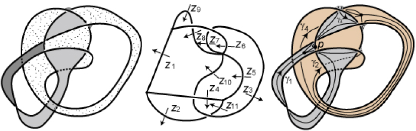
Figure 17. 0815

Remark 5.1.

According to [1] and [21], these knots have unique minimal genus Seifert surfaces.

6. Magnus matrix and concordances of Seifert surfaces

Not only the torsion $\tau_{\rho}^{+}$ but the Magnus matrix $r_{\rho}$ can be used as a fibering obstruction of homologically fibered knots. In fact, for a fibered knot $K$ with its unique minimal genus Seifert surface $R$ of genus $g$, the sutured manifold $M_{R}$ is given by a mapping cylinder $(\Sigma_{g,1}\times[0,1],\mathrm{id}\times 1,\varphi\times 0)$ of $\varphi$, which is an element of the mapping class group of $\Sigma_{g,1}$ and is uniquely (not up to conjugation) determined after fixing an identification of $R$ with $\Sigma_{g,1}$. Then the Magnus matrix $r_{\rho}(M_{R})$ associated with a homomorphism $\rho:G(K)\to\Gamma$ is given by $\overline{\sideset{{}^{\rho\circ i_{+}}\!}{}{\mathop{\left({\displaystyle\frac{\partial\varphi(\gamma_{j})}{\partial\gamma_{i}}}\right)}\nolimits}}_{1\leq i,j\leq 2g}$. In particular, all the entries are elements of $\mathbb{Z}\Gamma$. Therefore, for the detection of non-fiberedness of a non-fibered homologically fibered knot $K$, it suffices to find a minimal genus Seifert surface $R$, an identification of $R$ with $\Sigma_{g,1}$ and a homomorphism $\rho:G(K)\to\Gamma$ to a PTFA group $\Gamma$ whose Magnus matrix has an entry not contained in $\mathbb{Z}\Gamma$.

Example 6.1.

If we continue the computation for the knot 0057 in Section 4, we can see that the $(1,3)$-entry of $r_{\rho_{2}}(M_{R})$ is $\displaystyle\frac{\gamma_{4}}{1+\gamma_{2}-\gamma_{2}\gamma_{4}}$, not an element of $\mathbb{Z}D_{2}(K)$. This shows that the knot 0057 is not fibered.

In the usage of $r_{\rho}$ as a fibering obstruction, its invariance under homology cobordisms of homology cylinders is convenient. We first recall the definition of homology cobordisms of homology cylinders:

Definition 6.2.

Two homology cylinders $M=(M,i_{+},i_{-}),N=(N,j_{+},j_{-})\in\mathcal{C}_{g,1}$ are said to be $($rational$)$ homology cobordant if there exists a smooth compact oriented 4-manifold $W$ such that:

1. $\partial W=M\cup(-N)/(i_{+}(x)=j_{+}(x),\,i_{-}(x)=j_{-}(x))\quad x\in\Sigma_{g,1}$; and

2. the inclusions $M\hookrightarrow W$, $N\hookrightarrow W$ induce isomorphisms on the (rational) homology,

where $-N$ denotes $N$ with opposite orientation.

Proposition 6.3.

Suppose that $M=(M,i_{+},i_{-}),N=(N,j_{+},j_{-})\in\mathcal{C}_{g,1}^{\mathbb{Q}}$ are rational homology cobordant by a rational homology cobordism $W$. Let $\rho:\pi_{1}(W)\to\Gamma$ be a homomorphism to a PTFA group. Then the Magnus matrices $r_{\rho}(M)$ and $r_{\rho}(N)$ associated with $\pi_{1}(M)\to\pi_{1}(W)\xrightarrow{\rho}\Gamma$ and $\pi_{1}(N)\to\pi_{1}(W)\xrightarrow{\rho}\Gamma$ are defined, and $r_{\rho}(M)=r_{\rho}(N)$ holds.

Proof.

We can apply the argument of [29, Section 3.1] and we omit the details. ∎

To interpret the homology cobordant relation in terms of homologically fibered knots, we introduce concordances of Seifert surfaces defined by Myers.

Definition 6.4 (Myers [27]).

Seifert surfaces $R$, $R^{\prime}$ of genus $g$ for knots $K$, $K^{\prime}$ in $S^{3}$ are said to be concordant if there is a smooth embedding $I:\Sigma_{g,1}\times[0,1]\to S^{3}\times[0,1]$ such that $I(\Sigma_{g,1}\times\{0\})=R$ and $I(\Sigma_{g,1}\times\{1\})=R^{\prime}$.

Using this terminology, we have the following relationship between concordances of Seifert surfaces for homologically fibered knots and homology cylinders.

Proposition 6.5.

Let $K$ be a $($rationally$)$ homologically fibered knot with a minimal genus Seifert surface $R$ of genus $g$. Suppose $R$ is concordant to another Seifert surface $R^{\prime}$ of a knot $K^{\prime}$. Then $K^{\prime}$ is also a $($rationally$)$ homologically fibered knot of genus $g$ with a minimal genus Seifert surface $R^{\prime}$ such that $M_{R}$ and $M_{R^{\prime}}$ are $($rational$)$ homology cobordant as $($rational$)$ homology cylinders.

Proof.

Let $W$ be a manifold obtained from $S^{3}\times[0,1]$ by cutting along the image of an embedding $I:\Sigma_{g,1}\times[0,1]\to S^{3}\times[0,1]$ which connects $R$ and $R^{\prime}$. Then it is straightforward to check our assertions by observing the Mayer-Vietoris exact sequence of $S^{3}\times[0,1]=W\cup I(\Sigma_{g,1}\times[0,1])$ with the intersection homeomorphic to $(\partial M_{R})\times[0,1]=(\Sigma_{g,1}\cup(-\Sigma_{g,1}))\times[0,1]$. We omit the details. ∎

The following theorem enables us to produce infinitely many Seifert surfaces which are concordant to a given one.

Theorem 6.6 (Myers [27]).

If a Seifert surface $R$ of a knot $K$ is not a disk, then $R$ is concordant to $R^{\prime}$ such that:

• $K^{\prime}=\partial R^{\prime}$ is hyperbolic; and

• $S^{3}-K^{\prime}$ has arbitrarily large hyperbolic volume.

For $(M,i_{+},i_{-})\in\mathcal{C}_{g,1}$, consider a homomorphism

$$\rho_{M}:\pi_{1}(M)\to H_{1}(M)\xrightarrow{i_{+}^{-1}}H_{1}(\Sigma_{g,1}).$$

We can easily check that if $W$ is a homology cobordism between $M$ and $N$ in $\mathcal{C}_{g,1}$, then there exists an extension $\rho_{W}:\pi_{1}(W)\to H_{1}(\Sigma_{g,1})$ of $\rho_{M}$ and $\rho_{N}$. Note that $\rho_{M}$ can be regarded as a restriction of $\rho_{2}$ when $M$ is obtained from a homologically fibered knot (recall the exact sequence (4.1)). Consequently we can combine Theorem 6.6 with Proposition 6.3 as follows:

Theorem 6.7.

Let $K$ be a homologically fibered knot with a minimal genus Seifert surface $R$. If $K$ is shown to be non-fibered by using $r_{\rho_{2}}(M_{R})(=r_{\rho_{M_{R}}}(M_{R}))$, then $K^{\prime}=\partial R^{\prime}$ is also non-fibered for any Seifert surface $R^{\prime}$ concordant to $R$. Moreover, there exist infinitely many such $K^{\prime}=\partial R^{\prime}$.

We may take $K$ to be a homologically fibered knot in Section 4. Then Theorem 6.7 shows that there does exist infinitely many homologically fibered knots whose non-fiberedness are detected by the Magnus matrices.

Example 6.8.

Let $K$ be the knot as the boundary of the Seifert surface $R$ illustrated in Figure 18.

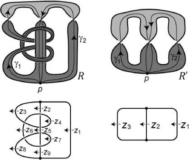
Figure 18. Concordant Seifert surfaces

$R$ is concordant to the minimal genus Seifert surface $R^{\prime}$ of the trefoil knot, which is fibered. Proposition 6.5 shows that $K$ is a homologically fibered knot and $R$ is of minimal genus. An admissible presentation of $\pi_{1}(M_{R})$ is given by

Generators	$i_{-}(\gamma_{1}),\,i_{-}(\gamma_{2}),\,z_{1},\ldots,z_{9},\,i_{+}(\gamma_{1}),\,i_{+}(\gamma_{2})$
Relations	$z_{1}z_{2}z_{3},\,z_{1}z_{9}z_{8},\,z_{4}z_{5}z_{4}^{-1}z_{2}^{-1},\,z_{4}^{-1}z_{5}z_{3}^{-1}z_{5}^{-1},\,z_{3}z_{6}z_{3}^{-1}z_{4},\,z_{7}z_{5}z_{8}z_{5}^{-1}$,
	$z_{7}^{-1}z_{9}z_{7}z_{5}^{-1},\,i_{-}(\gamma_{1})z_{1}z_{7}z_{4}^{-1}z_{2}z_{5}^{-1}z_{3}z_{8}^{-1}z_{5},\,i_{-}(\gamma_{2})z_{8}^{-1}z_{7}z_{4}^{-1}z_{1}^{-1},$
	$i_{+}(\gamma_{1})z_{7}z_{4}^{-1}z_{2}z_{5}^{-1}z_{3}z_{8}^{-1}z_{5},\ i_{+}(\gamma_{2})z_{7}z_{4}^{-1}z_{1}^{-1}.$

From this, we have

$$\det(\tau_{\rho_{2}}^{+}(M_{R})) =3-\frac{1}{\gamma_{1}}-\gamma_{1}-\frac{\gamma_{1}}{\gamma_{2}}+\frac{\gamma_{1}^{2}}{\gamma_{2}}+\frac{\gamma_{2}}{\gamma_{1}^{2}}-\frac{\gamma_{2}}{\gamma_{1}},$$

$$r_{\rho_{2}}(M_{R}) =\begin{pmatrix}1&\gamma_{2}^{-1}\\ -\gamma_{1}^{-1}\gamma_{2}&1-\gamma_{1}^{-1}\end{pmatrix}.$$

On the other hand, an admissible presentation of $\pi_{1}(M_{R^{\prime}})$ is given by

Generators	$i_{-}(\gamma_{1}),\,i_{-}(\gamma_{2}),\,z_{1},\,z_{2},\,z_{3},\,i_{+}(\gamma_{1}),\,i_{+}(\gamma_{2})$
Relations	$z_{1}z_{2}z_{3},\,i_{-}(\gamma_{1})z_{3}^{-1},\,i_{-}(\gamma_{2})z_{3}^{-1}z_{1}^{-1},\,i_{+}(\gamma_{1})z_{2},\,i_{+}(\gamma_{2})z_{1}^{-1}$

and we have

$$\det(\tau_{\rho_{2}}^{+}(M_{R})) =\frac{1}{\gamma_{2}},$$

$$r_{\rho_{2}}(M_{R}) =\begin{pmatrix}1&\gamma_{2}^{-1}\\ -\gamma_{1}^{-1}\gamma_{2}&1-\gamma_{1}^{-1}\end{pmatrix}.$$

Remark 6.9.

As seen in Example 6.8, $\Gamma$-torsion generally changes under homology cobordisms. However, Cha-Friedl-Kim [2] recently found a way to extract homology cobordant invariants from the torsion $\tau_{\rho_{2}}^{+}$ by taking a certain quotient of the target. Then they applied it to the homology cobordism group of homology cylinders and showed that this group has $\mathbb{Z}_{2}^{\infty}$ as an abelian quotient. By Proposition 2.5, we may regard this abelian quotient as an invariant of homologically fibered knots. In fact, it is unchanged under concordances of Seifert surfaces.

7. MATHEMATICA program

The following is a MATHEMATICA program which calculates the invariants discussed in Sections 4, 5 and 6.

h1Class = {};
h1Monodromy = {};
torsionMatrix = {};
magnusMatrix = {};

invariants[g_, z_, RELATIONS_] :=
  Module[{reindexedRel, h1Matrix, i, alex},
   GENUS = g;
   Ztotal = z;

   reindexedRel = Map[reindexing, RELATIONS, {2}];

   h1Matrix = -Map[Take[#, -2 GENUS] &, homologyComputation[reindexedRel]];
   h1Class =
    Join[Map[monomialExpression, h1Matrix],
     Table[ToExpression[ToString[SequenceForm["\[Gamma]", i]]], {i, 2 GENUS}]];
   Print["Homology classes of generators = ", h1Class // DisplayForm];

   h1Monodromy = Transpose[Take[h1Matrix, 2 GENUS]];
   Print["Homological monodromy = ", h1Monodromy // MatrixForm];

   alex = Transpose[makeAlexanderMatrix[reindexedRel]];
   torsionMatrix = Take[alex, 2 GENUS + Ztotal];
   Print["torsion matrix = ", torsionMatrix // MatrixForm];
   Print["det(torsion) = ", Expand[Det[torsionMatrix]]];

   magnusMatrix = Simplify[Transpose[
     Take[Transpose[-Drop[alex, 2 GENUS + Ztotal].Inverse[
           torsionMatrix]], 2 GENUS]]];
   Print["Magnus matrix = ", magnusMatrix // MatrixForm]
   ];

reindexing[num_] :=
  Module[{numString, sg},
    If[NumberQ[num], num + 2 GENUS*Sign[num],
     numString = ToString[num];
     sg = If[StringTake[numString, 1] == "-", 1, 0];
     If[StringTake[numString, {1 + sg}] == "m",
      ((-1)^sg)*ToExpression[StringDrop[numString, 1 + sg]],
      ((-1)^sg)*(ToExpression[StringDrop[numString, 1 + sg]] + 2 GENUS + Ztotal)]]
   ];

homologyComputation[rel_] :=
  Module[{i, j},
   RowReduce[Table[Count[rel[[i]], j] - Count[rel[[i]], -j],
   {i, 1, 2 GENUS + Ztotal}, {j, 1, 4 GENUS + Ztotal}]]];

monomialExpression[list_] :=
  Module[{i, prod = 1},
   For[i = 1, i <= 2 GENUS, i++,
    prod = prod*(ToExpression[ToString[SequenceForm["\[Gamma]", i]]]^list[[i]])];
   prod];

makeAlexanderMatrix[rel_] :=
  Module[{i, j},
   Table[foxDer[rel[[i]], j], {i, 1, Length[rel]}, {j, 1, 4 GENUS + Ztotal}]];

foxDer[word_, var_] :=
  Module[{entry = 0, i},
   For[i = 1, i <= Length[word], i++,
    Which[word[[i]] == var,
     entry = entry + (makeMonomial[Take[word, i - 1]]^(-1)),
     word[[i]] == -var,
     entry = entry - (makeMonomial[Take[word, i]]^(-1))]];
   entry];

makeMonomial[list_] :=
  Module[{prod = 1},
   For[i = 1, i <= Length[list], i++,
    prod = prod*(h1Class[[Abs[list[[i]]]]]^Sign[list[[i]]])];
   prod];

A computation by this program goes as follows. Let $(M,i_{+},i_{-})\in\mathcal{C}_{g,1}$ with an admissible presentation

$$\langle i_{-}(\gamma_{1}),\ldots,i_{-}(\gamma_{2g}),z_{1},\ldots,z_{l},i_{+}(\gamma_{1}),\ldots,i_{+}(\gamma_{2g})\mid r_{1},\ldots,r_{2g+l}\rangle$$

of $\pi_{1}(M)$. The main function in the program is $\mathtt{invariants}$ having three slots as the input. These slots correspond to the genus $g$, the number $l$ of $z$-generators and the list of relations. For each word in the relations, we make a list by replacing $i_{-}(\gamma_{j})^{\pm 1}$, $z_{j}^{\pm 1}$ and $i_{+}(\gamma_{j})^{\pm 1}$ by $\pm\mathtt{mj}$, $\pm\mathtt{j}$ and $\pm\mathtt{pj}$. By lining up them, we obtain the list of relations.

When we compute the case of the knot 0815 with an admissible presentation of $\pi_{1}(M_{R})$ of the sutured manifold $M_{R}$ as in Section 5, for example, the input is:

invariants[2, 11, {{1, 9, 6}, {1, -2,-4}, {4,-11, 5},
  {-10, -5, 6, 7, 8}, {-8, -6, 9, 6}, {-7, -6, 3, 6},
  {4, -3, -4, 10}, {m1, 4, -3, -4}, {m2, 4, 11},
  {m3, 9}, {m4, -2, -9}, {p1, -2, -3, -4}, {p2, 11, 1},
  {p3, 9, -3, 1}, {p4, 9, -2, -9}}]

Then the function returns homology classes of generators in terms of $\mathtt{\gamma j}:=i_{+}(\gamma_{j})\in H_{1}(M_{R})$, the homological monodromy matrix $\sigma(M_{R})$, the torsion matrix $\tau_{\rho_{2}}^{+}(M_{R})$ and the Magnus matrix $r_{\rho_{2}}(M_{R})$. These data can be referred as the variables $\mathtt{h1Class}$, $\mathtt{h1Monodromy}$, $\mathtt{torsionMatrix}$ and $\mathtt{magnusMatrix}$.

References

- [1] J. Baldwin, W. Gillam, Computations of Heegaard-Floer knot homology, preprint, arXiv:0610167.
- [2] J. Cha, S. Friedl, T Kim, The cobordism group of homology cylinders, preprint, arXiv:0909.5580.
- [3] J. Cha, C. Livingston, Table of Knot Invariants, http://www.indiana.edu/~knotinfo/.
- [4] T. Cochran, Noncommutative knot theory, Algebr. Geom. Topol. 4 (2004), 347–398.
- [5] T. Cochran, K. Orr, P. Teichner, Knot concordance, Whitney towers and -signatures, Ann. of Math. 157 (2003), 433–519.
- [6] R. Crowell, H. Trotter, A class of pretzel knots, Duke Math. J. 30 (1963), 373–377.
- [7] J. Eisner, Knots with infinitely many minimal spanning surfaces, Trans. Amer. Math. Soc. 229 (1977), 329–349.
- [8] S. Friedl, Reidemeister torsion, the Thurston norm and Harvey’s invariants, Pacific J. Math. 230 (2007), 271–296.
- [9] S. Friedl, A. Juhász, J. Rasmussen, The decategorification of sutured Floer homology, preprint, arXiv:0903.5287.
- [10] S. Friedl, T. Kim, The Thurston norm, fibered manifolds and twisted Alexander polynomials, Topology 45 (2006), 929–953.
- [11] D. Gabai, Foliations and the topology of -manifolds, J. Differential Geom. 18 (1983), 445–503.
- [12] S. Garoufalidis, J. Levine, Tree-level invariants of three-manifolds, Massey products and the Johnson homomorphism, Graphs and patterns in mathematics and theorical physics, Proc. Sympos. Pure Math. 73 (2005), 173–205.
- [13] H. Goda, H. Matsuda, A. Pajitnov, Morse-Novikov theory, Heegaard splittings and closed orbits of gradient flows, preprint, arXiv:0709.3153.
- [14] H. Goda, T. Sakasai, Homology cylinders in knot theory, preprint, arXiv:0807.4034.
- [15] H. Goda, T. Sakasai, Johnson homomorphisms and homologically fibered knots, in preparation.
- [16] M. Goussarov, Finite type invariants and -equivalence of -manifolds, C. R. Math. Acad. Sci. Paris 329 (1999), 517–522.
- [17] K. Habiro, Claspers and finite type invariants of links, Geom. Topol. 4 (2000), 1–83.
- [18] S. Harvey, Monotonicity of degrees of generalized Alexander polynomials of groups and 3-manifolds, Math. Proc. Cambridge Philos. Soc. 140 (2006), 431–450.
- [19] M. Hutchings, Y-J. Lee, Circle-valued Morse theory, Reidemeister torsion, and Seiberg- Witten invariants of 3-manifolds, Topology 38 (1999), 861–888.
- [20] M. Hutchings, Y-J. Lee, Circle-valued Morse theory and Reidemeister torsion, Geom. Topol. 3 (1999), 369–396.
- [21] A. Juhász, Knot Floer homology and Seifert surfaces, Algebr. Geom. Topol. 8 (2008), 603–608.
- [22] P. Kirk, C. Livingston, Z. Wang, The Gassner representation for string links, Commun. Contemp. Math. 3 (2001), 87–136.
- [23] T. Kitayama, Non-commutative Reidemeister torsion and Morse-Novikov theory, Proc. Amer. Math. Soc. 138 (2010), 3345–3360.
- [24] J. Levine, Homology cylinders: an enlargement of the mapping class group, Algebr. Geom. Topol. 1 (2001), 243–270.
- [25] J. Milnor, A duality theorem for Reidemeister torsion, Ann. of Math. 76 (1962), 137–147.
- [26] J. Milnor, Whitehead torsion, Bull. Amer. Math. Soc. 72 (1966), 358–426.
- [27] R. Myers, Concordance of Seifert surfaces, in preparation.
- [28] D. Passman, The Algebraic Structure of Group Rings, John Wiley and Sons, 1977.
- [29] T. Sakasai, The Magnus representation and higher-order Alexander invariants for homology cobordisms of surfaces, Algebr. Geom. Topol. 8 (2008), 803–848.
- [30] M. Scharlemann, A. Thompson, Finding disjoint Seifert surfaces, Bull. London Math. Soc. 20 (1988), 61–64.
- [31] R. Strebel, Homological methods applied to the derived series of groups, Comment. Math. Helv. 49 (1974), 302–332.