Neutralino, axion and axino cold dark matter
in minimal, hypercharged and gaugino AMSB
Howard Baer1111Email: baer@nhn.ou.edu ,
Radovan Dermíšek2222Email: dermisek@indiana.edu,
Shibi Rajagopalan1333Email: shibi@nhn.ou.edu,
Heaya Summy1444Email: heaya@nhn.ou.edu
1. Dept. of Physics and Astronomy,
University of Oklahoma, Norman, OK 73019, USA
2. Dept. of Physics,
Indiana University, Bloomington IN 47405, USA
Supersymmetric models based on anomaly-mediated SUSY breaking (AMSB) generally give rise to a neutral wino as a WIMP cold dark matter (CDM) candidate, whose thermal abundance is well below measured values. Here, we investigate four scenarios to reconcile AMSB dark matter with the measured abundance: 1. non-thermal wino production due to decays of scalar fields (e.g. moduli), 2. non-thermal wino production due to decays of gravitinos, 3. non-thermal wino production due to heavy axino decays, and 4. the case of an axino LSP, where the bulk of CDM is made up of axions and thermally produced axinos. In cases 1 and 2, we expect wino CDM to constitute the entire measured DM abundance, and we investigate wino-like WIMP direct and indirect detection rates. Wino direct detection rates can be large, and more importantly, are bounded from below, so that ton-scale noble liquid detectors should access all of parameter space for GeV. Indirect wino detection rates via neutrino telescopes and space-based cosmic ray detectors can also be large. In case 3, the DM would consist of an axion plus wino admixture, whose exact proportions are very model dependent. In this case, it is possible that both an axion and a wino-like WIMP could be detected experimentally. In case 4., we calculate the re-heat temperature of the universe after inflation. In this case, no direct or indirect WIMP signals should be seen, although direct detection of relic axions may be possible. For each DM scenario, we show results for the minimal AMSB model, as well as for the hypercharged and gaugino AMSB models.
1 Introduction
Supersymmetric (SUSY) models of particle physics are very attractive in that they stabilize the gauge hierarchy problem, and provide an avenue for the incorporation of gravity via local SUSY, or supergravity[1]. They also receive some indirect experimental support via the unification of gauge couplings under Minimal Supersymmetric Standard Model (MSSM) renormalization group evolution (RGE)[2], and they provide several different candidates (neutralinos, gravitinos, axions/axinos, ) which can serve as cold dark matter (CDM) in the universe. If evidence for SUSY is found at LHC, then a paramount question will be: what is the mechanism of SUSY breaking, and how is it communicated to the visible sector? Some of the possibilities proposed in the literature include: gravity-mediation (SUGRA) with a gravitino mass TeV[4], gauge-mediation (GMSB) with TeV[5], and anomaly mediation (AMSB) with TeV[6, 7, 8].
Anomaly-mediated supersymmetry breaking (AMSB) models have received much attention in the literature due to their attractive properties[6, 7]: 1. the soft supersymmetry (SUSY) breaking terms are completely calculable in terms of just one free parameter (the gravitino mass, ), 2. the soft terms are real and flavor invariant, thus solving the SUSY flavor and problems and 3. the soft terms are actually renormalization group invariant[9], and can be calculated at any convenient scale choice. In order to realize the AMSB set-up, it was proposed that the hidden sector be “sequestered” on a separate brane from the observable sector in an extra-dimensional universe, so that tree-level supergravity breaking terms do not dominate the soft term contributions. Such a set-up can be realized in brane-worlds, where SUSY breaking takes place on one brane, with the visible sector residing on a separate brane.
A further attractive feature of AMSB models arises due to the scale of their gravitino mass. SUGRA-type models with TeV suffer from the cosmological gravitino problem. There are two parts to the gravitino problem[10]. 1. If the re-heat temperature after inflation GeV, then the high rate of thermal gravitino production leads to an overabundance of neutralino dark matter[11]. 2. Even for lower values of GeV, thermal production of followed by late decays to pairs injects high energy particles into the cosmic soup during or after BBN, thus disrupting one of the pillars of Big-Bang theory[11]. If 5 TeV, then the lifetime drops below sec, and gravitino decay occurs before or at the onset of BBN. In AMSB models where TeV, the gravitino is much too short-lived to be afflicted by the BBN bounds.
In spite of their attractive features, AMSB models suffer from the well-known problem that slepton mass-squared parameters are found to be negative, giving rise to tachyonic states. The original “solution” to this problem was to posit that scalars acquire as well a universal mass , which when added to the AMSB SSB terms, renders them positive[6, 7]. The derived form of soft SUSY breaking terms, supplemented by a universal scalar mass and implemented at the GUT scale, constitutes what is usually called the minimal AMSB, or mAMSB model. In mAMSB and the additional models described below, it is assumed that electroweak symmetry is broken radiatively due to the large top quark mass, so that the magnitude of the parameter is determined to gain the correct value of , and the bilinear soft term is traded for the ratio of Higgs field vevs, .
An alternative set-up for AMSB has been advocated in Ref. [12], known as hypercharged anomaly-mediation (HCAMSB). It is a string-motivated scenario which uses a similar setup as the one envisioned for AMSB. In HCAMSB, the MSSM resides on a D-brane, and the hypercharge gaugino mass is generated in a geometrically separated hidden sector. An additional contribution to the gaugino mass is generated, and its magnitude is parametrized by an additional parameter . The large value of feeds into slepton mass evolution through the MSSM RGE, and acts to lift the weak-scale slepton soft masses beyond tachyonic values. Thus, the HCAMSB model naturally solves the tachyonic slepton mass problem which is endemic to pure AMSB scenarios.
A third scenario has recently been proposed in Ref. [13], under the name gaugino AMSB, or inoAMSB. The inoAMSB model is suggested by recent work on the phenomenology of flux compactified type IIB string theory[14], which reduces to supergravity below the compactification scale. The essential features of this scenario are that the gaugino masses are of the anomaly-mediated SUSY breaking (AMSB) form, while scalar and trilinear soft SUSY breaking terms are highly suppressed: they are taken as at energy scale , at first approximation. The normally large value of as generated in AMSB models feeds into the scalar soft term evolution, lifting slepton soft masses to generate an allowable sparticle mass spectrum, while at the same time avoiding tachyonic sleptons or charged LSPs (lightest SUSY particles). Charged LSPs are common in models with negligible soft scalar masses, such as no-scale[15] or gaugino mediation models[16]. Since scalar and trilinear soft terms are highly suppressed, the SUSY induced flavor and -violating processes are also suppressed in inoAMSB.
All three of these models– mAMSB, HCAMSB and inoAMSB– share the common feature that the lightest MSSM particle is a neutral wino, while the lightest chargino is wino-like with a mass . The - mass gap is of order MeV[17], so that dominantly , with the decay-produced pion(s) being very soft. The small mass gap makes the rather long lived ( sec), and it may yield observable highly ionizing tracks (HITs) of order in length at LHC detectors[32].
An important consequence of wino-like neutralinos is that the thermal abundance of neutralino cold dark matter falls generally an order of magnitude or so below the measured abundance:
| (1) |
according to the WMAP7 data analysis[18]. This latter fact has led many to consider AMSB-like models as perhaps less interesting than SUGRA-type models, wherein the bino-like or mixed bino-higgsino neutralino can more easily yield the measured relic abundance.
In this paper, we address the question of the dark matter abundance in AMSB models. While the calculated thermal abundance of wino-like neutralinos is found to be below measured values (for GeV), we find that there exists a variety of attractive methods to augment the wino abundance, thus bringing the calculated abundance into accord with experiment. These include:
-
1.
Decay of scalar (e.g. moduli) fields into sparticles, ultimately terminating in production[19]. In this case, the LSP is expected to be a relic wino-like neutralino, which would constitute all of the CDM.
- 2.
- 3.
- 4.
In Sec. 2, we present some details of the three AMSB models which we investigate. In Sec. 3, we present four methods of reconciling the AMSB CDM relic abundance with the measured value. Given cases 1 and 2, and possibly 3, where we expect all (or some fraction) of the measured abundance to consist of relic winos, in Sec. 4 we present rates for direct and indirect detection of wino-like neutralinos. Unlike SUGRA models, the wino CDM direct detection rate is bounded from below. We find the current experiments like Xenon-100 should be able to explore the parameter space of AMSB-like models with a wino-like neutralino up to GeV. Next generation detectors such as ton-scale noble liquids or SuperCDMS should be able to push to GeV. This would correspond to a reach in GeV, i.e. well beyond the projected reach of LHC. We also find excellent prospects for indirect detection of wino-like CDM via detection of wino annihilation into s, s, s or s in the galactic halo. In fact, Kane et al. have already proposed wino CDM as an explanation for the recent anomalies seen by Pamela, ATIC, Fermi and others[31]. Neutrino telescopes such as IceCube will also have a reach for wino-like neutralinos, especially for large .
In case 4, we would expect the axino to be the LSP, and so here no direct or indirect WIMP detection signals are expected. However, it may be the case that large amounts of axions are produced in the early universe, in which case direct detection of axions may be possible at ADMX[53]. We present parameter expectations in Sec. 3.4 for the scenario of mixed axion/axino CDM to occur. In Sec. 5, we present a summary and our conclusions.
2 Overview of mAMSB, HCAMSB and inoAMSB models
2.1 Minimal AMSB
The AMSB contribution to the gaugino mass is given by,
| (2) |
where is the corresponding beta function, defined by . The constants for .
The AMSB contribution to soft SUSY breaking scalar masses is given by,
| (3) |
where is the -function for the corresponding superpotential Yukawa coupling, and , with the wave function renormalization constant. Complete expressions for the MSSM can be found e.g. in Ref’s [1, 32]. Since these give rise to tachyonic slepton masses, each term is supplemented by , where is some additional universal contribution to scalar masses.
Finally, the anomaly-mediated contribution to the trilinear SUSY breaking scalar coupling is given by,
| (4) |
where labels the appropriate Yukawa coupling (e.g. is the top-quark Yukawa coupling).
Thus, the parameter space of the “minimal” AMSB model (mAMSB) is given by[32]
| (5) |
In the mAMSB model, we assume as usual that electroweak symmetry is broken radiatively by the large top-quark Yukawa coupling. Then the SSB term and the superpotential term are given as usual by the scalar potential minimization conditions which emerge from requiring an appropriate breakdown of electroweak symmetry.
The above expressions for the soft SUSY breaking terms are usually imposed as GUT-scale boundary conditions, and weak scale values are calculated via renormalization group evolution.
2.2 Hypercharged AMSB
In HCAMSB, SUSY breaking is localized at the bottom of a strongly warped hidden region, geometrically separated from the visible region where the MSSM resides. The warping suppresses contributions due to tree-level gravity mediation[33] and the anomaly mediation can become the dominant source of SUSY breaking in the visible sector. Possible exceptions to this sequestering mechanism are gaugino masses of gauge symmetries [34]. Thus, in the MSSM, the mass of the bino– the gaugino of – can be the only soft SUSY breaking parameter not determined by anomaly mediation[12]. Depending on its size, the bino mass can lead to a small perturbation to the spectrum of anomaly mediation, or it can be the largest soft SUSY breaking parameter in the visible sector: as a result of RG evolution, its effect on other soft SUSY breaking parameters can dominate the contribution from anomaly mediation.
We parametrize the HCAMSB SSB contribution using a dimensionless quantity such that ; then, governs the size of the hypercharge contribution to soft terms relative to the AMSB contribution[35]. The soft SUSY breaking terms are then exactly the same as in mAMSB, except there is no contribution to scalar masses, and the gaugino mass is given by
| (6) |
so that takes us back to pure AMSB soft terms, with their concommitant tachyonic sleptons. Then the parameter space of HCAMSB models is given by
| (7) |
where the dimensionless typically ranges between for allowable spectra[35].
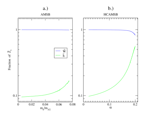
While the lightest neutralino is mainly wino-like in mAMSB and HCAMSB models, it is important phenomenologically to realize that for certain regions of parameter space, the picks up a substantial higgsino component, thus becoming a mixed wino/higgsino particle. This occurs in mAMSB at large values, and in HCAMSB at large values. The situation is shown in Fig. 1 for TeV, and , where we show (the wino component of in the notation of Ref. [1]) and (the higgsino component of ) as a function of a). in mAMSB and b). for HCAMSB. We see indeed that in both these cases, is increasing as the relevant parameter increases.
2.3 Gaugino AMSB
Phenomenologically viable versions of string theory require the stabilization of all moduli fields as well as weak to intermediate scale supersymmetry breaking. Models satisfying these criteria were first developed in the context of type IIB string theory using flux compactifications and non-perturbative effects on Calabi-Yau orientifolds (CYO’s)[36]. The low energy limit of type-IIB string theory after compactification on a CYO is expected to be supergravity (SUGRA).
Two classes of the above models which yield an interesting supersymmetry breaking scenario have been studied:
-
a)
Those with only a single Kähler modulus (SKM models). These are essentially of the KKLT type [37] but with uplift coming from one-loop quantum effects.
-
b)
Large Volume Scenario (LVS)[38] models which require at least two moduli.
In both of these types of models, the moduli fields are stabilized using a combination of fluxes and non-perturbative effects. Additionally, supersymmetry is broken by the moduli fields acquiring non-zero F-terms and interacting gravitationally with the MSSM. For both models, the gauginos acquire mass predominately through the Weyl anomaly while the classical contribution to the scalar masses and trilinear coupling constants are naturally suppressed. Here, we take the limit where scalar and trilinear soft breaking parameters are exactly zero at the GUT scale: , while gaugino masses are of the AMSB form. The parameter space of inoAMSB models is then given by
| (8) |
As shown in Ref. [13], the inoAMSB model solves the problem of tachyonic scalars in AMSB, since now the GUT scale scalar masses vanish. It also solves the problem of charged LSPs which is endemic to no-scale SUGRA or gaugino-mediated SUSY breaking (inoMSB) models, which have but with universal gaugino masses equal to . For inoAMSB models–with scalar masses at the GUT scale– the large GUT-scale gaugino mass pulls all scalar masses to large values, leaving no tachyons and a wino-like neutralino as the lightest MSSM particle.
2.4 Thermally produced wino CDM in AMSB models
The above mAMSB and HCAMSB models have been included into the Isasugra subprogram of the event generator Isajet[39]. In addition, sparticle mass spectra for the inoAMSB model can easily be generated using usual mSUGRA input parameters with , but with non-universal gaugino masses as specified by AMSB models.
After input of mAMSB, HCAMSB or inoAMSB parameters, Isasugra then implements an iterative procedure of solving the MSSM RGEs for the 26 coupled renormalization group equations, taking the weak scale measured gauge couplings and third generation Yukawa couplings as inputs, as well as the above-listed GUT scale SSB terms. Isasugra implements full 2-loop RG running in the scheme, and minimizes the RG-improved 1-loop effective potential at an optimized scale choice [40] to determine the magnitude of and . All physical sparticle masses are computed with complete 1-loop corrections, and 1-loop weak scale threshold corrections are implemented for the , and Yukawa couplings[41]. The off-set of the weak scale boundary conditions due to threshold corrections (which depend on the entire superparticle mass spectrum), necessitates an iterative up-down RG running solution. The resulting superparticle mass spectrum is typically in close accord with other sparticle spectrum generators[42].
Once the weak scale sparticle mass spectrum is known, then sparticle annihilation cross sections may be computed. To evaluate the thermally produced neutralino relic density, we adopt the IsaReD program[43], which is based on CalcHEP[44] to compute the several thousands of neutralino annihilation and co-annihilation Feynman diagrams. Relativistic thermal averaging of the cross section times velocity is performed[45].
As an example, in Fig. 2, we show the thermally produced neutralino relic density versus for all three models: mAMSB, HCAMSB and inoAMSB. We take and . For mAMSB, we also take , and for HCAMSB, we take . On the upper axis, we also indicate the corresponding values of . We see that the relic abundance is typically well below WMAP7-measured levels, until TeV, corresponding to TeV, and TeV: well beyond any conceivable LHC reach. The well-known tiny relic abundance arises due to the large annihilation and also and co-annihilation processes.
3 Dark matter scenarios for AMSB models
3.1 Neutralino production via moduli decay
Shortly after the introduction of AMSB models, Moroi and Randall proposed a solution to the AMSB dark matter problem based on augmented neutralino production via the decays of moduli fields in the early universe[19]. The idea here is that string theory is replete with additional moduli fields: neutral scalar fields with gravitational couplings to matter. In generic supergravity theories, the moduli fields are expected to have masses comparable to . When the Hubble expansion rate becomes comparable to the moduli mass , then an effective potential will turn on, and the moduli field(s) will oscillate about their minima, producing massive excitations, which will then decay to all allowed modes: e.g. gauge boson pairs, higgs boson pairs, gravitino pairs, . The neutralino production rate via moduli decay has been estimated in Ref. [19]. It is noted in Ref. [46] that the abundance– given by
| (9) |
with cm3/sec– yields nearly the measured dark matter abundance for wino-like neutralino annihilation cross sections and TeV.111In inoAMSB models, we expect moduli with SUSY breaking scale masses, , where is the (large) volume of the compactified manifold: in Planck units. In this case, the mechanism would not so easily apply. These authors dub this the “non-thermal WIMP miracle”.
A necessary condition for augmented neutralino production via scalar field decay is that the re-heat temperature of radiation induced by moduli decays is bounded by MeV (in order to sustain Big Bang Nucleosynthesis (BBN) as we know it), and , where is the freeze-out temperature for thermal neutralino production . If exceeds , then the decay-produced neutralinos will thermalize, and the abundance will be given by the thermal calculation as usual.
This “low re-heat” neutralino production mechanism has been investigated extensively by Gondolo and Gelmini[47]. The low re-heat neutralino abundance calculation depends on the input value of and the ratio , where is the average number of neutralinos produced in moduli decay, and is the scalar field mass. They note that theories with an underabundance of thermally produced neutralino CDM with can always be brought into accord with the measured DM abundance for at least one and sometimes two values of .222Ref. [47] also shows that an overabundance of thermally produced neutralino CDM can also be brought into accord with the measured abundance via dilution of the neutralino number density by entropy injection from the field decay. Since this case doesn’t attain in AMSB models (unless GeV), we will neglect it here.
While the low MeV scenario with DM generation via scalar field decay is compelling, we note here that it is also consistent with some baryogenesis mechisms: e.g. Affleck-Dine baryogenesis wherein a large baryon asymmetry is generated early on, only to be diluted to observable levels via moduli decay[48], or a scenario wherein the baryon asymmetry is actually generated by the moduli decay[49].
3.2 Neutralino production via gravitino decay
An alternative possibility for augmenting the production of wino-like neutralinos in AMSB models is via gravitino production and decay in the early universe. While gravitinos would not be in thermal equilibrium during or after re-heat, they still can be produced thermally via radiation off ordinary sparticle scattering reactions in the early universe. The relic density of thermally produced gravitinos as calculated in Ref’s [50, 21] is given by
| (10) |
where and are the gauge couplings and gaugino masses evaluated at scale , and and . Each gravitino ultimately cascade decays down to the wino-like state, so the neutralino relic density is given by
| (11) |
A plot of the value of and which is required to yield from Eq’n 11 is shown in Fig. 3 for mAMSB (), HCAMSB () and inoAMSB using and . The region above the curves would yield too much dark matter, while the region below the curves yields too little.
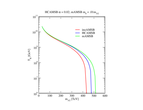
We should consider the curves shown in Fig. 3 as only indicative of the simplest scenario for wino production via gravitino decay. Three other effects can substantially change the above picture from what is presented in Eq. 11.
-
•
On the one hand, if moduli fields exist with mass , then gravitinos can also be produced via moduli production and decay[22]. The exact abundance of these moduli-produced gravitinos is very model dependent, and depends on the moduli and gravitino mass and branching fractions.
-
•
A second case arises if we consider gravitino production via inflaton decay at the end of inflation[23]. This production mechanism depends on unknown properties of the inflaton: e.g. its mass and branching fractions, and the re-heat temperature generated by inflaton decay. These latter quantities are very model dependent.
-
•
Additional entropy production generated via the inflaton, moduli and gravitino decays may also dilute the above relic abundance in Eq. 11.
We will bear in mind that these possibilities permit much lower or much higher values of and than those shown by the contour of Fig. 3.
3.3 Neutralino production via heavy axino decay
A third mechanism for increasing the wino-like relic abundance is presented in Ref. [26], in the context of the PQMSSM. If we adopt the Peccei-Quinn (PQ) solution to the strong problem within the context of supersymmetric models, then it is appropriate to work with the PQ-augmented MSSM, which contains in addition to the usual MSSM states, the axion , the -parity even saxion field , and the spin- -parity odd axino . The axino can serve as the lightest SUSY particle if it is lighter than the lightest -odd MSSM particle. The and have couplings to matter which are suppressed by the value of the PQ breaking scale , usually considered to be in the range GeV[27].
In Ref. [26], it is assumed that , where is the LSP. In the AMSB scenarios considered here, we will assume GeV, so as to avoid overproduction of dark matter via gravitinos. With these low values of , we are also below the axino decoupling temperature , so the axinos are never considered at thermal equilibrium[30]. However, axinos can still be produced thermally via radiation off usual MSSM scattering processes at high temperatures. The calculation of the thermally produced axino abundance, from the hard thermal loop approximation, yields[25]
| (12) |
where is the strong coupling evaluated at and is the model dependent color anomaly of the PQ symmetry, of order 1. Since these axinos are assumed quite heavy, they will decay to or modes, which further decay until the stable LSP state, assumed here to be the neutral wino, is reached.
If the temperature of radiation due to axino decay () exceeds the neutralino freeze-out temperature , then the thermal wino abundance is unaffected by axino decay. If , then the axino decay will add to the neutralino abundance. However, this situation breaks up into two possibilities: a). a case wherein the axinos can dominate the energy density of the universe, wherein extra entropy production from heavy axino decay may dilute the thermal abundance of the wino-like LSPs, and b). a case where they don’t. In addition, if the yield of winos from axino decay is high enough, then additional annihilation of winos after axino decay may occur; this case is handled by explicit solution of the Boltzmann equation for the wino number density. Along with a component of wino-like neutralino CDM, there will of course be some component of vacuum mis-alignment produced axion CDM: thus, in this scenario, we expect a WIMP/axion mixture of CDM.
3.4 Mixed axion/axino CDM in AMSB models
In this case, we again consider the PQMSSM, as in Subsec. 3.3. But now, we consider a light axino with , so that is the stable LSP[24]. Here, the thermally produced wino-like neutralinos will decay via , so we will obtain a very slight dark matter abundance from neutralino decay: , since each thermally produced neutralino gives rise to one non-thermally produced (NTP) axino. We will also produce axinos thermally via Eq’n 12. Finally, we will also produce axion CDM via the vacuum mis-alignment mechanism[51]: (we will take here the initial mis-alignment angle ). The entire CDM abundance is then the sum
| (13) |
In this case, the TP axinos constitute CDM as long as MeV. The NTP axinos constitute warm DM for GeV[52], but since their abundance is tiny, this fact is largely irrelevant. The entire CDM abundance then depends on the parameters , and ; it also depends extremely weakly on , since this is usually small in AMSB models.
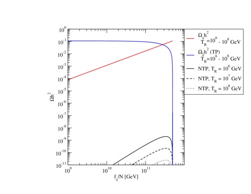
As an example, we plot in Fig. 4 the three components of mixed axion/axino DM abundance from HCAMSB benchmark point 1 in Ref. [35]: , TeV, and . The neutralino thermal DM abundance would be if the was stable. We require instead , and plot the three components of versus , for three values of , and GeV. The value of is determined by the constraint . We see that at low values of , the NTP axino abundance is indeed tiny. Also the axion abundance is tiny since the assumed initial axion field strength is low. The TP axino abundance dominates. As increases, the axion abundance increases, taking an ever greater share of the measured DM abundance. The TP axino abundance drops with increasing , since the effective axino coupling constant is decreasing. Around GeV, the axion abundance becomes dominant. It is in this range that ADMX[53] would stand a good chance of measuring an axion signal using their microwave cavity experiment.
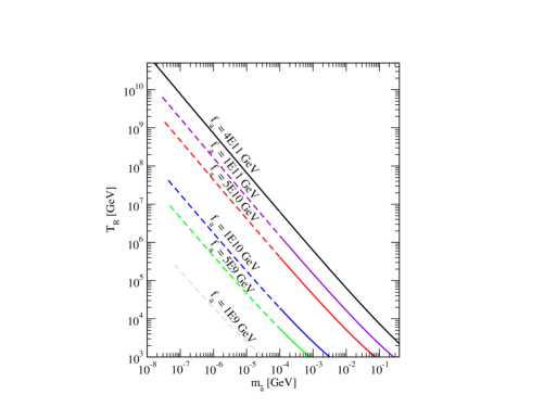
In Fig. 5, we again require for HCAMSB benchmark point 1, but this time plot the value of which is needed versus , for various values of . The plots terminate at high in order to avoid reaching the axion decoupling temperature . Dashed curves indicate regions where over 50% of the DM is warm, instead of cold. Solid curves yield the bulk of DM as being cold.
We see that for very light axino masses, and large values of , the value of easily reaches beyond GeV, while maintaining the bulk of dark matter as cold . Such high values of are good enough to sustain baryogenesis via non-thermal leptogenesis[54], although thermal leptogenesis requires GeV[55]. Since is quite large, we would expect that the dominant portion of DM is composed of relic axions, rather than axinos; as such, detection of the relic axions may be possible at ADMX[53]. While Fig’s 4 and 5 were created for the HCAMSB model, quite similar results are obtained for the mAMSB or inoAMSB models.
4 Direct and indirect detection of wino CDM in AMSB models
For AMSB dark matter cases 1 and 2 above, it is expected that the thermal wino abundance will be supplemented by either moduli or gravitino decay in the early universe, thus increasing the wino abundance into accord with measured values. In these cases, it may be possible to detect relic wino-like WIMPs with either direct or indirect detection experiments[56]. Also, in case 3 above, it is expected that the DM abundance is comprised of an axion/wino mixture. If the wino component of this mixture is substantial, then again direct or indirect WIMP detection may be possible, while if axions are dominant, then a WIMP signal is less likely, but direct detection of relic axions is more likely: in a nearly equal mixture of WIMPs and axions, possibly detection of both could occur! In case 4 above, we would expect no WIMP signals to occur in either direct or indirect detection experiments.
4.1 Direct wino detection rates in AMSB models
Direct detection of WIMPs depends on the WIMP-nucleon scattering cross section, but also on assumptions about the local WIMP density (usually assumed to be ), and the velocity distribution of the relic WIMPs (usually assumed to follow a Maxwellian distribution where km/sec, the sun’s velocity about the galactic center). In our case, where WIMPs are mainly produced non-thermally via moduli, gravitino or axino decay, the original velocity distribution due to decays will be red-shifted away and the current distribution will arise mainly from gravitational infall, as is the case with thermal WIMP production. The direct detection reach plots are usually presented in terms of the WIMP-nucleon scattering cross section. Then, the experimental reach depends on factors like the mass and spin of the nuclear target, and the assumed local WIMP density and velocity profiles.
Direct detection of WIMPs is usually broken down into two components: detection via spin-independent (SI) interactions , and detection via spin-dependent interactions (SD). For SI interactions, it may be best to use heavy target nuclei, since the SI nucleon-WIMP interactions sum coherently over the nuclear mass. For the SI WIMP-nucleon cross section, we use the Isatools subroutine IsaReS[57].
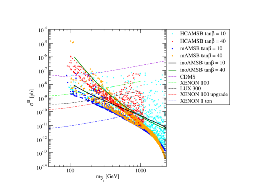
Our results for SI direct detection of wino-WIMPs is shown in Fig. 6, in the plane. Here, we scan over for all models, and (for mAMSB) and (for HCAMSB). We show results for and 40, while taking . The inoAMSB results occur as lines, since there is no or dependence. We keep only solutions that obey the LEP2 limit on a wino-like chargino: GeV[58].
Several crucial features emerge from the plot. First, we note that for a given value of , the value of is bounded from below, unlike the case of the mSUGRA model. That means that wino-WIMP dark matter can be either detected or excluded for a given value. Second, we note that the cross section values generally fall in the range that is detectable at present or future DD experiments. The purple contour, for instance, exhibits the CDMS reach based on 2004-2009 data, and already excludes some points, especially those at large . We also show the reach of Xenon-100, LUX, Xenon-100 upgrade, and Xenon 1 ton[59]. These experiments should be able to either discover or exclude AMSB models with values below and 500 GeV respectively. These WIMP masses correspond to values of and 3850 GeV, respectively! The latter reach far exceeds the 100 fb-1 of integrated luminosity reach of LHC for .333In Ref. [35], the 100 fb-1 reach of LHC for HCAMSB is found to be TeV. In Ref. [13], the 100 fb-1 reach of LHC for inoAMSB was found to be TeV. For inoAMSB models, where the minimal value of exceeds that of mAMSB or HCAMSB for a given value, the Xenon 1 ton reach is to GeV, corresponding to a reach in of 6200 GeV!
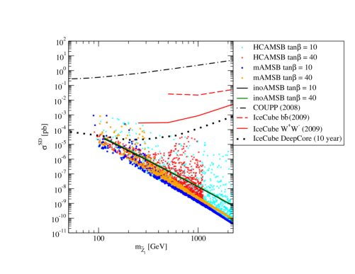
In Fig. 7, we show the SD direct detection cross section versus for mAMSB, HCAMSB and inoAMSB models with and 40. We also show a recent limit on this cross section from the COUPP experiment, which is above the theory expectation by two orders of magnitude. We also show two limits from IceCube in 2009, which do approach the theory region, but only for rather large values of . The IceCube SD reach is quite significant, because the rate for WIMP annihilation in the core of the sun mainly depends on the sun’s ability to sweep up neutralinos as it passes along its orbit. The target here is the solar hydrogen, where the SD cross section usually dominates the SI one, since the atomic mass is minimal (an enhancement by number of nucleons per nucleus is usually necessary to make the SI cross section competetive with the SD one). Since IceCube is mainly sensitive to very high energy muons with GeV, it can access mainly higher values of . The IceCube DeepCore reach is also shown. The DeepCore project will allow IceCube to access much lower energy muons, and thus make it more useful for generic WIMP searches. While DeepCore will access a portion of parameter space, it will not reach the lower limit on SD cross sections as predicted by AMSB models.
4.2 Indirect wino detection rates in mAMSB
Next, we present rates for indirect detection (ID) of wino-like DM via neutrino telescopes, and via detection of gamma rays and anti-matter from WIMP annihilation in the galactic halo. The ID detection rates depend (quadratically[60]) on the assumed galactic DM density (halo) profile. We will show results using two profiles: isothermal and Navarro-Frenk-White (NFW)[61] (see e.g. [62] for plots of several recent halo profiles). Most halo models are in near accord at the earth’s position at kpc from the galactic center. However, predictions for the DM density near the galactic center differ wildly, which translates to large uncertainties for DM annihilation rates near the galactic core. The corresponding uncertainty will be smaller for anti-protons, and smaller still for positrons; since these particles gradually lose energy while propagating through the galaxy, they can reach us only from limited distances over which the halo density is relatively well-known. Possible clumping of DM yields an additional source of uncertainty in ID detection rates.
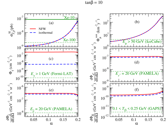
In Fig. 8a.), we show for comparison the SI direct detection scattering cross section versus in the mAMSB model for TeV and . For these parameters, the wino-like neutralino has mass GeV. We also indicate an approximate reach of Xenon-10 and Xenon-100. While the SI direct detection cross section is just below Xenon-100 reach for low , as increases, the value of drops, much as it does in mSUGRA as we approach the focus point region. For large , the becomes mixed wino-higgsino, and its direct detection cross section increases into the range which is accessible to Xenon-100.
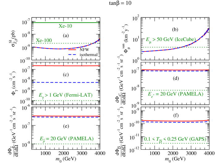
In Fig. 8b.), we show the flux of muons from conversions at earth coming from neutralino annihilation to SM particles within the solar core. Here, we use the Isajet/DarkSUSY interface for our calculations[63], and require GeV. The predicted rate depends, in this case, mainly on the sun’s ability to sweep up and capture neutralinos, which depends mainly on the spin-dependent neutralino-nucleon scattering cross section (since in this case, the neutralinos mainly scatter from solar Hydrogen, and there is no mass number enhancement), which is mostly sensitive to exchange. The rates are again low for low with wino-like neutralinos. They nearly reach the IceCube detectability level at large where the neutralinos, while remaining mainly wino-like, have picked up an increasing higgsino component, so that the neutralino couplings to become large.
In Fig. 8c.), we show the expected flux of gamma rays with GeV, as required for the Fermi Gamma-ray Space Telescope (FGST), arising from DM annihilations in the galactic core. In this case, we see a signal rate which is flat with respect to . Here, the rate depends mainly on the annihilation cross section, which occurs via chargino exchange; since the s remain mainly wino-like, and the chargino mass hardly varies, the annihilation rate hardly varies with . The predictions for two halo profiles differ by over an order of magnitude, reflecting the large uncertainty in our knowledge of the DM density at the center of our Galaxy. Both projections are above the approximate reach of the FGST.
In Fig. 8d.)-f.), we show the expected flux of positrons , antiprotons and antideuterons from neutralino halo annihilations. Each of these frames show detectable rates by Pamela[64] (for s and s) and by GAPS[65] (for anti-deuterons). These elevated IDD rates (compared to mSUGRA[66] for similar values) for anti-matter detection reflect the elevated rate for the annihilation into cross section. The halo model uncertainty for anti-matter detection is much smaller than in the -ray case, since for charged particle detection, it is necessary that the anti-matter is generated relatively close to earth, where the DM density profile is much better known.
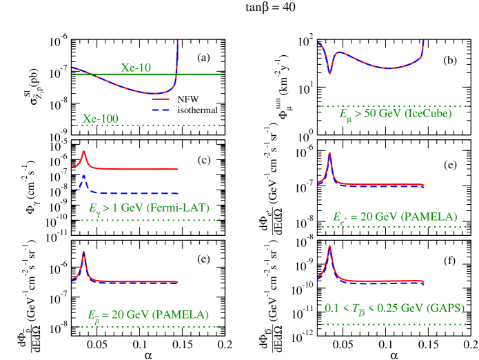
In Fig. 9, we show rates for direct and indirect detection of wino-like WIMPs in mAMSB versus with TeV, and . The SI direct detection rate shown in Fig. 9a.) shows a notable enhancement at low , and the usual enhancement at large due to the increasing higgsino component of . The low enhancement arises because the mass of the heavy Higgs scalar has dropped with increasing , and is now quite light: GeV for GeV (compared to GeV for the same with . The loop diagram via exchange is enhanced, resulting in a huge direct detection cross section. This range of is already excluded by DD WIMP searches!
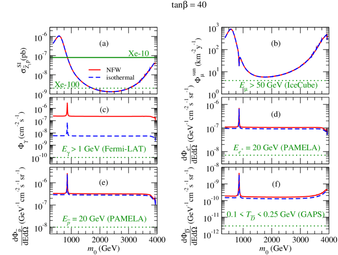
In Fig. 9b.), we show the muon flux from mAMSB models versus for TeV and . In this case, we again see a huge enhancement at low . While normally the SD cross section dominates the solar accretion rate for WIMPs, in this case, the 3 order-of-magnitude increase in SI cross section shown in frame a.) contributes and greatly increases the solar capture rate, and hence the muon flux from the sun. Of course, this region would already be excluded by present DD limits. We also see a curious “anti-resonance” effect in around GeV. In this case, , and neutralino annihilation is enhanced by the resonance. Normally, for AMSB models, ( or ) is the dominant annihilation mechanism. But on the Higgs resonance, instead dominates. The energy distribution of neutrinos from decay is far softer than that from or decay, leading to conversions to lower energy muons. Since we require GeV for IceCube, fewer muons are detected, and hence the anti-resonance effect. At large and , the muon flux is again enhanced by the increased WIMP scattering rate via its increasing higgsino component.
In Fig. 9c-f.), we see the flux of gamma rays and anti-matter versus at large . Here, the rate versus is again flat, reflecting the usually constant annihilation rate into vector bosons. The exception occurs at GeV, where annihilation through the -resonance enhances the halo annihilation rate[66]. At large and , the and detection rates drop. This is due to the changing final state from annihilation: at low it is mainly to vector bosons, leading to a hard and distribution. At large , annihilations to increase and become prominent, but the energy distribution of and softens, and since we require GeV, the detection rate drops. In frame f.), showing the rate, the rate actually increases at large , since here we already require quite low energy s for detection, and the distribution only reflects the increased annihilation rate.
4.3 Indirect wino detection rates in HCAMSB
In this subsection, we present wino-like WIMP DD and ID rates in the HCAMSB model for TeV, versus varying . As shown in Ref. [35], a low value of corresponds to pure anomaly-mediation, while large gives an increasing mass to the hypercharge gaugino at the GUT scale. The large value of pulls sparticle masses to larger values via RG evolution, with the pull increasing in accord with the matter state’s hypercharge quantum number: thus– at large – we expect relatively heavy states, but comparatively light and states. In fact, the RGE effect– coupled with the large -quark Yukawa coupling[1]– leads to relatively light, and dominantly left-, top squark states at large . For very high values of , the value of diminishes until radiative EWSB no longer occurs (much as in the focus point region of mSUGRA).
In Fig. 10a.), we show the SI neutralino direct detection rate versus for . The cross section is of order pb at low , consistent with pure wino-like neutralinos. As increases, the increasing sparticle masses feed into , diminishing the term and leading to a lessened downward push by the top Yukawa coupling. Since at the weak scale, the term is also diminished, leading to an increasing higgsino component of . The increased higgsino component yields an enhanced via Higgs exchange at large .
In Fig. 10b.), we plot the muon flux in the HCAMSB model vs. . The muon flux is quite small at low , but at high , the increasing higgsino component of leads to an increased via -exchange. In Fig’s 10c-f.), we plot the -ray, , and fluxes versus . In these cases, the rates are large due to the large annihilation cross section and is relatively flat with . At the largest values, annihilation to states is enhanced, leading to diminished rates for and (due to softened energy distributions) but to a slightly increased rate for s.
In Fig. 11, we show the same rates vs. in the HCAMSB model, except now for . The SI direct detection rate in Fig. 11a.) is enhanced relative to the case due to the much lighter Higgs mass and the increased -quark Yukawa coupling. The rate diminishes as increases due to increasing squark and Higgs masses, until very high is reached, and the rate is enhanced by the growing higgsino component of . The parameter space terminates above due to lack of REWSB.
In Fig. 11b.), we see that the muon flux due to solar core annihilations is also enhanced. In this case, the increase is again due to the large enhancement in SI scattering cross section, which feeds into the solar accretion rate. As in Fig. 9b.), we find an anti-resonance dip at the value where , and WIMP annihilations occur instead mainly into rather than states. Fig’s 11c-f.) show the halo annihilation rates for HCAMSB at . These rates are generally flat with changing , and do not suffer an increase compared with low results, since still dominates the annihilation rate. The exception occurs at , where , and halo annihilation is enhanced by the pseudoscalar Higgs resonance.
4.4 Indirect detection rates vs. for mAMSB, HCAMSB and inoAMSB
In Fig. 12, we show direct and indirect wino DM detection rates versus for and . For mAMSB, we take TeV, while for HCAMSB, we take . The associated mass spectra versus can be found in Ref. [35] for mAMSB and HCAMSB, and in Ref. [13] for the inoAMSB model. Spectra for all three models are shown in Table 1 of Ref. [13] for the case of TeV.
In Fig. 12a.), the SI direct detection cross section is shown for all three models. In this case, we see for a given value of , the inoAMSB model gives the highest cross section, while mAMSB gives the lowest. The larger inoAMSB cross section is due in part because inoAMSB models have a smaller value for a given value of , and so SI scattering via Higgs exchange (which involves a product of higgsino and gaugino components) is enhanced.
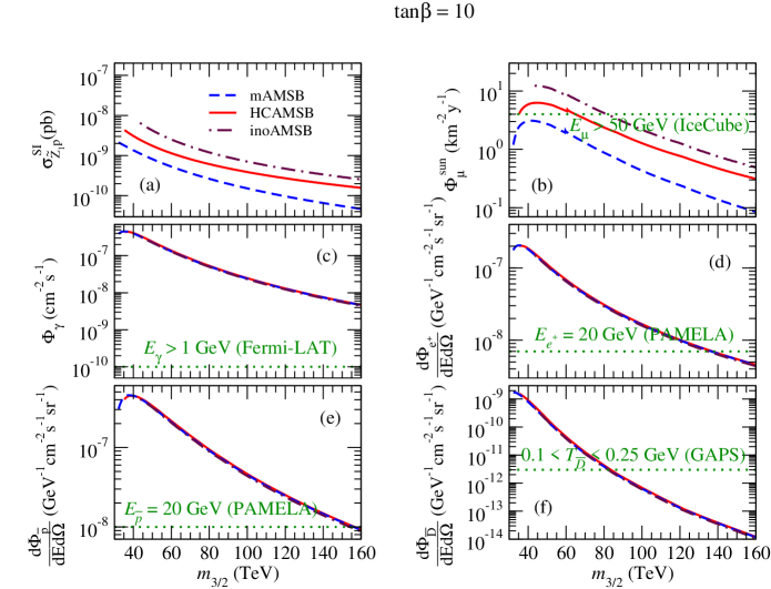
In Fig. 12b.), we show the relative rates for indirect wino detection due to WIMP annihilation into states in the solar core, with subsequent muon detection from conversions in Antarctic ice, as might be seen by IceCube. We require GeV. The muon flux is mainly related to the spin-dependent direct detection rate, which enters the sun’s ability to capture WIMPs. Here again, inoAMSB yields the highest rates, and mAMSB the lowest. This follows the relative values of in the three models: low in inoAMSB leads to a larger higgsino component of , and an increased SD scattering rate via exchange. A rough reach of the IceCube detector is shown, and indicates that the low portion of parameter space of inoAMSB and HCAMSB may be accessible to searches.
In Fig. 12c-f.), we show the ID rates for detection of , s, s and s, for the energy ranges indicated on the plots. All these plots adopt the NFW halo profile. In all these cases, all three models yield almost exactly the same detection rates for a given value of . This is due to the dominance of halo annihilations, which mainly depend on the gaugino component of , which is nearly all wino-like. The rough reach of Fermi-LAT, Pamela and GAPS is shown for reference. The high rates for wino halo annihilations should yield observable signals. As mentioned previously, Kane et al. promote wino-like WIMPs as a source of the Pamela anomaly[31]. In this case, a large signal should be seen as well, although the Pamela rate seems to agree with SM background projections.
In Fig. 13, we show direct and indirect wino detection rates versus as in Fig. 12, except now for a large value of . In frame a.), we see that the SI direct detection rates are all elevated with respect to the case. The well-known large enhancement[67, 68] occurs due to enhanced Higgs exchange contributions, where now the value of is lower and the -quark Yukawa coupling is larger. For low , the inoAMSB model has the smallest value of and the lowest value of for a given value, and thus the highest value of . As increases, the value of increases for inoAMSB and HCAMSB, while it actually decreases for mAMSB. Thus, for TeV, the mAMSB model yields the highest value of .
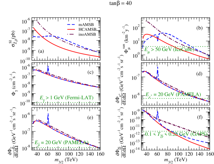
In Fig. 13b.), we show the muon flux for IceCube due to wino annihilation in the solar core. Here again, the rates are elevated compared to the case. The inoAMSB model yields the highest flux at low , since it has the lowest value, and the highest higgsino component, which enters into the exchange diagram for scattering. At TeV in the mAMSB model, we obtain , and the solar core annihilations mainly proceed to states instead of , which diminishes the muon energy distribution and hence the detection rate for s with GeV. At higher values, the resonance is passed, and annihilation once again proceeds dominantly into . For high , the mAMSB model yields the highest muon flux, due to its elevated value of .
In Fig. 13c-f.), we find relatively little change in halo annihilation rates due to an increase in , since the annihilations mainly proceed via , which depends mainly on gauge couplings. The exception occurs in the mAMSB model, where we do get the resonance enhancement of halo annihilations when . We also obtain some enhancement of the detection rate for inoAMSB and mAMSB at large because in these cases the annihilation rate, which does receive enhancement, contributes to the detection of rather low energy s.
5 Discussion and conclusions
In this paper, we have investigated aspects of cold dark matter in three models of anomaly mediation: mAMSB, HCAMSB and inoAMSB. Typically, each gives rise to a wino-like lightest neutralino, unless very high values of (for mAMSB) or (for HCAMSB) are used, in which case the becomes a mixed wino-higgsino state. In this class of models with a wino-like , the thermal abundance of neutralino CDM is well below measured values, unless GeV. We discuss four ways to reconcile the predicted abundance of CDM with experiment:
-
1.
enhanced neutralino production via scalar field (e.g. moduli) decay,
-
2.
enhanced neutralino production via gravitino decay, where gravitinos may arise thermally, or by moduli or inflaton decay,
-
3.
enhanced neutralino production via heavy axino decay, and
-
4.
neutralino decay to axinos, where the bulk of CDM comes from a mixture of vacuum mis-alignment produced axions and thermally produced axinos.
Cases 1 and 2 should lead to a situation where all of CDM is comprised of wino-like WIMPs; they will be very hard, perhaps impossible, to tell apart. Case 3 would contain a mixture of axion and wino-like WIMP CDM. It is a scenario where it is possible that both a WIMP and an axion could be detected. Case 4 predicts no direct or indirect detection of WIMPs, but a possible detection of relic axions. It is important to note that more than one of these mechanisms may occur at once: for instance, we may gain additional neutralino production in the early universe from moduli, gravitino and axino decay all together.
In Sec. 4, we presented rates for direct and indirect detection of relic wino-like WIMPs. The SI direct detection cross sections are bounded from below. Ultimately, ton-scale noble liquid or SuperCDMS experiments should probe out to GeV, which would exceed the 100 fb-1 reach of LHC; a non-observation of signal would put enormous stress on AMSB-like models as new physics. We also evaluated SD direct detection: current experiments have little reach for AMSB-like models, although IceCube DeepCore and possibly COUPP upgrades may probe more deeply.
We also presented indirect WIMP detection rates for all three AMSB models. The IceCube experiment has some reach for WIMPs from AMSB models, especially at high or when the picks up a higgsino component. We noted an interesting inverse resonance effect in the muon flux detection rate, caused by transition from solar core annihilations to states, to annihilations to mainly states. The detection of s, s, s and s are all elevated in AMSB-like models compared to mSUGRA, due to the high rate for annihilation in the galactic halo. The results do depend on the assumed halo profile, especially for -ray detection in the direction of the galactic core. Generally, if a signal is seen in the channel, then one ought to be seen in the channel, and ultimately in the , (if/when GAPS flies) or direct detection channel. In addition, a sparticle production signal should ultimately be seen at LHC, at least for GeV, once 100 fb-1 of integrated luminosity is accrued.
As a final remark, we note here that the dark matter detection signals all provide complementary information to that which will be provided by the CERN LHC. At LHC, each model– mAMSB, HCAMSB and inoAMSB– will provide a rich assortment of gluino and squark cascade decay signals which will include multi-jet plus multi-lepton plus missing events. In all cases, the wino-like lightest neutralino state will be signaled by the well-known presence of highly ionizing tracks (HITs) from quasi-stable charginos with track length of order cms, before they decay to soft pions plus a . It is noted in Ref’s [35] and [13] that the three models should be distinguishable at LHC by the differing opposite-sign/same flavor dilepton invariant mass distributions. In the case of mAMSB, with , we expect a single mass edge from decay. In HCAMSB, the sleptons are rather heavy, and instead occurs at a large rate, leading to a bump in , upon a continuum distribution. In inoAMSB, with , but with and split in mass (due to different quantum numbers), a characteristic double mass edge is expected in the invariant mass distribution.
Acknowledgments
We thank Shanta de Alwis for comments on the manuscript. This work was supported in part by the U.S. Department of Energy.
References
- [1] H. Baer and X. Tata, Weak Scale Supersymmetry: From Superfields to Scattering Events, (Cambridge University Press, 2006)
- [2] S. Dimopoulos, S. Raby and F. Wilczek, Phys. Rev. D 24 (1981) 1681; S. Dimopoulos and H. Georgi, Nucl. Phys. B 193 (1981) 150; L. Ibanez and G. Ross, Phys. Lett. B 105 (1981) 439; N. Sakai, Z. Phys. C11 (1981) 153; M. Einhorn and D. R. T. Jones, Nucl. Phys. B 196 (1982) 475; W. Marciano and G. Senjanovic, Phys. Rev. D 25 (1982) 3092.
- [3] U. Amaldi, W. de Boer and H. Furstenau, Phys. Lett. B 260 (1991) 447; J. Ellis, S. Kelley and D. V. Nanopoulos, Phys. Lett. B 260 (1991) 131; P. Langacker and Luo, Phys. Rev. D 44 (1991) 817.
- [4] D. Freedman, S. Ferrara and P. van Nieuwenhuizen, Phys. Rev. D 13 (1976) 3214; S. Deser and B. Zumino, Phys. Lett. B 62 (1976) 335; S. Ferrara, D. Freedman, P. van Nieuwenhuizen, P. Breitenlohner, G. Gliozzi and J. Scherk, Phys. Rev. D 15 (1977) 1013; E. Cremmer, S. Ferrara, L. Girardello and A. van Proeyen, Nucl. Phys. B 212 (1983) 413
- [5] M. Dine, W. Fischler and M. Srednicki, Nucl. Phys. B 189 (1981) 575; S. Dimopoulos and S. Raby, Nucl. Phys. B 192 (1982) 353; M. Dine and W. Fischler, Phys. Lett. B 110 (1982) 227 and Nucl. Phys. B 204 (1982) 346; C. Nappi and B. Ovrut, Phys. Lett. B 113 (1982) 175; L. Alvarez-Gaume, M. Claudson and M. Wise, Nucl. Phys. B 207 (1982) 96; S. Dimopoulos and S. Raby, Nucl. Phys. B 219 (1983) 479; M. Dine, A. Nelson, Y. Nir and Y. Shirman, Phys. Rev. D 53 (1996) 2658; for a review, see G. Giudice and R. Rattazzi, Phys. Rept. 322 (1999) 419.
- [6] L. Randall and R. Sundrum, Nucl. Phys. B 557 (1999) 79.
- [7] G. Giudice, M. Luty, H. Murayama and R. Rattazzi, J. High Energy Phys. 12 (1998) 027.
- [8] For recent discussion, see M. Dine and N. Seiberg, J. High Energy Phys. 0703 (2007) 040; S. de Alwis, Phys. Rev. D 77 (2008) 105020.
- [9] I. Jack and D. R. T. Jones, Phys. Lett. B 465 (1999) 148.
- [10] S. Weinberg, Phys. Rev. Lett. 48 (1982) 1303; R. H. Cyburt, J. Ellis, B. D. Fields and K. A. Olive, Phys. Rev. D 67 (2003) 103521; K. Jedamzik, Phys. Rev. D 70 (2004) 063524; M. Kawasaki, K. Kohri and T. Moroi, Phys. Lett. B 625 (2005) 7.
- [11] M. Kawasaki, K. Kohri and T. Moroi, Phys. Rev. D 71 (2005) 083502.
- [12] R. Dermisek, H. Verlinde and L-T. Wang, Phys. Rev. Lett. 100 (2008) 131804.
- [13] H. Baer, S. de Alwis, K. Givens, S. Rajagopalan and H. Summy, J. High Energy Phys. 1005 (2010) 069.
- [14] S. P. de Alwis, J. High Energy Phys. 1003 (2010) 078.
- [15] J. R. Ellis, C. Kounnas and D. V. Nanopoulos, Nucl. Phys. B 247 (1984) 373; J. R. Ellis, A. B. Lahanas, D. V. Nanopoulos and K. Tamvakis, Phys. Lett. B 134 (1984) 429; G. A. Diamandis, J. R. Ellis, A. B. Lahanas and D. V. Nanopoulos, Phys. Lett. B 173 (1986) 303; For a review, see A. Lahanas and D. V. Nanopoulos, Phys. Rept. 145 (1987) 1.
- [16] D. E. Kaplan, G. D. Kribs and M. Schmaltz, Phys. Rev. D 62 (2000) 035010; Z. Chacko, M. A. Luty, A. E. Nelson and E. Ponton, J. High Energy Phys. 01 (2000) 003.
- [17] H. C. Cheng, B. Dobrescu and K. Matchev, Nucl. Phys. B 543 (1999) 47.
- [18] E. Komatsu et al. (WMAP collaboration), arXiv:1001.4538 (2010).
- [19] T. Moroi and L. Randall, Nucl. Phys. B 570 (2000) 455.
- [20] M. Bolz, A. Brandenburg and W. Buckmuller, Nucl. Phys. B 606 (2001) 518.
- [21] J. Pradler and F. Steffen, Phys. Rev. D 75 (2007) 023509.
- [22] K. Kohri, M. Yamaguchi and J. Yokoyama, Phys. Rev. D 72 (2005) 083510; T. Asaka, S. Nakamura and M. Yamaguchi, Phys. Rev. D 74 (2006) 023520.
- [23] M. Endo, F. Takahashi and T. T. Yanagida, Phys. Rev. D 76 (2007) 083509.
- [24] L. Covi, J. E. Kim and L. Roszkowski, Phys. Rev. Lett. 82 (1999) 4180; L. Covi, H. B. Kim, J. E. Kim and L. Roszkowski, J. High Energy Phys. 0105 (2001) 033.
- [25] A. Brandenburg and F. Steffen, JCAP0408 (2004) 008.
- [26] K.-Y. Choi, J. E. Kim, H. M. Lee and O. Seto, Phys. Rev. D 77 (2008) 123501.
- [27] For a recent review, see P. Sikivie, hep-ph/0509198; M. Turner, Phys. Rept. 197 (1990) 67; J. E. Kim and G. Carosi, arXiv:0807.3125 (2008).
- [28] H. Baer and H. Summy, Phys. Lett. B 666 (2008) 5.
- [29] H. Baer, A. Box and H. Summy, J. High Energy Phys. 0908 (2009) 080.
- [30] K. Rajagopal, M. Turner and F. Wilczek, Nucl. Phys. B 358 (1991) 447; for recent reviews, see L. Covi and J. E. Kim, arXiv:0902.0769 and F. Steffen, Eur. Phys. J. C 59 (2009) 557.
- [31] P. Grajek, G. Kane, D. Phalen, A. Pierce and S. Watson, Phys. Rev. D 79 (2009) 043506; G. Kane, R. Lu and S. Watson, Phys. Lett. B 681 (2009) 151. D. Feldman, G. Kane, R. Lu and B. Nelson, Phys. Lett. B 687 (2010) 363.
- [32] T. Gherghetta, G. Giudice and J. Wells, Nucl. Phys. B 559 (1999) 27; J. L. Feng, T. Moroi, L. Randall, M. Strassler and S. Su, Phys. Rev. Lett. 83 (1999) 1731; J. L. Feng and T. Moroi, Phys. Rev. D 61 (2000) 095004; F. Paige and J. Wells, hep-ph/0001249; A. Datta and K. Huitu, Phys. Rev. D 67 (2003) 115006; S. Asai, T. Moroi, K. Nishihara and T. T. Yanagida, Phys. Lett. B 653 (2007) 81; S. Asai, T. Moroi and T. T. Yanagida, Phys. Lett. B 664 (2008) 185; H. Baer, J. K. Mizukoshi and X. Tata, Phys. Lett. B 488 (2000) 367; A. J. Barr, C. Lester, M. Parker, B. Allanach and P. Richardson, J. High Energy Phys. 0303 (2003) 045.
- [33] S. Kachru, L. McAllister and R. Sundrum, J. High Energy Phys. 0710 (2007) 013.
- [34] H. Verlinde, L-T. Wang, M. Wijnholt and I. Yavin, J. High Energy Phys. 0802 (2008) 082; M. Buican, D. Malyshev, D. R. Morrison, H. Verlinde and M. Wijnholt, J. High Energy Phys. 0701 (2007) 107.
- [35] H. Baer, R. Dermisek, S. Rajagopalan and H. Summy, J. High Energy Phys. 0910 (2009) 078.
- [36] M. R. Douglas and S. Kachru, Rev. Mod. Phys. 79, 733 (2007) [arXiv:hep-th/0610102].
- [37] S. Kachru, R. Kallosh, A. Linde and S. Trivedi, Phys. Rev. D 68 (2003) 046005.
- [38] V. Balasubramanian, P. Berglund, J. P. Conlon and F. Quevedo, J. High Energy Phys. 03 (2005) 007.
- [39] F. Paige, S. Protopopescu, H. Baer and X. Tata, hep-ph/0312045.
- [40] H. E. Haber, R. Hempfling and A. Hoang, Z. Phys. C75 (1997) 539.
- [41] D. Pierce, J. Bagger, K. Matchev and R. Zhang, Nucl. Phys. B 491 (1997) 3.
- [42] G. Belanger, S. Kraml and A. Pukhov, Phys. Rev. D 72 (2005) 015003.
- [43] IsaRED, by H. Baer, C. Balazs and A. Belyaev, J. High Energy Phys. 0203 (2002) 042.
- [44] CompHEP v.33.23, by A. Pukhov et al., hep-ph/9908288 (1999).
- [45] P. Gondolo and G. Gelmini, Nucl. Phys. B360, 145 (1991); J. Edsjö and P. Gondolo, Phys. Rev. D56, 1879 (1997).
- [46] B. Acharya, G. Kane, S. Watson and P. Kumar, Phys. Rev. D 80 (2009) 083529.
- [47] G. Gelmini and P. Gondolo, Phys. Rev. D 74 (2006) 023510; G. Gelmini, P. Gondolo, A. Soldatenko and C. Yaguna, Phys. Rev. D 74 (2006) 083514; G. Gelmini, P. Gondolo, A. Soldatenko and C. Yaguna, Phys. Rev. D 76 (2007) 015010.
- [48] M. Kawasaki and K. Hakayama, Phys. Rev. D 76 (2007) 043502.
- [49] R. Kitano, H. Murayama and M. Ratz, Phys. Lett. B 669 (2008) 145.
- [50] M. Bolz, A. Brandenburg and W. Buchmuller, Nucl. Phys. B 606 (2001) 518
- [51] L. F. Abbott and P. Sikivie, Phys. Lett. B 120 (1983) 133; J. Preskill, M. Wise and F. Wilczek, Phys. Lett. B 120 (1983) 127; M. Dine and W. Fischler, Phys. Lett. B 120 (1983) 137; M. Turner, Phys. Rev. D 33 (1986) 889; L. Visinelli and P. Gondolo, Phys. Rev. D 80 (2009) 035024.
- [52] K. Jedamzik, M. LeMoine and G. Moultaka, JCAP0607 (2006) 010.
- [53] L. Duffy et al., Phys. Rev. Lett. 95 (2005) 091304 and Phys. Rev. D 74 (2006) 012006; for a review, see S. Asztalos, L. Rosenberg, K. van Bibber, P. Sikivie and K. Zioutas, Ann. Rev. Nucl. Part. Sci.56 (2006) 293.
- [54] G. Lazarides and Q. Shafi, Phys. Lett. B 258 (1991) 305; K. Kumekawa, T. Moroi and T. Yanagida, Prog. Theor. Phys. 92 (1994) 437; T. Asaka, K. Hamaguchi, M. Kawasaki and T. Yanagida, Phys. Lett. B 464 (1999) 12.
- [55] W. Buchmüller, P. Di Bari and M. Plumacher, Nucl. Phys. B 643 (2002) 367 and Erratum-ibid,B793 (2008) 362; Annal. Phys. 315 (2005) 305 and New Jou. Phys.6 (2004) 105.
- [56] P. Grajek, G. Kane, D. Phalen, A. Pierce and S. Watson, arXiv:0807.1508; P. Ullio, J. High Energy Phys. 0106 (2001) 053.
- [57] H. Baer, C. Balazs, A. Belyaev and J. O’Farrill, JCAP 0309, (2003) 007.
- [58] LEPSUSYWG, note LEPSUSYWG/02-04.1.
- [59] See http://dmtools.berkeley.edu/limitplots/, maintained by R. Gaitskell and J. Filippini.
- [60] For reviews, see e.g. G. Jungman, M. Kamionkowski and K. Griest,Phys. Rept. 267 (1996) 195; A. Lahanas, N. Mavromatos and D. Nanopoulos, Int. J. Mod. Phys. D 12 (2003) 1529; M. Drees, hep-ph/0410113; K. Olive, “Tasi Lectures on Astroparticle Physics”, astro-ph/0503065; G. Bertone, D. Hooper and J. Silk, Phys. Rept. 405 (2005) 279. For a recent review of axion/axino dark matter, see F. Steffen, arXiv:0811.3347 (2008).
- [61] J. Navarro, C. S. Frenk and S. D. M. White, Astrophys. J. 462 (1996) 563.
- [62] H. Baer, E. K. Park and X. Tata, New Jou. Phys.11 (105024) 2009.
- [63] P. Gondolo, J. Edsjo, P. Ullio, L. Bergstrom, M. Schelke and E. A. Baltz, JCAP 0407 (2004) 008; for a review, see F. Boudjema, J. Edsjo and P. Gondolo, arXiv:1003.4748.
- [64] M. Pearce (Pamela Collaboration), Nucl. Phys. 113 (Proc. Suppl.) (2002) 314.
- [65] K. Mori, C. J. Hailey, E. A. Baltz, W. W. Craig, M. Kamionkowski, W. T. Serber and P. Ullio, Astrophys. J. 566 (2002) 604; C. J. Hailey et al., JCAP 0601 (2006) 007; H. Baer and S. Profumo, JCAP 0512 (2005) 008.
- [66] H. Baer and J. O’Farrill, JCAP 0404 (2004) 005; H. Baer, A. Belyaev, T. Krupovnickas and J. O’Farrill, JCAP 0408 (2004) 005.
- [67] M. Drees and M. Nojiri, Phys. Rev. D 47 (1993) 376;
- [68] H. Baer and M. Brhlik, Phys. Rev. D 57 (1998) 567