IPPP/10/31 DCPT/10/62 TUM–HEP–756/10


Theoretical and Phenomenological Constraints on
Form Factors for Radiative and Semi-Leptonic B𝐵B-Meson Decays

Aoife Bharucha***a.k.m.bharucha@durham.ac.uk,1, Thorsten Feldmannthorsten.feldmann@ph.tum.de,2, Michael Wickmichael.wick@ph.tum.de,2
1 IPPP, Department of Physics, University of Durham, Durham DH1 3LE, UK

2
Physik-Department, Technische Universität München, D-85748 Garching, Germany


Abstract
We study transition form factors for radiative and rare semi-leptonic B𝐵B-meson decays into light pseudoscalar or vector mesons, combining theoretical constraints and phenomenological information from Lattice QCD, light-cone sum rules, and dispersive bounds. We pay particular attention to form factor parameterisations which are based on the so-called series expansion, and study the related systematic uncertainties on a quantitative level. In this context, we also provide the NLO corrections to the correlation function between two flavour-changing tensor currents, which enters the unitarity constraints for the coefficients in the series expansion.

1 Introduction

At the upcoming LHC experiments (notably LHCb), exclusive B𝐵B-meson decays will play one of the major roles for precision tests of the flavour sector in the Standard Model (SM) and its possible New Physics (NP) extensions [1, 2]. In order to extract information about the underlying short-distance flavour transitions, hadronic matrix elements will be required as theoretical input, and the precision to which they can be predicted will be essential for the success of the flavour program at LHCb. The most prominent example are transition form factors (FFs) for B𝐵B-meson decays into light mesons, which will be the subject of this work. Being non-perturbative hadronic quantities, the theoretical calculation of FFs requires techniques such as Lattice QCD (see e.g. [3, 4, 5, 6, 7]) or QCD sum rules on the light cone (LCSR, see e.g. [8, 9], and [10] and references therein). The two methods are complementary with respect to the momentum transfer q2superscript𝑞2q^{2} between the initial and final-state mesons: In Lattice QCD, results are more easily obtainable at high values of q2superscript𝑞2q^{2}, as discretisation effects can only be controlled for small momenta of the final state in units of the Lattice spacing. This is in contrast to the LCSR method, which involves an expansion in inverse powers of the energy of the light daughter meson that is valid for low values of q2superscript𝑞2q^{2}.

Different FF parameterisations, which can be used to interpolate between the results for small and large momentum transfer, have been suggested in the literature; a good review can be found in [6]. These include simple pole-type parameterisations, like the Bećirević–Kaidalov (BK) approach [11], or variants like the Ball–Zwicky (BZ) parametrisation [8]. Another representation is found from the Omnes solution to the dispersion relation, see the discussion in [12, 13]. In this paper, we will make use of the so-called Series Expansion (SE), which was advocated in Refs. [14, 15, 16, 17, 18]. Here, one can make use of dispersive bounds to obtain additional theoretical constraints on the expansion coefficients. A simplified version of the SE (SSE) was recently suggested in [13]. The aim of this work is to use the SE/SSE to describe the transition FFs on the basis of recent Lattice and LCSR results, including a detailed analysis of systematic errors. We will focus in particular on the FFs entering BVγ𝐵𝑉𝛾B\to V\gamma, BL+𝐵𝐿superscriptsuperscriptB\to L\,\ell^{+}\ell^{-}, BLνν¯𝐵𝐿𝜈¯𝜈B\to L\nu\bar{\nu} decays, where L=P,V𝐿𝑃𝑉L=P,V is a light vector or pseudoscalar meson. We will give numerical results for Bρ,K,K𝐵𝜌𝐾superscript𝐾B\to\rho,K,K^{*} and Bsϕsubscript𝐵𝑠italic-ϕB_{s}\to\phi transitions, which are particularly interesting with respect to NP studies, see e.g. [1, 2, 19, 20, 21, 22, 23]. (Detailed phenomenological studies for FFs relevant for the determination of the CKM elements |Vub|subscript𝑉𝑢𝑏|V_{ub}| and |Vcb|subscript𝑉𝑐𝑏|V_{cb}| from semi-leptonic B𝐵B decays can be found in the recent literature [24, 13, 3, 4, 5].) For the discussion of dispersive bounds for tensor FFs, we will include the result of a precise calculation of the tensor current two-point correlator at NLO in the QCD coupling constant, including the leading non-perturbative corrections from quark and gluon condensates.

Our paper is organized as follows. In Section 2, we provide convenient definitions for the B𝐵B-meson FFs and introduce the idea of the SE/SSE. In Section 3, we review the derivation of dispersive bounds from current-correlation functions and summarize the results for the profile functions obtained from the operator-product expansion. We apply our formalism to BK𝐵𝐾B\to K, Bρ𝐵𝜌B\to\rho, BK𝐵superscript𝐾B\to K^{*} and Bsϕsubscript𝐵𝑠italic-ϕB_{s}\to\phi FFs, by fitting the (truncated) SE/SSE to theoretical “data” from Lattice QCD and/or LCSRs in Section 4.3. Our conclusions are presented in Section 5, and some technical details are given in the Appendix.

2 Form Factors

In this section, we will first provide the definitions for the various B𝐵B-meson FFs in question, fix the notation to be used in the subsequent discussion, and introduce the SE/SSE.

2.1 Definition of Form Factors and Helicity Amplitudes

The hadronic matrix elements for transitions between a pseudoscalar B𝐵B meson and a generic (light) pseudoscalar meson are usually written in terms of three FFs f0(q2)subscript𝑓0superscript𝑞2f_{0}(q^{2}), f+(q2)subscript𝑓superscript𝑞2f_{+}(q^{2}) and fT(q2)subscript𝑓𝑇superscript𝑞2f_{T}(q^{2}), which depend on the momentum transfer q2=(pk)2superscript𝑞2superscript𝑝𝑘2q^{2}=(p-k)^{2},

P(k)|q¯γμb|B(p)quantum-operator-product𝑃𝑘¯𝑞subscript𝛾𝜇𝑏𝐵𝑝\displaystyle\langle P(k)|\bar{q}\gamma_{\mu}b|B(p)\rangle =\displaystyle= (pμ+kμqμmB2mP2q2)f+(q2)+mB2mP2q2qμf0(q2),subscript𝑝𝜇subscript𝑘𝜇subscript𝑞𝜇superscriptsubscript𝑚𝐵2superscriptsubscript𝑚𝑃2superscript𝑞2subscript𝑓superscript𝑞2superscriptsubscript𝑚𝐵2superscriptsubscript𝑚𝑃2superscript𝑞2subscript𝑞𝜇subscript𝑓0superscript𝑞2\displaystyle\left(p_{\mu}+k_{\mu}-q_{\mu}\,\frac{m_{B}^{2}-m_{P}^{2}}{q^{2}}\right)f_{+}(q^{2})+\frac{m_{B}^{2}-m_{P}^{2}}{q^{2}}\,q_{\mu}\,f_{0}(q^{2})\,,
P(k)|q¯σμνqνb|B(p)quantum-operator-product𝑃𝑘¯𝑞subscript𝜎𝜇𝜈superscript𝑞𝜈𝑏𝐵𝑝\displaystyle\langle P(k)|\bar{q}\sigma_{\mu\nu}q^{\nu}b|B(p)\rangle =\displaystyle= imB+mP(q2(p+k)μ(mB2mP2)qμ)fT(q2).𝑖subscript𝑚𝐵subscript𝑚𝑃superscript𝑞2subscript𝑝𝑘𝜇superscriptsubscript𝑚𝐵2superscriptsubscript𝑚𝑃2subscript𝑞𝜇subscript𝑓𝑇superscript𝑞2\displaystyle\frac{i}{m_{B}+m_{P}}\left(q^{2}(p+k)_{\mu}-(m_{B}^{2}-m_{P}^{2})\,q_{\mu}\right)f_{T}(q^{2})\,. (1)

At zero momentum transfer, the additional relation f+(0)=f0(0)subscript𝑓0subscript𝑓00f_{+}(0)=f_{0}(0) holds.

Similarly, the matrix elements for the transition between a B𝐵B-meson and a generic vector meson111Our phase convention for the vector state differs by a relative factor of i𝑖i from the convention that is used, for instance, in [9]. can be written in terms of FFs V(q2)𝑉superscript𝑞2V(q^{2}), A03(q2)subscript𝐴03superscript𝑞2A_{0-3}(q^{2}), T13(q2)subscript𝑇13superscript𝑞2T_{1-3}(q^{2}), which are conventionally defined as

V(k,ε)|q¯γμb|B¯(p)quantum-operator-product𝑉𝑘𝜀¯𝑞subscript𝛾𝜇𝑏¯𝐵𝑝\displaystyle\langle V(k,\varepsilon)|\bar{q}\gamma_{\mu}b|\bar{B}(p)\rangle =\displaystyle= iϵμνρσεν(k)pρkσ2V(q2)mB+mV,𝑖subscriptitalic-ϵ𝜇𝜈𝜌𝜎superscript𝜀absent𝜈𝑘superscript𝑝𝜌superscript𝑘𝜎2𝑉superscript𝑞2subscript𝑚𝐵subscript𝑚𝑉\displaystyle i\epsilon_{\mu\nu\rho\sigma}\,\varepsilon^{*\nu}(k)\,p^{\rho}k^{\sigma}\,\frac{2V(q^{2})}{m_{B}+m_{V}}\,,
V(k,ε)|q¯γμγ5b|B¯(p)quantum-operator-product𝑉𝑘𝜀¯𝑞subscript𝛾𝜇subscript𝛾5𝑏¯𝐵𝑝\displaystyle\langle V(k,\varepsilon)|\bar{q}\gamma_{\mu}\gamma_{5}b|\bar{B}(p)\rangle =\displaystyle= εμ(k)(mB+mV)A1(q2)+(p+k)μ(ε(k)q)A2(q2)mB+mVsubscriptsuperscript𝜀𝜇𝑘subscript𝑚𝐵subscript𝑚𝑉subscript𝐴1superscript𝑞2subscript𝑝𝑘𝜇superscript𝜀𝑘𝑞subscript𝐴2superscript𝑞2subscript𝑚𝐵subscript𝑚𝑉\displaystyle-\varepsilon^{*}_{\mu}(k)\,(m_{B}+m_{V})\,A_{1}(q^{2})+(p+k)_{\mu}\,(\varepsilon^{*}(k)\cdot q)\,\frac{A_{2}(q^{2})}{m_{B}+m_{V}} (2)
+qμ(ε(k)q)2mVq2(A3(q2)A0(q2)),subscript𝑞𝜇superscript𝜀𝑘𝑞2subscript𝑚𝑉superscript𝑞2subscript𝐴3superscript𝑞2subscript𝐴0superscript𝑞2\displaystyle+q_{\mu}\,(\varepsilon^{*}(k)\cdot q)\,\frac{2m_{V}}{q^{2}}\left(A_{3}(q^{2})-A_{0}(q^{2})\right)\,,

where A0(0)=A3(0)subscript𝐴00subscript𝐴30A_{0}(0)=A_{3}(0). For transitions involving a tensor current, the matrix elements are characterised by the tensor FFs,

V(k,ε)|q¯σμνqνb|B¯(p)quantum-operator-product𝑉𝑘𝜀¯𝑞subscript𝜎𝜇𝜈superscript𝑞𝜈𝑏¯𝐵𝑝\displaystyle\langle V(k,\varepsilon)|\bar{q}\sigma_{\mu\nu}q^{\nu}b|\bar{B}(p)\rangle =\displaystyle= iϵμνρσενpρkσ 2T1(q2),𝑖subscriptitalic-ϵ𝜇𝜈𝜌𝜎superscript𝜀absent𝜈superscript𝑝𝜌superscript𝑘𝜎2subscript𝑇1superscript𝑞2\displaystyle i\epsilon_{\mu\nu\rho\sigma}\,\varepsilon^{*\nu}\,p^{\rho}k^{\sigma}\,2T_{1}(q^{2})\,,
V(k,ε)|q¯σμνqνγ5b|B¯(p)quantum-operator-product𝑉𝑘𝜀¯𝑞subscript𝜎𝜇𝜈superscript𝑞𝜈subscript𝛾5𝑏¯𝐵𝑝\displaystyle\langle V(k,\varepsilon)|\bar{q}\sigma_{\mu\nu}q^{\nu}\gamma_{5}b|\bar{B}(p)\rangle =\displaystyle= T2(q2)(εμ(k)(mB2mV2)(ε(k)q)(p+k)μ)subscript𝑇2superscript𝑞2subscriptsuperscript𝜀𝜇𝑘superscriptsubscript𝑚𝐵2superscriptsubscript𝑚𝑉2superscript𝜀𝑘𝑞subscript𝑝𝑘𝜇\displaystyle T_{2}(q^{2})\left(\varepsilon^{*}_{\mu}(k)\,(m_{B}^{2}-m_{V}^{2})-(\varepsilon^{*}(k)\cdot q)\,(p+k)_{\mu}\right) (3)
+T3(q2)(ε(k)q)(qμq2mB2mV2(2pq)μ),subscript𝑇3superscript𝑞2superscript𝜀𝑘𝑞subscript𝑞𝜇superscript𝑞2superscriptsubscript𝑚𝐵2superscriptsubscript𝑚𝑉2subscript2𝑝𝑞𝜇\displaystyle+T_{3}(q^{2})(\varepsilon^{*}(k)\cdot q)\left(q_{\mu}-\frac{q^{2}}{m_{B}^{2}-m_{V}^{2}}\,(2p-q)_{\mu}\right)\,,

where T1(0)=T2(0)subscript𝑇10subscript𝑇20T_{1}(0)=T_{2}(0). The equations of motion for the quarks imply the additional constraint

A3(q2)=mB+mV2mVA1(q2)mBmV2mVA2(q2),subscript𝐴3superscript𝑞2subscript𝑚𝐵subscript𝑚𝑉2subscript𝑚𝑉subscript𝐴1superscript𝑞2subscript𝑚𝐵subscript𝑚𝑉2subscript𝑚𝑉subscript𝐴2superscript𝑞2A_{3}(q^{2})=\frac{m_{B}+m_{V}}{2m_{V}}\,A_{1}(q^{2})-\frac{m_{B}-m_{V}}{2m_{V}}\,A_{2}(q^{2})\,, (4)

and therefore the BV𝐵𝑉B\to V transitions are characterized by seven independent FFs.

The above constitute the standard definitions for the FFs widely used in the literature. However, for this work, we find it convenient to work with certain linear combinations of these, dubbed helicity amplitudes in Ref. [16]. This is primarily to diagonalize the unitarity relations, which shall be used to derive the dispersive bounds on certain FF parameterisations. The helicity amplitudes also have definite spin-parity quantum numbers, which is useful when considering the contribution of excited states. In addition, they have simple relations to the universal FFs, appearing in the heavy-quark and/or large-energy limit (see appendix B), and lead to simple expressions for the observables in BL+𝐵𝐿superscriptsuperscriptB\to L\,\ell^{+}\ell^{-} decays in the naive factorization approximation. To put the contributions to the various correlation functions entering the dispersive bounds on an equal footing, we also choose a particular normalization convention and define new BP𝐵𝑃B\to P vector FFs via

𝒜V,σ(q2)subscript𝒜𝑉𝜎superscript𝑞2\displaystyle\mathcal{A}_{V,\sigma}(q^{2}) =q2λεσμ(q)P(k)|q¯γμb|B¯(p).absentsuperscript𝑞2𝜆superscriptsubscript𝜀𝜎absent𝜇𝑞quantum-operator-product𝑃𝑘¯𝑞subscript𝛾𝜇𝑏¯𝐵𝑝\displaystyle=\sqrt{\frac{q^{2}}{\lambda}}\,{\varepsilon_{\sigma}^{*\mu}(q)}\,\langle P(k)|\bar{q}\,\gamma_{\mu}\,b|\bar{B}(p)\rangle\,. (5)

Here

λ𝜆\displaystyle\lambda =((mBmP)2q2)((mB+mP)2q2)(tq2)(t+q2)absentsuperscriptsubscript𝑚𝐵subscript𝑚𝑃2superscript𝑞2superscriptsubscript𝑚𝐵subscript𝑚𝑃2superscript𝑞2subscript𝑡superscript𝑞2subscript𝑡superscript𝑞2\displaystyle=\left((m_{B}-m_{P})^{2}-q^{2}\right)\left((m_{B}+m_{P})^{2}-q^{2}\right)\equiv(t_{-}-q^{2})(t_{+}-q^{2}) (6)

is a standard kinematic function, and εσμ(q)superscriptsubscript𝜀𝜎absent𝜇𝑞\varepsilon_{\sigma}^{*\mu}(q) are transverse (σ=±𝜎plus-or-minus\sigma=\pm), longitudinal (σ=0𝜎0\sigma=0) or time-like (σ=t𝜎𝑡\sigma=t) polarization vectors as defined in (76) in the appendix. This implies

𝒜V,0(q2)subscript𝒜𝑉0superscript𝑞2\displaystyle\mathcal{A}_{V,0}(q^{2}) =f+(q2),𝒜V,t(q2)=mB2mP2λf0(q2),formulae-sequenceabsentsubscript𝑓superscript𝑞2subscript𝒜𝑉𝑡superscript𝑞2superscriptsubscript𝑚𝐵2superscriptsubscript𝑚𝑃2𝜆subscript𝑓0superscript𝑞2\displaystyle=f_{+}(q^{2})\,,\qquad\mathcal{A}_{V,t}(q^{2})=\frac{m_{B}^{2}-m_{P}^{2}}{\sqrt{\lambda}}\,f_{0}(q^{2})\,, (7)

while the transverse projections vanish. Similarly, for the BP𝐵𝑃B\to P tensor FF, we define

𝒜T,σ(q2)=(i)1λεσμ(q)P(k)|q¯σμνqνb|B¯(p).subscript𝒜𝑇𝜎superscript𝑞2𝑖1𝜆superscriptsubscript𝜀𝜎absent𝜇𝑞quantum-operator-product𝑃𝑘¯𝑞subscript𝜎𝜇𝜈superscript𝑞𝜈𝑏¯𝐵𝑝\mathcal{A}_{T,\sigma}(q^{2})=(-i)\sqrt{\frac{1}{\lambda}}\,{\varepsilon_{\sigma}^{*\mu}(q)}\,\langle P(k)|\bar{q}\,\sigma_{\mu\nu}q^{\nu}\,b|\bar{B}(p)\rangle\,. (8)

Here, the only non-zero FF is222The newly defined tensor FF 𝒜T,0(q2)subscript𝒜𝑇0superscript𝑞2\mathcal{A}_{T,0}(q^{2}) vanishes as q2superscript𝑞2\sqrt{q^{2}}, which might look somewhat artificial at first glance. However, the tensor current does not contribute to physical processes at q2=0superscript𝑞20q^{2}=0 anyway.

𝒜T,0(q2)=q2mB+mPfT(q2).subscript𝒜𝑇0superscript𝑞2superscript𝑞2subscript𝑚𝐵subscript𝑚𝑃subscript𝑓𝑇superscript𝑞2\mathcal{A}_{T,0}(q^{2})=\frac{\sqrt{q^{2}}}{m_{B}+m_{P}}\,f_{T}(q^{2})\,. (9)

A similar analysis for the BV𝐵𝑉B\to V vector and axial-vector FFs yields

V,σ(q2)=q2λε(k)εσμ(q)V(k,ε(k))|q¯γμ(1γ5)b|B¯(p)subscript𝑉𝜎superscript𝑞2superscript𝑞2𝜆subscript𝜀𝑘superscriptsubscript𝜀𝜎absent𝜇𝑞quantum-operator-product𝑉𝑘𝜀𝑘¯𝑞subscript𝛾𝜇1superscript𝛾5𝑏¯𝐵𝑝\mathcal{B}_{V,\sigma}(q^{2})=\sqrt{\frac{q^{2}}{\lambda}}\,\sum\limits_{\varepsilon(k)}{\varepsilon_{\sigma}^{*\mu}(q)}\,\langle V(k,\varepsilon(k))|\bar{q}\,\gamma_{\mu}(1-\gamma^{5})\,b|\bar{B}(p)\rangle (10)

with

V,0(q2)subscript𝑉0superscript𝑞2\displaystyle\mathcal{B}_{V,0}(q^{2}) =(mB+mV)2(mB2mV2q2)A1(q2)λA2(q2)2mVλ(mB+mV),absentsuperscriptsubscript𝑚𝐵subscript𝑚𝑉2superscriptsubscript𝑚𝐵2superscriptsubscript𝑚𝑉2superscript𝑞2subscript𝐴1superscript𝑞2𝜆subscript𝐴2superscript𝑞22subscript𝑚𝑉𝜆subscript𝑚𝐵subscript𝑚𝑉\displaystyle=\frac{(m_{B}+m_{V})^{2}\,(m_{B}^{2}-m_{V}^{2}-q^{2})\,A_{1}(q^{2})-\lambda\,A_{2}(q^{2})}{2m_{V}\sqrt{\lambda}\,(m_{B}+m_{V})}\,, (11)
V,t(q2)subscript𝑉𝑡superscript𝑞2\displaystyle\mathcal{B}_{V,t}(q^{2}) =A0(q2),absentsubscript𝐴0superscript𝑞2\displaystyle=A_{0}(q^{2})\,, (12)
V,1(q2)subscript𝑉1superscript𝑞2\displaystyle\mathcal{B}_{V,1}(q^{2}) V,V,+2=2q2mB+mVV(q2),absentsubscript𝑉subscript𝑉22superscript𝑞2subscript𝑚𝐵subscript𝑚𝑉𝑉superscript𝑞2\displaystyle\equiv-\frac{\mathcal{B}_{V,-}-\mathcal{B}_{V,+}}{\sqrt{2}}=\frac{\sqrt{2\,q^{2}}}{m_{B}+m_{V}}\,V(q^{2})\,, (13)
V,2(q2)subscript𝑉2superscript𝑞2\displaystyle\mathcal{B}_{V,2}(q^{2}) V,+V,+2=2q2(mB+mV)λA1(q2).absentsubscript𝑉subscript𝑉22superscript𝑞2subscript𝑚𝐵subscript𝑚𝑉𝜆subscript𝐴1superscript𝑞2\displaystyle\equiv-\frac{\mathcal{B}_{V,-}+\mathcal{B}_{V,+}}{\sqrt{2}}=\frac{\sqrt{2\,q^{2}}\,(m_{B}+m_{V})}{\sqrt{\lambda}}\,A_{1}(q^{2})\,. (14)

Finally, the BV𝐵𝑉B\to V matrix elements with tensor currents are projected on

T,σ(q2)=1λε(k)εσμ(q)V(k,ε(k))|q¯σμαqα(1+γ5)b|B¯(p)subscript𝑇𝜎superscript𝑞21𝜆subscript𝜀𝑘superscriptsubscript𝜀𝜎absent𝜇𝑞quantum-operator-product𝑉𝑘𝜀𝑘¯𝑞subscript𝜎𝜇𝛼superscript𝑞𝛼1superscript𝛾5𝑏¯𝐵𝑝\mathcal{B}_{T,\sigma}(q^{2})=\sqrt{\frac{1}{\lambda}}\,\sum\limits_{\varepsilon(k)}\,{\varepsilon_{\sigma}^{*\mu}(q)}\,\langle V(k,\varepsilon(k))|\bar{q}\,\sigma_{\mu\alpha}q^{\alpha}(1+\gamma^{5})\,b|\bar{B}(p)\rangle (15)

giving rise to the FFs

T,0(q2)subscript𝑇0superscript𝑞2\displaystyle\mathcal{B}_{T,0}(q^{2}) =q2(mB2+3mV2q2)2mVλT2(q2)q2λ2mV(mB2mV2)T3(q2)absentsuperscript𝑞2superscriptsubscript𝑚𝐵23superscriptsubscript𝑚𝑉2superscript𝑞22subscript𝑚𝑉𝜆subscript𝑇2superscript𝑞2superscript𝑞2𝜆2subscript𝑚𝑉superscriptsubscript𝑚𝐵2superscriptsubscript𝑚𝑉2subscript𝑇3superscript𝑞2\displaystyle=\frac{\sqrt{q^{2}}\,(m_{B}^{2}+3m_{V}^{2}-q^{2})}{2m_{V}\sqrt{\lambda}}\,T_{2}(q^{2})-\frac{\sqrt{q^{2}\,\lambda}}{2m_{V}\,(m_{B}^{2}-m_{V}^{2})}\,T_{3}(q^{2}) (16)
T,1(q2)subscript𝑇1superscript𝑞2\displaystyle\mathcal{B}_{T,1}(q^{2}) =V,V,+2=2T1(q2),absentsubscript𝑉subscript𝑉22subscript𝑇1superscript𝑞2\displaystyle=-\frac{\mathcal{B}_{V,-}-\mathcal{B}_{V,+}}{\sqrt{2}}=\sqrt{2}\,T_{1}(q^{2})\,, (17)
T,2(q2)subscript𝑇2superscript𝑞2\displaystyle\mathcal{B}_{T,2}(q^{2}) =V,+V,+2=2(mB2mV2)λT2(q2).absentsubscript𝑉subscript𝑉22superscriptsubscript𝑚𝐵2superscriptsubscript𝑚𝑉2𝜆subscript𝑇2superscript𝑞2\displaystyle=-\frac{\mathcal{B}_{V,-}+\mathcal{B}_{V,+}}{\sqrt{2}}=\frac{\sqrt{2}\,(m_{B}^{2}-m_{V}^{2})}{\sqrt{\lambda}}\,T_{2}(q^{2})\,. (18)

2.2 Series Expansion

2.2.1 Resonances

An important factor in determining the shape of the FF is the presence of low-lying resonances with appropriate quantum numbers and mass mRsubscript𝑚Rm_{\rm R} in the range t<mR2<t+subscript𝑡superscriptsubscript𝑚R2subscript𝑡t_{-}<m_{\rm R}^{2}<t_{+}. Common to most parameterisations is the inclusion of the low-lying resonance by a simple pole. The various descriptions differ in the modelling of the continuous part. In the following, we use the abbreviation P(q2)=1q2/mR2𝑃superscript𝑞21superscript𝑞2superscriptsubscript𝑚𝑅2P(q^{2})=1-q^{2}/m_{R}^{2}. If multiple resonances are present in the given region, then P(q2)𝑃superscript𝑞2P(q^{2}) should be a product of such poles, and if no resonances are present then P(q2)=1𝑃superscript𝑞21P(q^{2})=1. A summary of the relevant resonance masses is provided in Table 1.

Table 1: Summary of the masses of low-lying Bdsubscript𝐵𝑑B_{d} and Bssubscript𝐵𝑠B_{s} resonances, using PDG values [25] and/or theoretical estimates from heavy-quark/chiral symmetry [26]. Notice that the mass values for (0+,1+)superscript0superscript1(0^{+},1^{+}) predicted in [26] have not been confirmed experimentally, yet. Instead the PDG quotes “effective” resonances BJ(5698)superscriptsubscript𝐵𝐽5698B_{J}^{*}(5698) and BsJ(5853)superscriptsubscript𝐵𝑠𝐽5853B_{sJ}^{*}(5853) with undetermined spin/parity.
Transition JPsuperscript𝐽𝑃J^{P} Mass (GeV) JPsuperscript𝐽𝑃J^{P} Mass (GeV) Ref.
bd𝑏𝑑b\to d 0superscript00^{-} 5.28 1superscript11^{-} 5.33 [25]
0+superscript00^{+} 5.63 1+superscript11^{+} 5.68 [26]
1+superscript11^{+} 5.72 2+superscript22^{+} 5.75 [25]
bs𝑏𝑠b\to s 0superscript00^{-} 5.37 1superscript11^{-} 5.42 [25]
0+superscript00^{+} 5.72 1+superscript11^{+} 5.77 [26]
1+superscript11^{+} 5.83 2+superscript22^{+} 5.84 [25]

2.2.2 Series Expansion(SE)

The SE has its origin in dispersive relations [14, 15, 16, 18]. The starting point is to extend the FFs defined in the physical range (from q2=0superscript𝑞20q^{2}=0 to t=(mBmL)2subscript𝑡superscriptsubscript𝑚𝐵subscript𝑚𝐿2t_{-}=(m_{B}-m_{L})^{2}) to analytic functions throughout the complex t=q2𝑡superscript𝑞2t=q^{2} plane, except for along the branch cut at the threshold for production of real BP𝐵𝑃BP/BV𝐵𝑉BV pairs at q2t+=(mB+mL)2superscript𝑞2subscript𝑡superscriptsubscript𝑚𝐵subscript𝑚𝐿2q^{2}\geq t_{+}=(m_{B}+m_{L})^{2}. If low-lying resonances are present below t+subscript𝑡t_{+}, they are accounted for by the so called Blaschke factor B(t)𝐵𝑡B(t), see below. Complex analysis can then be used to map the cut t𝑡t–plane onto the unit disc in terms of the coordinate z(t)𝑧𝑡z(t). The variable z(t)𝑧𝑡z(t) is found to be an excellent expansion parameter for the FFs. Furthermore, with an appropriately chosen normalization function ϕf(t)subscriptitalic-ϕ𝑓𝑡\phi_{f}(t), one obtains simple dispersive bounds on the coefficients of the SE, see below. We will discuss the calculation of the functions ϕf(t)subscriptitalic-ϕ𝑓𝑡\phi_{f}(t) as well as the derivation of the dispersive bounds in greater detail in Section 3. The Series Expansion (SE) then corresponds to the following FF parametrisation,

f(t)=1B(t)ϕf(t)kαkzk(t),𝑓𝑡1𝐵𝑡subscriptitalic-ϕ𝑓𝑡subscript𝑘subscript𝛼𝑘superscript𝑧𝑘𝑡f(t)=\frac{1}{B(t)\,\phi_{f}(t)}\,\sum_{k}\alpha_{k}\,z^{k}(t)\,, (19)

with

z(t)z(t,t0)=t+tt+t0t+t+t+t0.𝑧𝑡𝑧𝑡subscript𝑡0subscript𝑡𝑡subscript𝑡subscript𝑡0subscript𝑡𝑡subscript𝑡subscript𝑡0z(t)\equiv z(t,t_{0})=\frac{\sqrt{t_{+}-t}-\sqrt{t_{+}-t_{0}}}{\sqrt{t_{+}-t}+\sqrt{t_{+}-t_{0}}}\,. (20)

Here 0t0<t0subscript𝑡0subscript𝑡0\leq t_{0}<t_{-} is a free parameter which can be optimised to reduce the maximum value of |z(t)|𝑧𝑡|z(t)| in the physical FF range,

t0|opt.=t+(11tt+).evaluated-atsubscript𝑡0optsubscript𝑡11subscript𝑡subscript𝑡t_{0}\big{|}_{\rm opt.}=t_{+}\left(1-\sqrt{1-\frac{t_{-}}{t_{+}}}\right)\,. (21)

We will later see that with the optimised value for t0subscript𝑡0t_{0}, the FFs can be well described by a SE which is truncated after the second term proportional to z(t)𝑧𝑡z(t). Other values of t0subscript𝑡0t_{0} (e.g. t0=0subscript𝑡00t_{0}=0) are still allowed but sometimes require to go to higher order in the SE.

As a crucial property, the function z(t)𝑧𝑡z(t) satisfies |z(t)|1𝑧𝑡1|z(t)|\equiv 1 in the pair-production region, tt+𝑡subscript𝑡t\geq t_{+}. The Blaschke factor is thus chosen as B(t)=z(t,mR2)𝐵𝑡𝑧𝑡superscriptsubscript𝑚R2B(t)=z(t,m_{\rm R}^{2}). As for P(q2)𝑃superscript𝑞2P(q^{2}) defined above, if multiple resonances are present, then B(t)𝐵𝑡B(t) is a product of the corresponding Blaschke factors. Further discussion about the physical basis for the SE is found in Ref. [16].

2.2.3 Simplified Series Expansion (SSE)

Another form of the Series Expansion method can also be considered. Instead of the Blaschke factor B(t)𝐵𝑡B(t), one can use a simple pole P(q2)𝑃superscript𝑞2P(q^{2}) to account for low-lying resonances. This idea was proposed in Ref. [13], yielding

f(t)𝑓𝑡\displaystyle f(t) =\displaystyle= 1P(t)kα~kzk(t,t0).1𝑃𝑡subscript𝑘subscript~𝛼𝑘superscript𝑧𝑘𝑡subscript𝑡0\displaystyle\frac{1}{P(t)}\,\sum_{k}\tilde{\alpha}_{k}\,z^{k}(t,t_{0})\,. (22)

It was found that the dispersive bounds can still be imposed on the coefficients α~ksubscript~𝛼𝑘\tilde{\alpha}_{k} of the SSE. We will discuss this and other issues concerning the validity of the simplifications in the following section.

3 Dispersive Bounds

The FFs describe the process BL𝐵𝐿B\to L with L=P,V𝐿𝑃𝑉L=P,V in the decay region 0<q2<t=(mBmL)20superscript𝑞2subscript𝑡superscriptsubscript𝑚𝐵subscript𝑚𝐿20<q^{2}<t_{-}=(m_{B}-m_{L})^{2}. Using crossing symmetry, they can also describe the process in the pair-production region q2>(mB+mL)2superscript𝑞2superscriptsubscript𝑚𝐵subscript𝑚𝐿2q^{2}>(m_{B}+m_{L})^{2}. This can be exploited to obtain a bound on parameters describing the FFs. A detailed derivation of this bound can be found in Refs. [17, 15]. Here we provide a brief outline of the argument, in order to introduce our notation and to extend the method to tensor FFs.

The crucial observation of the idea of dispersive bounds (as it is for QCD sum rules) is the possibility to evaluate the correlator of two flavour-changing currents,

ΠμνX(q2)=id4xeiqx0|TjμX(x)jνX(0)|0,subscriptsuperscriptΠ𝑋𝜇𝜈superscript𝑞2𝑖superscript𝑑4𝑥superscript𝑒𝑖𝑞𝑥quantum-operator-product0Tsubscriptsuperscript𝑗𝑋𝜇𝑥subscriptsuperscript𝑗absent𝑋𝜈00\Pi^{X}_{\mu\nu}(q^{2})=i\,\int d^{4}x\,e^{i\,q\cdot x}\left\langle 0\right|{\rm T}\,j^{X}_{\mu}(x)\,j^{{\dagger}\,X}_{\nu}(0)\left|0\right\rangle\,, (23)

either by an operator product expansion (OPE) or by unitarity considerations. Here the relevant currents jμXsuperscriptsubscript𝑗𝜇𝑋j_{\mu}^{X} are defined as333In phenomenological applications, we are only interested in the currents jμT+ATsuperscriptsubscript𝑗𝜇𝑇subscript𝐴𝑇j_{\mu}^{T+A_{T}}. The connection to correlators with genuine tensor currents jμν=q¯σμνqsubscript𝑗𝜇𝜈¯𝑞subscript𝜎𝜇𝜈𝑞j_{\mu\nu}=\bar{q}\sigma_{\mu\nu}q is given in Appendix D.

jμVsuperscriptsubscript𝑗𝜇𝑉\displaystyle j_{\mu}^{V} =q¯γμb,absent¯𝑞subscript𝛾𝜇𝑏\displaystyle=\bar{q}\gamma_{\mu}b\,, jμVAsuperscriptsubscript𝑗𝜇𝑉𝐴\displaystyle j_{\mu}^{V-A} =q¯γμ(1γ5)b,absent¯𝑞subscript𝛾𝜇1superscript𝛾5𝑏\displaystyle=\bar{q}\gamma_{\mu}(1-\gamma^{5})b\,, (24)
jμTsuperscriptsubscript𝑗𝜇𝑇\displaystyle j_{\mu}^{T} =q¯σμαqαb,absent¯𝑞subscript𝜎𝜇𝛼superscript𝑞𝛼𝑏\displaystyle=\bar{q}\sigma_{\mu\alpha}q^{\alpha}b\,, jμT+ATsuperscriptsubscript𝑗𝜇𝑇subscript𝐴𝑇\displaystyle j_{\mu}^{T+A_{T}} =q¯σμαqα(1+γ5)b.absent¯𝑞subscript𝜎𝜇𝛼superscript𝑞𝛼1superscript𝛾5𝑏\displaystyle=\bar{q}\sigma_{\mu\alpha}q^{\alpha}(1+\gamma^{5})b\,. (25)

Furthermore, we introduce longitudinal and transverse helicity projectors,

PLμν(q2)=qqνμq2,PTμν(q2)=1D1(qμqνq2gμν),formulae-sequencesuperscriptsubscript𝑃𝐿𝜇𝜈superscript𝑞2𝑞superscriptsuperscript𝑞𝜈𝜇superscript𝑞2superscriptsubscript𝑃𝑇𝜇𝜈superscript𝑞21𝐷1superscript𝑞𝜇superscript𝑞𝜈superscript𝑞2superscript𝑔𝜇𝜈P_{L}^{\mu\nu}(q^{2})=\frac{{q{}^{\mu}q^{\nu}}}{{q^{2}}}\,,\qquad P_{T}^{\mu\nu}(q^{2})=\frac{1}{D-1}\left(\frac{q^{\mu}q^{\nu}}{q^{2}}-g^{\mu\nu}\right)\,, (26)

which allow us to rewrite the correlation functions in terms of Lorentz scalars,

ΠIX(q2)PIμν(q2)ΠμνX(q2),(I=L,T).superscriptsubscriptΠ𝐼𝑋superscript𝑞2superscriptsubscript𝑃𝐼𝜇𝜈superscript𝑞2superscriptsubscriptΠ𝜇𝜈𝑋superscript𝑞2(I=L,T).\Pi_{I}^{X}(q^{2})\equiv P_{I}^{\mu\nu}(q^{2})\,\Pi_{\mu\nu}^{X}(q^{2})\,,\qquad\mbox{\small($I=L,T$).} (27)

As ΠIX(q2)superscriptsubscriptΠ𝐼𝑋superscript𝑞2\Pi_{I}^{X}(q^{2}) is an analytic function, it satisfies the subtracted dispersion relation,

χIX(n)=1n!dnΠX(q2)dq2n|q2=0=1π0𝑑tImΠIX(t)(tq2)n+1|q2=0,subscriptsuperscript𝜒𝑋𝐼𝑛evaluated-at1𝑛superscript𝑑𝑛subscriptΠ𝑋superscript𝑞2𝑑superscriptsuperscript𝑞2𝑛superscript𝑞20evaluated-at1𝜋superscriptsubscript0differential-d𝑡ImsubscriptsuperscriptΠ𝑋𝐼𝑡superscript𝑡superscript𝑞2𝑛1superscript𝑞20\chi^{X}_{I}(n)=\frac{1}{n!}\left.{\frac{d^{n}\Pi_{X}(q^{2})}{{{dq^{2}}^{n}}}}\right|_{q^{2}=0}=\frac{1}{\pi}\,\int\limits_{0}^{\infty}dt\,\frac{\mathrm{Im}\,\Pi^{X}_{I}(t)}{\left({t-q^{2}}\right)^{n+1}}\bigg{|}_{q^{2}=0}\,, (28)

where the number of subtractions n𝑛n is chosen to render the resulting function χIX(n)subscriptsuperscript𝜒𝑋𝐼𝑛\chi^{X}_{I}(n) finite.

3.1 Hadronic representation of the Correlator

Unitarity allows us to express ImΠIX(q2)ImsubscriptsuperscriptΠ𝑋𝐼superscript𝑞2\mathrm{Im}\,\Pi^{X}_{I}(q^{2}) as the positive definite sum over all hadronic states ΓΓ\Gamma with allowed quantum numbers:

ImΠIX(q2)=12Γ𝑑ρΓ(2π)4δ4(qpΓ)PIμν0|jμX|ΓΓ|jνX|0.ImsubscriptsuperscriptΠ𝑋𝐼superscript𝑞212subscriptΓdifferential-dsubscript𝜌Γsuperscript2𝜋4superscript𝛿4𝑞subscript𝑝Γsuperscriptsubscript𝑃𝐼𝜇𝜈quantum-operator-product0superscriptsubscript𝑗𝜇𝑋Γquantum-operator-productΓsuperscriptsubscript𝑗𝜈absent𝑋0\mathrm{Im}\,\Pi^{X}_{I}(q^{2})=\frac{1}{2}\,\sum\limits_{\Gamma}\!\int d\rho_{\Gamma}\,(2\pi)^{4}\,\delta^{4}(q-p_{\Gamma})\,P_{I}^{\mu\nu}\,\left\langle 0\right|j_{\mu}^{X}\left|\Gamma\right\rangle\left\langle\Gamma\right|j_{\nu}^{{\dagger}X}\left|0\right\rangle\,. (29)

where pΓsubscript𝑝Γp_{\Gamma} is the total momentum of the final state, and dρΓ𝑑subscript𝜌Γd\rho_{\Gamma} contains the appropriate phase-space weighting. For a particular choice of intermediate state, Γ=BLΓ𝐵𝐿\Gamma=BL, we define

ImΠI,BLX(q2)=η𝑑ρBLPIμν0|jμX|BLBL|jνX|0,ImsubscriptsuperscriptΠ𝑋𝐼𝐵𝐿superscript𝑞2𝜂differential-dsubscript𝜌𝐵𝐿superscriptsubscript𝑃𝐼𝜇𝜈quantum-operator-product0superscriptsubscript𝑗𝜇𝑋𝐵𝐿quantum-operator-product𝐵𝐿superscriptsubscript𝑗𝜈absent𝑋0\mathrm{Im}\,\Pi^{X}_{I,BL}(q^{2})=\eta\,\int d\rho_{BL}\,P_{I}^{\mu\nu}\,\left\langle 0\right|j_{\mu}^{X}\left|BL\right\rangle\left\langle BL\right|j_{\nu}^{{\dagger}X}\left|0\right\rangle\,, (30)

where η𝜂\eta is an isospin-degeneracy factor for a given channel, and we relegate the contribution from phase space to the function

dρBL=14π2d3pB2EBd3pL2ELδ4(qpBpL).𝑑subscript𝜌𝐵𝐿14superscript𝜋2superscript𝑑3subscript𝑝𝐵2subscript𝐸𝐵superscript𝑑3subscript𝑝𝐿2subscript𝐸𝐿superscript𝛿4𝑞subscript𝑝𝐵subscript𝑝𝐿d\rho_{BL}=\frac{1}{4\pi^{2}}\,\int{\frac{d^{3}p_{B}}{2E_{B}}\,\frac{d^{3}p_{L}}{2E_{L}}\,\delta^{4}(q-p_{B}-p_{L})}\,. (31)

Clearly, this results in the inequality

ImΠI,BLX(t)ImΠIX(t).ImsubscriptsuperscriptΠ𝑋𝐼𝐵𝐿𝑡ImsubscriptsuperscriptΠ𝑋𝐼𝑡{\mathop{\rm Im}\nolimits}\Pi^{X}_{I,BL}(t)\leq{\mathop{\rm Im}\nolimits}\Pi^{X}_{I}(t)\,. (32)

Now, by extending the FFs to analytic functions throughout the t𝑡t–plane, except for along the branch cut at the threshold for production of real BL𝐵𝐿BL pairs, one can use crossing symmetry to relate the matrix elements 0|jX|BLquantum-operator-product0superscript𝑗𝑋𝐵𝐿\left\langle 0\right|j^{X}\left|BL\right\rangle to B|jX|Lquantum-operator-product𝐵superscript𝑗𝑋𝐿\left\langle B\right|j^{X}\left|L\right\rangle. The latter can be rewritten in terms of FFs, as defined in Section 2. As stated earlier, we use helicity-based linear combinations of the traditional FFs, such that all production amplitudes ‘diagonalize’:

PTμνP|jμV|BB|jνV|Psuperscriptsubscript𝑃𝑇𝜇𝜈quantum-operator-product𝑃superscriptsubscript𝑗𝜇𝑉𝐵quantum-operator-product𝐵superscriptsubscript𝑗𝜈absent𝑉𝑃\displaystyle P_{T}^{\mu\nu}\,\langle P|j_{\mu}^{V}|B\rangle\langle B|j_{\nu}^{{\dagger}V}|P\rangle =\displaystyle= λ3q2|𝒜V,0|2,𝜆3superscript𝑞2superscriptsubscript𝒜𝑉02\displaystyle\frac{\lambda}{3q^{2}}\left|\mathcal{A}_{V,0}\right|^{2}\,,
PLμνP|jμV|BB|jνV|Psuperscriptsubscript𝑃𝐿𝜇𝜈quantum-operator-product𝑃superscriptsubscript𝑗𝜇𝑉𝐵quantum-operator-product𝐵superscriptsubscript𝑗𝜈absent𝑉𝑃\displaystyle P_{L}^{\mu\nu}\,\langle P|j_{\mu}^{V}|B\rangle\langle B|j_{\nu}^{{\dagger}V}|P\rangle =\displaystyle= λq2|𝒜V,t|2,𝜆superscript𝑞2superscriptsubscript𝒜𝑉𝑡2\displaystyle\frac{\lambda}{q^{2}}\left|\mathcal{A}_{V,t}\right|^{2}\,,
PTμνP|jμT|BB|jνT|Psuperscriptsubscript𝑃𝑇𝜇𝜈quantum-operator-product𝑃superscriptsubscript𝑗𝜇𝑇𝐵quantum-operator-product𝐵superscriptsubscript𝑗𝜈absent𝑇𝑃\displaystyle P_{T}^{\mu\nu}\,\langle P|j_{\mu}^{T}|B\rangle\langle B|j_{\nu}^{{\dagger}T}|P\rangle =\displaystyle= λ3|𝒜T,0|2,𝜆3superscriptsubscript𝒜𝑇02\displaystyle\frac{\lambda}{3}\left|\mathcal{A}_{T,0}\right|^{2}\,, (33)

for B𝐵B decays into pseudoscalars, and

PTμνV|jμVA|BB|jν,VA|Vsuperscriptsubscript𝑃𝑇𝜇𝜈quantum-operator-product𝑉superscriptsubscript𝑗𝜇𝑉𝐴𝐵quantum-operator-product𝐵superscriptsubscript𝑗𝜈𝑉𝐴𝑉\displaystyle P_{T}^{\mu\nu}\,\langle V|j_{\mu}^{V-A}|B\rangle\langle B|j_{\nu}^{{\dagger},V-A}|V\rangle =\displaystyle= λ3q2i=02|V,i|2,𝜆3superscript𝑞2superscriptsubscript𝑖02superscriptsubscript𝑉𝑖2\displaystyle\frac{\lambda}{3q^{2}}\,\sum_{i=0}^{2}\left|\mathcal{B}_{V,i}\right|^{2}\,,
PLμνV|jμVA|BB|jν,VA|Vsuperscriptsubscript𝑃𝐿𝜇𝜈quantum-operator-product𝑉superscriptsubscript𝑗𝜇𝑉𝐴𝐵quantum-operator-product𝐵superscriptsubscript𝑗𝜈𝑉𝐴𝑉\displaystyle P_{L}^{\mu\nu}\,\langle V|j_{\mu}^{V-A}|B\rangle\langle B|j_{\nu}^{{\dagger},V-A}|V\rangle =\displaystyle= λq2|V,t|2,𝜆superscript𝑞2superscriptsubscript𝑉𝑡2\displaystyle\frac{\lambda}{q^{2}}\left|\mathcal{B}_{V,t}\right|^{2}\,,
PTμνV|jμT+ATb|BB|jν,T+ATb|Vsuperscriptsubscript𝑃𝑇𝜇𝜈quantum-operator-product𝑉superscriptsubscript𝑗𝜇𝑇subscript𝐴𝑇𝑏𝐵quantum-operator-product𝐵superscriptsubscript𝑗𝜈𝑇subscript𝐴𝑇𝑏𝑉\displaystyle P_{T}^{\mu\nu}\,\langle V|j_{\mu}^{T+A_{T}}b|B\rangle\langle B|j_{\nu}^{{\dagger},T+A_{T}}b|V\rangle =\displaystyle= λ3i=02|T,i|2.𝜆3superscriptsubscript𝑖02superscriptsubscript𝑇𝑖2\displaystyle\frac{\lambda}{3}\,\sum_{i=0}^{2}\left|\mathcal{B}_{T,i}\right|^{2}\,. (34)

We can now express ImΠI,BLXImsubscriptsuperscriptΠ𝑋𝐼𝐵𝐿\mathrm{Im}\,\Pi^{X}_{I,BL} in compact form,

ImΠI,BLX=η𝑑ρBLλ3t|AIX|2=η48πλ3/2t2|AIX|2,ImsubscriptsuperscriptΠ𝑋𝐼𝐵𝐿𝜂differential-dsubscript𝜌𝐵𝐿𝜆3𝑡superscriptsuperscriptsubscript𝐴𝐼𝑋2𝜂48𝜋superscript𝜆32superscript𝑡2superscriptsuperscriptsubscript𝐴𝐼𝑋2\mathrm{Im}\,\Pi^{X}_{I,BL}=\eta\,\int d\rho_{BL}\,\frac{\lambda}{3t}\left|A_{I}^{X}\right|^{2}=\frac{\eta}{48\pi}\,\frac{\lambda^{3/2}}{t^{2}}\left|A_{I}^{X}\right|^{2}\,, (35)

where the |AIX|2superscriptsuperscriptsubscript𝐴𝐼𝑋2\left|A_{I}^{X}\right|^{2} can be read off (33,34),

|ATV|2superscriptsuperscriptsubscript𝐴𝑇𝑉2\displaystyle\left|A_{T}^{V}\right|^{2} =|𝒜V,0|2,|ALV|2=3|𝒜V,t|2,|ATT|2=q2|𝒜T,0|2,formulae-sequenceabsentsuperscriptsubscript𝒜𝑉02formulae-sequencesuperscriptsuperscriptsubscript𝐴𝐿𝑉23superscriptsubscript𝒜𝑉𝑡2superscriptsuperscriptsubscript𝐴𝑇𝑇2superscript𝑞2superscriptsubscript𝒜𝑇02\displaystyle=\left|\mathcal{A}_{V,0}\right|^{2}\,,\qquad\left|A_{L}^{V}\right|^{2}=3\left|\mathcal{A}_{V,t}\right|^{2}\,,\qquad\left|A_{T}^{T}\right|^{2}=q^{2}\left|\mathcal{A}_{T,0}\right|^{2}\,, (36)

for decays into pseudoscalars, and

|ATVA|2superscriptsuperscriptsubscript𝐴𝑇𝑉𝐴2\displaystyle\left|A_{T}^{V-A}\right|^{2} =i=02|V,i|2,|ALVA|2=3|V,t|2,|ATT+AT|2=q2i=02|T,i|2,formulae-sequenceabsentsuperscriptsubscript𝑖02superscriptsubscript𝑉𝑖2formulae-sequencesuperscriptsuperscriptsubscript𝐴𝐿𝑉𝐴23superscriptsubscript𝑉𝑡2superscriptsuperscriptsubscript𝐴𝑇𝑇subscript𝐴𝑇2superscript𝑞2superscriptsubscript𝑖02superscriptsubscript𝑇𝑖2\displaystyle=\sum_{i=0}^{2}\left|\mathcal{B}_{V,i}\right|^{2}\,,\qquad\left|A_{L}^{V-A}\right|^{2}=3\left|\mathcal{B}_{V,t}\right|^{2}\,,\qquad\left|A_{T}^{T+A_{T}}\right|^{2}=q^{2}\sum_{i=0}^{2}\left|\mathcal{B}_{T,i}\right|^{2}\,, (37)

for decays into vector mesons.

3.2 OPE for the Correlator

Alternatively, we can examine the correlator (23), using an OPE for the T-ordered product of currents in the limit q2=0t+superscript𝑞20much-less-thansubscript𝑡q^{2}=0\ll t_{+}. The standard expansion takes the form [27, 28, 29]

i𝑑xeiqxPIμνT{jμX(x)jνX(0)}=k=1CI,kX(q)𝒪k,𝑖differential-d𝑥superscript𝑒𝑖𝑞𝑥subscriptsuperscript𝑃𝜇𝜈𝐼Tsuperscriptsubscript𝑗𝜇𝑋𝑥superscriptsubscript𝑗𝜈absent𝑋0superscriptsubscript𝑘1subscriptsuperscript𝐶𝑋𝐼𝑘𝑞subscript𝒪𝑘i\,\int dx\,e^{i\,q\cdot x}\,P^{\mu\nu}_{I}\,{\rm T}\left\{j_{\mu}^{X}(x)\,j_{\nu}^{{\dagger}\,X}(0)\right\}=\sum\limits_{k=1}^{\infty}\,C^{X}_{I,k}(q)\,{\cal O}_{k}\,, (38)

where CI,nX(q)subscriptsuperscript𝐶𝑋𝐼𝑛𝑞C^{X}_{I,n}(q) are Wilson coefficients for a given current X𝑋X and projector I𝐼I, and 𝒪nsubscript𝒪𝑛{\cal O}_{n} are local gauge-invariant operators, consisting of quark and gluon fields. Here, the operators are ordered by increasing dimension k𝑘k. We can use the above, to express the correlator,

ΠI,OPEX(q2)=k=1CI,kX(q2)Ok.subscriptsuperscriptΠ𝑋𝐼OPEsuperscript𝑞2superscriptsubscript𝑘1subscriptsuperscript𝐶𝑋𝐼𝑘superscript𝑞2delimited-⟨⟩subscript𝑂𝑘\Pi^{X}_{I,\rm OPE}(q^{2})=\sum\limits_{k=1}^{\infty}C^{X}_{I,k}(q^{2})\left\langle O_{k}\right\rangle\,. (39)

Besides the identity operator, whose Wilson coefficient contains the purely perturbative contribution to the correlator, we will specifically consider the first few operators related to the non-perturbative contribution from the quark condensate mqq¯qdelimited-⟨⟩subscript𝑚𝑞¯𝑞𝑞\displaystyle\langle m_{q}\,\bar{q}q\rangle, the gluon condensate αsπG2delimited-⟨⟩subscript𝛼𝑠𝜋superscript𝐺2\displaystyle\langle\frac{\alpha_{s}}{\pi}\,G^{2}\rangle, and the mixed condensate gsq¯(σG)qdelimited-⟨⟩subscript𝑔𝑠¯𝑞𝜎𝐺𝑞\displaystyle\left\langle g_{s}\,\bar{q}\left(\sigma\cdot G\right)q\right\rangle. We will elaborate on our calculation of the Wilson coefficients, CI,kX(q2)subscriptsuperscript𝐶𝑋𝐼𝑘superscript𝑞2C^{X}_{I,k}(q^{2}), later. Specifically, we must calculate the Wilson coefficients entering the functions χIX(n)subscriptsuperscript𝜒𝑋𝐼𝑛\chi^{X}_{I}(n) in (28).

3.3 Bounds on coefficients in the SE

Using (32), we find

1π0𝑑tImΠI,BLX(t)(tq2)n+1|q2=0=1πt+𝑑tηλ3/2(t)48πtn+3|AIX(t)|2χIX(n),evaluated-at1𝜋superscriptsubscript0differential-d𝑡ImsubscriptsuperscriptΠ𝑋𝐼𝐵𝐿𝑡superscript𝑡superscript𝑞2𝑛1superscript𝑞201𝜋superscriptsubscriptsubscript𝑡differential-d𝑡𝜂superscript𝜆32𝑡48𝜋superscript𝑡𝑛3superscriptsuperscriptsubscript𝐴𝐼𝑋𝑡2subscriptsuperscript𝜒𝑋𝐼𝑛\frac{1}{\pi}\,\int\limits_{0}^{\infty}dt\,\frac{\mathrm{Im}\,\Pi^{X}_{I,BL}(t)}{\left(t-q^{2}\right)^{n+1}}\bigg{|}_{q^{2}=0}=\frac{1}{\pi}\,\int\limits_{t_{+}}^{\infty}dt\,\frac{\eta\,\lambda^{3/2}(t)}{48\pi\,t^{n+3}}\left|A_{I}^{X}(t)\right|^{2}\leq\chi^{X}_{I}(n)\,, (40)

where χIXχI,OPEXsubscriptsuperscript𝜒𝑋𝐼subscriptsuperscript𝜒𝑋𝐼OPE\chi^{X}_{I}\equiv\chi^{X}_{I,\rm OPE} is calculated from (39). Mapping the pair-production region tt+𝑡subscript𝑡t\geq t_{+} onto the unit circle |z(t)|=1𝑧𝑡1|z(t)|=1, this inequality could be written in the form

12πi12𝜋𝑖contour-integral\displaystyle\frac{1}{2\pi i}\,\oint dzz|ϕIXAIX|2(z)11πt+dttt0t+t0tt+|ϕIXAIX|2(t)1,formulae-sequence𝑑𝑧𝑧superscriptsuperscriptsubscriptitalic-ϕ𝐼𝑋superscriptsubscript𝐴𝐼𝑋2𝑧11𝜋superscriptsubscriptsubscript𝑡𝑑𝑡𝑡subscript𝑡0subscript𝑡subscript𝑡0𝑡subscript𝑡superscriptsuperscriptsubscriptitalic-ϕ𝐼𝑋superscriptsubscript𝐴𝐼𝑋2𝑡1\displaystyle\frac{dz}{z}\,|\phi_{I}^{X}\,A_{I}^{X}|^{2}(z)\leq 1\quad\Leftrightarrow\quad\frac{1}{\pi}\,\int_{t_{+}}^{\infty}\frac{dt}{t-t_{0}}\,\sqrt{\frac{t_{+}-t_{0}}{t-t_{+}}}\,|\phi_{I}^{X}\,A_{I}^{X}|^{2}(t)\leq 1\,, (41)

where the function |ϕIX(t)|2superscriptsuperscriptsubscriptitalic-ϕ𝐼𝑋𝑡2|\phi_{I}^{X}(t)|^{2} can be obtained by comparing (41) and (40), and using λ(t)=(t+t)(tt)𝜆𝑡subscript𝑡𝑡subscript𝑡𝑡\lambda(t)=(t_{+}-t)(t_{-}-t),

|ϕIX(t)|2=η48πχIX(n)(tt+)2(t+t0)1/2(tt)3/2tn+2tt0t.superscriptsuperscriptsubscriptitalic-ϕ𝐼𝑋𝑡2𝜂48𝜋subscriptsuperscript𝜒𝑋𝐼𝑛superscript𝑡subscript𝑡2superscriptsubscript𝑡subscript𝑡012superscript𝑡subscript𝑡32superscript𝑡𝑛2𝑡subscript𝑡0𝑡|\phi_{I}^{X}(t)|^{2}=\frac{\eta}{48\pi\,\chi^{X}_{I}(n)}\,\frac{(t-t_{+})^{2}}{(t_{+}-t_{0})^{1/2}}\,\frac{(t-t_{-})^{3/2}}{t^{n+2}}\,\frac{t-t_{0}}{t}\,. (42)

The isospin-degeneracy factor η𝜂\eta takes the values 3/2, 2 and 1 for Bρ𝐵𝜌B\to\rho, BK()𝐵superscript𝐾B\to K^{(*)} and Bsϕsubscript𝐵𝑠italic-ϕB_{s}\to\phi respectively. We may now generically write the helicity-based FFs AIX(t)superscriptsubscript𝐴𝐼𝑋𝑡A_{I}^{X}(t) as

AIX(t)=(z(t,0))m(z(t,t))lB(t)ϕIX(t)k=0αkzksuperscriptsubscript𝐴𝐼𝑋𝑡superscript𝑧𝑡0𝑚superscript𝑧𝑡subscript𝑡𝑙𝐵𝑡superscriptsubscriptitalic-ϕ𝐼𝑋𝑡superscriptsubscript𝑘0subscript𝛼𝑘superscript𝑧𝑘A_{I}^{X}(t)=\frac{(\sqrt{-z(t,0)})^{m}(\sqrt{z(t,t_{-})})^{l}}{B(t)\,\phi_{I}^{X}(t)}\,\sum_{k=0}^{\infty}\alpha_{k}\,z^{k} (43)

with real coefficients αksubscript𝛼𝑘\alpha_{k}, and a Blaschke factor B(t)=iz(t,mRi2)𝐵𝑡subscriptproduct𝑖𝑧𝑡superscriptsubscript𝑚subscript𝑅𝑖2{B(t)=\prod_{i}z(t,m_{R_{i}}^{2})}, representing poles due to sub-threshold resonances of masses mRisubscript𝑚subscript𝑅𝑖m_{R_{i}}, and satisfying |B(t)|=1𝐵𝑡1|B(t)|=1 in the pair-production region. The additional factors (z(t,0))msuperscript𝑧𝑡0𝑚{(\sqrt{-z(t,0)})^{m}} and (z(t,t))lsuperscript𝑧𝑡subscript𝑡𝑙{(\sqrt{z(t,t_{-})})^{l}} have been added to take into account the unconventional normalisation of our FF functions through factors of q2superscript𝑞2{\sqrt{q^{2}}} and λ𝜆\sqrt{\lambda} (e.g. m=1𝑚1m=1 for 𝒜T,0subscript𝒜𝑇0{\cal A}_{T,0}, and l=1𝑙1l=-1 for 𝒜V,tsubscript𝒜𝑉𝑡{\cal A}_{V,t}, cf. above).444These factors could also be considered as part of the Blaschke factor. Note that under a change of normalisation convention for the FFs, both, the so-constructed Blaschke factor as well as the function ϕ(t)italic-ϕ𝑡\phi(t) have to be modified, while the coefficients αksubscript𝛼𝑘\alpha_{k} of the SE remain the same. The function ϕIX(t)superscriptsubscriptitalic-ϕ𝐼𝑋𝑡\phi_{I}^{X}(t) has to be constructed in such a way that its absolute value satisfies Eq. (42), while (43) retains the analytical properties of the FF. This can easily be achieved by replacing potential poles and cuts in |ϕIX(t)|2superscriptsuperscriptsubscriptitalic-ϕ𝐼𝑋𝑡2\sqrt{|\phi_{I}^{X}(t)|^{2}}, by making replacements of the form

1tXz(t,X)tX,1𝑡𝑋𝑧𝑡𝑋𝑡𝑋\frac{1}{t-X}\to\frac{-z(t,X)}{t-X}\,, (44)

which is allowed as |z(t,X)|=1𝑧𝑡𝑋1\left|z(t,X)\right|=1 in the pair-production region. This results in (see also [30])

ϕIX(t)=η48πχIX(n)(tt+)(t+t0)1/4(z(t,0)t)(3+n)/2(z(t,t0)t0t)1/2(z(t,t)tt)3/4.superscriptsubscriptitalic-ϕ𝐼𝑋𝑡𝜂48𝜋subscriptsuperscript𝜒𝑋𝐼𝑛𝑡subscript𝑡superscriptsubscript𝑡subscript𝑡014superscript𝑧𝑡0𝑡3𝑛2superscript𝑧𝑡subscript𝑡0subscript𝑡0𝑡12superscript𝑧𝑡subscript𝑡subscript𝑡𝑡34\phi_{I}^{X}(t)=\sqrt{\frac{\eta}{48\pi\chi^{X}_{I}(n)}}\,\frac{(t-t_{+})}{(t_{+}-t_{0})^{1/4}}\left(\frac{z(t,0)}{-t}\right)^{(3+n)/2}\left(\frac{z(t,t_{0})}{t_{0}-t}\right)^{-1/2}\left(\frac{z(t,t_{-})}{t_{-}-t}\right)^{-3/4}\,. (45)

Inserting the parametrisation (43) into (41), and using |z(t,t0)|=|z(t,mR2)|=|z(t,0)|=1𝑧𝑡subscript𝑡0𝑧𝑡superscriptsubscript𝑚𝑅2𝑧𝑡01|z(t,t_{0})|=|z(t,m_{R}^{2})|=|z(t,0)|=1, the integration dz/z=dφ𝑑𝑧𝑧𝑑𝜑dz/z=d\varphi along the unit circle is trivial, yielding the desired bound on the coefficients αksubscript𝛼𝑘\alpha_{k},

k=0αk2<1.superscriptsubscript𝑘0superscriptsubscript𝛼𝑘21\sum_{k=0}^{\infty}\alpha_{k}^{2}<1\,. (46)

For decays into vector mesons, using an analogous parametrisation as (43) for each individual FF contribution in (37), one obtains a bound on the sum of the corresponding coefficients. As an example, let us consider ATVA(t)superscriptsubscript𝐴𝑇𝑉𝐴𝑡A_{T}^{V-A}(t), where we parameterise

V,0(t)subscript𝑉0𝑡\displaystyle\mathcal{B}_{V,0}(t) =1B(t)z(t,t)ϕTVA(t)k=0K1βk(V,0)zk,absent1𝐵𝑡𝑧𝑡subscript𝑡superscriptsubscriptitalic-ϕ𝑇𝑉𝐴𝑡superscriptsubscript𝑘0𝐾1superscriptsubscript𝛽𝑘𝑉0superscript𝑧𝑘\displaystyle=\frac{1}{B(t)\,\sqrt{z(t,t_{-})}\,\phi_{T}^{V-A}(t)}\,\sum_{k=0}^{K-1}\beta_{k}^{(V,0)}\,z^{k}\,, (47)
V,1(t)subscript𝑉1𝑡\displaystyle\mathcal{B}_{V,1}(t) =z(t,0)B(t)ϕTVA(t)k=0K1βk(V,1)zk,absent𝑧𝑡0𝐵𝑡superscriptsubscriptitalic-ϕ𝑇𝑉𝐴𝑡superscriptsubscript𝑘0𝐾1superscriptsubscript𝛽𝑘𝑉1superscript𝑧𝑘\displaystyle=\frac{\sqrt{-z(t,0)}}{B(t)\,\phi_{T}^{V-A}(t)}\,\sum_{k=0}^{K-1}\beta_{k}^{(V,1)}\,z^{k}\,, (48)
V,2(t)subscript𝑉2𝑡\displaystyle\mathcal{B}_{V,2}(t) =z(t,0)B(t)z(t,t)ϕTVA(t)k=0K1βk(V,2)zk,absent𝑧𝑡0𝐵𝑡𝑧𝑡subscript𝑡superscriptsubscriptitalic-ϕ𝑇𝑉𝐴𝑡superscriptsubscript𝑘0𝐾1superscriptsubscript𝛽𝑘𝑉2superscript𝑧𝑘\displaystyle=\frac{\sqrt{-z(t,0)}}{B(t)\,\sqrt{z(t,t_{-})}\,\phi_{T}^{V-A}(t)}\,\sum_{k=0}^{K-1}\beta_{k}^{(V,2)}\,z^{k}\,, (49)

resulting in the dispersive bound

k=0K1((βk(V,0))2+(βk(V,1))2+(βk(V,2))2)<1.superscriptsubscript𝑘0𝐾1superscriptsuperscriptsubscript𝛽𝑘𝑉02superscriptsuperscriptsubscript𝛽𝑘𝑉12superscriptsuperscriptsubscript𝛽𝑘𝑉221\displaystyle\sum_{k=0}^{K-1}\left((\beta_{k}^{(V,0)})^{2}+(\beta_{k}^{(V,1)})^{2}+(\beta_{k}^{(V,2)})^{2}\right)<1\,. (50)

3.4 The coefficients χIX(n)superscriptsubscript𝜒𝐼𝑋𝑛\chi_{I}^{X}(n)

In Table 2 we summarize the numerical result of our calculation of the various coefficients χIX(n)superscriptsubscript𝜒𝐼𝑋𝑛\chi_{I}^{X}(n), which enter the functions ϕIX(t)superscriptsubscriptitalic-ϕ𝐼𝑋𝑡\phi_{I}^{X}(t) in the SE. We quote individual numbers for the perturbative LO and NLO results, as well as from the condensate contributions, for two different values of light-quark masses, mq=mdsubscript𝑚𝑞subscript𝑚𝑑m_{q}=m_{d} and mq=mssubscript𝑚𝑞subscript𝑚𝑠m_{q}=m_{s}. Also the number of subtractions is indicated. Details of the calculation as well as analytical formulas can be found in Appendix C. As can be observed from Table 2, the NLO perturbative corrections are essential for a reliable estimate for the coefficients χIX(n)superscriptsubscript𝜒𝐼𝑋𝑛\chi_{I}^{X}(n), while the quark condensate gives only small contributions, and the gluon condensate and the mixed quark-gluon condensate are negligible.

Table 2: Summary of OPE results for the coefficients χIX(n)superscriptsubscript𝜒𝐼𝑋𝑛\chi_{I}^{X}(n). The following parameter values have been used [31, 32, 27, 33]: μ=mb=4.2𝜇subscript𝑚𝑏4.2\mu=m_{b}=4.2 GeV, md=4.8subscript𝑚𝑑4.8m_{d}=4.8 MeV, ms=104subscript𝑚𝑠104m_{s}=104 MeV, αs=0.2185subscript𝛼𝑠0.2185\alpha_{s}=0.2185, d¯d=(278MeV)3delimited-⟨⟩¯𝑑𝑑superscript278MeV3\left\langle{\bar{d}d}\right\rangle=(278~{}\rm{MeV})^{3}, s¯s=0.8d¯ddelimited-⟨⟩¯𝑠𝑠0.8delimited-⟨⟩¯𝑑𝑑\left\langle{\bar{s}s}\right\rangle=0.8\left\langle{\bar{d}d}\right\rangle, αsπG2=0.038GeV4delimited-⟨⟩subscript𝛼𝑠𝜋superscript𝐺20.038superscriptGeV4\left\langle{\frac{\alpha_{s}}{\pi}\,G^{2}}\right\rangle=0.038~{}\rm{GeV}^{4}, q¯Gq=(1.4GeV)2q¯qdelimited-⟨⟩¯𝑞𝐺𝑞superscript1.4GeV2delimited-⟨⟩¯qq\left\langle{\bar{q}Gq}\right\rangle=(1.4~{}\rm{GeV})^{2}\left\langle{\bar{q}q}\right\rangle.
q𝑞q Correlator Subtractions LO NLO q¯qdelimited-⟨⟩¯𝑞𝑞\left\langle{\bar{q}q}\right\rangle απG2delimited-⟨⟩𝛼𝜋superscript𝐺2\left\langle{\frac{\alpha}{\pi}G^{2}}\right\rangle q¯Gqdelimited-⟨⟩¯𝑞𝐺𝑞\left\langle{\bar{q}Gq}\right\rangle ΣΣ\Sigma
100×mb2χS100superscriptsubscript𝑚𝑏2superscript𝜒𝑆100\times m_{b}^{2}\chi^{S} 2 1.2651.2651.265 0.5890.5890.589 0.0290.0290.029 0.0010.0010.001 0.0030.003-0.003 1.881.881.88
100×mb2χP100superscriptsubscript𝑚𝑏2superscript𝜒𝑃100\times m_{b}^{2}\chi^{P} 2 1.2681.2681.268 0.5900.5900.590 0.0290.0290.029 0.0010.0010.001 0.0030.003-0.003 1.881.881.88
100×χLV100subscriptsuperscript𝜒𝑉𝐿100\times\chi^{V}_{L} 1 1.2621.2621.262 0.2110.2110.211 0.0290.0290.029 0.0010.0010.001 0.0030.003-0.003 1.501.501.50
d𝑑d 100×χLA100subscriptsuperscript𝜒𝐴𝐿100\times\chi^{A}_{L} 1 1.2711.2711.271 0.2050.2050.205 0.0290.0290.029 0.0010.0010.001 0.0030.003-0.003 1.501.501.50
100×mb2χTV100superscriptsubscript𝑚𝑏2subscriptsuperscript𝜒𝑉𝑇100\times m_{b}^{2}\chi^{V}_{T} 2 0.9510.9510.951 0.2360.2360.236 0.0290.029-0.029 0.0010.001-0.001 0.0070.0070.007 1.161.161.16
100×mb2χTA100superscriptsubscript𝑚𝑏2subscriptsuperscript𝜒𝐴𝑇100\times m_{b}^{2}\chi^{A}_{T} 2 0.9480.9480.948 0.2370.2370.237 0.0290.029-0.029 0.0010.001-0.001 0.0070.0070.007 1.161.161.16
100×mb2χTT100superscriptsubscript𝑚𝑏2subscriptsuperscript𝜒𝑇𝑇100\times m_{b}^{2}\chi^{T}_{T} 3 2.5392.5392.539 0.5790.5790.579 0.0290.029-0.029 0.0000.000-0.000 0.0080.0080.008 3.103.103.10
100×mb2χTAT100superscriptsubscript𝑚𝑏2subscriptsuperscript𝜒𝐴𝑇𝑇100\times m_{b}^{2}\chi^{AT}_{T} 3 2.5272.5272.527 0.5860.5860.586 0.0290.029-0.029 0.0010.001-0.001 0.0080.0080.008 3.093.093.09
100×mb2χS100superscriptsubscript𝑚𝑏2superscript𝜒𝑆100\times m_{b}^{2}\chi^{S} 2 1.2331.2331.233 0.5710.5710.571 0.0240.0240.024 0.0010.0010.001 0.0030.003-0.003 1.831.831.83
100×mb2χP100superscriptsubscript𝑚𝑏2superscript𝜒𝑃100\times m_{b}^{2}\chi^{P} 2 1.2961.2961.296 0.6080.6080.608 0.0220.0220.022 0.0010.0010.001 0.0030.003-0.003 1.931.931.93
100×χLV100subscriptsuperscript𝜒𝑉𝐿100\times\chi^{V}_{L} 1 1.1721.1721.172 0.2290.2290.229 0.0230.0230.023 0.0000.0000.000 0.0030.003-0.003 1.421.421.42
s𝑠s 100×χLA100subscriptsuperscript𝜒𝐴𝐿100\times\chi^{A}_{L} 1 1.3611.3611.361 0.1870.1870.187 0.0230.0230.023 0.0020.0020.002 0.0030.003-0.003 1.571.571.57
100×mb2χTV100superscriptsubscript𝑚𝑏2subscriptsuperscript𝜒𝑉𝑇100\times m_{b}^{2}\chi^{V}_{T} 2 0.9800.9800.980 0.2370.2370.237 0.0220.022-0.022 0.0000.0000.000 0.0050.0050.005 1.201.201.20
100×mb2χTA100superscriptsubscript𝑚𝑏2subscriptsuperscript𝜒𝐴𝑇100\times m_{b}^{2}\chi^{A}_{T} 2 0.9160.9160.916 0.2380.2380.238 0.0240.024-0.024 0.0020.002-0.002 0.0060.0060.006 1.131.131.13
100×mb2χTT100superscriptsubscript𝑚𝑏2subscriptsuperscript𝜒𝑇𝑇100\times m_{b}^{2}\chi^{T}_{T} 3 2.6522.6522.652 0.5690.5690.569 0.0230.023-0.023 0.0010.0010.001 0.0060.0060.006 3.213.213.21
100×mb2χTAT100superscriptsubscript𝑚𝑏2subscriptsuperscript𝜒𝐴𝑇𝑇100\times m_{b}^{2}\chi^{AT}_{T} 3 2.4042.4042.404 0.6030.6030.603 0.0240.024-0.024 0.0020.002-0.002 0.0070.0070.007 2.992.992.99

4 Form Factor Fits to Theoretical Data

4.1 Theory Input from Lattice and LCSR

There are two main methods to obtain theoretical predictions on B𝐵B-meson decay FFs: Light-cone sum rules (LCSRs) and Lattice QCD. As mentioned in the introduction, these techniques are largely complementary, as they perform best in different regimes of momentum transfer q2superscript𝑞2q^{2}. It is worth mentioning that certain decays, e.g. decays to unstable hadrons, are more challenging in Lattice QCD, and in some cases only quenched results exist for a subset of the FFs. On the other hand, LCSRs provide results for all decay channels considered in this work, including the complete set of seven FFs for BK𝐵superscript𝐾B\to K^{*} and Bsϕsubscript𝐵𝑠italic-ϕB_{s}\to\phi, which so far have not been fully addressed by Lattice QCD. However, as LCSR results are only valid in the low–q2superscript𝑞2q^{2} regime, in these cases further theoretical information is needed to extrapolate to large values of q2superscript𝑞2q^{2}, as will be discussed in the following subsections.

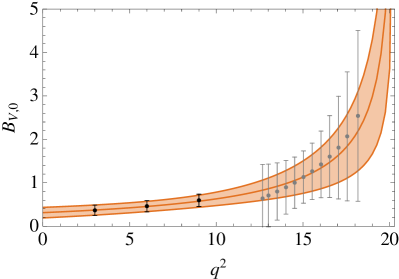
In our analysis, we will use the LCSR predictions from Refs. [8] and [9], taking 3(4) points at low values of q2superscript𝑞2q^{2} as input, see Table 3. The quoted errors are extrapolated from the value quoted for q2=0superscript𝑞20q^{2}=0 in the references specified in the Table. Lattice data is available for Bρ𝐵𝜌B\to\rho and BK𝐵𝐾B\to K decays, and is as shown in Table 4.555 We are very grateful to Sara Collins of the QCDSF collaboration for providing us with specific values for BK𝐵𝐾B\to K. For those data points which have an asymmetric statistical or systematic error, in order to perform the fit, we take the FF to be the central value in this statistical or systematic range, and take half the range to be the statistical or systematic error [34].

For Bρ𝐵𝜌B\to\rho and BK𝐵𝐾B\to K decays, we use LCSR and Lattice data to interpolate between the low and high–q2superscript𝑞2q^{2} region. The result can be compared to the case where we extrapolate to the high–q2superscript𝑞2q^{2} region only on the basis of LCSR predictions. This procedure will gives us an idea about the confidence in the extrapolations for those cases where Lattice data is lacking.

Table 3: Overview of LCSR points used, transformed to the helicity amplitude basis.
Decay FF LCSR/q2superscript𝑞2q^{2} (GeV2) Ref.
BK𝐵𝐾B\to K q2superscript𝑞2q^{2} 3 6 9 12 Table 3, [8]
𝒜V,0subscript𝒜𝑉0\mathcal{A}_{V,0} 0.40±0.05plus-or-minus0.400.050.40\pm 0.05 0.48±0.06plus-or-minus0.480.060.48\pm 0.06 0.59±0.07plus-or-minus0.590.070.59\pm 0.07 -
𝒜V,tsubscript𝒜𝑉𝑡\mathcal{A}_{V,t} 0.40±0.05plus-or-minus0.400.050.40\pm 0.05 0.51±0.06plus-or-minus0.510.060.51\pm 0.06 0.65±0.08plus-or-minus0.650.080.65\pm 0.08 -
𝒜T,0subscript𝒜𝑇0\mathcal{A}_{T,0} 0.13±0.01plus-or-minus0.130.010.13\pm 0.01 0.22±0.02plus-or-minus0.220.020.22\pm 0.02 0.34±0.03plus-or-minus0.340.030.34\pm 0.03 -
Bρ𝐵𝜌B\to\rho q2superscript𝑞2q^{2} 3 6 9 12 Table 8, [9]
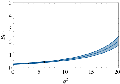
V,0subscript𝑉0\mathcal{B}_{V,0} 0.37±0.12plus-or-minus0.370.120.37\pm 0.12 0.46±0.13plus-or-minus0.460.130.46\pm 0.13 0.60±0.14plus-or-minus0.600.140.60\pm 0.14 -
V,1subscript𝑉1\mathcal{B}_{V,1} 0.16±0.01plus-or-minus0.160.010.16\pm 0.01 0.27±0.02plus-or-minus0.270.020.27\pm 0.02 0.41±0.04plus-or-minus0.410.040.41\pm 0.04 -
V,2subscript𝑉2\mathcal{B}_{V,2} 0.16±0.02plus-or-minus0.160.020.16\pm 0.02 0.29±0.03plus-or-minus0.290.030.29\pm 0.03 0.46±0.04plus-or-minus0.460.040.46\pm 0.04 -
V,tsubscript𝑉𝑡\mathcal{B}_{V,t} 0.37±0.04plus-or-minus0.370.040.37\pm 0.04 0.46±0.04plus-or-minus0.460.040.46\pm 0.04 0.58±0.06plus-or-minus0.580.060.58\pm 0.06 -
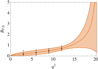
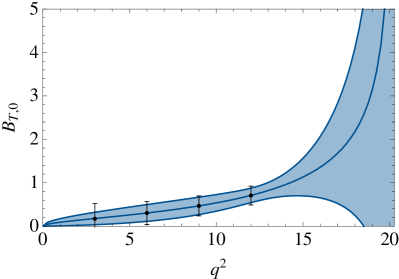
T,0subscript𝑇0\mathcal{B}_{T,0} 0.17±0.35plus-or-minus0.170.350.17\pm 0.35 0.3±0.26plus-or-minus0.30.260.3\pm 0.26 0.47±0.23plus-or-minus0.470.230.47\pm 0.23 0.71±0.22plus-or-minus0.710.220.71\pm 0.22
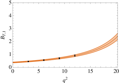
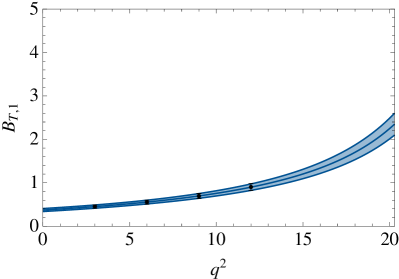
T,1subscript𝑇1\mathcal{B}_{T,1} 0.45±0.04plus-or-minus0.450.040.45\pm 0.04 0.55±0.05plus-or-minus0.550.050.55\pm 0.05 0.69±0.06plus-or-minus0.690.060.69\pm 0.06 0.9±0.08plus-or-minus0.90.080.9\pm 0.08
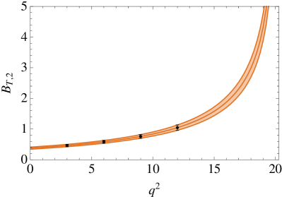
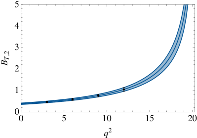
T,2subscript𝑇2\mathcal{B}_{T,2} 0.46±0.04plus-or-minus0.460.040.46\pm 0.04 0.58±0.05plus-or-minus0.580.050.58\pm 0.05 0.76±0.07plus-or-minus0.760.070.76\pm 0.07 1.0±0.1plus-or-minus1.00.11.0\pm 0.1
BK𝐵superscript𝐾B\to K^{*} q2superscript𝑞2q^{2} 3 6 9 12 Table 8, [9]
V,0subscript𝑉0\mathcal{B}_{V,0} 0.45±0.13plus-or-minus0.450.130.45\pm 0.13 0.56±0.13plus-or-minus0.560.130.56\pm 0.13 0.73±0.15plus-or-minus0.730.150.73\pm 0.15 -
V,1subscript𝑉1\mathcal{B}_{V,1} 0.19±0.02plus-or-minus0.190.020.19\pm 0.02 0.32±0.03plus-or-minus0.320.030.32\pm 0.03 0.49±0.04plus-or-minus0.490.040.49\pm 0.04 -
V,2subscript𝑉2\mathcal{B}_{V,2} 0.20±0.02plus-or-minus0.200.020.20\pm 0.02 0.35±0.03plus-or-minus0.350.030.35\pm 0.03 0.57±0.06plus-or-minus0.570.060.57\pm 0.06 -
V,tsubscript𝑉𝑡\mathcal{B}_{V,t} 0.44±0.04plus-or-minus0.440.040.44\pm 0.04 0.54±0.05plus-or-minus0.540.050.54\pm 0.05 0.67±0.06plus-or-minus0.670.060.67\pm 0.06 -
T,0subscript𝑇0\mathcal{B}_{T,0} 0.23±0.36plus-or-minus0.230.360.23\pm 0.36 0.39±0.27plus-or-minus0.390.270.39\pm 0.27 0.60±0.24plus-or-minus0.600.240.60\pm 0.24 0.90±0.22plus-or-minus0.900.220.90\pm 0.22
T,1subscript𝑇1\mathcal{B}_{T,1} 0.59±0.06plus-or-minus0.590.060.59\pm 0.06 0.72±0.07plus-or-minus0.720.070.72\pm 0.07 0.89±0.08plus-or-minus0.890.080.89\pm 0.08 1.2±0.1plus-or-minus1.20.11.2\pm 0.1
T,2subscript𝑇2\mathcal{B}_{T,2} 0.61±0.06plus-or-minus0.610.060.61\pm 0.06 0.77±0.07plus-or-minus0.770.070.77\pm 0.07 1.0±0.1plus-or-minus1.00.11.0\pm 0.1 1.4±0.1plus-or-minus1.40.11.4\pm 0.1
Bsϕsubscript𝐵𝑠italic-ϕB_{s}\to\phi q2superscript𝑞2q^{2} 3 6 9 12 Table 8, [9]
V,0subscript𝑉0\mathcal{B}_{V,0} 0.55±0.12plus-or-minus0.550.120.55\pm 0.12 0.68±0.13plus-or-minus0.680.130.68\pm 0.13 0.85±0.14plus-or-minus0.850.140.85\pm 0.14 -
V,1subscript𝑉1\mathcal{B}_{V,1} 0.2±0.02plus-or-minus0.20.020.2\pm 0.02 0.34±0.03plus-or-minus0.340.030.34\pm 0.03 0.52±0.04plus-or-minus0.520.040.52\pm 0.04 -
V,2subscript𝑉2\mathcal{B}_{V,2} 0.21±0.02plus-or-minus0.210.020.21\pm 0.02 0.38±0.04plus-or-minus0.380.040.38\pm 0.04 0.62±0.06plus-or-minus0.620.060.62\pm 0.06 -
V,tsubscript𝑉𝑡\mathcal{B}_{V,t} 0.56±0.04plus-or-minus0.560.040.56\pm 0.04 0.68±0.05plus-or-minus0.680.050.68\pm 0.05 0.85±0.06plus-or-minus0.850.060.85\pm 0.06 -
T,0subscript𝑇0\mathcal{B}_{T,0} 0.26±0.39plus-or-minus0.260.390.26\pm 0.39 0.44±0.29plus-or-minus0.440.290.44\pm 0.29 0.67±0.26plus-or-minus0.670.260.67\pm 0.26 1.0±0.3plus-or-minus1.00.31.0\pm 0.3
T,1subscript𝑇1\mathcal{B}_{T,1} 0.59±0.06plus-or-minus0.590.060.59\pm 0.06 0.72±0.07plus-or-minus0.720.070.72\pm 0.07 0.89±0.08plus-or-minus0.890.080.89\pm 0.08 1.2±0.1plus-or-minus1.20.11.2\pm 0.1
T,2subscript𝑇2\mathcal{B}_{T,2} 0.61±0.06plus-or-minus0.610.060.61\pm 0.06 0.77±0.07plus-or-minus0.770.070.77\pm 0.07 1.0±0.1plus-or-minus1.00.11.0\pm 0.1 1.4±0.1plus-or-minus1.40.11.4\pm 0.1
Table 4: Overview of Lattice points used, transformed to the helicity amplitude basis. Note that specific values for Bρ𝐵𝜌B\to\rho are as in Table 2 of Ref. [12].
Decay q2superscript𝑞2q^{2} (GeV2) FF Ref.
BK𝐵𝐾B\to K 𝒜V,0subscript𝒜𝑉0\mathcal{A}_{V,0} 𝒜V,tsubscript𝒜𝑉𝑡\mathcal{A}_{V,t} 𝒜T,0subscript𝒜𝑇0\mathcal{A}_{T,0} QCDSF [4]
14.5 0.94±0.19plus-or-minus0.940.190.94\pm 0.19 1.1±0.2plus-or-minus1.10.21.1\pm 0.2 -
15.6 1.1±0.2plus-or-minus1.10.21.1\pm 0.2 1.3±0.3plus-or-minus1.30.31.3\pm 0.3 -
16.7 1.2±0.2plus-or-minus1.20.21.2\pm 0.2 1.5±0.3plus-or-minus1.50.31.5\pm 0.3 -
17.9 1.4±0.3plus-or-minus1.40.31.4\pm 0.3 1.8±0.3plus-or-minus1.80.31.8\pm 0.3 -
19. 1.6±0.3plus-or-minus1.60.31.6\pm 0.3 2.3±0.4plus-or-minus2.30.42.3\pm 0.4 -
20.1 1.9±0.4plus-or-minus1.90.41.9\pm 0.4 3.±0.6formulae-sequence3plus-or-minus0.63.\pm 0.6 -
21.3 2.3±0.4plus-or-minus2.30.42.3\pm 0.4 4.4±0.8plus-or-minus4.40.84.4\pm 0.8 -
22.4 2.9±0.6plus-or-minus2.90.62.9\pm 0.6 8.7±1.7plus-or-minus8.71.78.7\pm 1.7 -
Bρ𝐵𝜌B\to\rho V,0subscript𝑉0\mathcal{B}_{V,0} V,1subscript𝑉1\mathcal{B}_{V,1} T,2subscript𝑇2\mathcal{B}_{T,2} UKQCD [7]
12.7 0.64±0.78plus-or-minus0.640.780.64\pm 0.78 0.34±0.27plus-or-minus0.340.270.34\pm 0.27 0.9±0.18plus-or-minus0.90.180.9\pm 0.18
13. 0.71±0.72plus-or-minus0.710.720.71\pm 0.72 0.39±0.25plus-or-minus0.390.250.39\pm 0.25 0.96±0.18plus-or-minus0.960.180.96\pm 0.18
13.5 0.8±0.66plus-or-minus0.80.660.8\pm 0.66 0.48±0.22plus-or-minus0.480.220.48\pm 0.22 1.1±0.2plus-or-minus1.10.21.1\pm 0.2
14. 0.9±0.62plus-or-minus0.90.620.9\pm 0.62 0.58±0.19plus-or-minus0.580.190.58\pm 0.19 1.2±0.2plus-or-minus1.20.21.2\pm 0.2
14.5 1.0±0.6plus-or-minus1.00.61.0\pm 0.6 0.68±0.16plus-or-minus0.680.160.68\pm 0.16 1.3±0.2plus-or-minus1.30.21.3\pm 0.2
15. 1.1±0.6plus-or-minus1.10.61.1\pm 0.6 0.78±0.15plus-or-minus0.780.150.78\pm 0.15 1.4±0.2plus-or-minus1.40.21.4\pm 0.2
15.5 1.3±0.7plus-or-minus1.30.71.3\pm 0.7 0.89±0.15plus-or-minus0.890.150.89\pm 0.15 1.6±0.2plus-or-minus1.60.21.6\pm 0.2
16. 1.4±0.8plus-or-minus1.40.81.4\pm 0.8 1.0±0.2plus-or-minus1.00.21.0\pm 0.2 1.8±0.2plus-or-minus1.80.21.8\pm 0.2
16.5 1.6±0.9plus-or-minus1.60.91.6\pm 0.9 1.2±0.3plus-or-minus1.20.31.2\pm 0.3 2.1±0.2plus-or-minus2.10.22.1\pm 0.2
17.1 1.8±1.2plus-or-minus1.81.21.8\pm 1.2 1.4±0.4plus-or-minus1.40.41.4\pm 0.4 2.4±0.2plus-or-minus2.40.22.4\pm 0.2
17.6 2.1±1.5plus-or-minus2.11.52.1\pm 1.5 1.7±0.6plus-or-minus1.70.61.7\pm 0.6 2.7±0.3plus-or-minus2.70.32.7\pm 0.3
18.2 2.5±2.plus-or-minus2.522.5\pm 2. 2.1±0.9plus-or-minus2.10.92.1\pm 0.9 3.3±0.3plus-or-minus3.30.33.3\pm 0.3

4.2 Parameterisation of FFs as Series Expansion

For those channels where where Lattice data is not available, it is essential to employ a FF parameterisation that takes into account the characteristic features of the FF shape as determined from the analyticity and unitarity consideration above. For every considered FF, we will therefore define a parameterisation based on the SE,

𝒜V,0(t)subscript𝒜𝑉0𝑡\displaystyle{\cal A}_{V,0}(t) =1B(t)ϕTV(t)k=0K1αk(V,0)zk,absent1𝐵𝑡superscriptsubscriptitalic-ϕ𝑇𝑉𝑡superscriptsubscript𝑘0𝐾1subscriptsuperscript𝛼𝑉0𝑘superscript𝑧𝑘\displaystyle=\frac{1}{B(t)\,\phi_{T}^{V}(t)}\,\sum_{k=0}^{K-1}\alpha^{(V,0)}_{k}\,z^{k}\,, (51)
𝒜V,t(t)subscript𝒜𝑉𝑡𝑡\displaystyle{\cal A}_{V,t}(t) =1B(t)z(t,t)ϕLV(t)k=0K1αk(V,t)zk,absent1𝐵𝑡𝑧𝑡subscript𝑡superscriptsubscriptitalic-ϕ𝐿𝑉𝑡superscriptsubscript𝑘0𝐾1subscriptsuperscript𝛼𝑉𝑡𝑘superscript𝑧𝑘\displaystyle=\frac{1}{B(t)\,\sqrt{z(t,t_{-})}\,\phi_{L}^{V}(t)}\,\sum_{k=0}^{K-1}\alpha^{(V,t)}_{k}\,z^{k}\,, (52)
𝒜T,0(t)subscript𝒜𝑇0𝑡\displaystyle{\cal A}_{T,0}(t) =z(t,0)B(t)ϕTT(t)k=0K1αk(T,0)zk,absent𝑧𝑡0𝐵𝑡superscriptsubscriptitalic-ϕ𝑇𝑇𝑡superscriptsubscript𝑘0𝐾1subscriptsuperscript𝛼𝑇0𝑘superscript𝑧𝑘\displaystyle=\frac{\sqrt{-z(t,0)}}{B(t)\,\phi_{T}^{T}(t)}\,\sum_{k=0}^{K-1}\alpha^{(T,0)}_{k}\,z^{k}\,, (53)

and

V,t(t)subscript𝑉𝑡𝑡\displaystyle{\cal B}_{V,t}(t) =1B(t)ϕLVA(t)k=0K1βk(V,t)zk,absent1𝐵𝑡superscriptsubscriptitalic-ϕ𝐿𝑉𝐴𝑡superscriptsubscript𝑘0𝐾1subscriptsuperscript𝛽𝑉𝑡𝑘superscript𝑧𝑘\displaystyle=\frac{1}{B(t)\,\phi_{L}^{V-A}(t)}\,\sum_{k=0}^{K-1}\beta^{(V,t)}_{k}\,z^{k}\,, (54)
T,0(t)subscript𝑇0𝑡\displaystyle{\cal B}_{T,0}(t) =z(t,0)B(t)z(t,t)ϕTT+AT(t)k=0K1βk(T,0)zk,absent𝑧𝑡0𝐵𝑡𝑧𝑡subscript𝑡superscriptsubscriptitalic-ϕ𝑇𝑇subscript𝐴𝑇𝑡superscriptsubscript𝑘0𝐾1subscriptsuperscript𝛽𝑇0𝑘superscript𝑧𝑘\displaystyle=\frac{\sqrt{-z(t,0)}}{B(t)\,\sqrt{z(t,t_{-})}\,\phi_{T}^{T+A_{T}}(t)}\,\sum_{k=0}^{K-1}\beta^{(T,0)}_{k}\,z^{k}\,, (55)
T,1(t)subscript𝑇1𝑡\displaystyle{\cal B}_{T,1}(t) =1B(t)ϕTT+AT(t)k=0K1βk(T,1)zk,absent1𝐵𝑡superscriptsubscriptitalic-ϕ𝑇𝑇subscript𝐴𝑇𝑡superscriptsubscript𝑘0𝐾1subscriptsuperscript𝛽𝑇1𝑘superscript𝑧𝑘\displaystyle=\frac{1}{B(t)\,\phi_{T}^{T+A_{T}}(t)}\,\sum_{k=0}^{K-1}\beta^{(T,1)}_{k}\,z^{k}\,, (56)
T,2(t)subscript𝑇2𝑡\displaystyle{\cal B}_{T,2}(t) =1B(t)z(t,t)ϕTT+AT(t)k=0K1βk(T,2)zk,absent1𝐵𝑡𝑧𝑡subscript𝑡superscriptsubscriptitalic-ϕ𝑇𝑇subscript𝐴𝑇𝑡superscriptsubscript𝑘0𝐾1subscriptsuperscript𝛽𝑇2𝑘superscript𝑧𝑘\displaystyle=\frac{1}{B(t)\,\sqrt{z(t,t_{-})}\,\phi_{T}^{T+A_{T}}(t)}\,\sum_{k=0}^{K-1}\beta^{(T,2)}_{k}\,z^{k}\,, (57)

and V,02subscript𝑉02{\cal B}_{V,0-2} already given in (49). Here we have used our FF convention defined in (5,8,10,15) and explicitly quoted the pre-factors, necessary to obtain the correct analytical behaviour of our FFs.666In Refs. [18] and [17, 13], the predictions from perturbative QCD for the scaling of the FFs at large values of q2superscript𝑞2q^{2} have been used as an additional constraint on the shape of the FFs. We have found that these constraints do not influence the FF fits in the decay region significantly. As the asymptotic behaviour of exclusive observables in QCD is still a matter of controversy, we therefore find it safer and simpler not to include these constraints in our parameterisation. In our fits below, we will find that in general the SE can be truncated after the first two terms, i.e. the parameter K𝐾K can be set to 2. We should point out, however, that this does not necessarily imply that higher-order terms in the SE are negligible: Although |z|21much-less-thansuperscript𝑧21|z|^{2}\ll 1 in the semi-leptonic region, one may still have |α2z2||α1z|similar-tosubscript𝛼2superscript𝑧2subscript𝛼1𝑧|\alpha_{2}\,z^{2}|\sim|\alpha_{1}z| if the coefficients satisfy α1α21much-less-thansubscript𝛼1subscript𝛼2less-than-or-similar-to1\alpha_{1}\ll\alpha_{2}\lesssim 1. From the theoretical point of view, this reflects an irreducible source of uncertainty, which we will discuss in some detail for some specific examples in Sec. 4.4. From the practical point of view, we consider the truncated SE as a reasonable parameterisation which is easy to implement (and easy to refine) in phenomenological studies.

For simplicity, we will not explicitly implement the theoretical relations (80,82), that some of the FFs fulfil at q2=0superscript𝑞20q^{2}=0, into the fit, because they are automatically satisfied by the rather precise input from LCSR at this point. However, the helicity-based FF definition further implies a relation between the FFs V,0subscript𝑉0{\cal B}_{V,0} and V,2subscript𝑉2{\cal B}_{V,2}, and similarly between T,0subscript𝑇0{\cal B}_{T,0} and T,2subscript𝑇2{\cal B}_{T,2}, see (83) in the appendix, which we will implement as an additional constraints on the corresponding coefficients in the SE. From the above parameterisations, the SSE is obtained by the replacements

ϕIX(t)superscriptsubscriptitalic-ϕ𝐼𝑋𝑡\displaystyle\phi_{I}^{X}(t) 1,B(t)P(t),z(t,0)q2/mB,z(t,t)λ/mB2,formulae-sequenceabsent1formulae-sequence𝐵𝑡𝑃𝑡formulae-sequence𝑧𝑡0superscript𝑞2subscript𝑚𝐵𝑧𝑡subscript𝑡𝜆superscriptsubscript𝑚𝐵2\displaystyle\to 1\,,\quad B(t)\to P(t)\,,\quad\sqrt{-z(t,0)}\to\sqrt{q^{2}}/m_{B}\,,\quad\sqrt{z(t,t_{-})}\to\sqrt{\lambda}/m_{B}^{2}\,, (58)

with new coefficients α~ksubscript~𝛼𝑘\tilde{\alpha}_{k} and β~ksubscript~𝛽𝑘\tilde{\beta}_{k}.

4.2.1 Unitarity constraints

For the SE parameterisation, the unitarity constraints take the form

k=0K1(αk)21for 𝒜V,0 and 𝒜T,0,3k=0K1(αk)21for 𝒜V,t,formulae-sequencesuperscriptsubscript𝑘0𝐾1superscriptsubscript𝛼𝑘21for 𝒜V,0 and 𝒜T,0,3superscriptsubscript𝑘0𝐾1superscriptsubscript𝛼𝑘21for 𝒜V,t,\displaystyle\sum_{k=0}^{K-1}\,(\alpha_{k})^{2}\leq 1\quad\mbox{for ${\cal A}_{V,0}$ and ${\cal A}_{T,0}$,}\qquad 3\sum_{k=0}^{K-1}\,(\alpha_{k})^{2}\leq 1\quad\mbox{for ${\cal A}_{V,t}$,} (59)

and

33\displaystyle 3 k=0K1(βk(V,t))21for V,t,superscriptsubscript𝑘0𝐾1superscriptsuperscriptsubscript𝛽𝑘𝑉𝑡21for V,t,\displaystyle\sum_{k=0}^{K-1}\,(\beta_{k}^{(V,t)})^{2}\leq 1\quad\mbox{for ${\cal B}_{V,t}$,} (60)
k=0K1{(βk(V,0))2+(βk(V,1))2+(βk(V,2))2}1for V,0V,1, and V,2,superscriptsubscript𝑘0𝐾1superscriptsuperscriptsubscript𝛽𝑘𝑉02superscriptsuperscriptsubscript𝛽𝑘𝑉12superscriptsuperscriptsubscript𝛽𝑘𝑉221for V,0V,1, and V,2,\displaystyle\sum_{k=0}^{K-1}\left\{(\beta_{k}^{(V,0)})^{2}+(\beta_{k}^{(V,1)})^{2}+(\beta_{k}^{(V,2)})^{2}\right\}\leq 1\quad\mbox{for ${\cal B}_{V,0}$, ${\cal B}_{V,1}$, and ${\cal B}_{V,2}$,} (61)
k=0K1{(βk(T,0))2+(βk(T,1))2+(βk(T,2))2}1for T,0T,1, and T,2.superscriptsubscript𝑘0𝐾1superscriptsuperscriptsubscript𝛽𝑘𝑇02superscriptsuperscriptsubscript𝛽𝑘𝑇12superscriptsuperscriptsubscript𝛽𝑘𝑇221for T,0T,1, and T,2.\displaystyle\sum_{k=0}^{K-1}\left\{(\beta_{k}^{(T,0)})^{2}+(\beta_{k}^{(T,1)})^{2}+(\beta_{k}^{(T,2)})^{2}\right\}\leq 1\quad\mbox{for ${\cal B}_{T,0}$, ${\cal B}_{T,1}$, and ${\cal B}_{T,2}$.} (62)

For the SSE parameterisation, imposing the unitarity bound is more complicated, as shown in Ref. [13]. We repeat the derivation of this bound in order to define notation used later. One first compares the SE and SSE parameterisations:

k=0K1αkzk=Λ(z)k=0K1α~kzksuperscriptsubscript𝑘0𝐾1subscript𝛼𝑘superscript𝑧𝑘Λ𝑧superscriptsubscript𝑘0𝐾1subscript~𝛼𝑘superscript𝑧𝑘\sum_{k=0}^{K-1}\,\alpha_{k}\,z^{k}=\Lambda(z)\sum_{k=0}^{K-1}\tilde{\alpha}_{k}\,z^{k} (63)

One can simply obtain Λ(z)Λ𝑧\Lambda(z) by combining the prefactors from the SE expansion with the prefactors from the SSE expansion, and expressing the result as a function of z(t,t0)𝑧𝑡subscript𝑡0z(t,t_{0}). Since z𝑧z is a small parameter, we can expand Λ(z)Λ𝑧\Lambda(z) in powers of z𝑧z:

Λ(z)=kζkzk.Λ𝑧subscript𝑘subscript𝜁𝑘superscript𝑧𝑘\Lambda(z)=\sum_{k}\,\zeta_{k}\,z^{k}. (64)

We can therefore obtain a relation between the coefficients αksubscript𝛼𝑘\alpha_{k} and α~ksubscript~𝛼𝑘\tilde{\alpha}_{k},

αi=k=0min[K1,i]ζikα~k,0iK1,formulae-sequencesubscript𝛼𝑖superscriptsubscript𝑘0min𝐾1𝑖subscript𝜁𝑖𝑘subscript~𝛼𝑘0𝑖𝐾1\alpha_{i}=\sum_{k=0}^{\mathrm{min}[K-1,i]}\zeta_{i-k}\,\tilde{\alpha}_{k}\,,\qquad 0\leq i\leq K-1\,, (65)

which results in bounds of the type

j,k=0K1Cjkα~jα~k1,superscriptsubscript𝑗𝑘0𝐾1subscript𝐶𝑗𝑘subscript~𝛼𝑗subscript~𝛼𝑘1\sum_{j,k=0}^{K-1}C_{jk}\,\tilde{\alpha}_{j}\,\tilde{\alpha}_{k}\leq 1\,, (66)

where

Cjk=i=0K1max[j,k]ζiζi+|jk|subscript𝐶𝑗𝑘superscriptsubscript𝑖0𝐾1max𝑗𝑘subscript𝜁𝑖subscript𝜁𝑖𝑗𝑘C_{jk}=\sum_{i=0}^{K-1-\mathrm{max}[j,k]}\zeta_{i}\,\zeta_{i+|j-k|} (67)

is a positive definite matrix.

4.3 Fitting prescription

We perform a fit to the LCSR data, as well as, where possible, a combined fit to the LCSR and Lattice data, by minimising a χ2superscript𝜒2\chi^{2} function defined by

χ2(θ)=(FiF(ti,θ))[V1]ij(FjF(tj,θ)),superscript𝜒2𝜃subscript𝐹𝑖𝐹subscript𝑡𝑖𝜃subscriptdelimited-[]superscript𝑉1𝑖𝑗subscript𝐹𝑗𝐹subscript𝑡𝑗𝜃\chi^{2}(\vec{\theta})=\left(F_{i}-F(t_{i},\vec{\theta}\,)\right)\left[V^{-1}\right]_{ij}\!\left(F_{j}-F(t_{j},\vec{\theta}\,)\right)\,, (68)

where θ𝜃\vec{\theta} contains the parameters of a given FF parameterisation, Fisubscript𝐹𝑖F_{i} are the FF values from LCSR/Lattice at given points tisubscript𝑡𝑖t_{i}, and Vijsubscript𝑉𝑖𝑗V_{ij} are elements of the covariance matrix as defined below.

As explained above, we are going to investigate parameterisations based on two variants of the SE, where the parameters will be subject to additional constraints derived from dispersive bounds on the FFs.

  • In the conventional series expansion (SE), we use (19), and truncate the series after the first 2 terms, such that

    θ={α0,α1},αi2<!1.formulae-sequence𝜃subscript𝛼0subscript𝛼1superscriptsuperscriptsubscript𝛼𝑖21\vec{\theta}=\{\alpha_{0},\alpha_{1}\}\,,\qquad\sum\alpha_{i}^{2}\stackrel{{\scriptstyle!}}{{<}}1\,.
  • The simplified series expansion (SSE) uses (22), with

    θ={α~0,α~1},i,j=01Cijα~iα~j<!1,formulae-sequence𝜃subscript~𝛼0subscript~𝛼1superscriptsuperscriptsubscript𝑖𝑗01subscript𝐶𝑖𝑗subscript~𝛼𝑖subscript~𝛼𝑗1\vec{\theta}=\{\tilde{\alpha}_{0},\tilde{\alpha}_{1}\}\,,\qquad\sum_{i,j=0}^{1}C_{ij}\,\tilde{\alpha}_{i}\tilde{\alpha}_{j}\stackrel{{\scriptstyle!}}{{<}}1\,,

    where the matrix Cijsubscript𝐶𝑖𝑗C_{ij} is defined in (67).

In constructing the covariance matrix, when we do a combined fit to LCSR and Lattice data, we assume the matrix to be block diagonal with independent blocks for Lattice and LCSR, equivalent to χ2=χLCSR2+χLat2superscript𝜒2superscriptsubscript𝜒LCSR2superscriptsubscript𝜒Lat2\chi^{2}=\chi_{\rm LCSR}^{2}+\chi_{\rm Lat}^{2}, where

χLCSR2(θ)=(FiF(ti,θ))[VLCSR1]ij(FjF(tj,θ)),superscriptsubscript𝜒LCSR2𝜃subscript𝐹𝑖𝐹subscript𝑡𝑖𝜃subscriptdelimited-[]superscriptsubscript𝑉LCSR1𝑖𝑗subscript𝐹𝑗𝐹subscript𝑡𝑗𝜃\chi_{\rm LCSR}^{2}(\vec{\theta})=\left(F_{i}-F(t_{i},\vec{\theta}\,)\right)\left[V_{\rm LCSR}^{-1}\right]_{ij}\!\left(F_{j}-F(t_{j},\vec{\theta}\,)\right)\,, (69)

and

χLat2(θ)=(FiF(ti,θ))[VLat1]ij(FjF(tj,θ)),superscriptsubscript𝜒Lat2𝜃subscript𝐹𝑖𝐹subscript𝑡𝑖𝜃subscriptdelimited-[]superscriptsubscript𝑉Lat1𝑖𝑗subscript𝐹𝑗𝐹subscript𝑡𝑗𝜃\chi_{\rm Lat}^{2}(\vec{\theta})=\left(F_{i}-F(t_{i},\vec{\theta}\,)\right)\left[V_{\rm Lat}^{-1}\right]_{ij}\!\left(F_{j}-F(t_{j},\vec{\theta}\,)\right)\,, (70)

We consider the statistical and systematic contributions to the Lattice errors separately. Where results were not available in the literature, we received the breakdown by private communication with the authors. In obtaining the covariance matrix, we make the following conservative assumptions:

  • Statistical errors of Lattice data are 50%percent5050\% correlated [4, 7].

  • Systematic errors of Lattice data are 100%percent100100\% correlated [4, 7].

  • Errors of LCSR data are due to parametric as well as to systematic uncertainties from different sources. In order to provide a concrete number for the χ2superscript𝜒2\chi^{2} value characeterizing the quality of the fit, we have estimated the errors of LCSR data at different values tisubscript𝑡𝑖t_{i} to be 75%percent7575\% correlated.777We have checked that using 90%percent9090\% or 50%percent5050\% correlation, instead — of course — globally changes the very value of χ2superscript𝜒2\chi^{2}, but does not influence the optimal parameter values. A similar comment applies to the number of individual LCSR points used in the fit.

This prescription leads to a covariance matrix Vij=cov[ti,tj]superscript𝑉𝑖𝑗covsuperscripttisuperscripttjV^{ij}=\rm{cov}[t^{i},t^{j}], containing

VLCSRijsuperscriptsubscript𝑉LCSR𝑖𝑗\displaystyle V_{\rm LCSR}^{ij} =\displaystyle= 14κiκjδij+34κiκjand14superscript𝜅𝑖superscript𝜅𝑗subscript𝛿𝑖𝑗34superscript𝜅𝑖superscript𝜅𝑗and\displaystyle\frac{1}{4}\kappa^{i}\kappa^{j}\delta_{ij}+\frac{3}{4}\kappa^{i}\kappa^{j}\qquad\mathrm{and} (71)
VLatijsuperscriptsubscript𝑉Lat𝑖𝑗\displaystyle V_{\rm Lat}^{ij} =\displaystyle= 12σiσjδij+12σiσj+εiεj12superscript𝜎𝑖superscript𝜎𝑗subscript𝛿𝑖𝑗12superscript𝜎𝑖superscript𝜎𝑗superscript𝜀𝑖superscript𝜀𝑗\displaystyle\frac{1}{2}\sigma^{i}\sigma^{j}\delta_{ij}+\frac{1}{2}\sigma^{i}\sigma^{j}+\varepsilon^{i}\varepsilon^{j} (72)

where σisubscript𝜎𝑖\sigma_{i} are the statistical errors, εisubscript𝜀𝑖\varepsilon_{i} are the systematic errors for the Lattice data, and κisubscript𝜅𝑖\kappa_{i} are the errors for the LCSR predictions.

Minimising χ2(θ)superscript𝜒2𝜃\chi^{2}(\vec{\theta}) then yields the best fit parameters θsuperscript𝜃\vec{\theta}^{*}, as well as the covariance matrix of the fit, Uij=cov[θi,θj]subscript𝑈𝑖𝑗covsubscript𝜃isubscript𝜃jU_{ij}=\rm{cov}[\theta_{i},\theta_{j}],

(U1)ij=122χ2(θ)θiθj|θ=θ,subscriptsuperscript𝑈1𝑖𝑗evaluated-at12superscript2superscript𝜒2𝜃subscript𝜃𝑖subscript𝜃𝑗𝜃superscript𝜃\left({U^{-1}}\right)_{ij}=\frac{1}{2}\left.{\frac{{\partial^{2}\chi^{2}(\vec{\theta})}}{{\partial\theta_{i}\,\partial\theta_{j}}}}\right|_{\vec{\theta}=\vec{\theta}^{*}}\,, (73)

from which we calculate the error associated to the fitted FF function:

ΔF(t,θ)=F(t,θ)θi|θ=θUijF(t,θ)θj|θ=θΔ𝐹𝑡superscript𝜃evaluated-atevaluated-at𝐹𝑡𝜃subscript𝜃𝑖𝜃superscript𝜃subscript𝑈𝑖𝑗𝐹𝑡𝜃subscript𝜃𝑗𝜃superscript𝜃\Delta F(t,\vec{\theta}^{*})={\left.{\frac{{\partial F(t,\vec{\theta})}}{{\partial\theta_{i}}}}\right|_{\vec{\theta}=\vec{\theta}^{*}}}\,U_{ij}\,{\left.{\frac{{\partial F(t,\vec{\theta})}}{{\partial\theta_{j}}}}\right|_{\vec{\theta}=\vec{\theta}^{*}}} (74)

4.4 Results

Having established the fitting procedure, we consider FFs for the decays Bρ𝐵𝜌B\to\rho, BK𝐵𝐾B\to K, BK𝐵superscript𝐾B\to K^{*} and Bsϕsubscript𝐵𝑠italic-ϕB_{s}\to\phi. We concentrate on radiative and rare semi-leptonic decays, as previously the dispersive bounds had not been calculated for the tensor current, so could not be applied to these decays. The phenomenological motivations for studying the chosen decays are as follows. First, they involve flavour changing neutral currents via e.g. electroweak penguins, so they are particularly sensitive to new physics. Secondly, the di-lepton signature can easily be detected at the LHC, and the three-body or four-body final state (for subsequent decays KKπsuperscript𝐾𝐾𝜋K^{*}\to K\pi and ϕKKitalic-ϕ𝐾𝐾\phi\to KK) involves many promising observables related to various angular distributions [22, 35, 20, 36, 21].

From the theoretical point of view, the BVγ𝐵𝑉𝛾B\to V\gamma decay as well as the low-q2superscript𝑞2q^{2} region of BL+𝐵𝐿superscriptsuperscriptB\to L\,\ell^{+}\ell^{-} transitions allow for a systematic inclusion of radiative corrections within the QCD factorization approach at leading order in the 1/mb1subscript𝑚𝑏1/m_{b} expansion [37, 19]. In this region, the transition FFs (which still determine a major part of non-perturbative input) can be obtained from LCSR estimates alone. As it has been discussed, for instance, in [38], the high-q2superscript𝑞2q^{2} region may also be interesting in order to constrain NP contributions (notably to the short-distance Wilson coefficients C9subscript𝐶9C_{9} and C10subscript𝐶10C_{10}), and therefore our extrapolations of LCSR results for the tensor FFs in that region will be particularly relevant for this purpose. In the following subsection, we present the results of fitting the specific FFs to both, the SE and SSE parameterisations, using LCSR and Lattice data where appropriate as discussed in Section 4.1. For the light meson masses, we use mK=494subscript𝑚𝐾494m_{K}=494 MeV, mK=892subscript𝑚superscript𝐾892m_{K^{*}}=892 MeV, mρ=776subscript𝑚𝜌776m_{\rho}=776 MeV, mϕ=1.02subscript𝑚italic-ϕ1.02m_{\phi}=1.02 GeV.

𝑩𝑲bold-→𝑩𝑲B\to K form factors:

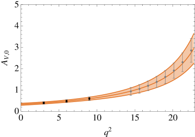
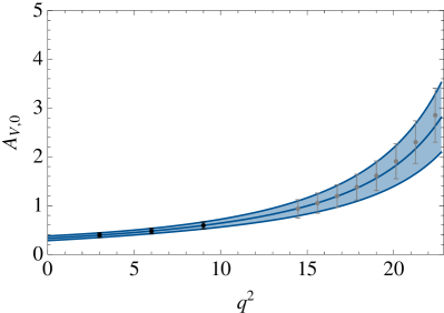
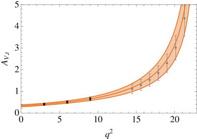
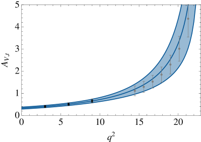
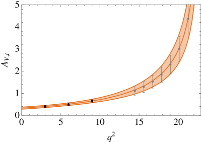
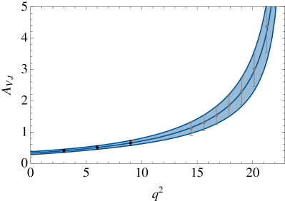
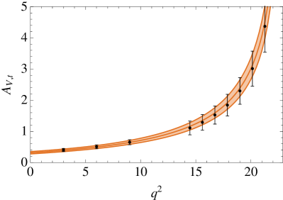
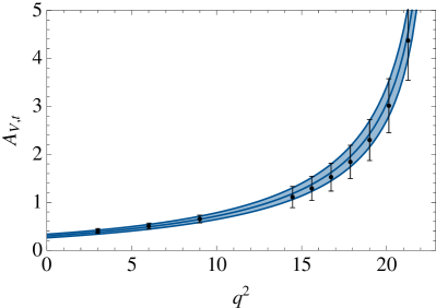
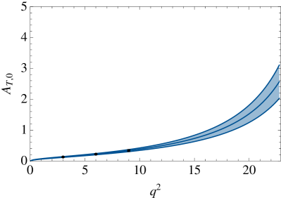
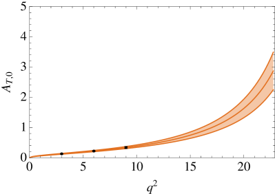
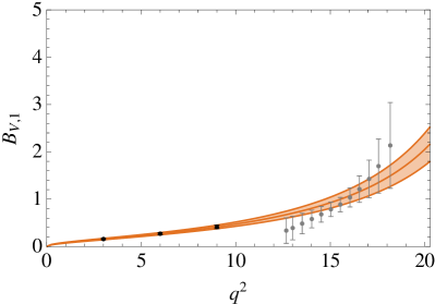
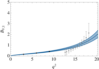
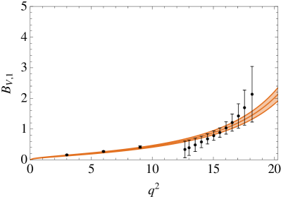
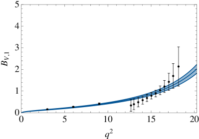
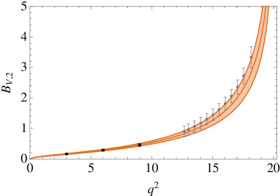
In Figs. 15, we show the fit for the various BK𝐵𝐾B\to K FFs, which enter, for instance, the radiative BK+𝐵𝐾superscriptsuperscriptB\to K\ell^{+}\ell^{-} and BKνν¯𝐵𝐾𝜈¯𝜈B\to K\nu\bar{\nu} decays. We compare the result of the SE and SSE parameterisations using LCSR data, and investigate the changes when the Lattice data is included. The numerical results for the best-fit parameters of the SE and SSE fit are found in corresponding Tables 56. The covariance matrices for these fits can also be found in Appendix E.

Generally, both parameterisations are seen to fit the data well, and importantly, we find agreement with the Lattice predictions for 𝒜V,0subscript𝒜𝑉0\mathcal{A}_{V,0} and 𝒜V,tsubscript𝒜𝑉𝑡\mathcal{A}_{V,t}, even when they are not included in the fit. We therefore consider our extrapolation of LCSR data for the tensor FF 𝒜T,0subscript𝒜𝑇0\mathcal{A}_{T,0} to the high-q2superscript𝑞2q^{2} region, where Lattice data does not exist, as sufficiently reliable. The quality of the fits is astonishingly good, considering the χ2superscript𝜒2\chi^{2} values for only two free parameters in the expansion. The differences between the SE and SSE are only marginal, which can be traced back to the usage of the optimised value for the auxiliary parameter t0subscript𝑡0t_{0} in (21). The dispersive bounds turn out to be far from being separated, and therefore they have only little impact on the FF fit. This observation is in line with other studies of heavy-to-light FFs in the literature, see e.g. [18, 14, 39].

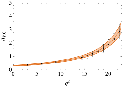
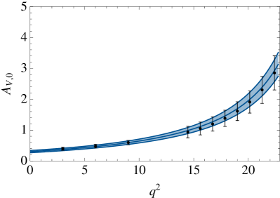
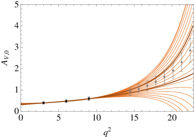
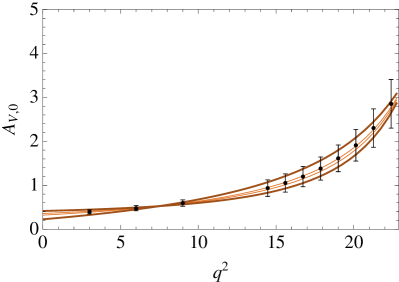
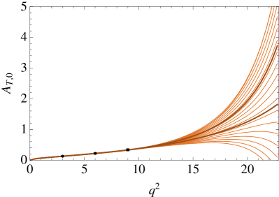
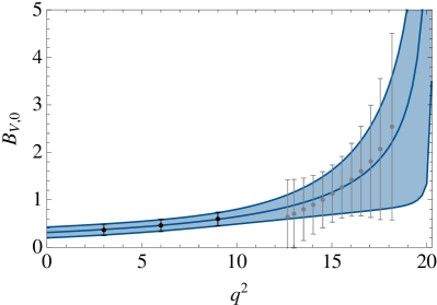
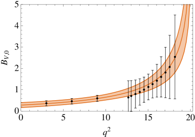
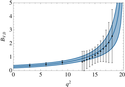
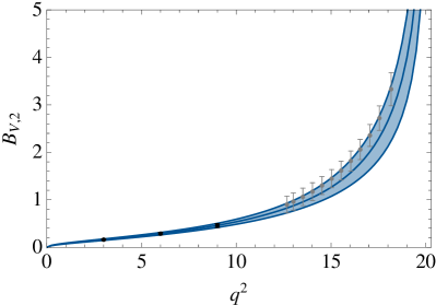
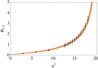
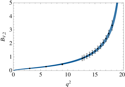
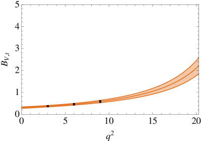
In order to address the question of potential contributions from higher-order terms in the SE, we consider the LCSR prediction for the vector and tensor form factors 𝒜V,0subscript𝒜𝑉0{\cal A}_{V,0}, 𝒜T,0subscript𝒜𝑇0{\cal A}_{T,0} and fit to a SE with K=3𝐾3K=3, where the coefficient a2subscript𝑎2a_{2} of the z2superscript𝑧2z^{2} term in the expansion has been fixed to values between [0.9,+0.9]0.90.9[-0.9,+0.9], representing almost the maximal range allowed by the unitarity constraints. The results of these fits are shown in Figs. 2,6. Let us first consider the case, where only LCSR data is used in the fit. We observe that — as expected — the constraints from the LCSR points at low values of q2superscript𝑞2q^{2} are not sufficient to determine the behaviour at large q2superscript𝑞2q^{2}, if higher-order terms in the SE (with no further phenomenological constraints) are allowed for. However, the behaviour of the form factor corresponding to the extreme values of a2subscript𝑎2a_{2} does not appear very realistic (even a rough numerical estimate of coupling constants for the first low-lying resonances with the considered hadronic transition would be sufficient to exclude the curves at the margin). Therefore the associated error estimate appears too pessimistic to us. Moreover, typically, exclusive semi-leptonic branching fractions are suppressed relative to the inclusive ones by a factor of about 20. This suggests that the right-hand side of the dispersive bounds should not exceed a value of 5% (instead of 100%). Correspondingly, a realistic range of allowed a2subscript𝑎2a_{2}–values should rather be taken as [0.25,+0.25]0.250.25[-0.25,+0.25], which is indicated by the thick central lines in Fig. 2. The associated uncertainty is only slightly larger than the one obtained from the variation of (a0,a1)subscript𝑎0subscript𝑎1(a_{0},a_{1}) for the SE fit with K=2𝐾2K=2. If, on the other hand, the lattice information (in the case of 𝒜V,0subscript𝒜𝑉0{\cal A}_{V,0}) is taken into account, the cases with |a2|0.25greater-than-or-equivalent-tosubscript𝑎20.25|a_{2}|\gtrsim 0.25 actually do not yield a satisfactoring fit anymore, and again the error estimate of the linear fit seems to be sufficient to estimate the fit errors. In view of the generic difficulties in estimating systematic theoretical uncertainties, we thus consider the SE/SSE parameterisation with K=2𝐾2K=2 and the associated error estimates as sufficiently reliable for practical applications.

Another comment applies to the scalar FFs 𝒜V,tsubscript𝒜𝑉𝑡{\cal A}_{V,t}: As shown in Table 1, the combined heavy-quark/chiral-symmetry limit considered in [26] predicts a scalar Bssubscript𝐵𝑠B_{s} resonance below BK𝐵𝐾BK-production threshold (such a state is also favoured by a Lattice computation in [40]). On the other hand, the PDG only finds resonances at masses near/above the production threshold. We have therefore chosen to compare two variants of the fit, with/without a scalar resonance.888Notice that BZ [8] use an effective resonance mass above production threshold to parameterise the scalar FFs. As can be seen, the fit with a scalar resonance from [26] describes the combined Lattice/LCSR data significantly better than the fit without a low-lying resonance (where in the latter case again the dispersive bounds constrain the FF to lie systematically below the Lattice data). However, within the present uncertainties of Lattice and LCSR data, this could only be taken as a very indirect argument in favour of a scalar resonance in the anticipated mass region.

Table 5: BK𝐵𝐾B\to K: Fit of SE parameterisation to LCSR or LCSR/Lattice results, for 𝒜V,0subscript𝒜𝑉0\mathcal{A}_{V,0} (X=1𝑋1X=1), 𝒜V,tsubscript𝒜𝑉𝑡\mathcal{A}_{V,t} (X=3𝑋3X=3) and 𝒜T,0subscript𝒜𝑇0\mathcal{A}_{T,0} (X=1𝑋1X=1).
AXsubscript𝐴𝑋A_{X} mRsubscript𝑚𝑅m_{R} α0subscript𝛼0\alpha_{0} α1subscript𝛼1\alpha_{1} Fit to χfit2subscriptsuperscript𝜒2fit\chi^{2}_{\rm{fit}} Xiαi2𝑋subscript𝑖superscriptsubscript𝛼𝑖2X\sum\limits_{i}{\alpha_{i}^{2}}
𝒜V,0subscript𝒜𝑉0\mathcal{A}_{V,0} 5.415.415.41 2.5×1022.5superscript102-2.5\times 10^{{-2}} 7.2×1027.2superscript1027.2\times 10^{{-2}} LCSR and Lattice 0.3290.3290.329 5.77×1035.77superscript1035.77\times 10^{{-3}}
𝒜V,tsubscript𝒜𝑉𝑡\mathcal{A}_{V,t} - 6.8×1026.8superscript102-6.8\times 10^{{-2}} 0.200.200.20 LCSR and Lattice 0.2000.2000.200 0.1290.1290.129
𝒜V,tsubscript𝒜𝑉𝑡\mathcal{A}_{V,t} 5.725.725.72 4.5×1024.5superscript102-4.5\times 10^{{-2}} 8.9×1028.9superscript1028.9\times 10^{{-2}} LCSR and Lattice 0.2340.2340.234 2.99×1022.99superscript1022.99\times 10^{{-2}}
𝒜V,0subscript𝒜𝑉0\mathcal{A}_{V,0} 5.415.415.41 2.4×1022.4superscript102-2.4\times 10^{{-2}} 6.2×1026.2superscript1026.2\times 10^{{-2}} LCSR 5.07×1035.07superscript1035.07\times 10^{{-3}} 4.43×1034.43superscript1034.43\times 10^{{-3}}
𝒜V,tsubscript𝒜𝑉𝑡\mathcal{A}_{V,t} - 6.7×1026.7superscript102-6.7\times 10^{{-2}} 0.180.180.18 LCSR 1.44×1031.44superscript1031.44\times 10^{{-3}} 0.1110.1110.111
𝒜V,tsubscript𝒜𝑉𝑡\mathcal{A}_{V,t} 5.725.725.72 4.8×1024.8superscript102-4.8\times 10^{{-2}} 0.110.110.11 LCSR 1.54×1041.54superscript1041.54\times 10^{{-4}} 4.34×1024.34superscript1024.34\times 10^{{-2}}
𝒜T,0subscript𝒜𝑇0\mathcal{A}_{T,0} 5.415.415.41 2.8×1022.8superscript102-2.8\times 10^{{-2}} 6.0×1026.0superscript1026.0\times 10^{{-2}} LCSR 3.94×1033.94superscript1033.94\times 10^{{-3}} 4.40×1034.40superscript1034.40\times 10^{{-3}}
Table 6: BK𝐵𝐾B\to K: Fit of SSE parameterisation to LCSR or LCSR/Lattice results, for 𝒜V,0subscript𝒜𝑉0\mathcal{A}_{V,0} (X=1𝑋1X=1), 𝒜V,tsubscript𝒜𝑉𝑡\mathcal{A}_{V,t} (X=3𝑋3X=3) and 𝒜T,0subscript𝒜𝑇0\mathcal{A}_{T,0} (X=1𝑋1X=1).
AXsubscript𝐴𝑋A_{X} mRsubscript𝑚𝑅m_{R} α~0subscript~𝛼0\tilde{\alpha}_{0} α~1subscript~𝛼1\tilde{\alpha}_{1} Fit to χfit2subscriptsuperscript𝜒2fit\chi^{2}_{\rm{fit}} Xi,jCi,jα~iα~j𝑋subscript𝑖𝑗subscript𝐶𝑖𝑗subscript~𝛼𝑖subscript~𝛼𝑗X\sum\limits_{i,j}{C_{i,j}\tilde{\alpha}_{i}\tilde{\alpha}_{j}}
𝒜V,0subscript𝒜𝑉0\mathcal{A}_{V,0} 5.415.415.41 0.500.500.50 1.41.4-1.4 LCSR and Lattice 0.9400.9400.940 6.51×1036.51superscript1036.51\times 10^{{-3}}
𝒜V,tsubscript𝒜𝑉𝑡\mathcal{A}_{V,t} - 0.540.540.54 1.71.7-1.7 LCSR and Lattice 0.9040.9040.904 0.1420.1420.142
𝒜V,tsubscript𝒜𝑉𝑡\mathcal{A}_{V,t} 5.725.725.72 0.280.280.28 0.350.350.35 LCSR and Lattice 0.1280.1280.128 3.15×1023.15superscript1023.15\times 10^{{-2}}
𝒜V,0subscript𝒜𝑉0\mathcal{A}_{V,0} 5.415.415.41 0.480.480.48 1.01.0-1.0 LCSR 5.15×1035.15superscript1035.15\times 10^{{-3}} 4.04×1034.04superscript1034.04\times 10^{{-3}}
𝒜V,tsubscript𝒜𝑉𝑡\mathcal{A}_{V,t} - 0.520.520.52 1.41.4-1.4 LCSR 2.27×1032.27superscript1032.27\times 10^{{-3}} 9.55×1029.55superscript1029.55\times 10^{{-2}}
𝒜V,tsubscript𝒜𝑉𝑡\mathcal{A}_{V,t} 5.725.725.72 0.300.300.30 0.200.200.20 LCSR 7.17×1057.17superscript1057.17\times 10^{{-5}} 5.32×1025.32superscript1025.32\times 10^{{-2}}
𝒜T,0subscript𝒜𝑇0\mathcal{A}_{T,0} 5.415.415.41 0.480.480.48 1.11.1-1.1 LCSR 8.15×1038.15superscript1038.15\times 10^{{-3}} 3.06×1033.06superscript1033.06\times 10^{{-3}}
Refer to caption
Refer to caption
Refer to caption
Refer to caption
Figure 1: BK𝐵𝐾B\to K: Fit of SE (left) and SSE (right) parameterisation to LCSR (top) and to LCSR and Lattice (bottom) for 𝒜V,0subscript𝒜𝑉0\mathcal{A}_{V,0}. The LCSR and Lattice data are shown by black points with error bars in the appropriate q2superscript𝑞2q^{2} range.
Refer to caption
Refer to caption
Refer to caption
Refer to caption
Figure 2: BK𝐵𝐾B\to K: Fit of SE parameterisation to LCSR or LCSR/Lattice for 𝒜V,0subscript𝒜𝑉0\mathcal{A}_{V,0} with the parameter a2subscript𝑎2a_{2} varied between [0.9,+0.9]0.90.9[-0.9,+0.9] (thin lines). The thick, dark lines show a2=±0.25subscript𝑎2plus-or-minus0.25a_{2}=\pm 0.25. For comparison, on the right we show again the corresponding fit and error estimate for a SE truncated after a1subscript𝑎1a_{1}.
Refer to caption
Refer to caption
Refer to caption
Refer to caption
Figure 3: BK𝐵𝐾B\to K: Fit of SE (left) and SSE (right) parameterisations to LCSR (top) and to LCSR and Lattice (bottom) for 𝒜V,tsubscript𝒜𝑉𝑡\mathcal{A}_{V,t}. The LCSR and Lattice data are shown by black points with error bars in the appropriate q2superscript𝑞2q^{2} range.
Refer to caption
Refer to caption
Refer to caption
Refer to caption
Figure 4: BK𝐵𝐾B\to K: The same as Fig. 3 but without using the scalar Bssubscript𝐵𝑠B_{s} resonance in the fit ansatz.
Refer to caption
Refer to caption
Figure 5: BK𝐵𝐾B\to K: Fit of SE (left) and SSE (right) parameterisations to LCSR for 𝒜T,0subscript𝒜𝑇0\mathcal{A}_{T,0}. The LCSR data is shown by black points with error bars.
Refer to caption
Refer to caption
Figure 6: Same as Fig. 2, but for 𝒜T,0subscript𝒜𝑇0\mathcal{A}_{T,0} (no lattice data).
𝑩𝝆bold-→𝑩𝝆B\to\rho form factors:

Our FF fits for Bρ𝐵𝜌B\to\rho transitions, relevant for the radiative Bργ𝐵𝜌𝛾B\to\rho\gamma and Bρ+𝐵𝜌superscriptsuperscriptB\to\rho\ell^{+}\ell^{-} decays, are summarized in Figs. 713 and Tables 7 and 8, where we again compare the fit to SE and SSE parameterisations. As in the case of BK𝐵𝐾B\to K FFs, we generally observe similar good results for SE and SSE fits, with the dispersive bounds again playing only a minor role in restricting the coefficients of the SE/SSE. The covariance matrices for the fits can again be found in Appendix E.

Lattice results are restricted to the (axial–)vector FFs, and we again study how the fits change when the Lattice data is included: In case of the FF V,0subscript𝑉0{\cal B}_{V,0}, the uncertainties on the Lattice data are rather large, and the fit is in any case dominated by the LCSR points at low values of q2superscript𝑞2q^{2}. Still, we find that the best-fit curve also well describes the central values of the Lattice estimates. The situation is somewhat different for V,1subscript𝑉1{\cal B}_{V,1}, where the central values of the Lattice points do not quite agree with the extrapolation of the LCSR prediction. The fit is consistent within Lattice uncertainties, but a rather large value of χ2superscript𝜒2\chi^{2}, dominated by the deviations from the Lattice points, is generated. On the other hand, for V,1subscript𝑉1{\cal B}_{V,1} the Lattice data are competitive with the LCSR input, and we can again observe that the extrapolation of the LCSR predictions describes the Lattice points very well, while inclusion of the Lattice data in this case leads to a very precise FF description.

In the remaining cases, we again provide the extrapolations for the pseudoscalar and tensor FFs from LCSR input, where Lattice data have not been available. Here, it is to be mentioned that the uncertainties for the FF T,0subscript𝑇0{\cal B}_{T,0} are quite large, because we had to determine the LCSR input values from the difference of two FFs in (15). Of course, it would be desirable to directly calculate the FF T,0subscript𝑇0{\cal B}_{T,0} in the LCSR approach which should lead to significantly smaller uncertainties for the input data and the extrapolation to large values of q2superscript𝑞2q^{2}. A similar comment applies to the FF V,0subscript𝑉0{\cal B}_{V,0}.

Table 7: Bρ𝐵𝜌B\to\rho: Fit of SE parameterisation to LCSR or LCSR/Lattice results for V,02subscript𝑉02\mathcal{B}_{V,0-2} (X=1𝑋1X=1), V,tsubscript𝑉𝑡\mathcal{B}_{V,t} (X=3𝑋3X=3) and T,02subscript𝑇02\mathcal{B}_{T,0-2} (X=1𝑋1X=1).
BXsubscript𝐵𝑋B_{X} mRsubscript𝑚𝑅m_{R} β0subscript𝛽0\beta_{0} β1subscript𝛽1\beta_{1} Fit to χfit2subscriptsuperscript𝜒2fit\chi^{2}_{\rm{fit}} Xiβi2𝑋subscript𝑖superscriptsubscript𝛽𝑖2X\sum\limits_{i}{\beta_{i}^{2}}
V,0subscript𝑉0\mathcal{B}_{V,0} 5.725.725.72 8.0×1038.0superscript103-8.0\times 10^{{-3}} 2.5×1022.5superscript1022.5\times 10^{{-2}}
V,1subscript𝑉1\mathcal{B}_{V,1} 5.335.335.33 3.5×1023.5superscript102-3.5\times 10^{{-2}} 0.110.110.11 LCSR and Lattice 32.132.132.1 1.98×1021.98superscript1021.98\times 10^{{-2}}
V,2subscript𝑉2\mathcal{B}_{V,2} 5.725.725.72 2.5×1022.5superscript102-2.5\times 10^{{-2}} 7.8×1027.8superscript1027.8\times 10^{{-2}}
V,0subscript𝑉0\mathcal{B}_{V,0} 5.725.725.72 7.5×1037.5superscript103-7.5\times 10^{{-3}} 1.4×1021.4superscript1021.4\times 10^{{-2}}
V,1subscript𝑉1\mathcal{B}_{V,1} 5.335.335.33 3.7×1023.7superscript102-3.7\times 10^{{-2}} 8.9×1028.9superscript1028.9\times 10^{{-2}} LCSR 9.56×1029.56superscript1029.56\times 10^{{-2}} 1.28×1021.28superscript1021.28\times 10^{{-2}}
V,2subscript𝑉2\mathcal{B}_{V,2} 5.725.725.72 2.3×1022.3superscript102-2.3\times 10^{{-2}} 5.2×1025.2superscript1025.2\times 10^{{-2}}
V,tsubscript𝑉𝑡\mathcal{B}_{V,t} 5.285.285.28 3.2×1023.2superscript102-3.2\times 10^{{-2}} 8.9×1028.9superscript1028.9\times 10^{{-2}} LCSR 3.81×1033.81superscript1033.81\times 10^{{-3}} 2.66×1022.66superscript1022.66\times 10^{{-2}}
T,0subscript𝑇0\mathcal{B}_{T,0} 5.725.725.72 1.4×1021.4superscript102-1.4\times 10^{{-2}} 8.3×1038.3superscript103-8.3\times 10^{{-3}}
T,1subscript𝑇1\mathcal{B}_{T,1} 5.335.335.33 1.0×1021.0superscript102-1.0\times 10^{{-2}} 3.4×1023.4superscript1023.4\times 10^{{-2}} LCSR 4.18×1024.18superscript1024.18\times 10^{{-2}} 1.86×1031.86superscript1031.86\times 10^{{-3}}
T,2subscript𝑇2\mathcal{B}_{T,2} 5.725.725.72 6.3×1036.3superscript103-6.3\times 10^{{-3}} 1.7×1021.7superscript1021.7\times 10^{{-2}}
Table 8: Bρ𝐵𝜌B\to\rho: Fit of SSE parameterisation to LCSR or LCSR/Lattice results for V,02subscript𝑉02\mathcal{B}_{V,0-2} (X=1𝑋1X=1), V,tsubscript𝑉𝑡\mathcal{B}_{V,t} (X=3𝑋3X=3) and T,02subscript𝑇02\mathcal{B}_{T,0-2} (X=1𝑋1X=1).
BXsubscript𝐵𝑋B_{X} mRsubscript𝑚𝑅m_{R} β~0subscript~𝛽0\tilde{\beta}_{0} β~1subscript~𝛽1\tilde{\beta}_{1} Fit to χfit2subscriptsuperscript𝜒2fit\chi^{2}_{\rm{fit}} Xi,jCi,jβ~iβ~j𝑋subscript𝑖𝑗subscript𝐶𝑖𝑗subscript~𝛽𝑖subscript~𝛽𝑗X\sum\limits_{i,j}{C_{i,j}\tilde{\beta}_{i}\tilde{\beta}_{j}}
V,0subscript𝑉0\mathcal{B}_{V,0} 5.725.725.72 0.260.260.26 0.140.140.14
V,1subscript𝑉1\mathcal{B}_{V,1} 5.335.335.33 0.510.510.51 1.71.7-1.7 LCSR and Lattice 33.033.033.0 1.85×1021.85superscript1021.85\times 10^{{-2}}
V,2subscript𝑉2\mathcal{B}_{V,2} 5.725.725.72 0.400.400.40 0.150.15-0.15
V,0subscript𝑉0\mathcal{B}_{V,0} 5.725.725.72 0.260.260.26 0.500.500.50
V,1subscript𝑉1\mathcal{B}_{V,1} 5.335.335.33 0.540.540.54 1.41.4-1.4 LCSR 4.34×1024.34superscript1024.34\times 10^{{-2}} 1.10×1021.10superscript1021.10\times 10^{{-2}}
V,2subscript𝑉2\mathcal{B}_{V,2} 5.725.725.72 0.370.370.37 0.240.240.24
V,tsubscript𝑉𝑡\mathcal{B}_{V,t} 5.285.285.28 0.430.430.43 1.31.3-1.3 LCSR 8.49×1038.49superscript1038.49\times 10^{{-3}} 2.16×1022.16superscript1022.16\times 10^{{-2}}
T,0subscript𝑇0\mathcal{B}_{T,0} 5.725.725.72 0.350.350.35 0.940.940.94
T,1subscript𝑇1\mathcal{B}_{T,1} 5.335.335.33 0.520.520.52 1.51.5-1.5 LCSR 3.57×1023.57superscript1023.57\times 10^{{-2}} 1.79×1031.79superscript1031.79\times 10^{{-3}}
T,2subscript𝑇2\mathcal{B}_{T,2} 5.725.725.72 0.340.340.34 0.310.310.31
Refer to caption
Refer to caption
Refer to caption
Refer to caption
Figure 7: Bρ𝐵𝜌B\to\rho: Fit of SE (left) and SSE (right) parameterisations to LCSR (top) and to LCSR and Lattice (bottom) for V,0subscript𝑉0\mathcal{B}_{V,0}. The LCSR and Lattice data are shown by black points with error bars in the appropriate q2superscript𝑞2q^{2} range.
Refer to caption
Refer to caption
Refer to caption
Refer to caption
Figure 8: Bρ𝐵𝜌B\to\rho: Fit of SE (left) and SSE (right) parameterisations to LCSR (top) and to LCSR and Lattice (bottom) for V,1subscript𝑉1\mathcal{B}_{V,1}. The LCSR and Lattice data are shown by black points with error bars in the appropriate q2superscript𝑞2q^{2} range.
Refer to caption
Refer to caption
Refer to caption
Refer to caption
Figure 9: Bρ𝐵𝜌B\to\rho: Fit of SE (left) and SSE (right) parameterisations to LCSR (top) and to LCSR and Lattice (bottom) for V,2subscript𝑉2\mathcal{B}_{V,2}. The LCSR and Lattice data are shown by black points with error bars in the appropriate q2superscript𝑞2q^{2} range.
Refer to caption
Refer to caption
Figure 10: Bρ𝐵𝜌B\to\rho: Fit of SE (left) and SSE (right) parameterisations to LCSR for V,tsubscript𝑉𝑡\mathcal{B}_{V,t}. The LCSR data is shown by black points with error bars.
Refer to caption
Refer to caption
Figure 11: Bρ𝐵𝜌B\to\rho: Fit of SE (left) and SSE (right) parameterisations to LCSR for T,0subscript𝑇0\mathcal{B}_{T,0}. The LCSR data is shown by black points with error bars.
Refer to caption
Refer to caption
Figure 12: Bρ𝐵𝜌B\to\rho: Fit of SE (left) and SSE (right) parameterisations to LCSR for T,1subscript𝑇1\mathcal{B}_{T,1}. The LCSR data is shown by black points with error bars.
Refer to caption
Refer to caption
Figure 13: Bρ𝐵𝜌B\to\rho: Fit of SE (left) and SSE (right) parameterisations to LCSR for T,2subscript𝑇2\mathcal{B}_{T,2}. The LCSR data is shown by black points with error bars.
𝑩𝑲bold-→𝑩superscript𝑲B\to K^{*} and 𝑩𝒔ϕbold-→subscript𝑩𝒔bold-italic-ϕB_{s}\to\phi form factors:

The analysis of BK𝐵superscript𝐾B\to K^{*} transitions is more difficult on the Lattice, as the Ksuperscript𝐾K^{*}–meson is unstable. Quenched calculations on the Lattice have been attempted for the tensor FFs needed in BKγ𝐵superscript𝐾𝛾B\to K^{*}\gamma, at q2=0superscript𝑞20q^{2}=0, but we do not include these results in our analysis as the other FFs for this decay have not so far been calculated. Therefore, we can only fit to the LCSR data, and our numerical results for the best-fit parameters of the SE and SSE fit are found in Tables 9 and 10. The covariance matrices for the fits can also be found in Appendix E.

Table 9: BK𝐵superscript𝐾B\to K^{*}: Fit of SE parameterisation to LCSR results for V,02subscript𝑉02\mathcal{B}_{V,0-2} (X=1𝑋1X=1), V,tsubscript𝑉𝑡\mathcal{B}_{V,t} (X=3𝑋3X=3) and T,02subscript𝑇02\mathcal{B}_{T,0-2} (X=1𝑋1X=1).
BXsubscript𝐵𝑋B_{X} mRsubscript𝑚𝑅m_{R} β0subscript𝛽0\beta_{0} β1subscript𝛽1\beta_{1} Fit to χfit2subscriptsuperscript𝜒2fit\chi^{2}_{\rm{fit}} Xiβi2𝑋subscript𝑖superscriptsubscript𝛽𝑖2X\sum\limits_{i}{\beta_{i}^{2}}
V,0subscript𝑉0\mathcal{B}_{V,0} 5.835.835.83 9.4×1039.4superscript103-9.4\times 10^{{-3}} 1.4×1021.4superscript1021.4\times 10^{{-2}}
V,1subscript𝑉1\mathcal{B}_{V,1} 5.415.415.41 5.0×1025.0superscript102-5.0\times 10^{{-2}} 0.100.100.10 LCSR 0.1490.1490.149 1.86×1021.86superscript1021.86\times 10^{{-2}}
V,2subscript𝑉2\mathcal{B}_{V,2} 5.835.835.83 3.0×1023.0superscript102-3.0\times 10^{{-2}} 6.8×1026.8superscript1026.8\times 10^{{-2}}
V,tsubscript𝑉𝑡\mathcal{B}_{V,t} 5.375.375.37 4.4×1024.4superscript102-4.4\times 10^{{-2}} 0.110.110.11 LCSR 1.72×1031.72superscript1031.72\times 10^{{-3}} 4.25×1024.25superscript1024.25\times 10^{{-2}}
T,0subscript𝑇0\mathcal{B}_{T,0} 5.835.835.83 1.9×1021.9superscript102-1.9\times 10^{{-2}} 1.9×1021.9superscript102-1.9\times 10^{{-2}}
T,1subscript𝑇1\mathcal{B}_{T,1} 5.415.415.41 1.4×1021.4superscript102-1.4\times 10^{{-2}} 4.1×1024.1superscript1024.1\times 10^{{-2}} LCSR 1.88×1021.88superscript1021.88\times 10^{{-2}} 3.14×1033.14superscript1033.14\times 10^{{-3}}
T,2subscript𝑇2\mathcal{B}_{T,2} 5.835.835.83 8.0×1038.0superscript103-8.0\times 10^{{-3}} 2.2×1022.2superscript1022.2\times 10^{{-2}}
Table 10: BK𝐵superscript𝐾B\to K^{*}: Fit of SSE parameterisation to LCSR results for V,02subscript𝑉02\mathcal{B}_{V,0-2} (X=1𝑋1X=1), V,tsubscript𝑉𝑡\mathcal{B}_{V,t} (X=3𝑋3X=3) and T,02subscript𝑇02\mathcal{B}_{T,0-2} (X=1𝑋1X=1).
BXsubscript𝐵𝑋B_{X} mRsubscript𝑚𝑅m_{R} β~0subscript~𝛽0\tilde{\beta}_{0} β~1subscript~𝛽1\tilde{\beta}_{1} Fit to χfit2subscriptsuperscript𝜒2fit\chi^{2}_{\rm{fit}} Xi,jCi,jβ~iβ~j𝑋subscript𝑖𝑗subscript𝐶𝑖𝑗subscript~𝛽𝑖subscript~𝛽𝑗X\sum\limits_{i,j}{C_{i,j}\tilde{\beta}_{i}\tilde{\beta}_{j}}
V,0subscript𝑉0\mathcal{B}_{V,0} 5.835.835.83 0.310.310.31 0.740.740.74
V,1subscript𝑉1\mathcal{B}_{V,1} 5.415.415.41 0.620.620.62 1.41.4-1.4 LCSR 5.84×1025.84superscript1025.84\times 10^{{-2}} 1.63×1021.63superscript1021.63\times 10^{{-2}}
V,2subscript𝑉2\mathcal{B}_{V,2} 5.835.835.83 0.450.450.45 0.350.350.35
V,tsubscript𝑉𝑡\mathcal{B}_{V,t} 5.375.375.37 0.490.490.49 1.41.4-1.4 LCSR 4.63×1034.63superscript1034.63\times 10^{{-3}} 3.62×1023.62superscript1023.62\times 10^{{-2}}
T,0subscript𝑇0\mathcal{B}_{T,0} 5.835.835.83 0.450.450.45 1.41.41.4
T,1subscript𝑇1\mathcal{B}_{T,1} 5.415.415.41 0.600.600.60 1.51.5-1.5 LCSR 9.65×1039.65superscript1039.65\times 10^{{-3}} 2.75×1032.75superscript1032.75\times 10^{{-3}}
T,2subscript𝑇2\mathcal{B}_{T,2} 5.835.835.83 0.420.420.42 0.450.450.45

As in the case of BK𝐵superscript𝐾B\to K^{*}, Lattice QCD predictions for Bsϕsubscript𝐵𝑠italic-ϕB_{s}\to\phi FFs are lacking, and we fit to the LCSR data, only. Our numerical results for the best-fit parameters of the SE and SSE parameterisations are found in Tables 11 and 12. The covariance matrices for the fits can also be found in Appendix E. In all cases, we find a good description of the LCSR input at low q2superscript𝑞2q^{2}, and from the experience in BK𝐵𝐾B\to K and Bρ𝐵𝜌B\to\rho transitions we expect the extrapolation to high q2superscript𝑞2q^{2} to be sufficiently reliable. Still, input from Lattice computations – if feasible – for BK𝐵superscript𝐾B\to K^{*} and Bsϕsubscript𝐵𝑠italic-ϕB_{s}\to\phi transitions at intermediate values of q2superscript𝑞2q^{2} would be highly welcome.

Table 11: Bsϕsubscript𝐵𝑠italic-ϕB_{s}\to\phi: Fit of SE parameterisation to LCSR results for V,02subscript𝑉02\mathcal{B}_{V,0-2} (X=1𝑋1X=1), V,tsubscript𝑉𝑡\mathcal{B}_{V,t} (X=3𝑋3X=3) and T,02subscript𝑇02\mathcal{B}_{T,0-2} (X=1𝑋1X=1).
BXsubscript𝐵𝑋B_{X} mRsubscript𝑚𝑅m_{R} β0subscript𝛽0\beta_{0} β1subscript𝛽1\beta_{1} Fit to χfit2subscriptsuperscript𝜒2fit\chi^{2}_{\rm{fit}} Xiβi2𝑋subscript𝑖superscriptsubscript𝛽𝑖2X\sum\limits_{i}{\beta_{i}^{2}}
V,0subscript𝑉0\mathcal{B}_{V,0} 5.835.835.83 5.8×1035.8superscript103-5.8\times 10^{{-3}} 3.5×1033.5superscript1033.5\times 10^{{-3}}
V,1subscript𝑉1\mathcal{B}_{V,1} 5.415.415.41 3.4×1023.4superscript102-3.4\times 10^{{-2}} 9.6×1029.6superscript1029.6\times 10^{{-2}} LCSR 0.1240.1240.124 1.29×1021.29superscript1021.29\times 10^{{-2}}
V,2subscript𝑉2\mathcal{B}_{V,2} 5.835.835.83 1.8×1021.8superscript102-1.8\times 10^{{-2}} 4.7×1024.7superscript1024.7\times 10^{{-2}}
V,tsubscript𝑉𝑡\mathcal{B}_{V,t} 5.375.375.37 3.4×1023.4superscript102-3.4\times 10^{{-2}} 9.3×1029.3superscript1029.3\times 10^{{-2}} LCSR 8.93×1038.93superscript1038.93\times 10^{{-3}} 2.96×1022.96superscript1022.96\times 10^{{-2}}
T,0subscript𝑇0\mathcal{B}_{T,0} 5.835.835.83 1.1×1021.1superscript102-1.1\times 10^{{-2}} 1.5×1021.5superscript102-1.5\times 10^{{-2}}
T,1subscript𝑇1\mathcal{B}_{T,1} 5.415.415.41 9.0×1039.0superscript103-9.0\times 10^{{-3}} 3.5×1023.5superscript1023.5\times 10^{{-2}} LCSR 4.45×1024.45superscript1024.45\times 10^{{-2}} 1.86×1031.86superscript1031.86\times 10^{{-3}}
T,2subscript𝑇2\mathcal{B}_{T,2} 5.835.835.83 4.6×1034.6superscript103-4.6\times 10^{{-3}} 1.4×1021.4superscript1021.4\times 10^{{-2}}
Table 12: Bsϕsubscript𝐵𝑠italic-ϕB_{s}\to\phi: Fit of SSE parameterisation to LCSR results for V,02subscript𝑉02\mathcal{B}_{V,0-2} (X=1𝑋1X=1), V,tsubscript𝑉𝑡\mathcal{B}_{V,t} (X=3𝑋3X=3) and T,02subscript𝑇02\mathcal{B}_{T,0-2} (X=1𝑋1X=1).
BXsubscript𝐵𝑋B_{X} mRsubscript𝑚𝑅m_{R} β~0subscript~𝛽0\tilde{\beta}_{0} β~1subscript~𝛽1\tilde{\beta}_{1} Fit to χfit2subscriptsuperscript𝜒2fit\chi^{2}_{\rm{fit}} Xi,jCi,jβ~iβ~j𝑋subscript𝑖𝑗subscript𝐶𝑖𝑗subscript~𝛽𝑖subscript~𝛽𝑗X\sum\limits_{i,j}{C_{i,j}\tilde{\beta}_{i}\tilde{\beta}_{j}}
V,0subscript𝑉0\mathcal{B}_{V,0} 5.835.835.83 0.370.370.37 1.11.11.1
V,1subscript𝑉1\mathcal{B}_{V,1} 5.415.415.41 0.670.670.67 2.12.1-2.1 LCSR 1.44×1021.44superscript1021.44\times 10^{{-2}} 1.15×1021.15superscript1021.15\times 10^{{-2}}
V,2subscript𝑉2\mathcal{B}_{V,2} 5.835.835.83 0.500.500.50 0.190.190.19
V,tsubscript𝑉𝑡\mathcal{B}_{V,t} 5.375.375.37 0.610.610.61 1.81.8-1.8 LCSR 1.57×1021.57superscript1021.57\times 10^{{-2}} 2.58×1022.58superscript1022.58\times 10^{{-2}}
T,0subscript𝑇0\mathcal{B}_{T,0} 5.835.835.83 0.510.510.51 1.71.71.7
T,1subscript𝑇1\mathcal{B}_{T,1} 5.415.415.41 0.660.660.66 2.22.2-2.2 LCSR 3.49×1023.49superscript1023.49\times 10^{{-2}} 1.66×1031.66superscript1031.66\times 10^{{-3}}
T,2subscript𝑇2\mathcal{B}_{T,2} 5.835.835.83 0.460.460.46 0.260.260.26

5 Discussion and Conclusions

We have shown that the form factors (FFs) relevant for radiative and semi-leptonic decays of B𝐵B and Bssubscript𝐵𝑠B_{s} mesons into light pseudoscalar or vector mesons can be conveniently parameterised as a series expansion (SE) in the variable z(t)𝑧𝑡z(t) (see the definition in (20)). With the current accuracy of theoretical estimates from light-cone sum rules (LCSRs) and (where available) Lattice QCD, we found that keeping only two terms in the expansion and correctly implementing the analytical behaviour due to below-threshold resonances, results in a very good description of the FFs over the whole range of momentum transfer in the physical decay region.

The coefficients of the SE are further constrained by dispersive bounds, exploiting the crossing symmetry between the physical B𝐵B-meson decay and the pair-production of heavy and light mesons by the considered decay current. In order to put the discussion for the various FFs on a common footing, we found it convenient to use a FF basis where the decay/production currents are projected by transverse, longitudinal and time-like polarisation vectors with respect to momentum transfer t𝑡t. Considering the corresponding projections for the current correlators, the constraints take the simple form as indicated in (59,62). We stress that for decays into vector mesons the dispersive bounds constrain the sum of (squared) coefficients for the three axial-vector FFs, as well as for the three tensor FFs. In a simultaneous fit of all FFs, these constraints are thus stronger than those for the individual FFs in that sum.

In order to determine the correct normalization of the SE, given by the profile functions ϕ(z(t))italic-ϕ𝑧𝑡\phi(z(t)), we calculate the current correlators using an OPE, including NLO perturbative corrections and the leading non-perturbative contributions from quark, gluon and mixed condensates. In particular, we provide the NLO results for the tensor-current correlation functions, which are relevant for the FFs appearing in radiative and rare semi-leptonic B𝐵B decays.

With these theoretical tools at hand, we have performed numerical fits to LCSR (Lattice) predictions at low (medium) momentum transfer for all the FFs appearing in BK,ρ,K𝐵𝐾𝜌superscript𝐾B\to K,\rho,K^{*} and Bsϕsubscript𝐵𝑠italic-ϕB_{s}\to\phi transitions. We have also investigated a simplified form of the SE, where the profile functions ϕ(z(t))italic-ϕ𝑧𝑡\phi(z(t)) are re-expanded in powers of z(t)𝑧𝑡z(t), while the dispersive bounds take a somewhat more complicated form. We find that both the standard and the simplified SE give a similarly good description of the FF functions. In those cases, where Lattice estimates of the FFs is lacking, the SE is used to extrapolate the LCSR predictions to the high-q2superscript𝑞2q^{2} region. Comparing fits with/without using the available Lattice data for BK𝐵𝐾B\to K and Bρ𝐵𝜌B\to\rho transitions, we judge these extrapolations to be rather reliable. Some of our results could be further improved in the future, by addressing some of the following issues: The experimental confirmation of a scalar Bssubscript𝐵𝑠B_{s} resonance below B𝐵BK𝐾K threshold, contributing to the scalar BK𝐵𝐾B\to K FF. Decreasing the uncertainties in Lattice predictions for Bρ𝐵𝜌B\to\rho axial-vector FFs. The calculation of LCSRs directly in the helicity basis. The reliable computation of BK𝐵superscript𝐾B\to K^{*} and Bsϕsubscript𝐵𝑠italic-ϕB_{s}\to\phi FFs on the Lattice.

In conclusion, we have shown that the parameterisation of heavy-to-light FFs as a (truncated) SE in z(t)𝑧𝑡z(t) in combination with theoretical estimates from LCSRs and Lattice QCD is very useful, not only for the determination of the CKM element |Vub|subscript𝑉𝑢𝑏|V_{ub}| from charged semi-leptonic Bπ𝐵𝜋B\to\pi or Bρ𝐵𝜌B\to\rho decays, but also for the description of FFs for radiative and semi-leptonic bs𝑏𝑠b\to s and bd𝑏𝑑b\to d transitions, which will continue to play a major role for the indirect search of new physics effects from rare flavour decays.

Acknowledgements

AKMB is very grateful to her supervisor Patricia Ball for many helpful discussions, and also acknowledges an STFC studentship.

Appendix A Kinematics and Polarization Vectors

In the following, we consider the rest frame of the decaying B𝐵B-meson, with the 3-momentum of the final-state meson pointing in the z𝑧z-direction. The polarisation vectors for a (virtual) vector state, with 4-momentum qμ=(q0,0,0,|q|)superscript𝑞𝜇superscript𝑞000𝑞q^{\mu}=(q^{0},0,0,-|\vec{q}\,|), are defined as

ε±μ(q)superscriptsubscript𝜀plus-or-minus𝜇𝑞\displaystyle\varepsilon_{\pm}^{\mu}(q) =\displaystyle= 12(0,1,i,0),ε0μ(q)=1q2(|q|,0,0,q0),minus-or-plus1201minus-or-plus𝑖0superscriptsubscript𝜀0𝜇𝑞1superscript𝑞2𝑞00superscript𝑞0\displaystyle\mp\frac{1}{{\sqrt{2}}}\,(0,1,\mp i,0)\,,\qquad\varepsilon_{0}^{\mu}(q)=\frac{1}{{\sqrt{q^{2}}}}\,(|\vec{q}\,|,0,0,-q^{0})\,, (75)
εtμ(q)superscriptsubscript𝜀𝑡𝜇𝑞\displaystyle\varepsilon_{t}^{\mu}(q) =\displaystyle= 1q2qμ.1superscript𝑞2superscript𝑞𝜇\displaystyle\frac{1}{{\sqrt{q^{2}}}}\,q^{\mu}\,. (76)

For the decay of a B𝐵B-meson at rest into a light meson with mass mLsubscript𝑚𝐿m_{L} and momentum k𝑘\vec{k}, we have in particular

q0superscript𝑞0\displaystyle q^{0} =\displaystyle= mBE=mB2mL2+q22mB,|q|=|k|=λ2mB,formulae-sequencesubscript𝑚𝐵𝐸superscriptsubscript𝑚𝐵2superscriptsubscript𝑚𝐿2superscript𝑞22subscript𝑚𝐵𝑞𝑘𝜆2subscript𝑚𝐵\displaystyle m_{B}-E=\frac{m_{B}^{2}-m_{L}^{2}+q^{2}}{2m_{B}}\,,\qquad|\vec{q}\,|=|\vec{k}\,|=\frac{\sqrt{\lambda}}{2m_{B}}\,, (77)

with λ𝜆\lambda defined in (6). We also define the linear combinations

ε1μ(q)superscriptsubscript𝜀1𝜇𝑞\displaystyle\varepsilon_{1}^{\mu}(q) =\displaystyle= εμ(q)ε+μ(q)2=(0,1,0,0),ε2μ(q)=εμ(q)+ε+μ(q)2=(0,0,i,0).formulae-sequencesuperscriptsubscript𝜀𝜇𝑞superscriptsubscript𝜀𝜇𝑞20100superscriptsubscript𝜀2𝜇𝑞superscriptsubscript𝜀𝜇𝑞superscriptsubscript𝜀𝜇𝑞200𝑖0\displaystyle\frac{{\varepsilon_{-}^{\mu}(q)-\varepsilon_{+}^{\mu}(q)}}{{\sqrt{2}}}=(0,1,0,0)\,,\qquad\varepsilon_{2}^{\mu}(q)=\frac{{\varepsilon_{-}^{\mu}(q)+\varepsilon_{+}^{\mu}(q)}}{{\sqrt{2}}}=(0,0,i,0)\,. (78)

In the same way, the polarisation vectors for an on-shell Ksuperscript𝐾K^{*} meson with momentum kμ=(E,0,0,|k|)superscript𝑘𝜇𝐸00𝑘k^{\mu}=(E,0,0,|\vec{k}\,|) are given as

ε±μ(k)superscriptsubscript𝜀plus-or-minus𝜇𝑘\displaystyle\varepsilon_{\pm}^{\mu}(k) =\displaystyle= 12(0,1,±i,0),ε0μ(k)=1mK(|k|,0,0,E).minus-or-plus1201plus-or-minus𝑖0superscriptsubscript𝜀0𝜇𝑘1subscript𝑚superscript𝐾𝑘00𝐸\displaystyle\mp\frac{1}{{\sqrt{2}}}(0,1,\pm i,0)\,,\qquad\varepsilon_{0}^{\mu}(k)=\frac{1}{m_{K^{*}}}(|\vec{k}\,|,0,0,E)\,. (79)

Appendix B FF Properties

In the following, we summarize a few useful properties of the helicity-based FFs, following from the definitions in (5,8,10,15). From the e.o.m. for vanishing momentum transfer, q20superscript𝑞20q^{2}\to 0, one derives

𝒜V,0(0)=𝒜V,t(0)subscript𝒜𝑉00subscript𝒜𝑉𝑡0\displaystyle\mathcal{A}_{V,0}(0)=\mathcal{A}_{V,t}(0) =f0(0)=f+(0),absentsubscript𝑓00subscript𝑓0\displaystyle=f_{0}(0)=f_{+}(0)\,, (80)

and

V,0(0)=V,t(0)subscript𝑉00subscript𝑉𝑡0\displaystyle\mathcal{B}_{V,0}(0)=\mathcal{B}_{V,t}(0) =A0(0)=A3(0),absentsubscript𝐴00subscript𝐴30\displaystyle=A_{0}(0)=A_{3}(0)\,, (81)
T,1(0)=T,2(0)subscript𝑇10subscript𝑇20\displaystyle\mathcal{B}_{T,1}(0)=\mathcal{B}_{T,2}(0) =2T1(0)=2T2(0),absent2subscript𝑇102subscript𝑇20\displaystyle=\sqrt{2}\,T_{1}(0)=\sqrt{2}\,T_{2}(0)\,, (82)

while the FFs 𝒜T,0subscript𝒜𝑇0\mathcal{A}_{T,0}, V,1subscript𝑉1\mathcal{B}_{V,1}, V,2subscript𝑉2\mathcal{B}_{V,2}, and T,0subscript𝑇0\mathcal{B}_{T,0} vanish like q2superscript𝑞2\sqrt{q^{2}}. Similarly, at the kinematic endpoint q2=t=(mBmL)2superscript𝑞2subscript𝑡superscriptsubscript𝑚𝐵subscript𝑚𝐿2q^{2}=t_{-}=(m_{B}-m_{L})^{2}, we obtain the relations

limq2tV,2(q2)V,0(q2)subscriptsuperscript𝑞2subscript𝑡subscript𝑉2superscript𝑞2subscript𝑉0superscript𝑞2\displaystyle\lim_{q^{2}\to t_{-}}\,\frac{{\cal B}_{V,2}(q^{2})}{{\cal B}_{V,0}(q^{2})} =limq2tT,2(q2)T,0(q2)=2,absentsubscriptsuperscript𝑞2subscript𝑡subscript𝑇2superscript𝑞2subscript𝑇0superscript𝑞22\displaystyle=\lim_{q^{2}\to t_{-}}\,\frac{{\cal B}_{T,2}(q^{2})}{{\cal B}_{T,0}(q^{2})}=\sqrt{2}\,, (83)

which has been implemented in our FF parameterisation in Section 4.3.

In the infinite-mass limit mbsubscript𝑚𝑏m_{b}\to\infty, one can project the heavy quark field in the decay current onto its large component in HQET, which results in the well-known HQET spin-symmetry relations. With our FF conventions, they read

2mBq2𝒜T,02subscript𝑚𝐵superscript𝑞2subscript𝒜𝑇0\displaystyle 2m_{B}\sqrt{q^{2}}\,{\cal A}_{T,0} =(mB2+q2)𝒜V,0(mB2q2)𝒜V,t,absentsuperscriptsubscript𝑚𝐵2superscript𝑞2subscript𝒜𝑉0superscriptsubscript𝑚𝐵2superscript𝑞2subscript𝒜𝑉𝑡\displaystyle=(m_{B}^{2}+q^{2})\,{\cal A}_{V,0}-(m_{B}^{2}-q^{2})\,{\cal A}_{V,t}\,, (84)

and

2mBq2T,02subscript𝑚𝐵superscript𝑞2subscript𝑇0\displaystyle 2m_{B}\sqrt{q^{2}}\,{\cal B}_{T,0} =(mB2+q2)V,0+(mB2q2)V,t,absentsuperscriptsubscript𝑚𝐵2superscript𝑞2subscript𝑉0superscriptsubscript𝑚𝐵2superscript𝑞2subscript𝑉𝑡\displaystyle=(m_{B}^{2}+q^{2})\,{\cal B}_{V,0}+(m_{B}^{2}-q^{2})\,{\cal B}_{V,t}\,, (85)
2mBq2T,12subscript𝑚𝐵superscript𝑞2subscript𝑇1\displaystyle 2m_{B}\sqrt{q^{2}}\,{\cal B}_{T,1} =(mB2+q2)V,1+(mB2q2)V,2,absentsuperscriptsubscript𝑚𝐵2superscript𝑞2subscript𝑉1superscriptsubscript𝑚𝐵2superscript𝑞2subscript𝑉2\displaystyle=(m_{B}^{2}+q^{2})\,{\cal B}_{V,1}+(m_{B}^{2}-q^{2})\,{\cal B}_{V,2}\,, (86)
2mBq2T,22subscript𝑚𝐵superscript𝑞2subscript𝑇2\displaystyle 2m_{B}\sqrt{q^{2}}\,{\cal B}_{T,2} =(mB2+q2)V,2+(mB2q2)V,1.absentsuperscriptsubscript𝑚𝐵2superscript𝑞2subscript𝑉2superscriptsubscript𝑚𝐵2superscript𝑞2subscript𝑉1\displaystyle=(m_{B}^{2}+q^{2})\,{\cal B}_{V,2}+(m_{B}^{2}-q^{2})\,{\cal B}_{V,1}\,. (87)

Furthermore, in the limit of large recoil energy to the final state meson, one obtains additional relations [41, 42] that follow from the factorisation of soft and collinear QCD dynamics [43, 44, 45]. Excluding radiative corrections for q2,mL2mB2much-less-thansuperscript𝑞2superscriptsubscript𝑚𝐿2superscriptsubscript𝑚𝐵2q^{2},m_{L}^{2}\ll m_{B}^{2}, and using the FFs 𝒜𝒜{\cal A} and {\cal B}, these relations read:

𝒜V,0𝒜V,tmBq2𝒜T,0,similar-to-or-equalssubscript𝒜𝑉0subscript𝒜𝑉𝑡similar-to-or-equalssubscript𝑚𝐵superscript𝑞2subscript𝒜𝑇0\displaystyle{\cal A}_{V,0}\simeq{\cal A}_{V,t}\simeq\frac{m_{B}}{\sqrt{q^{2}}}\,{\cal A}_{T,0}\,, (88)

and

V,0V,tmBq2T,0,V,1V,2q2mBT,1q2mBT,2.formulae-sequencesimilar-to-or-equalssubscript𝑉0subscript𝑉𝑡similar-to-or-equalssubscript𝑚𝐵superscript𝑞2subscript𝑇0similar-to-or-equalssubscript𝑉1subscript𝑉2similar-to-or-equalssuperscript𝑞2subscript𝑚𝐵subscript𝑇1similar-to-or-equalssuperscript𝑞2subscript𝑚𝐵subscript𝑇2\displaystyle{\cal B}_{V,0}\simeq{\cal B}_{V,t}\simeq\frac{m_{B}}{\sqrt{q^{2}}}\,{\cal B}_{T,0}\,,\qquad{\cal B}_{V,1}\simeq{\cal B}_{V,2}\simeq\frac{\sqrt{q^{2}}}{m_{B}}\,{\cal B}_{T,1}\simeq\frac{\sqrt{q^{2}}}{m_{B}}\,{\cal B}_{T,2}\,. (89)

It is also useful to write the differential decay rates for BP+𝐵𝑃superscriptsuperscriptB\to P\ell^{+}\ell^{-} and BV+𝐵𝑉superscriptsuperscriptB\to V\ell^{+}\ell^{-} in the naive-factorization approximation in terms of the new FFs. For the decays into pseudoscalar mesons, we obtain the relatively simple expression

dΓ[BP+]dq2𝑑Γdelimited-[]𝐵𝑃superscriptsuperscript𝑑superscript𝑞2\displaystyle\frac{d\Gamma[B\to P\ell^{+}\ell^{-}]}{dq^{2}} =2𝒩 2(2mbC7eff)2q2(𝒜T,0)2+4𝒩 2Re[2mbC7effC9eff]q2𝒜T,0𝒜V,0\displaystyle=2\,{\cal N}^{\,2}\,\frac{\left(2m_{b}\,C_{7}^{\rm eff}\right)^{2}}{q^{2}}\,({\cal A}_{T,0})^{2}+4\,{\cal N}^{\,2}\,\frac{{\rm Re}\left[2m_{b}\,C_{7}^{\rm eff}C_{9}^{\rm eff}{}^{*}\right]}{\sqrt{q^{2}}}\,{\cal A}_{T,0}\,{\cal A}_{V,0} (90)
+2𝒩 2(|C9eff|2+|C10|2)(𝒜V,0)2,2superscript𝒩2superscriptsuperscriptsubscript𝐶9eff2superscriptsubscript𝐶102superscriptsubscript𝒜𝑉02\displaystyle\quad+2\,{\cal N}^{\,2}\left(|C_{9}^{\rm eff}|^{2}+|C_{10}|^{2}\right)\,({\cal A}_{V,0})^{2}\,, (91)

where the overall normalization is given by

𝒩𝒩\displaystyle{\cal N} =|VtbVts|[GF2α23210π5mB3λ3/2]1/2.absentsuperscriptsubscript𝑉𝑡𝑏absentsuperscriptsubscript𝑉𝑡𝑠superscriptdelimited-[]superscriptsubscript𝐺𝐹2superscript𝛼23superscript210superscript𝜋5superscriptsubscript𝑚𝐵3superscript𝜆3212\displaystyle=\left|V_{tb}^{\vphantom{*}}\,V_{ts}^{*}\right|\left[\frac{G_{F}^{2}\alpha^{2}}{3\cdot 2^{10}\pi^{5}m_{B}^{3}}\lambda^{3/2}\right]^{1/2}\,.

For decays into vector mesons, we decompose the doubly differential decay width as [46, 22]

d2Γ[BV+]dq2dcosθsuperscript𝑑2Γdelimited-[]𝐵𝑉superscriptsuperscript𝑑superscript𝑞2𝑑𝜃\displaystyle\frac{d^{2}\Gamma[B\to V\ell^{+}\ell^{-}]}{dq^{2}\,d\cos\theta} =\displaystyle= 38[(1+cos2θ)HT(q2)+2cosθHA(q2)+2(1cos2θ)HL(q2)].38delimited-[]1superscript2𝜃subscript𝐻𝑇superscript𝑞22𝜃subscript𝐻𝐴superscript𝑞221superscript2𝜃subscript𝐻𝐿superscript𝑞2\displaystyle\frac{3}{8}\left[(1+\cos^{2}\theta)\,H_{T}(q^{2})+2\cos\theta\,H_{A}(q^{2})+2\,(1-\cos^{2}\theta)\,H_{L}(q^{2})\right]\,. (92)

Here θ𝜃\theta is the angle between the positively charged lepton and the 3-momentum of the B¯0superscript¯𝐵0\bar{B}^{0} or Bsuperscript𝐵B^{-}–meson, and the functions HTsubscript𝐻𝑇H_{T}, HLsubscript𝐻𝐿H_{L}, HTsubscript𝐻𝑇H_{T} are related to the transverse rate, the longitudinal rate and the forward-backward asymmetry, respectively. In terms of the new FFs, the naive-factorization approximation for the SM contribution results in

HT(q2)subscript𝐻𝑇superscript𝑞2\displaystyle H_{T}(q^{2}) =2𝒩 2(2mbC7eff)2q2((T,1)2+(T,2)2)absent2superscript𝒩2superscript2subscript𝑚𝑏superscriptsubscript𝐶7eff2superscript𝑞2superscriptsubscript𝑇12superscriptsubscript𝑇22\displaystyle=2\,{\cal N}^{\,2}\,\frac{\left(2m_{b}\,C_{7}^{\rm eff}\right)^{2}}{q^{2}}\left(({\cal B}_{T,1})^{2}+({\cal B}_{T,2})^{2}\right) (93)
+4𝒩 2Re[2mbC7effC9eff]q2(T,1V,1+T,2V,2)\displaystyle\quad+4\,{\cal N}^{\,2}\,\frac{{\rm Re}\left[2m_{b}\,C_{7}^{\rm eff}C_{9}^{\rm eff}{}^{*}\right]}{\sqrt{q^{2}}}\left({\cal B}_{T,1}\,{\cal B}_{V,1}+{\cal B}_{T,2}\,{\cal B}_{V,2}\right) (94)
+2𝒩 2(|C9eff|2+|C10|2)((V,1)2+(V,2)2),2superscript𝒩2superscriptsuperscriptsubscript𝐶9eff2superscriptsubscript𝐶102superscriptsubscript𝑉12superscriptsubscript𝑉22\displaystyle\quad+2\,{\cal N}^{\,2}\left(|C_{9}^{\rm eff}|^{2}+|C_{10}|^{2}\right)\left(({\cal B}_{V,1})^{2}+({\cal B}_{V,2})^{2}\right)\,, (95)
HL(q2)subscript𝐻𝐿superscript𝑞2\displaystyle H_{L}(q^{2}) =2𝒩 2(2mbC7eff)2q2(T,0)2+4𝒩 2Re[2mbC7effC9eff]q2T,0V,0\displaystyle=2\,{\cal N}^{\,2}\,\frac{\left(2m_{b}\,C_{7}^{\rm eff}\right)^{2}}{q^{2}}\,({\cal B}_{T,0})^{2}+4\,{\cal N}^{\,2}\,\frac{{\rm Re}\left[2m_{b}\,C_{7}^{\rm eff}C_{9}^{\rm eff}{}^{*}\right]}{\sqrt{q^{2}}}\,{\cal B}_{T,0}\,{\cal B}_{V,0} (96)
+2𝒩 2(|C9eff|2+|C10|2)(V,0)2,2superscript𝒩2superscriptsuperscriptsubscript𝐶9eff2superscriptsubscript𝐶102superscriptsubscript𝑉02\displaystyle\quad+2\,{\cal N}^{\,2}\left(|C_{9}^{\rm eff}|^{2}+|C_{10}|^{2}\right)\,({\cal B}_{V,0})^{2}\,, (97)
HA(q2)subscript𝐻𝐴superscript𝑞2\displaystyle H_{A}(q^{2}) =8𝒩 2Re{C9effC10V,1V,2+mbq2C7effC10(T,1V,2+T,2V,1)}.absent8superscript𝒩2Resuperscriptsubscript𝐶9effsuperscriptsubscript𝐶10subscript𝑉1subscript𝑉2subscript𝑚𝑏superscript𝑞2superscriptsubscript𝐶7effsubscript𝐶10subscript𝑇1subscript𝑉2subscript𝑇2subscript𝑉1\displaystyle=8\,{\cal N}^{\,2}\,{\rm Re}\left\{C_{9}^{\rm eff}{}^{*}\,C_{10}\,{\cal B}_{V,1}\,{\cal B}_{V,2}+\frac{m_{b}}{\sqrt{q^{2}}}\,C_{7}^{\rm eff}\,C_{10}\left({\cal B}_{T,1}\,{\cal B}_{V,2}+{\cal B}_{T,2}\,{\cal B}_{V,1}\right)\right\}\,. (98)

Finally, we note the simple FF dependence of the differential decay width and the longitudinal polarization fraction FLsubscript𝐹𝐿F_{L} of the vector meson in the decays BVνν¯𝐵𝑉𝜈¯𝜈B\to V\nu\bar{\nu}. In the absence of right-handed currents, we obtain [47]

dΓ[BVνν¯]dq2=12𝒩2CLν((V,0)2+(V,1)2+(V,2)2),𝑑Γdelimited-[]𝐵𝑉𝜈¯𝜈𝑑superscript𝑞212superscript𝒩2superscriptsubscript𝐶𝐿𝜈superscriptsubscript𝑉02superscriptsubscript𝑉12superscriptsubscript𝑉22\frac{d\Gamma[B\to V\nu\bar{\nu}]}{dq^{2}}=12\,\mathcal{N}^{2}\,C_{L}^{\nu}\left((\mathcal{B}_{V,0})^{2}+(\mathcal{B}_{V,1})^{2}+(\mathcal{B}_{V,2})^{2}\right)\,, (99)

and

FL(q2)=(V,0)2(V,0)2+(V,1)2+(V,2)2.subscript𝐹𝐿superscript𝑞2superscriptsubscript𝑉02superscriptsubscript𝑉02superscriptsubscript𝑉12superscriptsubscript𝑉22F_{L}(q^{2})=\frac{(\mathcal{B}_{V,0})^{2}}{(\mathcal{B}_{V,0})^{2}+(\mathcal{B}_{V,1})^{2}+(\mathcal{B}_{V,2})^{2}}\,. (100)

At the kinematic endpoint V,1(t)subscript𝑉1subscript𝑡{\cal B}_{V,1}(t_{-}) vanishes, and (83) implies FL(t)=1/3subscript𝐹𝐿subscript𝑡13F_{L}(t_{-})=1/3, as required on general grounds.

Appendix C Calculation of Wilson Coefficients χIXsuperscriptsubscript𝜒𝐼𝑋\chi_{I}^{X}

C.1 Perturbative Contribution

Refer to caption
Figure 14: One- and two-loop diagrams contributing to the correlation function. The crossed circle indicates the insertion of the corresponding scalar, vector or tensor currents. The counter-term diagrams related to the fermion self-energies are not shown.

In this section, we will briefly sketch the evaluation of the one- and two-loop diagrams (see Fig. 14) contributing to the perturbative part of the correlation functions. We will specify the necessary number n𝑛n of subtractions for the scalar, vector and tensor correlators, and determine the corresponding values of χIX(n)superscriptsubscript𝜒𝐼𝑋𝑛\chi_{I}^{X}(n) from the Taylor expansion of the Wilson coefficients at q2=0superscript𝑞20q^{2}=0. This leads to a major simplification in the calculation, which allows to eliminate external momenta in propagator denominators and to use tensor reduction and recursion relations to express the two-loop integrals in terms of two fundamental master integrals. Furthermore, we will follow the procedure explained in [48] and absorb the IR-sensitive contributions to the Feynman integrals (in the limit m0𝑚0m\to 0) into the corresponding condensate terms, such that our results have a finite limit when m0𝑚0m\to 0.

We will find in useful to present the result in terms of the dimensionless variable

vMmM+m,𝑣𝑀𝑚𝑀𝑚v\equiv\frac{M-m}{M+m}\,, (101)

where M𝑀M and m𝑚m are the masses of the heavy and light quark in the loop. We further define the functions

f1(v)subscript𝑓1𝑣\displaystyle f_{1}(v) \displaystyle\equiv 1v2vatanh[v],1superscript𝑣2𝑣atanhdelimited-[]𝑣\displaystyle\frac{1-v^{2}}{v}\,\textrm{atanh}[v]\,,
f2(v)subscript𝑓2𝑣\displaystyle f_{2}(v) \displaystyle\equiv 1vln[1v1+v]21vln[1+v2]21+vln[1v2],1𝑣1𝑣1𝑣21𝑣1𝑣221𝑣1𝑣2\displaystyle\frac{1}{v}\,\ln\left[\frac{1-v}{1+v}\right]-\frac{2}{1-v}\,\ln\left[\frac{1+v}{2}\right]-\frac{2}{1+v}\,\ln\left[\frac{1-v}{2}\right]\,,
f3(v)subscript𝑓3𝑣\displaystyle f_{3}(v) \displaystyle\equiv 1vLi2[4v(1+v)2]1vLi2[4v(1v)2]4(1+v2)v2atanh2[v],1𝑣subscriptLi2delimited-[]4𝑣superscript1𝑣21𝑣subscriptLi2delimited-[]4𝑣superscript1𝑣241superscript𝑣2superscript𝑣2superscriptatanh2delimited-[]𝑣\displaystyle\frac{1}{v}\,\textrm{Li}_{2}\left[\frac{4v}{(1+v)^{2}}\right]-\frac{1}{v}\,\textrm{Li}_{2}\left[-\frac{4v}{(1-v)^{2}}\right]-\frac{4\,(1+v^{2})}{v^{2}}\,\textrm{atanh}^{2}[v]\,, (102)

which are manifestly symmetric under exchange of light and heavy quarks (vv𝑣𝑣v\to-v), and take finite values in the limits v{1,0,1}𝑣101v\to\{-1,0,1\}.

We will quote our results for scalar, vector and tensor currents. The expressions for currents with opposite parity can be simply obtained by changing v1/v𝑣1𝑣v\to 1/v. Our expressions for scalar and vector currents coincide with [48]; the results for the tensor currents are new.

Scalar Correlator:

For the correlator of two scalar currents, we obtain

χS(n=2)|LOevaluated-atsuperscript𝜒𝑆𝑛2LO\displaystyle\chi^{S}(n=2)\Big{|}_{\rm LO} =\displaystyle= (3+v2)(3v21)64π2(M+m)2v4v118π2M2,superscript𝑣13superscript𝑣23superscript𝑣2164superscript𝜋2superscript𝑀𝑚2superscript𝑣418superscript𝜋2superscript𝑀2\displaystyle\frac{(3+v^{2})(3v^{2}-1)}{64\pi^{2}(M+m)^{2}\,v^{4}}\ \stackrel{{\scriptstyle v\to 1}}{{\rightarrow}}\ \frac{1}{8\pi^{2}M^{2}}\,, (103)
χS(n=2)|NLOevaluated-atsuperscript𝜒𝑆𝑛2NLO\displaystyle\chi^{S}(n=2)\Big{|}_{\rm NLO} =\displaystyle= αsCF4π164π2(M+m)2v4{\displaystyle\frac{\alpha_{s}C_{F}}{4\pi}\,\frac{1}{64\pi^{2}(M+m)^{2}\,v^{4}}\Bigg{\{}
6(3f1(1v2)2+(3+v2)(3v21))(f2(1v2)4ln[m+Mμ])63subscript𝑓1superscript1superscript𝑣223superscript𝑣23superscript𝑣21subscript𝑓21superscript𝑣24𝑚𝑀𝜇\displaystyle 6\left(3f_{1}\,(1-v^{2})^{2}+(3+v^{2})(3v^{2}-1)\right)\left(f_{2}\,(1-v^{2})-4\,\ln\left[\frac{m+M}{\mu}\right]\right)
f12(11v450v2+23)+f1(47v4126v2+103)superscriptsubscript𝑓1211superscript𝑣450superscript𝑣223subscript𝑓147superscript𝑣4126superscript𝑣2103\displaystyle-f_{1}^{2}\left(11v^{4}-50v^{2}+23\right)+f_{1}\left(47v^{4}-126v^{2}+103\right)
+4f3v2(5v21)+2(29v4+65v240)}\displaystyle+4\,f_{3}\,v^{2}\,(5v^{2}-1)+2\left(29v^{4}+65v^{2}-40\right)\Bigg{\}}
v1superscript𝑣1\displaystyle\stackrel{{\scriptstyle v\to 1}}{{\rightarrow}} 18π2M2αsCF4π{24ln[Mμ]+2π23+272}.18superscript𝜋2superscript𝑀2subscript𝛼𝑠subscript𝐶𝐹4𝜋24𝑀𝜇2superscript𝜋23272\displaystyle\frac{1}{8\pi^{2}M^{2}}\,\frac{\alpha_{s}C_{F}}{4\pi}\Bigg{\{}-24\,\ln\left[\frac{M}{\mu}\right]+\frac{2\pi^{2}}{3}+\frac{27}{2}\Bigg{\}}\,. (107)
Vector Correlator:

For the different projections of the correlator of two vector currents, we obtain

χLV(n=1)|LOevaluated-atsubscriptsuperscript𝜒𝑉𝐿𝑛1LO\displaystyle\chi^{V}_{L}(n=1)\Big{|}_{\rm LO} =\displaystyle= (3+v2)(3v21)64π2v2v118π2,superscript𝑣13superscript𝑣23superscript𝑣2164superscript𝜋2superscript𝑣218superscript𝜋2\displaystyle\frac{(3+v^{2})(3v^{2}-1)}{64\pi^{2}\,v^{2}}\ \stackrel{{\scriptstyle v\to 1}}{{\rightarrow}}\ \frac{1}{8\pi^{2}}\,, (108)
χLV(n=1)|NLOevaluated-atsubscriptsuperscript𝜒𝑉𝐿𝑛1NLO\displaystyle\chi^{V}_{L}(n=1)\Big{|}_{\rm NLO} =\displaystyle= αsCF4π164π2v2{\displaystyle\frac{\alpha_{s}C_{F}}{4\pi}\,\frac{1}{64\pi^{2}\,v^{2}}\Bigg{\{} (111)
f12(25v4+14v223)+2f1(19v46v2+23)superscriptsubscript𝑓1225superscript𝑣414superscript𝑣2232subscript𝑓119superscript𝑣46superscript𝑣223\displaystyle f_{1}^{2}\left(25v^{4}+14v^{2}-23\right)+2f_{1}\left(19v^{4}-6v^{2}+23\right)
+4f3v2(5v21)23+14v2+13v4},\displaystyle+4f_{3}\,v^{2}\,(5v^{2}-1)-23+14v^{2}+13v^{4}\Bigg{\}}\,,
v1superscript𝑣1\displaystyle\stackrel{{\scriptstyle v\to 1}}{{\rightarrow}} αsCF4π18π2(12+2π23),subscript𝛼𝑠subscript𝐶𝐹4𝜋18superscript𝜋2122superscript𝜋23\displaystyle\frac{\alpha_{s}C_{F}}{4\pi}\,\frac{1}{8\pi^{2}}\left(\frac{1}{2}+\frac{2\pi^{2}}{3}\right)\,, (112)

and

χTV(n=2)|LOevaluated-atsubscriptsuperscript𝜒𝑉𝑇𝑛2LO\displaystyle\chi^{V}_{T}(n=2)\Big{|}_{\rm LO} =\displaystyle= 21v6+53v4+13v2+3512π2(M+m)2v4v1332π2M2,superscript𝑣121superscript𝑣653superscript𝑣413superscript𝑣23512superscript𝜋2superscript𝑀𝑚2superscript𝑣4332superscript𝜋2superscript𝑀2\displaystyle\frac{-21v^{6}+53v^{4}+13v^{2}+3}{512\pi^{2}\,(M+m)^{2}\,v^{4}}\ \stackrel{{\scriptstyle v\to 1}}{{\rightarrow}}\ \frac{3}{32\pi^{2}M^{2}}\,, (113)
χTV(n=2)|NLOevaluated-atsubscriptsuperscript𝜒𝑉𝑇𝑛2NLO\displaystyle\chi^{V}_{T}(n=2)\Big{|}_{\rm NLO} =\displaystyle= αsCF4π11536π2(M+m)2v4{\displaystyle\frac{\alpha_{s}C_{F}}{4\pi}\,\frac{1}{1536\pi^{2}\,(M+m)^{2}\,v^{4}}\Bigg{\{} (116)
f12(803v6863v4155v273)2f1(677v6741v4+279v2+73)superscriptsubscript𝑓12803superscript𝑣6863superscript𝑣4155superscript𝑣2732subscript𝑓1677superscript𝑣6741superscript𝑣4279superscript𝑣273\displaystyle-f_{1}^{2}\left(803v^{6}-863v^{4}-155v^{2}-73\right)-2f_{1}\left(677v^{6}-741v^{4}+279v^{2}+73\right)
4f3v2(19v486v25)+73+323v2+755v4551v6},\displaystyle-4f_{3}\,v^{2}\left(19v^{4}-86v^{2}-5\right)+73+323v^{2}+755v^{4}-551v^{6}\Bigg{\}}\,,
v1superscript𝑣1\displaystyle\stackrel{{\scriptstyle v\to 1}}{{\rightarrow}} αsCF4π332π2M2(256+2π23).subscript𝛼𝑠subscript𝐶𝐹4𝜋332superscript𝜋2superscript𝑀22562superscript𝜋23\displaystyle\frac{\alpha_{s}C_{F}}{4\pi}\,\frac{3}{32\pi^{2}M^{2}}\left(\frac{25}{6}+\frac{2\pi^{2}}{3}\right)\,. (117)
Tensor Correlator:

The relevant projection of the tensor current gives rise to

χTT(n=3)|LOevaluated-atsubscriptsuperscript𝜒𝑇𝑇𝑛3𝐿𝑂\displaystyle\left.{\chi^{T}_{T}(n=3)}\right|_{LO} =\displaystyle= 9f1(v21)2(3v2+1)+4(9v6+21v4+v2+3)256π2(m+M)2v49subscript𝑓1superscriptsuperscript𝑣2123superscript𝑣2149superscript𝑣621superscript𝑣4superscript𝑣23256superscript𝜋2superscript𝑚𝑀2superscript𝑣4\displaystyle\frac{-9f_{1}\left(v^{2}-1\right)^{2}\left(3v^{2}+1\right)+4\left(-9v^{6}+21v^{4}+v^{2}+3\right)}{256\pi^{2}\left(m+M\right)^{2}v^{4}} (118)
v1superscript𝑣1\displaystyle\mathop{\to}\limits^{v\to 1} 14π2M214superscript𝜋2superscript𝑀2\displaystyle\frac{1}{4\pi^{2}M^{2}} (119)
χTT(n=3)|NLOevaluated-atsubscriptsuperscript𝜒𝑇𝑇𝑛3𝑁𝐿𝑂\displaystyle\left.{\chi^{T}_{T}(n=3)}\right|_{NLO} =\displaystyle= αsCF4π1384π2(M+m)2v4{\displaystyle\frac{\alpha_{s}C_{F}}{4\pi}\,\frac{1}{384\pi^{2}(M+m)^{2}v^{4}}\Bigg{\{} (125)
12(3(v21)2(3v2+1)f13v221v4+9v6)123superscriptsuperscript𝑣2123superscript𝑣21subscript𝑓13superscript𝑣221superscript𝑣49superscript𝑣6\displaystyle 12\left(3(v^{2}-1)^{2}(3v^{2}+1)f_{1}-3-v^{2}-21v^{4}+9v^{6}\right)
×(f2(1v2)4ln[m+Mμ])absentsubscript𝑓21superscript𝑣24𝑚𝑀𝜇\displaystyle\qquad\times\left(f_{2}\,(1-v^{2})-4\,\ln\left[\frac{m+M}{\mu}\right]\right)
f12(766v6598v4142v2218)superscriptsubscript𝑓12766superscript𝑣6598superscript𝑣4142superscript𝑣2218\displaystyle-f_{1}^{2}\left(766v^{6}-598v^{4}-142v^{2}-218\right)
f1(1091v61137v4+297v2+325)subscript𝑓11091superscript𝑣61137superscript𝑣4297superscript𝑣2325\displaystyle-f_{1}\left(1091v^{6}-1137v^{4}+297v^{2}+325\right)
8f3v2(7v426v25)+107+69v2+469v4325v6}\displaystyle-8f_{3}\,v^{2}\left(7v^{4}-26v^{2}-5\right)+107+69v^{2}+469v^{4}-325v^{6}\Bigg{\}}
v1superscript𝑣1\displaystyle\mathop{\to}\limits^{v\to 1} αsCF4π14π2M2(103+2π23+8ln[Mμ]).subscript𝛼𝑠subscript𝐶𝐹4𝜋14superscript𝜋2superscript𝑀21032superscript𝜋238𝑀𝜇\displaystyle\frac{\alpha_{s}C_{F}}{4\pi}\,\frac{1}{4\pi^{2}M^{2}}\left(\frac{10}{3}+\frac{2\pi^{2}}{3}+8\ln\left[\frac{M}{\mu}\right]\right)\,. (126)

C.2 Condensate Contribution to the Correlation Functions

In this section we provide the expressions for the contributions of the gluon condensate, the quark condensate and the mixed quark-gluon condensate to the various current correlators. The contributions to the coefficient of the scalar and vector correlators to all orders in the quark mass and lowest order in the coupling constant can already be found in [48], and we reproduce the results given in that paper. We extend this analysis by determining the coefficient functions for the tensor correlators. For the quark and the quark-gluon condensate, we employ techniques analogous to that given in [48] and closely follow their notation. In case of the gluon condensate, we use the plane-wave technique.

Quark Condensate and Quark–Gluon Condensate:

The starting point for calculating the coefficient functions to all orders in the quark masses is a closed expression for the non-local quark condensate. The position-space expressions for the projection of the non-local quark condensates on the local quark condensate <:q¯q:>(0)\big{<}\!\!:\!\bar{q}q\!:\!\!\big{>}^{(0)} and the local mixed quark-gluon condensate <:gsq¯σFq:>(0)\big{<}\!\!:\!g_{s}\bar{q}\sigma Fq\!:\!\!\big{>}^{(0)} read

<:q¯α(0)qβ(x):>q¯q\displaystyle\big{<}\!\!:\!\bar{q}_{\alpha}(0)q_{\beta}(x)\!:\!\!\big{>}_{\bar{q}q}\; =\displaystyle= 14m<:q¯q:>(0)Γ(D2)(i+m)βαn=0(m2x2/4)nn!Γ(n+D/2),\displaystyle\;\frac{1}{4m}\,\big{<}\!\!:\!\bar{q}q\!:\!\!\big{>}^{(0)}\,\Gamma\left(\frac{D}{2}\right)(i\!\not\!\partial+m)_{\beta\alpha}\sum_{n=0}^{\infty}\frac{(-m^{2}x^{2}/4)^{n}}{n!\,\Gamma(n+D/2)}\,,
<:q¯α(0)qβ(x):>q¯Fq\displaystyle\big{<}\!\!:\!\bar{q}_{\alpha}(0)q_{\beta}(x)\!:\!\!\big{>}_{\bar{q}Fq} =\displaystyle= 18m3<:gsq¯σFq:>(0)Γ(D2)\displaystyle-\,\frac{1}{8m^{3}}\,\big{<}\!\!:\!g_{s}\bar{q}\sigma Fq\!:\!\!\big{>}^{(0)}\,\Gamma\left(\frac{D}{2}\right)

×n=0[(n1)i+nm]βα(m2x2/4)nn!Γ(n+D/2).\displaystyle{}\times\sum_{n=0}^{\infty}\Big{[}\,(n-1)i\!\!\not\!\partial+n\,m\,\Big{]}_{\beta\alpha}\,\frac{(-m^{2}x^{2}/4)^{n}}{n!\,\Gamma(n+D/2)}\,. (127)

Here α𝛼\alpha and β𝛽\beta indicate the spinor indices. The corresponding projection of the non-local mixed quark-gluon condensate reads

<:gsq¯α(0)Fμν(0)qβ(x):>q¯Fq=14(D1)(D2)m2<:gsq¯σFq:>(0)Γ(D2)\displaystyle\big{<}\!\!:\!g_{s}\bar{q}_{\alpha}(0)F_{\mu\nu}(0)\,q_{\beta}(x)\!:\!\!\big{>}_{\bar{q}Fq}=\frac{1}{4(D-1)(D-2)\,m^{2}}\,\big{<}\!\!:\!g_{s}\bar{q}\sigma Fq\!:\!\!\big{>}^{(0)}\,\Gamma\left(\frac{D}{2}\right)
×[((γμνγνμ)+mσμν)(i+m)]βαn=0(m2x2/4)nn!Γ(n+D/2).absentsubscriptdelimited-[]subscript𝛾𝜇subscript𝜈subscript𝛾𝜈subscript𝜇𝑚subscript𝜎𝜇𝜈𝑖𝑚𝛽𝛼superscriptsubscript𝑛0superscriptsuperscript𝑚2superscript𝑥24𝑛𝑛Γ𝑛𝐷2\displaystyle\qquad{}\times\left[\Big{(}\big{(}\gamma_{\mu}\partial_{\nu}-\gamma_{\nu}\partial_{\mu}\big{)}+m\sigma_{\mu\nu}\Big{)}\big{(}i\!\!\not\!\partial+m\big{)}\right]_{\beta\alpha}\,\sum_{n=0}^{\infty}\frac{(-m^{2}x^{2}/4)^{n}}{n!\Gamma(n+D/2)}\,. (128)

The relevant diagrams for the contribution of the non-local quark condensate and the non-local mixed quark-gluon condensate are given in Figs. 15 and 16, respectively.

Refer to caption
Figure 15: Diagrams involving the non-local quark condensate, indicated by the two solid dots. The crossed circle symbolises the insertion of the currents.
Refer to caption
Figure 16: Diagrams involving the non-local mixed quark-gluon condensate, indicated by the three solid dots.

The evaluation of the diagrams is simplified by the use of the equations of motion,

(pm)<:gsq¯α(0)Fμν(0)qβ(x):>q¯Fq\displaystyle\big{(}\!\not\!p-m\big{)}\,\big{<}\!\!:\!g_{s}\bar{q}_{\alpha}(0)F_{\mu\nu}(0)q_{\beta}(x)\!:\!\!\big{>}_{\bar{q}Fq} =\displaystyle= 0,0\displaystyle 0\,, (129)
(p2m2)<:q¯(0)q~(p):>q¯Fq\displaystyle\big{(}p^{2}-m^{2}\big{)}\,\big{<}\!\!:\!\bar{q}(0)\tilde{q}(p)\!:\!\!\big{>}_{\bar{q}Fq} =\displaystyle= <:gsq¯σFq:>(0)2<:q¯q:>(0)<:q¯(0)q~(p):>q¯q,\displaystyle-\frac{\big{<}\!\!:\!g_{s}\bar{q}\sigma Fq\!:\!\!\big{>}^{(0)}}{2\,\big{<}\!\!:\!\bar{q}q\!:\!\!\big{>}^{(0)}}\,\big{<}\!\!:\!\bar{q}(0)\tilde{q}(p)\!:\!\!\big{>}_{\bar{q}q}\,, (130)
(pm)<:q¯(0)q~(p):>q¯q\displaystyle\big{(}\!\not\!p-m\big{)}\,\big{<}\!\!:\!\bar{q}(0)\tilde{q}(p)\!:\!\!\big{>}_{\bar{q}q} =\displaystyle= 0.0\displaystyle 0\,. (131)
Gluon Condensate:

For the gluon condensate, it is more convenient to use the so-called fixed-point gauge technique, which is described in detail in [49]. In the framework of the fixed-point gauge, it is possible to derive an expression for

[Uncaptioned image]=i4gtaGκλa(0)1(p2m2){σκλ(+m)+(+m)σκλ},[Uncaptioned image]𝑖4𝑔superscript𝑡𝑎superscriptsubscript𝐺𝜅𝜆𝑎01superscript𝑝2superscript𝑚2subscript𝜎𝜅𝜆italic-p̸𝑚italic-p̸𝑚subscript𝜎𝜅𝜆\includegraphics[scale={1}]{fixedpointgauge.pdf}=-\frac{i}{4}gt^{a}G_{\kappa\lambda}^{a}(0)\frac{1}{{\left({p^{2}-m^{2}}\right)}}\left\{{\sigma_{\kappa\lambda}(\not{p}+m)+(\not{p}+m)\sigma_{\kappa\lambda}}\right\}\,, (132)

which is the basic building block for three lowest-order diagrams shown in Fig. 17.

Refer to caption
Figure 17: Diagrams involving the gluon condensate.

C.2.1 Results

Quark Condensate:

The quark-condensate contribution to the coefficient for the scalar correlation function is given by

χS(n=2)|q¯qevaluated-atsuperscript𝜒𝑆𝑛2¯𝑞𝑞\displaystyle{\chi^{S}(n=2)}\Big{|}_{\bar{q}q} =\displaystyle= q¯q(v+1)38(m+M)5v5v1q¯qM5.superscript𝑣1delimited-⟨⟩¯𝑞𝑞superscript𝑣138superscript𝑚𝑀5superscript𝑣5delimited-⟨⟩¯𝑞𝑞superscript𝑀5\displaystyle\frac{\langle\bar{q}q\rangle\,(v+1)^{3}}{8(m+M)^{5}v^{5}}\ \stackrel{{\scriptstyle v\to 1}}{{\rightarrow}}\ \frac{\langle\bar{q}q\rangle}{M^{5}}\,. (133)

The same expression (up to an overall normalization factor) is obtained in case of the longitudinal projection of the vector correlator, χLV(n=1)|q¯q=(M+m)2v2χS(n=2)|q¯qevaluated-atsubscriptsuperscript𝜒𝑉𝐿𝑛1¯𝑞𝑞evaluated-atsuperscript𝑀𝑚2superscript𝑣2superscript𝜒𝑆𝑛2¯𝑞𝑞{\chi^{V}_{L}(n=1)}\big{|}_{\bar{q}q}=(M+m)^{2}v^{2}\,{\chi^{S}(n=2)}\big{|}_{\bar{q}q}. The transverse projection of the vector correlator leads to

χTV(n=2)|q¯qevaluated-atsubscriptsuperscript𝜒𝑉𝑇𝑛2¯𝑞𝑞\displaystyle{\chi^{V}_{T}(n=2)}\Big{|}_{\bar{q}q} =\displaystyle= q¯q(v+1)364(m+M)5v5(7v2+1)v1q¯qM5.superscript𝑣1delimited-⟨⟩¯𝑞𝑞superscript𝑣1364superscript𝑚𝑀5superscript𝑣57superscript𝑣21delimited-⟨⟩¯𝑞𝑞superscript𝑀5\displaystyle-\frac{\langle\bar{q}q\rangle\,(v+1)^{3}}{64(m+M)^{5}v^{5}}\left(7v^{2}+1\right)\ \stackrel{{\scriptstyle v\to 1}}{{\rightarrow}}\ -\frac{\langle\bar{q}q\rangle}{M^{5}}\,. (134)

Finally, from the relevant tensor correlator we obtain

χTT(n=3)|q¯qevaluated-atsubscriptsuperscript𝜒𝑇𝑇𝑛3¯𝑞𝑞\displaystyle{\chi^{T}_{T}(n=3)}\Big{|}_{\bar{q}q} =\displaystyle= q¯q(v+1)332(m+M)5v5(3v2+1)v1q¯qM5.superscript𝑣1delimited-⟨⟩¯𝑞𝑞superscript𝑣1332superscript𝑚𝑀5superscript𝑣53superscript𝑣21delimited-⟨⟩¯𝑞𝑞superscript𝑀5\displaystyle-\frac{\langle\bar{q}q\rangle\,(v+1)^{3}}{32(m+M)^{5}v^{5}}\left(3v^{2}+1\right)\ \stackrel{{\scriptstyle v\to 1}}{{\rightarrow}}\ -\frac{\langle\bar{q}q\rangle}{M^{5}}\,. (135)
Gluon Condensate:

The expressions for the gluon-condensate contributions to the various χIXsuperscriptsubscript𝜒𝐼𝑋\chi_{I}^{X} coefficients read as follows: For the scalar correlator we obtain

χS(n=2)|G2evaluated-atsuperscript𝜒𝑆𝑛2superscript𝐺2\displaystyle{\chi^{S}(n=2)}\Big{|}_{G^{2}} =\displaystyle= απG296(m+M)6v6{15f1(1v2)2154v2+27v4\displaystyle\frac{\left\langle{\frac{\alpha}{\pi}G^{2}}\right\rangle}{96\left(m+M\right)^{6}v^{6}}\Bigg{\{}15f_{1}\,(1-v^{2})^{2}-15-4v^{2}+27v^{4} (137)
6v2(1v2)(f2(1v2)4ln[m+Mμ])}\displaystyle-6v^{2}(1-v^{2})\left(f_{2}\,(1-v^{2})-4\,\ln\left[\frac{m+M}{\mu}\right]\right)\Bigg{\}}
v1superscript𝑣1\displaystyle\stackrel{{\scriptstyle v\to 1}}{{\rightarrow}} απG212M6.delimited-⟨⟩𝛼𝜋superscript𝐺212superscript𝑀6\displaystyle\frac{\left\langle{\frac{\alpha}{\pi}G^{2}}\right\rangle}{12M^{6}}\,. (138)

Again, the same expression is obtained for the longitudinal projection of the vector correlator, χLV(n=1)|GG=(M+m)2v2χS(n=2)|GGevaluated-atsubscriptsuperscript𝜒𝑉𝐿𝑛1𝐺𝐺evaluated-atsuperscript𝑀𝑚2superscript𝑣2superscript𝜒𝑆𝑛2𝐺𝐺{\chi^{V}_{L}(n=1)}\big{|}_{GG}=(M+m)^{2}v^{2}\,{\chi^{S}(n=2)}\big{|}_{GG} . For the transverse projection of the vector correlator, one has

χTV(n=2)|G2evaluated-atsubscriptsuperscript𝜒𝑉𝑇𝑛2superscript𝐺2\displaystyle{\chi^{V}_{T}(n=2)}\Big{|}_{G^{2}} =\displaystyle= απG2384(m+M)6v6{\displaystyle\frac{\left\langle{\frac{\alpha}{\pi}G^{2}}\right\rangle}{384\left(m+M\right)^{6}v^{6}}\Bigg{\{} (141)
45+115v2+3v4195v65f1(1v2)2(25v2+9)45115superscript𝑣23superscript𝑣4195superscript𝑣65subscript𝑓1superscript1superscript𝑣2225superscript𝑣29\displaystyle 45+115v^{2}+3v^{4}-195v^{6}-5f_{1}\,(1-v^{2})^{2}\left(25v^{2}+9\right)
+v2(1v2)(35v2+41)(f2(1v2)4ln[m+Mμ])}\displaystyle+v^{2}(1-v^{2})\left(35v^{2}+41\right)\left(f_{2}\,(1-v^{2})-4\,\ln\left[\frac{m+M}{\mu}\right]\right)\Bigg{\}}
v1superscript𝑣1\displaystyle\stackrel{{\scriptstyle v\to 1}}{{\rightarrow}} απG212M6,delimited-⟨⟩𝛼𝜋superscript𝐺212superscript𝑀6\displaystyle-\frac{\left\langle{\frac{\alpha}{\pi}G^{2}}\right\rangle}{12M^{6}}\,, (142)

and for the tensor correlator, we get

χTT(n=3)|G2evaluated-atsubscriptsuperscript𝜒𝑇𝑇𝑛3superscript𝐺2\displaystyle{\chi^{T}_{T}(n=3)}\Big{|}_{G^{2}} =\displaystyle= απG2384(m+M)6v6{\displaystyle\frac{\left\langle{\frac{\alpha}{\pi}G^{2}}\right\rangle}{384\left(m+M\right)^{6}v^{6}}\Bigg{\{} (145)
105+91v217v4195v65f1(1v2)2(27v2+17)10591superscript𝑣217superscript𝑣4195superscript𝑣65subscript𝑓1superscript1superscript𝑣2227superscript𝑣217\displaystyle 105+91v^{2}-17v^{4}-195v^{6}-5f_{1}\,(1-v^{2})^{2}\left(27v^{2}+17\right)
+2(1v2)(15v4+24v2+5)(f2(1v2)4ln[m+Mμ])}\displaystyle+2(1-v^{2})\left(15v^{4}+24v^{2}+5\right)\left(f_{2}\,(1-v^{2})-4\,\ln\left[\frac{m+M}{\mu}\right]\right)\Bigg{\}}
v1superscript𝑣1\displaystyle\stackrel{{\scriptstyle v\to 1}}{{\rightarrow}} απG224M6.delimited-⟨⟩𝛼𝜋superscript𝐺224superscript𝑀6\displaystyle-\frac{\left\langle{\frac{\alpha}{\pi}G^{2}}\right\rangle}{24M^{6}}\,. (146)
Mixed Condensate:

For the mixed-condensate contributions, we finally obtain

χS(n=2)|q¯Gqevaluated-atsuperscript𝜒𝑆𝑛2¯𝑞𝐺𝑞\displaystyle\left.{\chi^{S}(n=2)}\right|_{\bar{q}Gq} =\displaystyle= <q¯Gq>(1+v)4(m+M)7v5(2+v)v13<q¯Gq>2M7,expectation¯𝑞𝐺𝑞1𝑣4superscript𝑚𝑀7superscript𝑣52𝑣superscript𝑣13expectation¯𝑞𝐺𝑞2superscript𝑀7\displaystyle-\frac{\big{<}\bar{q}Gq\big{>}(1+v)}{4(m+M)^{7}v^{5}}\,(2+v)\ \mathop{\to}\limits^{v\to 1}\ -\frac{3\big{<}\bar{q}Gq\big{>}}{2M^{7}}\,, (147)

and

χLV(n=1)|q¯Gqevaluated-atsubscriptsuperscript𝜒𝑉𝐿𝑛1¯𝑞𝐺𝑞\displaystyle\left.{\chi^{V}_{L}(n=1)}\right|_{\bar{q}Gq} =\displaystyle= <q¯Gq>(1+v)4(m+M)5v3(2+v)v13<q¯Gq>2M5,expectation¯𝑞𝐺𝑞1𝑣4superscript𝑚𝑀5superscript𝑣32𝑣superscript𝑣13expectation¯𝑞𝐺𝑞2superscript𝑀5\displaystyle-\frac{\big{<}\bar{q}Gq\big{>}(1+v)}{4(m+M)^{5}v^{3}}\,(2+v)\ \mathop{\to}\limits^{v\to 1}\ -\frac{3\big{<}\bar{q}Gq\big{>}}{2M^{5}}\,, (148)

where χLV(n=1)|q¯Gqevaluated-atsubscriptsuperscript𝜒𝑉𝐿𝑛1¯𝑞𝐺𝑞{\chi^{V}_{L}(n=1)}\big{|}_{\bar{q}Gq} is again proportional to χS(n=2)|q¯Gqevaluated-atsuperscript𝜒𝑆𝑛2¯𝑞𝐺𝑞{\chi^{S}(n=2)}\big{|}_{\bar{q}Gq}, as well as

χTV(n=2)|q¯Gqevaluated-atsubscriptsuperscript𝜒𝑉𝑇𝑛2¯𝑞𝐺𝑞\displaystyle\left.{\chi^{V}_{T}(n=2)}\right|_{\bar{q}Gq} =\displaystyle= <q¯Gq>(1+v)96(m+M)7v5(35v3+59v2+41v+9)v13<q¯Gq>M7,expectation¯𝑞𝐺𝑞1𝑣96superscript𝑚𝑀7superscript𝑣535superscript𝑣359superscript𝑣241𝑣9superscript𝑣13expectation¯𝑞𝐺𝑞superscript𝑀7\displaystyle\frac{\big{<}\bar{q}Gq\big{>}(1+v)}{96(m+M)^{7}v^{5}}\left(35v^{3}+59v^{2}+41v+9\right)\ \mathop{\to}\limits^{v\to 1}\ \frac{3\big{<}\bar{q}Gq\big{>}}{M^{7}}\,, (149)

and

χTT(n=3)|q¯Gqevaluated-atsuperscript𝜒𝑇𝑇𝑛3¯𝑞𝐺𝑞\displaystyle\left.{\chi^{TT}(n=3)}\right|_{\bar{q}Gq} =\displaystyle= <q¯Gq>(1+v)48(m+M)7v6(15v4+28v3+24v2+12v+5)expectation¯𝑞𝐺𝑞1𝑣48superscript𝑚𝑀7superscript𝑣615superscript𝑣428superscript𝑣324superscript𝑣212𝑣5\displaystyle\frac{\big{<}\bar{q}Gq\big{>}(1+v)}{48(m+M)^{7}v^{6}}\left(15v^{4}+28v^{3}+24v^{2}+12v+5\right) (150)
v1superscript𝑣1\displaystyle\mathop{\to}\limits^{v\to 1} 7<q¯Gq>2M7.7expectation¯𝑞𝐺𝑞2superscript𝑀7\displaystyle\frac{7\big{<}\bar{q}Gq\big{>}}{2M^{7}}\,. (151)

Appendix D Decomposition of the tensor-current correlator

Using the projectors

PLμν=qqνμq2,PTμν=(qμqνgμνq2)(D1)q2,formulae-sequencesuperscriptsubscript𝑃𝐿𝜇𝜈𝑞superscriptsuperscript𝑞𝜈𝜇superscript𝑞2superscriptsubscript𝑃𝑇𝜇𝜈superscript𝑞𝜇superscript𝑞𝜈superscript𝑔𝜇𝜈superscript𝑞2𝐷1superscript𝑞2P_{L}^{\mu\nu}=\frac{{q{}^{\mu}q^{\nu}}}{{q^{2}}}\,,\qquad P_{T}^{\mu\nu}=\frac{{\left({q^{\mu}q^{\nu}-g^{\mu\nu}q^{2}}\right)}}{{(D-1)q^{2}}}\,, (152)

we decompose the correlator of general tensor currents,

ΠμναβsubscriptΠ𝜇𝜈𝛼𝛽\displaystyle\Pi_{\mu\nu\alpha\beta} =\displaystyle= id4xeiqx0|T[q¯1(x)σμνq2(x)q¯2(0)σαβq1(0)]|0,𝑖superscript𝑑4𝑥superscript𝑒𝑖𝑞𝑥quantum-operator-product0𝑇delimited-[]subscript¯𝑞1𝑥subscript𝜎𝜇𝜈subscript𝑞2𝑥subscript¯𝑞20subscript𝜎𝛼𝛽subscript𝑞100\displaystyle i\!\int\!\!d^{4}x\,e^{iqx}\,\langle 0|T[\bar{q}_{1}(x)\sigma_{\mu\nu}q_{2}(x)\,\,\bar{q}_{2}(0)\sigma_{\alpha\beta}q_{1}(0)]|0\rangle\,, (153)

into the two Lorentz-invariant functions ΠTTsubscriptΠ𝑇𝑇\Pi_{TT} and ΠLTsubscriptΠ𝐿𝑇\Pi_{LT} as follows,

ΠμναβsubscriptΠ𝜇𝜈𝛼𝛽\displaystyle\Pi_{\mu\nu\alpha\beta} =\displaystyle= [gμαgνβgμβgνα]3ΠTT(q2)2delimited-[]subscript𝑔𝜇𝛼subscript𝑔𝜈𝛽subscript𝑔𝜇𝛽subscript𝑔𝜈𝛼3subscriptΠ𝑇𝑇superscript𝑞22\displaystyle[g_{\mu\alpha}g_{\nu\beta}-g_{\mu\beta}g_{\nu\alpha}]\frac{3\Pi_{TT}(q^{2})}{2}\ (155)
+gμβqνqα+gναqμqβgμαqνqβgνβqμqαq2(3ΠTT(q2)2+ΠLT(q2)),subscript𝑔𝜇𝛽subscript𝑞𝜈subscript𝑞𝛼subscript𝑔𝜈𝛼subscript𝑞𝜇subscript𝑞𝛽subscript𝑔𝜇𝛼subscript𝑞𝜈subscript𝑞𝛽subscript𝑔𝜈𝛽subscript𝑞𝜇subscript𝑞𝛼superscript𝑞23subscriptΠ𝑇𝑇superscript𝑞22subscriptΠ𝐿𝑇superscript𝑞2\displaystyle{}+\frac{g_{\mu\beta}q_{\nu}q_{\alpha}+g_{\nu\alpha}q_{\mu}q_{\beta}-g_{\mu\alpha}q_{\nu}q_{\beta}-g_{\nu\beta}q_{\mu}q_{\alpha}}{q^{2}}\left(\frac{3\Pi_{TT}(q^{2})}{2}+\Pi_{LT}(q^{2})\right)\,,

where

PLμαPTνβΠμναβsuperscriptsubscript𝑃𝐿𝜇𝛼superscriptsubscript𝑃𝑇𝜈𝛽subscriptΠ𝜇𝜈𝛼𝛽\displaystyle P_{L}^{\mu\alpha}\,P_{T}^{\nu\beta}\,\Pi_{\mu\nu\alpha\beta} =\displaystyle= PTμαPLνβΠμναβ=ΠLT(q2),superscriptsubscript𝑃𝑇𝜇𝛼superscriptsubscript𝑃𝐿𝜈𝛽subscriptΠ𝜇𝜈𝛼𝛽subscriptΠ𝐿𝑇superscript𝑞2\displaystyle P_{T}^{\mu\alpha}\,P_{L}^{\nu\beta}\,\Pi_{\mu\nu\alpha\beta}=\Pi_{LT}(q^{2})\,, (156)
PTμαPTνβΠμναβsuperscriptsubscript𝑃𝑇𝜇𝛼superscriptsubscript𝑃𝑇𝜈𝛽subscriptΠ𝜇𝜈𝛼𝛽\displaystyle P_{T}^{\mu\alpha}\,P_{T}^{\nu\beta}\,\Pi_{\mu\nu\alpha\beta} =\displaystyle= ΠTT(q2),subscriptΠ𝑇𝑇superscript𝑞2\displaystyle\Pi_{TT}(q^{2})\,, (157)
PLμαPLνβΠμναβsuperscriptsubscript𝑃𝐿𝜇𝛼superscriptsubscript𝑃𝐿𝜈𝛽subscriptΠ𝜇𝜈𝛼𝛽\displaystyle P_{L}^{\mu\alpha}\,P_{L}^{\nu\beta}\,\Pi_{\mu\nu\alpha\beta} =\displaystyle= 0.0\displaystyle 0\,. (158)

In this notation, the correlator of the currents

jμT=q¯σμαqαqsuperscriptsubscript𝑗𝜇𝑇¯𝑞subscript𝜎𝜇𝛼superscript𝑞𝛼𝑞j_{\mu}^{T}=\bar{q}\sigma_{\mu\alpha}q^{\alpha}q (159)

leads to q2ΠLT(q2)superscript𝑞2subscriptΠ𝐿𝑇superscript𝑞2q^{2}\,\Pi_{LT}(q^{2}).

Appendix E Covariance Matrices

Here we give the covariance matrices as defined in (73) for the parameters corresponding to the best-fit parameters in Tables 5 to 12.

𝑩𝑲bold-→𝑩𝑲B\to K form factor fit:
  • The fit of BK𝐵𝐾B\to K FFs to LCSR data alone gives the covariances matrices:

    SE SSE
    𝒜V,0subscript𝒜𝑉0\mathcal{A}_{V,0} (1.56×1051.04×1041.04×1049.59×104)1.56superscript1051.04superscript1041.04superscript1049.59superscript104\left(\begin{array}[]{cc}1.56\times 10^{{-5}}&-1.04\times 10^{{-4}}\\ -1.04\times 10^{{-4}}&9.59\times 10^{{-4}}\end{array}\right) (4.39×1032.91×1022.91×1020.266)4.39superscript1032.91superscript1022.91superscript1020.266\left(\begin{array}[]{cc}4.39\times 10^{{-3}}&-2.91\times 10^{{-2}}\\ -2.91\times 10^{{-2}}&0.266\end{array}\right)
    𝒜V,tnores.superscriptsubscript𝒜𝑉𝑡nores\mathcal{A}_{V,t}^{\mathrm{no\ res.}} (1.19×1047.87×1047.87×1046.98×103)1.19superscript1047.87superscript1047.87superscript1046.98superscript103\left(\begin{array}[]{cc}1.19\times 10^{{-4}}&-7.87\times 10^{{-4}}\\ -7.87\times 10^{{-4}}&6.98\times 10^{{-3}}\end{array}\right) (7.17×1034.75×1024.75×1020.423)7.17superscript1034.75superscript1024.75superscript1020.423\left(\begin{array}[]{cc}7.17\times 10^{{-3}}&-4.75\times 10^{{-2}}\\ -4.75\times 10^{{-2}}&0.423\end{array}\right)
    𝒜V,tsubscript𝒜𝑉𝑡\mathcal{A}_{V,t} (6.27×1062.72×1052.72×1052.19×104)6.27superscript1062.72superscript1052.72superscript1052.19superscript104\left(\begin{array}[]{cc}6.27\times 10^{{-6}}&-2.72\times 10^{{-5}}\\ -2.72\times 10^{{-5}}&2.19\times 10^{{-4}}\end{array}\right) (2.61×1031.08×1021.08×1028.86×102)2.61superscript1031.08superscript1021.08superscript1028.86superscript102\left(\begin{array}[]{cc}2.61\times 10^{{-3}}&-1.08\times 10^{{-2}}\\ -1.08\times 10^{{-2}}&8.86\times 10^{{-2}}\end{array}\right)
    𝒜T,0subscript𝒜𝑇0\mathcal{A}_{T,0} (2.1×1056.55×1056.55×1055.37×104)2.1superscript1056.55superscript1056.55superscript1055.37superscript104\left(\begin{array}[]{cc}2.1\times 10^{{-5}}&-6.55\times 10^{{-5}}\\ -6.55\times 10^{{-5}}&5.37\times 10^{{-4}}\end{array}\right) (7.63×1046.3×1046.3×1048.32×103)7.63superscript1046.3superscript1046.3superscript1048.32superscript103\left(\begin{array}[]{cc}7.63\times 10^{{-4}}&6.3\times 10^{{-4}}\\ 6.3\times 10^{{-4}}&8.32\times 10^{{-3}}\end{array}\right)
  • For the fit of scalar/vector BK𝐵𝐾B\to K FFs to LCSR and Lattice data, we obtain the covariance matrices:

    SE SSE
    𝒜V,0subscript𝒜𝑉0\mathcal{A}_{V,0} (1.48×1059.81×1059.81×1058.76×104)1.48superscript1059.81superscript1059.81superscript1058.76superscript104\left(\begin{array}[]{cc}1.48\times 10^{{-5}}&-9.81\times 10^{{-5}}\\ -9.81\times 10^{{-5}}&8.76\times 10^{{-4}}\end{array}\right) (6.26×1034.15×1024.15×1020.382)6.26superscript1034.15superscript1024.15superscript1020.382\left(\begin{array}[]{cc}6.26\times 10^{{-3}}&-4.15\times 10^{{-2}}\\ -4.15\times 10^{{-2}}&0.382\end{array}\right)
    𝒜V,tnores.superscriptsubscript𝒜𝑉𝑡nores\mathcal{A}_{V,t}^{\mathrm{no\ res.}} (4.82×1052.03×1042.03×1041.6×103)4.82superscript1052.03superscript1042.03superscript1041.6superscript103\left(\begin{array}[]{cc}4.82\times 10^{{-5}}&-2.03\times 10^{{-4}}\\ -2.03\times 10^{{-4}}&1.6\times 10^{{-3}}\end{array}\right) (3.08×1031.39×1021.39×1020.11)3.08superscript1031.39superscript1021.39superscript1020.11\left(\begin{array}[]{cc}3.08\times 10^{{-3}}&-1.39\times 10^{{-2}}\\ -1.39\times 10^{{-2}}&0.11\end{array}\right)
    𝒜V,tsubscript𝒜𝑉𝑡\mathcal{A}_{V,t} (6.21×1054.11×1044.11×1043.75×103)6.21superscript1054.11superscript1044.11superscript1043.75superscript103\left(\begin{array}[]{cc}6.21\times 10^{{-5}}&-4.11\times 10^{{-4}}\\ -4.11\times 10^{{-4}}&3.75\times 10^{{-3}}\end{array}\right) (3.45×1032.37×1022.37×1020.261)3.45superscript1032.37superscript1022.37superscript1020.261\left(\begin{array}[]{cc}3.45\times 10^{{-3}}&-2.37\times 10^{{-2}}\\ -2.37\times 10^{{-2}}&0.261\end{array}\right)
𝑩𝝆bold-→𝑩𝝆B\to\rho form factor fit:
  • Fitting to LCSR data alone, the covariance matrices for the Bρ𝐵𝜌B\to\rho FFs are given by:

    SE SSE
    V,0subscript𝑉0\mathcal{B}_{V,0} (4.15×1063.2×1053.2×1057.93×104)4.15superscript1063.2superscript1053.2superscript1057.93superscript104\left(\begin{array}[]{cc}4.15\times 10^{{-6}}&-3.2\times 10^{{-5}}\\ -3.2\times 10^{{-5}}&7.93\times 10^{{-4}}\end{array}\right) (5.26×1034.33×1024.33×1021.57)5.26superscript1034.33superscript1024.33superscript1021.57\left(\begin{array}[]{cc}5.26\times 10^{{-3}}&-4.33\times 10^{{-2}}\\ -4.33\times 10^{{-2}}&1.57\end{array}\right)
    V,1subscript𝑉1\mathcal{B}_{V,1} (1.57×1051.28×1041.28×1041.92×103)1.57superscript1051.28superscript1041.28superscript1041.92superscript103\left(\begin{array}[]{cc}1.57\times 10^{{-5}}&-1.28\times 10^{{-4}}\\ -1.28\times 10^{{-4}}&1.92\times 10^{{-3}}\end{array}\right) (3.29×1032.7×1022.7×1020.396)3.29superscript1032.7superscript1022.7superscript1020.396\left(\begin{array}[]{cc}3.29\times 10^{{-3}}&-2.7\times 10^{{-2}}\\ -2.7\times 10^{{-2}}&0.396\end{array}\right)
    V,2subscript𝑉2\mathcal{B}_{V,2} (6.45×1065.23×1055.23×1057.98×104)6.45superscript1065.23superscript1055.23superscript1057.98superscript104\left(\begin{array}[]{cc}6.45\times 10^{{-6}}&-5.23\times 10^{{-5}}\\ -5.23\times 10^{{-5}}&7.98\times 10^{{-4}}\end{array}\right) (1.83×1031.42×1021.42×1020.274)1.83superscript1031.42superscript1021.42superscript1020.274\left(\begin{array}[]{cc}1.83\times 10^{{-3}}&-1.42\times 10^{{-2}}\\ -1.42\times 10^{{-2}}&0.274\end{array}\right)
    V,tsubscript𝑉𝑡\mathcal{B}_{V,t} (1.19×1059.76×1059.76×1051.42×103)1.19superscript1059.76superscript1059.76superscript1051.42superscript103\left(\begin{array}[]{cc}1.19\times 10^{{-5}}&-9.76\times 10^{{-5}}\\ -9.76\times 10^{{-5}}&1.42\times 10^{{-3}}\end{array}\right) (2.19×1031.81×1021.81×1020.258)2.19superscript1031.81superscript1021.81superscript1020.258\left(\begin{array}[]{cc}2.19\times 10^{{-3}}&-1.81\times 10^{{-2}}\\ -1.81\times 10^{{-2}}&0.258\end{array}\right)
    T,0subscript𝑇0\mathcal{B}_{T,0} (1.01×1051.29×1041.29×1041.72×102)1.01superscript1051.29superscript1041.29superscript1041.72superscript102\left(\begin{array}[]{cc}1.01\times 10^{{-5}}&1.29\times 10^{{-4}}\\ 1.29\times 10^{{-4}}&1.72\times 10^{{-2}}\end{array}\right) (6.49×1039.63×1029.63×10215.3)6.49superscript1039.63superscript1029.63superscript10215.3\left(\begin{array}[]{cc}6.49\times 10^{{-3}}&9.63\times 10^{{-2}}\\ 9.63\times 10^{{-2}}&15.3\end{array}\right)
    T,1subscript𝑇1\mathcal{B}_{T,1} (7.45×1074.16×1064.16×1065.21×105)7.45superscript1074.16superscript1064.16superscript1065.21superscript105\left(\begin{array}[]{cc}7.45\times 10^{{-7}}&-4.16\times 10^{{-6}}\\ -4.16\times 10^{{-6}}&5.21\times 10^{{-5}}\end{array}\right) (1.86×1039.82×1039.82×1030.13)1.86superscript1039.82superscript1039.82superscript1030.13\left(\begin{array}[]{cc}1.86\times 10^{{-3}}&-9.82\times 10^{{-3}}\\ -9.82\times 10^{{-3}}&0.13\end{array}\right)
    T,2subscript𝑇2\mathcal{B}_{T,2} (2.7×1071.41×1061.41×1061.89×105)2.7superscript1071.41superscript1061.41superscript1061.89superscript105\left(\begin{array}[]{cc}2.7\times 10^{{-7}}&-1.41\times 10^{{-6}}\\ -1.41\times 10^{{-6}}&1.89\times 10^{{-5}}\end{array}\right) (8.09×1042.15×1032.15×1036.88×102)8.09superscript1042.15superscript1032.15superscript1036.88superscript102\left(\begin{array}[]{cc}8.09\times 10^{{-4}}&-2.15\times 10^{{-3}}\\ -2.15\times 10^{{-3}}&6.88\times 10^{{-2}}\end{array}\right)
  • For the fit of vector and axial-vector Bρ𝐵𝜌B\to\rho FFs to LCSR and Lattice data, the covariance matrices read:

    SE SSE
    V,0subscript𝑉0\mathcal{B}_{V,0} (2.62×1061.35×1051.35×1055.35×104)2.62superscript1061.35superscript1051.35superscript1055.35superscript104\left(\begin{array}[]{cc}2.62\times 10^{{-6}}&-1.35\times 10^{{-5}}\\ -1.35\times 10^{{-5}}&5.35\times 10^{{-4}}\end{array}\right) (2.86×1035.12×1035.12×1030.796)2.86superscript1035.12superscript1035.12superscript1030.796\left(\begin{array}[]{cc}2.86\times 10^{{-3}}&-5.12\times 10^{{-3}}\\ -5.12\times 10^{{-3}}&0.796\end{array}\right)
    V,1subscript𝑉1\mathcal{B}_{V,1} (5.72×1063.08×1053.08×1059.15×104)5.72superscript1063.08superscript1053.08superscript1059.15superscript104\left(\begin{array}[]{cc}5.72\times 10^{{-6}}&-3.08\times 10^{{-5}}\\ -3.08\times 10^{{-5}}&9.15\times 10^{{-4}}\end{array}\right) (1.24×1037.07×1037.07×1030.193)1.24superscript1037.07superscript1037.07superscript1030.193\left(\begin{array}[]{cc}1.24\times 10^{{-3}}&-7.07\times 10^{{-3}}\\ -7.07\times 10^{{-3}}&0.193\end{array}\right)
    V,2subscript𝑉2\mathcal{B}_{V,2} (1.99×1063.02×1063.02×1062.26×104)1.99superscript1063.02superscript1063.02superscript1062.26superscript104\left(\begin{array}[]{cc}1.99\times 10^{{-6}}&-3.02\times 10^{{-6}}\\ -3.02\times 10^{{-6}}&2.26\times 10^{{-4}}\end{array}\right) (5.21×1041.52×1031.52×1036.4×102)5.21superscript1041.52superscript1031.52superscript1036.4superscript102\left(\begin{array}[]{cc}5.21\times 10^{{-4}}&1.52\times 10^{{-3}}\\ 1.52\times 10^{{-3}}&6.4\times 10^{{-2}}\end{array}\right)
𝑩𝑲bold-→𝑩superscript𝑲B\to K^{*} form factor fit:

The covariance matrices for the BK𝐵superscript𝐾B\to K^{*} FFs are given by:

SE SSE
V,0subscript𝑉0\mathcal{B}_{V,0} (4.38×1063.12×1053.12×1051.08×103)4.38superscript1063.12superscript1053.12superscript1051.08superscript103\left(\begin{array}[]{cc}4.38\times 10^{{-6}}&-3.12\times 10^{{-5}}\\ -3.12\times 10^{{-5}}&1.08\times 10^{{-3}}\end{array}\right) (4.85×1033.26×1023.26×1021.85)4.85superscript1033.26superscript1023.26superscript1021.85\left(\begin{array}[]{cc}4.85\times 10^{{-3}}&-3.26\times 10^{{-2}}\\ -3.26\times 10^{{-2}}&1.85\end{array}\right)
V,1subscript𝑉1\mathcal{B}_{V,1} (1.94×1051.63×1041.63×1043.06×103)1.94superscript1051.63superscript1041.63superscript1043.06superscript103\left(\begin{array}[]{cc}1.94\times 10^{{-5}}&-1.63\times 10^{{-4}}\\ -1.63\times 10^{{-4}}&3.06\times 10^{{-3}}\end{array}\right) (3.×1032.54×1022.54×1020.467)\left(\begin{array}[]{cc}3.\times 10^{{-3}}&-2.54\times 10^{{-2}}\\ -2.54\times 10^{{-2}}&0.467\end{array}\right)
V,2subscript𝑉2\mathcal{B}_{V,2} (1.01×1058.52×1058.52×1051.59×103)1.01superscript1058.52superscript1058.52superscript1051.59superscript103\left(\begin{array}[]{cc}1.01\times 10^{{-5}}&-8.52\times 10^{{-5}}\\ -8.52\times 10^{{-5}}&1.59\times 10^{{-3}}\end{array}\right) (2.42×1031.87×1021.87×1020.456)2.42superscript1031.87superscript1021.87superscript1020.456\left(\begin{array}[]{cc}2.42\times 10^{{-3}}&-1.87\times 10^{{-2}}\\ -1.87\times 10^{{-2}}&0.456\end{array}\right)
V,tsubscript𝑉𝑡\mathcal{B}_{V,t} (1.79×1051.53×1041.53×1042.75×103)1.79superscript1051.53superscript1041.53superscript1042.75superscript103\left(\begin{array}[]{cc}1.79\times 10^{{-5}}&-1.53\times 10^{{-4}}\\ -1.53\times 10^{{-4}}&2.75\times 10^{{-3}}\end{array}\right) (2.24×1031.93×1021.93×1020.34)2.24superscript1031.93superscript1021.93superscript1020.34\left(\begin{array}[]{cc}2.24\times 10^{{-3}}&-1.93\times 10^{{-2}}\\ -1.93\times 10^{{-2}}&0.34\end{array}\right)
T,0subscript𝑇0\mathcal{B}_{T,0} (1.63×1053.6×1043.6×1042.41×102)1.63superscript1053.6superscript1043.6superscript1042.41superscript102\left(\begin{array}[]{cc}1.63\times 10^{{-5}}&3.6\times 10^{{-4}}\\ 3.6\times 10^{{-4}}&2.41\times 10^{{-2}}\end{array}\right) (9.38×1030.2460.24617.7)9.38superscript1030.2460.24617.7\left(\begin{array}[]{cc}9.38\times 10^{{-3}}&0.246\\ 0.246&17.7\end{array}\right)
T,1subscript𝑇1\mathcal{B}_{T,1} (1.17×1066.23×1066.23×1069.82×105)1.17superscript1066.23superscript1066.23superscript1069.82superscript105\left(\begin{array}[]{cc}1.17\times 10^{{-6}}&-6.23\times 10^{{-6}}\\ -6.23\times 10^{{-6}}&9.82\times 10^{{-5}}\end{array}\right) (2.26×1031.12×1021.12×1020.191)2.26superscript1031.12superscript1021.12superscript1020.191\left(\begin{array}[]{cc}2.26\times 10^{{-3}}&-1.12\times 10^{{-2}}\\ -1.12\times 10^{{-2}}&0.191\end{array}\right)
T,2subscript𝑇2\mathcal{B}_{T,2} (4.04×1072.07×1062.07×1063.4×105)4.04superscript1072.07superscript1062.07superscript1063.4superscript105\left(\begin{array}[]{cc}4.04\times 10^{{-7}}&-2.07\times 10^{{-6}}\\ -2.07\times 10^{{-6}}&3.4\times 10^{{-5}}\end{array}\right) (1.12×1032.27×1032.27×1030.11)1.12superscript1032.27superscript1032.27superscript1030.11\left(\begin{array}[]{cc}1.12\times 10^{{-3}}&-2.27\times 10^{{-3}}\\ -2.27\times 10^{{-3}}&0.11\end{array}\right)
𝑩𝒔ϕbold-→subscript𝑩𝒔bold-italic-ϕB_{s}\to\phi form factor fit:

The covariance matrices for the Bsϕsubscript𝐵𝑠italic-ϕB_{s}\to\phi FFs are given by:

SE SSE
V,0subscript𝑉0\mathcal{B}_{V,0} (1.16×1068.32×1068.32×1063.47×104)1.16superscript1068.32superscript1068.32superscript1063.47superscript104\left(\begin{array}[]{cc}1.16\times 10^{{-6}}&-8.32\times 10^{{-6}}\\ -8.32\times 10^{{-6}}&3.47\times 10^{{-4}}\end{array}\right) (4.56×1032.81×1022.81×1021.98)4.56superscript1032.81superscript1022.81superscript1021.98\left(\begin{array}[]{cc}4.56\times 10^{{-3}}&-2.81\times 10^{{-2}}\\ -2.81\times 10^{{-2}}&1.98\end{array}\right)
V,1subscript𝑉1\mathcal{B}_{V,1} (8.44×1067.79×1057.79×1051.63×103)8.44superscript1067.79superscript1057.79superscript1051.63superscript103\left(\begin{array}[]{cc}8.44\times 10^{{-6}}&-7.79\times 10^{{-5}}\\ -7.79\times 10^{{-5}}&1.63\times 10^{{-3}}\end{array}\right) (3.37×1033.15×1023.15×1020.643)3.37superscript1033.15superscript1023.15superscript1020.643\left(\begin{array}[]{cc}3.37\times 10^{{-3}}&-3.15\times 10^{{-2}}\\ -3.15\times 10^{{-2}}&0.643\end{array}\right)
V,2subscript𝑉2\mathcal{B}_{V,2} (3.6×1063.26×1053.26×1057.08×104)3.6superscript1063.26superscript1053.26superscript1057.08superscript104\left(\begin{array}[]{cc}3.6\times 10^{{-6}}&-3.26\times 10^{{-5}}\\ -3.26\times 10^{{-5}}&7.08\times 10^{{-4}}\end{array}\right) (2.91×1032.38×1022.38×1020.662)2.91superscript1032.38superscript1022.38superscript1020.662\left(\begin{array}[]{cc}2.91\times 10^{{-3}}&-2.38\times 10^{{-2}}\\ -2.38\times 10^{{-2}}&0.662\end{array}\right)
V,tsubscript𝑉𝑡\mathcal{B}_{V,t} (6.61×1066.07×1056.07×1051.28×103)6.61superscript1066.07superscript1056.07superscript1051.28superscript103\left(\begin{array}[]{cc}6.61\times 10^{{-6}}&-6.07\times 10^{{-5}}\\ -6.07\times 10^{{-5}}&1.28\times 10^{{-3}}\end{array}\right) (2.05×1031.9×1021.9×1020.394)2.05superscript1031.9superscript1021.9superscript1020.394\left(\begin{array}[]{cc}2.05\times 10^{{-3}}&-1.9\times 10^{{-2}}\\ -1.9\times 10^{{-2}}&0.394\end{array}\right)
T,0subscript𝑇0\mathcal{B}_{T,0} (7.03×1061.75×1041.75×1041.04×102)7.03superscript1061.75superscript1041.75superscript1041.04superscript102\left(\begin{array}[]{cc}7.03\times 10^{{-6}}&1.75\times 10^{{-4}}\\ 1.75\times 10^{{-4}}&1.04\times 10^{{-2}}\end{array}\right) (1.41×1020.4060.40625.2)1.41superscript1020.4060.40625.2\left(\begin{array}[]{cc}1.41\times 10^{{-2}}&0.406\\ 0.406&25.2\end{array}\right)
T,1subscript𝑇1\mathcal{B}_{T,1} (6.39×1073.91×1063.91×1066.67×105)6.39superscript1073.91superscript1063.91superscript1066.67superscript105\left(\begin{array}[]{cc}6.39\times 10^{{-7}}&-3.91\times 10^{{-6}}\\ -3.91\times 10^{{-6}}&6.67\times 10^{{-5}}\end{array}\right) (3.37×1031.93×1021.93×1020.35)3.37superscript1031.93superscript1021.93superscript1020.35\left(\begin{array}[]{cc}3.37\times 10^{{-3}}&-1.93\times 10^{{-2}}\\ -1.93\times 10^{{-2}}&0.35\end{array}\right)
T,2subscript𝑇2\mathcal{B}_{T,2} (1.63×1078.97×1078.97×1071.69×105)1.63superscript1078.97superscript1078.97superscript1071.69superscript105\left(\begin{array}[]{cc}1.63\times 10^{{-7}}&-8.97\times 10^{{-7}}\\ -8.97\times 10^{{-7}}&1.69\times 10^{{-5}}\end{array}\right) (1.64×1033.86×1033.86×1030.187)1.64superscript1033.86superscript1033.86superscript1030.187\left(\begin{array}[]{cc}1.64\times 10^{{-3}}&-3.86\times 10^{{-3}}\\ -3.86\times 10^{{-3}}&0.187\end{array}\right)

References

  • [1] M. Artuso et. al., B𝐵B, D𝐷D and K𝐾K decays, Eur. Phys. J. C57 (2008) 309–492, [arXiv:0801.1833].
  • [2] M. Antonelli et. al., Flavor Physics in the Quark Sector, arXiv:0907.5386.
  • [3] J. A. Bailey et. al., The Bπν𝐵𝜋𝜈B\to\pi\ell\nu semileptonic form factor from three-flavor lattice QCD: A Model-independent determination of |Vub|subscript𝑉𝑢𝑏|V_{ub}|, Phys. Rev. D79 (2009) 054507, [arXiv:0811.3640].
  • [4] QCDSF Collaboration, A. Al-Haydari et. al., Semileptonic form factors Dπ,K𝐷𝜋𝐾D\to\pi,K and Bπ,K𝐵𝜋𝐾B\to\pi,K from a fine lattice, Eur. Phys. J. A43 (2010) 107–120, [arXiv:0903.1664].
  • [5] C. Bernard et. al., Visualization of semileptonic form factors from lattice QCD, Phys. Rev. D80 (2009) 034026, [arXiv:0906.2498].
  • [6] E. Dalgic et. al., B Meson Semileptonic Form Factors from Unquenched Lattice QCD, Phys. Rev. D73 (2006) 074502, [hep-lat/0601021].
  • [7] UKQCD Collaboration, K. C. Bowler, J. F. Gill, C. M. Maynard, and J. M. Flynn, Bρlν𝐵𝜌𝑙𝜈B\to\rho l\nu form factors in lattice QCD, JHEP 05 (2004) 035, [hep-lat/0402023].
  • [8] P. Ball and R. Zwicky, New results on Bπ,K,η𝐵𝜋𝐾𝜂B\to\pi,K,\eta decay form factors from light-cone sum rules, Phys.Rev. D71 (2005) 014015, [hep-ph/0406232].
  • [9] P. Ball and R. Zwicky, Bd,sρ,ω,K,ϕsubscript𝐵𝑑𝑠𝜌𝜔superscript𝐾italic-ϕB_{d,s}\to\rho,\omega,K^{*},\phi Decay Form Factors from Light-Cone Sum Rules Revisited, Phys. Rev. D71 (2005) 014029, [hep-ph/0412079].
  • [10] P. Colangelo and A. Khodjamirian, QCD sum rules, a modern perspective, hep-ph/0010175.
  • [11] D. Becirevic and A. B. Kaidalov, Comment on the heavy \to light form factors, Phys. Lett. B478 (2000) 417–423, [hep-ph/9904490].
  • [12] J. M. Flynn and J. Nieves, |Vub|subscript𝑉𝑢𝑏|V_{ub}| from exclusive semileptonic Bπ𝐵𝜋B\to\pi decays revisited, Phys. Rev. D76 (2007) 031302, [arXiv:0705.3553].
  • [13] C. Bourrely, I. Caprini, and L. Lellouch, Model-independent description of Bπlν𝐵𝜋𝑙𝜈B\to\pi l\nu decays and a determination of |Vub|subscript𝑉𝑢𝑏|V_{ub}|, Phys. Rev. D79 (2009) 013008, [arXiv:0807.2722].
  • [14] M. C. Arnesen, B. Grinstein, I. Z. Rothstein, and I. W. Stewart, A precision model independent determination of |Vub|subscript𝑉𝑢𝑏|V_{ub}| from Bπeν𝐵𝜋𝑒𝜈B\to\pi e\nu, Phys. Rev. Lett. 95 (2005) 071802, [hep-ph/0504209].
  • [15] C. G. Boyd, B. Grinstein, and R. F. Lebed, Constraints on form-factors for exclusive semileptonic heavy to light meson decays, Phys. Rev. Lett. 74 (1995) 4603–4606, [hep-ph/9412324].
  • [16] C. G. Boyd and M. J. Savage, Analyticity, shapes of semileptonic form factors, and B¯πν¯¯𝐵𝜋¯𝜈\bar{B}\to\pi\ell\bar{\nu}, Phys. Rev. D56 (1997) 303–311, [hep-ph/9702300].
  • [17] I. Caprini, L. Lellouch, and M. Neubert, Dispersive bounds on the shape of B¯D()lν¯¯𝐵superscript𝐷𝑙¯𝜈\bar{B}\to D^{(*)}l\bar{\nu} form factors, Nucl. Phys. B530 (1998) 153–181, [hep-ph/9712417].
  • [18] T. Becher and R. J. Hill, Comment on form factor shape and extraction of |Vub|subscript𝑉𝑢𝑏|V_{ub}| from Bπν𝐵𝜋𝜈B\to\pi\ell\nu, Phys. Lett. B633 (2006) 61–69, [hep-ph/0509090].
  • [19] M. Beneke, T. Feldmann, and D. Seidel, Exclusive radiative and electroweak bd𝑏𝑑b\to d and bs𝑏𝑠b\to s penguin decays at NLO, Eur. Phys. J. C41 (2005) 173–188, [hep-ph/0412400].
  • [20] C. Bobeth, G. Hiller, and G. Piranishvili, Angular Distributions of B \to K l l Decays, JHEP 12 (2007) 040, [arXiv:0709.4174].
  • [21] U. Egede, T. Hurth, J. Matias, M. Ramon, and W. Reece, New observables in the decay mode B¯K¯0+¯𝐵superscript¯𝐾absent0superscriptsuperscript\bar{B}\to\bar{K}^{*0}\ell^{+}\ell^{-}, JHEP 11 (2008) 032, [arXiv:0807.2589].
  • [22] W. Altmannshofer et. al., Symmetries and Asymmetries of BKμ+μ𝐵superscript𝐾superscript𝜇superscript𝜇B\to K^{*}\mu^{+}\mu^{-}. Decays in the Standard Model and Beyond, JHEP 01 (2009) 019, [arXiv:0811.1214].
  • [23] M. Bartsch, M. Beylich, G. Buchalla, and D. N. Gao, Precision Flavour Physics with BKνν¯𝐵𝐾𝜈¯𝜈B\to K\nu\bar{\nu} and BK+𝐵𝐾superscriptsuperscriptB\to K\ell^{+}\ell^{-}, JHEP 11 (2009) 011, [arXiv:0909.1512].
  • [24] P. Ball, |Vub|subscript𝑉𝑢𝑏|V_{ub}| from UTangles and Bπν𝐵𝜋𝜈B\to\pi\ell\nu, Phys. Lett. B644 (2007) 38–44, [hep-ph/0611108].
  • [25] Particle Data Group, C. Amsler et. al., Review of particle physics, Phys. Lett. B667 (2008) 1.
  • [26] W. A. Bardeen, E. J. Eichten, and C. T. Hill, Chiral Multiplets of Heavy-Light Mesons, Phys. Rev. D68 (2003) 054024, [hep-ph/0305049].
  • [27] M. A. Shifman, A. I. Vainshtein, and V. I. Zakharov, QCD and Resonance Physics. Sum Rules, Nucl. Phys. B147 (1979) 385–447.
  • [28] M. A. Shifman, A. I. Vainshtein, and V. I. Zakharov, QCD and Resonance Physics: Applications, Nucl. Phys. B147 (1979) 448–518.
  • [29] V. A. Novikov, M. A. Shifman, A. I. Vainshtein, and V. I. Zakharov, Operator expansion in quantum chromodynamics beyond perturbation theory, Nucl. Phys. B174 (1980) 378.
  • [30] R. J. Hill, The modern description of semileptonic meson form factors, hep-ph/0606023.
  • [31] C. Bernard et. al., Status of the MILC light pseudoscalar meson project, PoS LAT2007 (2007) 090, [arXiv:0710.1118].
  • [32] R. Williams, C. S. Fischer, and M. R. Pennington, Extracting the q¯q¯𝑞𝑞\bar{q}q condensate for light quarks beyond the chiral limit in models of QCD, arXiv:0704.2296.
  • [33] M. V. Polyakov and C. Weiss, Mixed quark-gluon condensate from instantons, Phys. Lett. B387 (1996) 841–847, [hep-ph/9607244].
  • [34] G. D’Agostini, Asymmetric Uncertainties: Sources, Treatment and Potential Dangers, physics/0403086.
  • [35] C. Bobeth, G. Hiller, and G. Piranishvili, CP Asymmetries in bar BK¯(K¯π)¯B\to\bar{K}^{*}(\to\bar{K}\pi)\bar{\ell}\ell and Untagged B¯ssubscript¯𝐵𝑠\bar{B}_{s}, Bsϕ(K+K)¯B_{s}\to\phi(\to K^{+}K^{-})\bar{\ell}\ell Decays at NLO, JHEP 07 (2008) 106, [arXiv:0805.2525].
  • [36] A. Bharucha and W. Reece, Constraining new physics with BKμ+μ𝐵superscript𝐾superscript𝜇superscript𝜇B\to K^{*}\mu^{+}\mu^{-} in the early LHC era, arXiv:1002.4310.
  • [37] M. Beneke, T. Feldmann, and D. Seidel, Systematic approach to exclusive BV+,Vγ𝐵𝑉superscriptsuperscript𝑉𝛾B\to V\ell^{+}\ell^{-},V\gamma decays, Nucl. Phys. B612 (2001) 25–58, [hep-ph/0106067].
  • [38] B. Grinstein and D. Pirjol, Precise |Vub|subscript𝑉𝑢𝑏|V_{ub}| determination from exclusive B decays: Controlling the long-distance effects, Phys. Rev. D70 (2004) 114005, [hep-ph/0404250].
  • [39] S. Descotes-Genon and A. Le Yaouanc, Parametrisations of the DKν𝐷𝐾𝜈D\to K\ell\nu form factor and the determination of g^^𝑔\hat{g}, J. Phys. G35 (2008) 115005, [arXiv:0804.0203].
  • [40] UKQCD Collaboration, A. M. Green, J. Koponen, C. McNeile, C. Michael, and G. Thompson, Excited B𝐵B mesons from the lattice, Phys.Rev. D69 (2004) 094505, [hep-lat/0312007].
  • [41] J. Charles, A. Le Yaouanc, L. Oliver, O. Pene, and J. C. Raynal, Heavy-to-light form factors in the heavy mass to large energy limit of QCD, Phys. Rev. D60 (1999) 014001, [hep-ph/9812358].
  • [42] M. Beneke and T. Feldmann, Symmetry-breaking corrections to heavy-to-light B meson form factors at large recoil, Nucl. Phys. B592 (2001) 3–34, [hep-ph/0008255].
  • [43] M. Beneke and T. Feldmann, Spectator interactions and factorization in Bπν𝐵𝜋𝜈B\to\pi\ell\nu decay, Eur. Phys. J. C33 (2004) s241–s243, [hep-ph/0308303].
  • [44] B. O. Lange and M. Neubert, Factorization and the soft overlap contribution to heavy- to-light form factors, Nucl. Phys. B690 (2004) 249–278, [hep-ph/0311345].
  • [45] M. Beneke and T. Feldmann, Factorization of heavy-to-light form factors in soft- collinear effective theory, Nucl. Phys. B685 (2004) 249–296, [hep-ph/0311335].
  • [46] F. Krüger and J. Matias, Probing new physics via the transverse amplitudes of B0K0(Kπ+)+B^{0}\to K^{*0}(\to K^{-}\pi^{+})\ell^{+}\ell^{-} at large recoil, Phys. Rev. D71 (2005) 094009, [hep-ph/0502060].
  • [47] W. Altmannshofer, A. J. Buras, D. M. Straub, and M. Wick, New strategies for New Physics search in BKνν¯𝐵superscript𝐾𝜈¯𝜈B\to K^{*}\nu\bar{\nu}, BKνν¯𝐵𝐾𝜈¯𝜈B\to K\nu\bar{\nu} and BXsνν¯𝐵subscript𝑋𝑠𝜈¯𝜈B\to X_{s}\nu\bar{\nu} decays, JHEP 04 (2009) 022, [arXiv:0902.0160].
  • [48] M. Jamin and M. Münz, Current correlators to all orders in the quark masses, Z. Phys. C60 (1993) 569–578, [hep-ph/9208201].
  • [49] L. J. Reinders, H. Rubinstein, and S. Yazaki, Hadron Properties from QCD Sum Rules, Phys. Rept. 127 (1985) 1.