Multiple-time scaling and universal behaviour of the earthquake inter-event time distribution

Abstract

The inter-event time distribution characterizes the temporal occurrence in seismic catalogs. Universal scaling properties of this distribution have been evidenced for entire catalogs and seismic sequences. Recently, these universal features have been questioned and some criticisms have been raised. We investigate the existence of universal scaling properties by analysing a Californian catalog and by means of numerical simulations of an epidemic-type model. We show that the inter-event time distribution exhibits a universal behaviour over the entire temporal range if four characteristic times are taken into account. The above analysis allows to identify the scaling form leading to universal behaviour and explains the observed deviations. Furthermore it provides a tool to identify the dependence on mainshock magnitude of the $c$ parameter that fixes the onset of the power law decay in the Omori law.

Seismic occurrence is a phenomenon of great complexity involving different processes acting on different time and space scales. In the last decade a unifying picture of seismic occurrence has been proposed via the investigation of $D(\Delta t)$, the distribution of inter-event times $\Delta t$ between successive earthquakes bak ; cor ; cor1 . These studies have shown that, rescaling inter-event times by the average occurrence rate $R$, $D(\Delta t)$ follows the scaling relation

$$D(\Delta t)=Rf(R\Delta t)$$ (1)

where the functional form of $f(x)$ is quite independent of the geographic zone and the magnitude threshold. The above relation suggests that $R$ is a non universal quantity and is the only typical inverse time scale affecting $D(\Delta t)$. This result, obtained for periods of stationary rate, has been generalized to non stationary periods cor2 and Omori sequences shc ; bot . The scaling relation (1) has been also observed for volcanic earthquakes bot1 . On the other hand, recent studies have questioned the universality of the inter-event time distribution dav ; mol ; hai ; ss ; ss2 ; ss3 ; tou . In particular, deviations from universality at small $\Delta t$ have been related to the interplay between correlated earthquakes, following a gamma distribution, and uncorrelated events, following a pure exponential decay tou . This behaviour is well described by numerical simulations of the Epidemic Type Aftershock Sequence (ETAS) model oga . Indeed, analytical studies mol and a previous numerical analysis of the ETAS model hai , have shown that the functional form of $D(\Delta t)$ depends on the ratio between correlated and independent earthquakes ${\cal K}$. The problem has been also attacked within the theoretical framework of probability generating functions ss ; ss2 ; ss3 . Saichev & Sornette (SS) have obtained an exact nonlinear integral equation for the ETAS model and solved it analytically at linear order ss ; ss2 . This solution shows that the function $f(x)$ in Eq.(1) depends on ${\cal K}$ and on some other parameters of the model. This behavior is confirmed if non-linear contributions are taken into account ss3 .

Multiplicity of characteristic times is often observed in the dynamics of complex systems, where different temporal scales are associated to the relaxation of different spatial regions or structures. For instance, their existence is a well established property in glassy materials, polymers or gelling systems, where they originate from the relaxation of complex structures at different mesoscopic scales, or else from the emergence of competing interactions ang . Moreover, the coexistence of different physical mechanisms acting at different spatio-temporal scales may also give rise to complex temporal scaling tar . Therefore, the identification of the number of relevant time scales controlling universal behaviours is a very debated subject in complex systems.

In this paper, we do not assume the existence of a unique time scale $1/R$, as in Eq.(1). We show that four typical timescales are relevant for the inter-event time distribution scaling: the inverse rate of independent events $\mu$, the average inverse rate of correlated events, the time parameter $c$ defined in the Omori law and the catalog duration $T$. These different time scales lead to deviations from the simple scaling (1). Nevertheless, we show that the inter-event time distribution can be expressed in a universal scaling form in terms of these four characteristic times. This scaling form allows to better enlighten the mechanism leading to universality for $D(\Delta t)$ and the deviations from it. The above analysis also clarifies the dependence of $c$ on the mainshock magnitude for intermediate mainshock sizes.

We assume that seismic occurrence can be modeled by a time-dependent Poisson process with instantaneous rate $\lambda(t)$. In this case, the inter-event time distribution for the temporal interval $[0,T]$ is shc

$$D(\Delta t) = \frac{1}{N}\left[\int_{0}^{T-\Delta t}ds\lambda(s)\lambda(s+\Delta t)\exp^{-\int_{s}^{s+\Delta t}du\lambda(u)}\right.$$ (2)

$$+ \left.\lambda(\Delta t)\exp^{-\int_{0}^{\Delta t}du\lambda(u)}\right]$$

where $N=\int_{0}^{T}ds\lambda(s)$ is the number of events. The widely accepted scenario is that seismic occurrence can be considered as the superposition of Poissonian events occurring at constant rate $\mu$ and independent aftershock sequences, which gives

$$\lambda(t)=\mu+\sum_{i:t_{i}<t}a_{i}(p-1)\left(\frac{t-t_{i}}{c_{i}}+1\right)^{-p}$$ (3)

where $p>1$ is the exponent of the Omori law. The quantity $a_{i}$ is proportional to the rate of aftershocks correlated to the $i$-th mainshock since, from Eq.(3), the total number of events triggered by the $i$-th mainshock is $a_{i}c_{i}$. The productivity law hel indicates that $a_{i}$ is exponentially related to the mainshock magnitude $a_{i}=A10^{\alpha m_{i}}$. The ETAS model assumes $c_{i}=c$ whereas recent studies on experimental catalogs have obtained $c_{i}=c10^{\alpha m_{i}}$ which leads to the so-called generalized Omori law shc2 ; shc ; lip1 . The dependence of $c_{i}$ on mainshock magnitudes has been attributed to a dynamical scaling relation involving time, space and energy lip ; lip1 ; lip2 ; lip3 or to catalog incompleteness Kagan . Inserting Eq.(3) in Eq.(2), we obtain a scaling form for $D(\Delta t)$ expressing time in unit of $1/\mu$,

$$D(\Delta t)=\mu G\left(\mu\Delta t,\mu/\overline{a},\mu\overline{c},\mu T\right)$$ (4)

where $\overline{a}$ ($\overline{c}$) is the value of $a_{i}$ ($c_{i}$) averaged over all mainshocks. We show that Eq.(1) represents a particular case of the more general scaling form (4). Indeed, by definition, $R$ in the time interval $[0,T]$ is the inverse of the average $\Delta t$, and from Eq.(4) $R=\mu/H\left(\mu/\overline{a},\mu\overline{c},\mu T\right)$, with $H(y,z,w)=\int dxG(x,y,z,w)x$. Therefore, expressing $\mu$ in terms of $R$ and setting ${\cal K}={\overline{a}}$ ${\overline{c}}$, we obtain

$$D(\Delta t)=RG_{1}\left(R\Delta t,{\cal K},\mu\overline{c},\mu T\right).$$ (5)

For the ETAS model ${\cal K}=\overline{a}c$ is the branching ratio, i.e. the number of direct aftershocks per earthquake.

The complex form of Eq. (3) does not allow the full derivation of an analytical expression for $D(\Delta t)$, unless one uses specific assumptions. SS ss2 , for instance, have exactly calculated $D(\Delta t)$ for $T\to\infty$ in the hypothesis that each earthquake triggers, on average, the same number of aftershocks, i.e. $a_{i}=A$ and $c_{i}=c$. This solution exactly follows the scaling form Eq.(5) with $G_{1}(x,y,z,\infty)=\exp\left(-x(1-y)-\left(\omega^{2-p}-1\right)zy/\big{(}(1-y)(2-p)\big{)}\right)\\ \left(\left(1-y+y\omega^{1-p}\right)^{2}+(p-1)\omega^{-p}y(1-y)/z\right)$ with $\omega=1+(1-y)x/z$. For a given choice of the parameters ${\cal K}$, $\mu c$ and $p$ the above expression leads to a $D(\Delta t)$ in good agreement with the experimental distribution. Interestingly, the above expression coincides with the linear order of the ETAS model expansion, in the limit $\Delta t\gg c$. Higher order terms lead to small differences with the above solution ss3 .

A useful example to understand the role of the different time scales in $D(\Delta t)$ can be obtained if we limit the calculation to events in a single aftershock sequence. A scaling form consistent with Eq.(5) has been already obtained in ref.shc assuming $\mu=0$. Here, we restrict to large $T$ and $\Delta t\ll T$ assuming that $\lambda(t)$ is about constant in $\Delta t$. This choice does not represent a loss of generality for sufficiently small $\Delta t$. Under these assumptions, Eq.(2) becomes $D(\Delta t)=\frac{1}{N}\int_{0}^{T}ds\lambda^{2}(s)\exp^{-\lambda(s)\Delta t}$ which can be analytically integrated. Three typical regimes can be identified: i) At large times $\mu\Delta t>1$ (i.e. $x>1$),with $\Delta t/T\ll 1$, $D(\Delta t)$ decays as $\exp{(-\mu\Delta t)}$ as already observed mol . ii) At intermediate times $c<\Delta t<1/\mu$ $(y<x<1)$, we observe a power law decay $\Delta t^{-\epsilon}$ with $\epsilon=2-1/p$, as predicted by Utsu uts . iii) At small times $\Delta t\ll c$ $(x/y\ll 1)$, $D(\Delta t)$ becomes $\Delta t$ independent. The three regimes can be identified in Fig. 1 where, for a fixed value of $\mu$ and different $c$, we plot $\Delta tD(\Delta t)$ vs $R\Delta t$. This is equivalent to the representation adopted by tou and allows to better enlighten deviations from the scaling relation (1). We observe that all curves present a peak at $R\Delta t\simeq 1$ and then exponentially decay for $R\Delta t>1$. Conversely, at small times ($\Delta t<c$), all the curves increase linearly since $D(\Delta t)$ is constant. The intermediate regime can be observed only for the two smallest values of $c$, since only in these cases $\mu c\ll 1$ and the intermediate regime has a finite extension. In this regime an about flat behavior is observed since for $p=1.05$, $\epsilon\simeq 1$. Notice that one of the theoretical curves provides a good qualitative fit of the distribution obtained from experimental data catalogo .

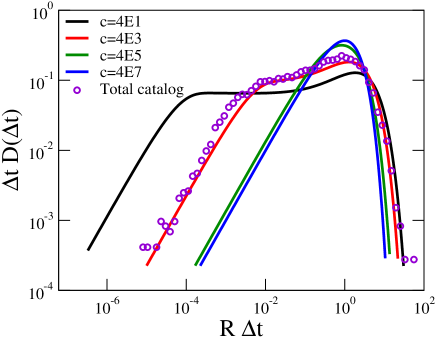
Figure 1: $\Delta tD(\Delta t)$ vs. $R\Delta t$ for the single Omori sequence with $\mu=3\cdot 10^{-7}$ events per second and varying $c$ from $40$ to $4\cdot 10^{7}$ sec (from left to right). Other model parameters are $T=1\cdot 10^{7}$ sec, $A=1$ and $p=1.05$. Open circles represent $\Delta tD(\Delta t)$ for the California catalog catalogo .

In Fig.2 we present the results of numerical simulations of the ETAS model obtained following the method of ref.hol . We perform extensive simulations in order to recover the limit $T\to\infty$ and neglect the dependence on $\mu T$. Previous studies hai have proposed that $D(\Delta t)$ only depends on the branching ratio and used this result to measure the ratio between triggered and independent events in experimental catalogs. Sornette et al. ss3 have shown that the functional form of $D(\Delta t)$ also depends on $p$, whose experimental values fluctuate around one. Our numerical simulations with a random $p\in]1,1.6]$ indicate that $D(\Delta t)$ depends on the average $p$ value. In the following we present result for simulations with $p=1.2$. A very similar pattern is obtained for other $p$ values. Fig. 2a shows that for fixed values of $\mu$ and $c$ the curves exhibit different behaviours for different ${\cal K}$, in agreement with previous results. We then focus on the role of the parameter $c$. In Fig. 2b, we plot $\Delta tD(\Delta t)$ at constant ${\cal K}$ and $c$ and for different values of $\mu$, as in ref.tou . We confirm the existence of deviations from scaling (1) at small $\Delta t$ which can be attributed to $c$. In order to show that the dependence on $c$ enters in the scaling form as $\mu\overline{c}$, in Fig. 2c, we fix the branching ratio ${\cal K}$ and vary $\mu$ as in Fig. 2b, but now $c$ is allowed to vary keeping constant $\mu c$. In this case all the distributions collapse on the same master curve revealing an ”universal” behaviour also at small $\Delta t$. This result indicates that deviations from Eq.(1) rely on the presence of the variable $\mu\overline{c}$ in Eq.(4). The dependence on this variable is relevant for $\Delta t<c$ and becomes negligible at larger $\Delta t$. This accounts for the appearance of deviations from universality only at small $\Delta t$.

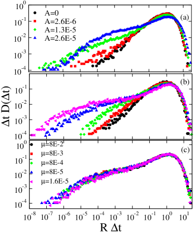
Figure 2: $\Delta tD(\Delta t)$ vs. $R\Delta t$ for the simulated catalogs with $T=10^{7}$ and $p=1.2$. (a) $\Delta tD(\Delta t)$ for $c=3000$, $\mu=8\cdot 10^{-6}$ events per unit time and varying ${\cal K}$ using different $A$ values reported in the legend. (b) $\Delta tD(\Delta t)$ for $c=3000$, ${\cal K}=0.5$ and varying $\mu$ according to the legend in panel (c). (c) We fix $c\mu=0.24$ obtaining data collapse with ${\cal K}=0.5$. In all figures the time unit is the iteration step of the model.

We now explore the role of the characteristic time $c$ on the scaling properties of $\Delta tD(\Delta t)$ for the experimental catalog catalogo . We first consider the whole catalog. In this case $\mu T$ is very large and does not affect the scaling form (5). To isolate the dependence on $\mu\overline{c}$, we plot $\Delta tD(\Delta t)$ including in the analysis only earthquakes above a lower magnitude thresholds $m_{th}$. $\mu/\overline{a}$, indeed, should not depend on $m_{th}$ ss2 and $\Delta tD(\Delta t)$ is expected to depend only on $R\Delta t$ and $\mu\overline{c}$. Fig.3a shows deviations from universality. Since these deviations are confined at small $\Delta t$ they are not easy to detect in the usual plot $R^{-1}D(\Delta t)$ vs $R\Delta t$ cor . Deviations must be attributed to $\mu\overline{c}$ and allow to identify $\overline{c}$ from the crossover points separating the linear growth from the plateau (identified by arrows in Fig.3a). Using the known values of $R$ we obtain that $\overline{c}$ is quite independent of $m_{th}$. This is consistent with $c_{i}$ independent of mainshock magnitudes but also with $c_{i}\propto 10^{\alpha(m_{i}-m_{th})}$ and $\alpha<b$ nota . The dependence of $c_{i}$ on $m_{i}$ and its influence on the $D(\Delta t)$ can be obtained by restricting the analysis to temporal periods soon after mainshocks. In these intervals, $\mu$ can be neglected simplifying the scaling relation (5). We further observe that for a single Omori sequence $R=N/T=a_{i}c_{i}\left[1-(T/c_{i})^{(1-p)}\right]/[T(p-1)]$ and therefore $R/a_{i}$ is a function only of the ratio $T/c_{i}$. In this case the scaling simplifies to

$$D(\Delta t)=RG_{2}\left(R\Delta t,\frac{T}{c_{i}}\right).$$ (6)

We start by considering the main-aftershock sequences for the three largest shocks recorded in the catalog: Landers, Northridge and Hector Mine. We consider as aftershocks all events with $m\geq 2.5$ occurring in a temporal window $[0,T]$ after the main event and within the aftershock zone, i.e. a radius $L=0.01\cdot 10^{0.5m_{i}}$km from the mainshock. Different definitions of the aftershock zone chris lead to very similar results. We first fix $T=10$ days for all sequences. In Fig. 3b the curves do not collapse but show a progressive shift as the mainshock magnitude increases. This effect can be attributed to dependence of $c_{i}$ on $m_{i}$. Therefore, at fixed $T$ the variable $T/c_{i}$ assumes different values for each sequence violating the collapse Eq.(1). As an alternative approach we use the criterion proposed in ref. bot to identify the end of a sequence: namely a sequence ends when the rate $\lambda(t)$ reaches the average Poisson rate $\mu\simeq 2$ events/day. Fig. 3c clearly indicates a very good data collapse for the different sequences in good agreement with Eq.(1). This can be understood from the scaling relation (6) where the variable $T/c_{i}$ assumes the same value for all sequences. Indeed, according to the Omori law, for $t\gg c$ the occurrence rate can be expressed as $\lambda(t)\sim 10^{\alpha m_{i}}t^{-p}$ and the condition $\lambda(T)=2$ provides $T\sim 10^{\alpha m_{i}/p}$. For the largest mainshocks, $c_{i}\sim 10^{bm_{i}/p}$ shc ; bot and therefore, the condition $\alpha\simeq b/p$ implies that the ratio $T/c_{i}$ is almost constant for the three sequences.

Next, we extend the above analysis to all sequences with mainshock magnitude $m>4$. To improve the statistics, we group mainshocks in classes of magnitude $m\in[M,M+0.5[$. Mainshocks are identified with the criterion suggested in ref.bot and the duration is again fixed by the condition $\mu(T)=2$. Other methods chris for aftershock identification provide similar results. Fig. 3d shows data collapse for all $M$ values. Since the criterion $\mu(T)=2$ roughly implies $T\sim 10^{\alpha M}$, the collapse of Fig. 3d, suggests that the dependence of $c_{i}$ on the mainshock magnitude as $c_{i}\sim 10^{bm_{i}/p}$ is valid also for intermediate mainshock magnitudes.

In conclusion, we address recent criticisms to the universal behaviour of the inter-event distribution. We follow the approach of ref.tou and show that $D(\Delta t)$ does exhibit universal features on the whole temporal range if four characteristic time scales are taken into account. In particular, deviations at small $\Delta t$ can be attributed to $c$ scaling differently from $\mu$. Whereas, by keeping constant $T/c$ for different sequences, the $D(\Delta t)$ collapse onto a unique master curve.

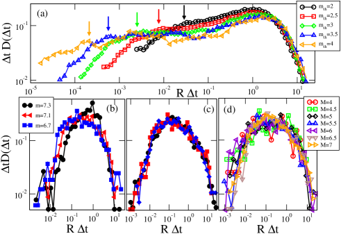
Figure 3: (a) $\Delta tD(\Delta t)$ vs. $R\Delta t$ for different magnitude thresholds $m_{th}$; (b) for the Landers, Northridge and Hector Mine sequences (mainshock magnitudes $m=7.3,6.7,7.1$, respectively) with fixed duration $T=10$ days; (c) for the Landers, Northridge and Hector Mine sequences with $T$ chosen following the criterion of ref.bot ; (d) for all sequences with a mainshock magnitude $m$ greater than 4 grouped in classes of $m$, $m\in[M,M+0.5[$.

References

- (1) P. Bak, K. Christensen, L. Danon, T. Scanlon , Phys. Rev. Lett. 88, 178501 (2002).
- (2) A. Corral, Phys. Rev. E 68, 035102(R) (2003).
- (3) A. Corral, Phys. Rev. Lett. 92, 108501 (2004).
- (4) A. Corral, Tectonophysics 424, 177 (2006).
- (5) R. Shcherbakov, G. Yakovlev, D. L. Turcotte, J. B. Rundle, Phys. Rev. Lett. 95, 218501 (2005).
- (6) M. Bottiglieri, E. Lippiello, C. Godano, L. de Arcangelis, J. Geophys. Res. 114, B03303 (2009).
- (7) M. Bottiglieri, C. Godano, L. D’Auria, J. Geophys. Res. 114, B10309 (2009).
- (8) J. Davidsen, C. Goltz, Geophys. Res. Lett. 31, L21612 (2004).
- (9) Molchan G.M., Pageoph 162, 1135 (2005);
- (10) S. Hainzl, C. Beauval, F. Scherbaum, Bull. Seismol. Soc. Am. 96, 313 (2006).
- (11) A. Saichev, D. Sornette, Phys. Rev. Lett. 97, 078501 (2006);
- (12) A. Saichev, D. Sornette, J. Geophys. Res. 112, B04313 (2007);
- (13) D. Sornette, S. Utkin, A. Saichev, Phys. Rev. E 77, 066109 (2008).
- (14) S. Touati, M. Naylor, I. G. Main, Phys. Rev. Lett. 102, 168501 (2009).
- (15) Y.Ogata, J. Am. Stat. Assoc. 83, 9 (1988).
- (16) C.A. Angell, Science 267, 1924 (1995); P. G. Debenedetti, F. H. Stillinger, Nature 410, 259 (2001); L. Cipelletti, L. Ramos, J. Phys.: Condens. Matter 17, R253 (2005).
- (17) M. Tarzia, A. Coniglio, Phys. Rev. Lett. 96, 075702 (2006); A. de Candia, E. Del Gado, A. Fierro and A. Coniglio, J. Stat. Mech., P02052 (2009); E. Del Gado, W. Kob, Phys. Rev. Lett. 98, 028303 (2007).
- (18) A. Helmstetter, Phys. Res. Lett. 91, 058501 (2003); A. Helmstetter, Y.Y. Kagan, D.D. Jackson, J. Geophys. Res. 110, B05S08 (2005); A. Helmstetter, Y.Y. Kagan, D.D. Jackson, Bull. Seism. Soc. Am. 96, 90 (2006).
- (19) R. Shcherbakov, D. L. Turcotte, J. B. Rundle, Geophys. Res. Lett. 31, L11613 (2004).
- (20) E. Lippiello, M. Bottiglieri, C. Godano, L. de Arcangelis, Geophys. Res. Lett. 34, L23301 (2007).
- (21) E. Lippiello, C. Godano, L. de Arcangelis, Phys. Rev. Lett. 98, 098501 (2007).
- (22) E. Lippiello, L. de Arcangelis, C. Godano, Phys. Rev. Lett. 100, 038501 (2008).
- (23) E. Lippiello, L. de Arcangelis, C. Godano, Phys. Rev. Lett. 103, 038501 (2009).
- (24) Y.Y. Kagan, Bull. Seism. Soc. Am. 94, 1207 (2004).
- (25) T. Utsu, International Handbook of Earthquake and Engineering Seismology 81A, 719 (2002).
- (26) We analyze the relocated California catalog in the years 1981-2005, in the region south (north) latitude 31 (38), west (east) longitude 121 (113), for magnitudes larger than . P. Shearer, E. Hauksson, G. Lin, Bull. Seismol. Soc. Am. 95, 904 (2005).
- (27) J. R. Holliday, D. L. Turcotte, J. B. Rundle, Pure appl. geophys. 165, 1003 (2008).
- (28) . Using we obtain .
- (29) A. Christophersen, E.G.C. Smith, Bull. Seismol. Soc. Am. 98, 2133 (2008).