Cooper pairing and BCS-BEC evolution in mixed-dimensional Fermi gases

Abstract

Similar to what has recently been achieved with Bose-Bose mixtures lamporesi , mixed-dimensional Fermi-Fermi mixtures can be created by applying a species-selective one-dimensional optical lattice to a two-species Fermi gas ($\sigma\equiv\{\uparrow,\downarrow\}$), such a way that both species are confined to quasi-two-dimensional geometries determined by their hoppings along the lattice direction. We investigate the ground state phase diagram of superfluidity for such mixtures in the BCS-BEC evolution, and find normal, gapped superfluid, gapless superfluid, and phase separated regions. In particular, we find a stable gapless superfluid phase where the unpaired $\uparrow$ and $\downarrow$ fermions coexist with the paired (or superfluid) ones in different momentum space regions. This phase is in some ways similar to the Sarma state found in mixtures with unequal densities, but in our case, the gapless superfluid phase is unpolarized and most importantly it is stable against phase separation.

I Introduction

Atomic Fermi gases have emerged as unique testing ground for many theories of exotic matter in nature, allowing for the creation of complex yet very controllable many-body quantum systems review , where for instance observation of the BCS-BEC crossover has so far been the most important achievement in this field. Following this huge success with single-species fermion mixtures, there has been increasing experimental interest in studying two-species Fermi-Fermi mixtures taglieber08 ; wille08 ; voigt09 ; spiegelhalder09 ; tiecke09 ; spiegelhalder10 . In particular, ⁶Li-⁴⁰K mixtures have recently been trapped and interspecies Feshbach resonances have been identified, opening a new frontier in ultracold atom research to study exotic many-body phenomena, one of which is the possibility of studying fermion pairing in mixed dimensions nishida08 ; nishida09 ; nishida10 .

Mixed-dimensional atomic systems, in which two types of particles live in different dimensions, can be created with two-species Fermi-Fermi, Bose-Fermi, and Bose-Bose mixtures by using species-selective optical lattice potentials. This has recently been achieved with Bose-Bose mixtures lamporesi by applying a one-dimensional optical lattice to the ⁴¹K-⁸⁷Rb mixture, where only ⁴¹K atoms feel the lattice potential, and they are confined to a quasi-two-dimensional geometry, while having negligible effect on ⁸⁷Rb atoms, that is leaving ⁸⁷Rb atoms three dimensional. Motivated by this experimental work, here we analyze Cooper pairing in mixed-dimensional Fermi gases. We consider both single-species and two-species fermion mixtures, and analyze the ground state phase diagrams in the BCS-BEC evolution, which involves normal, gapped superfluid, gapless superfluid, and phase separated regions. In particular, the gapless superfluid phase, where the unpaired $\uparrow$ and $\downarrow$ fermions coexist with the paired (or superfluid) ones in different momentum space regions, is in some ways similar to the Sarma state found in mixtures with unequal densities sarma , but in our case, the gapless superfluid phase is unpolarized and most importantly it is stable against phase separation. In this way, our gapless superfluid phase is very similar to those of Refs. eite ; feigun , which are recently proposed for ultracold atomic systems in other contexts.

The rest of the manuscript is organized as follows. In Sec. II, after introducing the Hamiltonian in Sec. II.1, the corresponding saddle-point self-consistency equations are derived in Sec. II.2, and their noninteracting limit is discussed in Sec. II.3. We numerically solve these equations in the BCS-BEC evolution in Sec. III, where we investigate the normal-superfluid transition in Sec. III.1, the topological gapless-gapped superfluidity transition in Sec. III.2, and the ground state phase diagrams in Sec. III.3. A brief summary of our conclusions is given in Sec. IV. We also include three appendices, where the self-consistency equations are further discussed in Appendix A, boundary equation for the normal-superfluid transition is derived in Appendix B, and the molecular BEC limit is investigated in Appendix C.

II Mixed-dimensional Fermi gases

In this work, we analyze Cooper pairing in mixed-dimensional Fermi gases, which seems to be a very promising way to create superfluidity with mismatched Fermi surfaces, and the physics involved is in some ways similar to that of the unequal density mixtures zwierlerin06 ; partridge06 ; shin08 ; salomon10 . We consider only uniform (homogenous) mixtures, but emphasize that the finite-size effects due to the confining trapping potentials (which are always present in atomic systems) can be taken into account using the local-density approximation (as a first approximation).

II.1 Hamiltonian

To describe such mixed-dimensional Fermi gases in a species-selective one-dimensional optical lattice (say in the $\mathbf{\widehat{z}}$ direction), we start with the real-space Hamiltonian ($\hbar=k_{B}=1$)

$$H =\sum_{\sigma}\int d^{3}\mathbf{r}\psi_{\mathbf{r},\sigma}^{\dagger}\left[-\frac{\nabla^{2}}{2m_{\sigma}}-\mu_{\sigma}+V_{OL}^{\sigma}(r_{z})\right]\psi_{\mathbf{r},\sigma}$$

$$-g\int d^{3}\mathbf{r}\psi_{\mathbf{r},\uparrow}^{\dagger}\psi_{\mathbf{r},\downarrow}^{\dagger}\psi_{\mathbf{r},\downarrow}\psi_{\mathbf{r},\uparrow},$$ (1)

where the pseudo-spin $\sigma$ labels both the type and hyperfine states of atoms represented by the creation operator $\psi_{\mathbf{r},\sigma}^{\dagger}$, and $m_{\sigma}$ is the mass and $\mu_{\sigma}$ is the chemical potential. Here, $\mathbf{r}\equiv(r_{x},r_{y},r_{z})$ is the position with $r_{\perp}=\sqrt{r_{x}^{2}+r_{y}^{2}}$, $V_{OL}^{\sigma}=V_{0,\sigma}\sin^{2}(\pi r_{z}/d_{z})$ is the optical lattice potential, $d_{z}$ is the lattice spacing, and $g\geq 0$ is the strength of the attractive interaction (zero-range and isotropic) between $\uparrow$ and $\downarrow$ fermions.

In order to achieve the momentum-space Hamiltonian, we first expand the creation and annihilation field operators in the orthonormal and complete basis set of Wannier functions $W(r_{z}-r_{z}^{i})$ of the lowest-energy states of the optical potential near their minima (single-band approximation), and then take the Fourier transform of the site operators. This corresponds to the following substitution: $\psi_{\mathbf{r},\sigma}=(1/\sqrt{M})\sum_{i,\mathbf{k}}a_{\mathbf{k},\sigma}W_{\sigma}(r_{z}-r_{z}^{i})e^{-i(\mathbf{k_{\perp}}\cdot\mathbf{r_{\perp}}+k_{z}r_{z}^{i})},$ where $\mathbf{k}\equiv(k_{x},k_{y},k_{z})$ is the momentum with $k_{\perp}=\sqrt{k_{x}^{2}+k_{y}^{2}}$, $i$ labels the lattice sites, and $M$ is the total number of them. Keeping only the tunneling between nearest-neighbor sites and onsite interactions, and using the orthonormality of the Wannier functions, the resultant Hamiltonian can be written as

$$H=\sum_{\mathbf{k},\sigma}\xi_{\mathbf{k},\sigma}a_{\mathbf{k},\sigma}^{\dagger}a_{\mathbf{k},\sigma}-g\sum_{\mathbf{k},\mathbf{k^{\prime}},\mathbf{q}}b_{\mathbf{k},\mathbf{q}}^{\dagger}b_{\mathbf{k^{\prime}},\mathbf{q}},$$ (2)

where $b_{\mathbf{k},\mathbf{q}}^{\dagger}=a_{\mathbf{k}+\mathbf{q}/2,\uparrow}^{\dagger}a_{-\mathbf{k}+\mathbf{q}/2,\downarrow}^{\dagger}$ creates fermion pairs with center of mass momentum $\mathbf{q}$ and relative momentum $2\mathbf{k}$. Here, $\xi_{\mathbf{k},\sigma}=\epsilon_{\mathbf{k},\sigma}-\mu_{\sigma},$ where $\epsilon_{\mathbf{k},\sigma}=k_{\perp}^{2}/(2m_{\sigma})+2t_{\sigma}\left[1-\cos(k_{z}d_{z})\right]$ is the single-particle energy dispersion, and $t_{\sigma}=\int dr_{z}W^{*}(r_{z}-r_{z}^{i})\left[-\partial^{2}/(2m_{\sigma}\partial r_{z}^{2})+V_{OL}^{\sigma}(r_{z})\right]W(r_{z}-r_{z}^{j})$ is the tunneling amplitude between any nearest-neighbor sites $i$ and $j$.

Following the usual treatment, strength of the attractive interaction can be written in terms of an “effective” $s$-wave scattering length $a_{eff}$ as $1/g=-m_{+}V/(4\pi a_{eff})+\sum_{\mathbf{k}}1/(2\epsilon_{\mathbf{k},+}),$ where $m_{\pm}=2m_{\uparrow}m_{\downarrow}/(m_{\downarrow}\pm m_{\uparrow}),$ $V$ is the volume of the system, and $\epsilon_{\mathbf{k},\pm}=(\epsilon_{\mathbf{k},\uparrow}\pm\epsilon_{\mathbf{k},\downarrow})/2.$ Note that $m_{+}$ is twice the reduced mass of the $\uparrow$ and $\downarrow$ fermions, and that the equal mass case corresponds to $|m_{-}|\to\infty$. Here, and throughout, the momentum space sums are evaluated as $\sum_{\mathbf{k}}\equiv[V/(2\pi)^{3}]\int d^{3}\mathbf{k}\equiv[V/(2\pi^{2})]\int_{0}^{\pi/d_{z}}dk_{z}\int_{0}^{\infty}k_{\perp}dk_{\perp},$ since the system at hand has a cylindrical symmetry around the $k_{z}$-axis, and a translational symmetry along the $\mathbf{\widehat{z}}$ direction, so that the $k_{z}$ integrals are limited to the first Brillouin zone, i.e. $-\pi/d_{z}\leq k_{z}\leq\pi/d_{z}$. The resultant integrands are also even functions of $k_{z}$, and hence we integrate over half of the Brillouin zone and multiply them by two.

In this manuscript, for its simplicity, we set $t_{\downarrow}=1/(2m_{\downarrow}d_{z}^{2})$ but allow for the $\uparrow$ fermions to have a different effective mass along the lattice direction through a tight-binding dispersion determined by $t_{\uparrow}$, so that

$$\epsilon_{\mathbf{k},\uparrow} = \frac{k_{\perp}^{2}}{2m_{\uparrow}}+2t_{\uparrow}\left[1-\cos(k_{z}d_{z})\right],$$ (3)

$$\epsilon_{\mathbf{k},\downarrow} = \frac{k_{\perp}^{2}}{2m_{\downarrow}}+\frac{1}{m_{\downarrow}d_{z}^{2}}\left[1-\cos(k_{z}d_{z})\right].$$ (4)

Notice that when $k_{Fz,\downarrow}d_{z}\ll\pi$ (i.e. the low-filling limit for the $\downarrow$ species), where $k_{Fz,\downarrow}$ is the Fermi momentum of $\downarrow$ fermions in the $k_{z}$ direction, since Eq. (4) can be approximated as $\epsilon_{\mathbf{k},\downarrow}\approx k^{2}/(2m_{\downarrow})$, optical lattice has negligibe effect on $\downarrow$ fermions in this limit. Next, we analyze the phase diagram of the Hamiltonian given in Eq. (2) with the dispersions given by Eqs. (3) and (4), within the saddle-point (mean-field) approximation.

II.2 Self-consistency equations

At low temperatures ($T\approx 0$), the saddle-point self-consistency (order parameter and number) equations are sufficient to describe the BCS-BEC evolution of superfluidity leggett ; jan . For the Hamiltonian given in Eq. (2), the saddle-point action is $S_{0}=\Omega_{0}/T$, where

$$\Omega_{0}=\frac{|\Delta|^{2}}{g}+\sum_{\mathbf{k}}\left(\xi_{\mathbf{k},+}-E_{\mathbf{k},+}\right)+T\sum_{\mathbf{k},s}\ln[f(-E_{\mathbf{k},s})]$$ (5)

is the saddle-point thermodynamic potential. Here, $f(x)=1/[\exp(x/T)+1]$ is the Fermi function, $E_{\mathbf{k},s}=(\xi_{\mathbf{k},+}^{2}+|\Delta|^{2})^{1/2}+\gamma_{s}\xi_{\mathbf{k},-}$ is the quasiparticle energy when $\gamma_{1}=1$ or the negative of the quasihole energy when $\gamma_{2}=-1$, and $E_{\mathbf{k},\pm}=(E_{\mathbf{k},1}\pm E_{\mathbf{k},2})/2.$ In addition, $\Delta$ is the order parameter and $\xi_{\mathbf{k},\pm}=\epsilon_{\mathbf{k},\pm}-\mu_{\pm},$ where $\mu_{\pm}=(\mu_{\uparrow}\pm\mu_{\downarrow})/2.$ Note that the symmetry between quasiparticles and quasiholes is broken when $\xi_{\mathbf{k},-}\neq 0$.

The saddle-point condition $\delta\Omega_{0}/\delta\Delta^{*}=0$ leads to an equation for the order parameter,

$$-\frac{m_{+}V}{4\pi a_{eff}}=\sum_{\mathbf{k}}\left[\frac{1-f(E_{\mathbf{k},1})-f(E_{\mathbf{k},2})}{2E_{\mathbf{k},+}}-\frac{1}{2\epsilon_{\mathbf{k},+}}\right],$$ (6)

where, as usual, $g$ is eliminated in favor of the effective $s$-wave scattering length $a_{eff}$ via the relation given above leggett ; jan . The order parameter equation has to be solved self-consistently with the number equations. At the saddle point, the relation $N_{\sigma}=-\partial\Omega_{0}/\partial{\mu_{\sigma}}$ leads to

$$N_{\uparrow} = \sum_{\mathbf{k}}\left[|u_{\mathbf{k}}|^{2}f(E_{\mathbf{k},1})+|v_{\mathbf{k}}|^{2}f(-E_{\mathbf{k},2})\right],$$ (7)

$$N_{\downarrow} = \sum_{\mathbf{k}}\left[|u_{\mathbf{k}}|^{2}f(E_{\mathbf{k},2})+|v_{\mathbf{k}}|^{2}f(-E_{\mathbf{k},1})\right],$$ (8)

where $|u_{\mathbf{k}}|^{2}=(1+\xi_{\mathbf{k},+}/E_{\mathbf{k},+})/2$ and $|v_{\mathbf{k}}|^{2}=(1-\xi_{\mathbf{k},+}/E_{\mathbf{k},+})/2$ are the usual coherence factors. At $T=0$, Eqs. (6), (7) and (8) can be simplified considerably as shown in Appendix A.

In order to analyze the phase diagram at $T=0$, we solve the saddle-point self-consistency equations and check the stability of these solutions for the uniform superfluid phase using the compressibility (or the curvature) criterion iskin06 ; he06 ; pao06 . This says that the compressibility matrix $\mathbf{\kappa}(T)$ with elements $\kappa_{\sigma,\sigma^{\prime}}(T)=-\partial^{2}\Omega_{0}/(\partial\mu_{\sigma}\partial\mu_{\sigma^{\prime}})$ needs to be positive definite, and it is related (identical) to the condition that the curvature

$$\frac{\partial^{2}\Omega_{0}}{\partial\Delta^{2}}=|\Delta|^{2}\sum_{\mathbf{k},s}\left[\frac{0.5-f(E_{\mathbf{k},s})}{E_{\mathbf{k},+}^{3}}+\frac{f^{\prime}(E_{\mathbf{k},s})}{E_{\mathbf{k},+}^{2}}\right]$$ (9)

of the saddle-point thermodynamic potential $\Omega_{0}$ with respect to the saddle-point parameter $\Delta$ needs to be positive. Here, $f^{\prime}(x)=df(x)/dx$. When at least one of the eigenvalues of $\mathbf{\kappa}(T)$, or the curvature $\partial^{2}\Omega_{0}/\partial\Delta^{2}$ is negative, the uniform saddle-point solution does not correspond to a minimum of $\Omega_{0}$, and a nonuniform superfluid phase, e.g. a phase separation, is favored.

II.3 Noninteracting Limit

Before presenting our numerical results, let’s first analyze the noninteracting $g\to 0$ limit. In this limit, since $1/a_{eff}\to-\infty$, the order parameter vanishes $\Delta\to 0$, and at $T=0$ Eqs. (7) and (8) can be written as $N_{\sigma}=\sum_{\mathbf{k}}\theta(-\xi_{\mathbf{k},\sigma}),$ where $\theta(x)$ is the heaviside step function. Evaluating the $\mathbf{k}$-space sums, the density $n_{\sigma}=N_{\sigma}/V$ of the $\sigma$ fermions become

$$n_{\sigma} = \frac{m_{\sigma}k_{Fz,\sigma}}{2\pi^{2}}(\mu_{\sigma}-2t_{\sigma})+\frac{m_{\sigma}t_{\sigma}}{\pi^{2}d_{z}}\sin(k_{Fz,\sigma}d_{z}),$$ (10)

$$\mu_{\sigma} = 2t_{\sigma}\left[1-\cos(k_{Fz,\sigma}d_{z})\right],$$ (11)

where $k_{Fz,\sigma}\geq 0$ corresponds to the Fermi momentum of the $\sigma$ fermions in the $k_{z}$ direction, which is related to the chemical potential via Eq. (11).

Note that, in the low-density ($k_{Fz,\downarrow}d_{z}\ll\pi$) limit, expanding out Eqs. (10) and (11) to the lowest nontrivial orders (third and second orders, respectively) in $k_{Fz,\downarrow}d_{z}$, we obtain $n_{\downarrow}\approx m_{\downarrow}k_{Fz,\downarrow}(\mu_{\downarrow}-t_{\downarrow}k_{Fz,\downarrow}^{3}d_{z}^{2}/3)/(2\pi^{2})$ and $\mu_{\downarrow}\approx t_{\downarrow}k_{Fz,\downarrow}^{2}d_{z}^{2}$. Combining these two expressions, and setting $k_{Fz,\downarrow}=k_{F,\downarrow}$ or $t_{\downarrow}=1/(2m_{\downarrow}d_{z}^{2})$, the density of $\downarrow$ fermions acquires the usual form $n_{\downarrow}\approx k_{F,\downarrow}^{3}/(6\pi^{2}).$ In addition, when $t_{\uparrow}\to 0$ and $k_{Fz,\uparrow}=\pi/d_{z}$, Eq. (10) reduces to the density of $\uparrow$ fermions in each (isolated) two-dimensional planes along the $k_{z}$ direction, $N_{\uparrow}/(MA)=m_{\uparrow}k_{F,\uparrow}^{2}/(4\pi),$ which is of the usual form, where we used $V=AL_{z}$ with $A$ being the area of the system in the $(x,y)$ plane and $L_{z}$ is the system size in the $\mathbf{\widehat{z}}$ direction. Here, $M=L_{z}/d_{z}$ is the number of two-dimensional planes, i.e. the number of lattice sites, in the $\mathbf{\widehat{z}}$ direction. Having discussed the noninteracting limit, next we analyze the BCS-BEC evolution.

III Saddle-point Approximation

In this section, we consider only equal density mixtures, where $n_{\uparrow}=n_{\downarrow}$, at zero temperature. For these mixtures, first we analyze the amplitude of the order parameter $|\Delta|$, chemical potential sum $\mu_{+}$, and the chemical potential difference $\mu_{-}$ as a function of the tunneling amplitude $t_{\uparrow}$ and effective scattering length $1/(k_{F,\downarrow}a_{eff})$ for fixed values of $k_{F,\downarrow}d_{z}$. Here, $k_{F,\downarrow}$ is an “effective” Fermi momentum for $\downarrow$ fermions defined through the three-dimensional density $n_{\downarrow}=k_{F,\downarrow}^{3}/(6\pi^{2})$, where $n_{\downarrow}$ is given by Eq. (10). Then, using the stability criterion given in Eq. (9), we construct the phase diagrams. For its simplicity, we mainly present our results for the equal mass ($m_{\uparrow}=m_{\downarrow}$) mixtures, but we also briefly mention the effects of mass anisotropy $m_{\uparrow}\neq m_{\downarrow}$ on the phase diagrams.

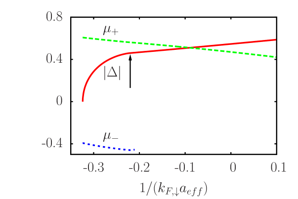
Figure 1: (Color online) Saddle-point solutions for the amplitude of the order parameter $|\Delta|$, chemical potential sum $\mu_{+}=(\mu_{\uparrow}+\mu_{\downarrow})/2$, and the chemical potential difference $\mu_{-}=(\mu_{\uparrow}-\mu_{\downarrow})/2$ are shown (in units of $\epsilon_{F,\downarrow}$) as a function of the effective $s$-wave scattering parameter $1/(k_{F,\downarrow}a_{eff})$. ($\mu_{-}$ is shown only for weak interactions where it is relevant). This data corresponds to the case where $m_{\uparrow}=m_{\downarrow}$, $t_{\uparrow}=\epsilon_{F,\downarrow}$ and $k_{F,\downarrow}d_{z}=0.1$. The arrow shows the location of the topological gapless superfluid to gapped superfluid transition discussed in the text.

III.1 Normal-Superfluid transition

Using $k_{F,\downarrow}$ and $\epsilon_{F,\downarrow}=k_{F,\downarrow}^{2}/(2m_{\downarrow})$ as our length and energy scales, respectively, we solve Eqs. (12), (13) and (14) numerically. For instance, in Fig. 1, we show self-consistent solutions of $|\Delta|$, $\mu_{+}$ and $\mu_{-}$ as a function of $1/(k_{F,\downarrow}a_{eff})$, when $m_{\uparrow}=m_{\downarrow}$, $t_{\uparrow}=\epsilon_{F,\downarrow}$ and $k_{F,\downarrow}d_{z}=0.1$. When the scattering parameter is smaller than a critical value, i.e. $1/(k_{F,\downarrow}a_{eff})\lesssim-0.32$, the saddle-point solution $\mu_{\downarrow}=\mu_{+}-\mu_{-}\to 1$ (in units of $\epsilon_{F,\downarrow}$) since $|\Delta|=0$, indicating that the mixture is a normal Fermi gas nishidanote . Beyond this critical value, the superfluid order parameter $|\Delta|$ becomes nonzero indicating a quantum phase transition from the normal to a superfluid phase.

This transition can be understood from earlier works on Cooper pairing with mismatched Fermi surfaces. For instance, in the case of Fermi gases with unequal densities in purely three-dimensions, a superfluid to normal phase transition has been recently observed beyond a critical density difference depending on the value of the scattering parameter zwierlerin06 ; partridge06 ; shin08 ; salomon10 . This transition occurs when the difference in the chemical potentials (or Fermi momenta) reaches what is known as the Clogston-Chandrasekhar limit clogston ; chandrasekhar . In our case, the main mechanism is the same. As can be extracted from Eq. (11), the mismatch is inevitable in some parts of the $\mathbf{k}$-space even for the equal density mixtures considered in this manuscript. Therefore, it is energetically more favorable for the mixture to be in the normal phase until a critical scattering parameter is reached, beyond which Cooper pairing is possible.

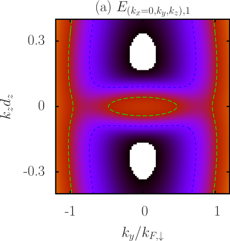
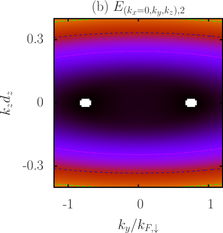
Figure 2: (Color online) Contour maps of (a) the quasiparticle excitation energy $E_{\mathbf{k},1}$, and (b) the negative of the quasihole excitation energy $E_{\mathbf{k},2}$ are shown as a function of momentum components $k_{z}$ (in units of $1/d_{z}$) and $k_{y}$ (in units of $k_{F,\downarrow}$) in the $k_{x}=0$ plane. This data corresponds to the case where $m_{\uparrow}=m_{\downarrow}$, $t_{\uparrow}=\epsilon_{F,\downarrow}$, $k_{F,\downarrow}d_{z}=0.1$ and $1/(k_{F,\downarrow}a_{eff})=-0.25$. The excitations are gapless ($E_{\mathbf{k},s}\leq 0$) in the white regions.

III.2 Topological gapless-gapped superfluidity transition

With further increase in the scattering parameter, $|\Delta|$ increases quite rapidly and $\mu_{+}$ decreases, with a kink in the former quantity at $1/(k_{F,\downarrow}a_{eff})\approx-0.22$. (We also expect a weak kink in $\mu_{+}$ at the same point, but it is not clearly seen in the data.) Therefore, the BCS-BEC evolution in mixed-dimensional Fermi gases is nonanalytic, i.e. it is not a crossover. Recall that, in usual three-dimensional mixtures, the evolution of $|\Delta|$ and $\mu_{+}$ is analytic for all $1/(k_{F,\downarrow}a_{eff})$, and the evolution is just a crossover. The kink in $|\Delta|$ is more pronounced for lower values of $t_{\uparrow}$, and it signals a topological quantum phase transition as discussed next.

The excitation spectrum of quasiparticles are determined by energies $E_{\mathbf{k},1}$ and $E_{\mathbf{k},2}$. At $\mathbf{k}$-space points, the condition $E_{\mathbf{k},s}=0$ defines Fermi surfaces of quasiparticles in momentum space where the quasiparticle excitation spectrum changes from a gapped to a gapless phase. These changes in the Fermi surfaces of quasiparticles are topological in nature volovik , and we identify topological quantum phase transitions associated with the disappearance or appearance of momentum space regions of zero quasiparticle energies when either $1/(k_{F,\downarrow}a_{eff})$, $t_{\uparrow}$, and/or $k_{F,\downarrow}d_{z}$ is changed. Note that the topological transition occurs without changing the symmetry of the order parameter as the Landau classification demands for ordinary phase transitions.

We illustrate the gapless superfluid phase in Fig. 2, where contour maps of $E_{\mathbf{k},s}$ are shown as a function of $k_{z}$ and $k_{y}$ in the $k_{x}=0$ plane, when $m_{\uparrow}=m_{\downarrow}$, $t_{\uparrow}=\epsilon_{F,\downarrow}$, $k_{F,\downarrow}d_{z}=0.1$ and $1/(k_{F,\downarrow}a_{eff})=-0.25$. In Fig. 1, this data corresponds to a point that is slightly on the left hand side of the transition point indicated by an arrow. The excitations are gapless ($E_{\mathbf{k},s}\leq 0$) in the white regions.

The topological transition could be potentially observed through the measurement of the momentum distribution $n_{\mathbf{k},\sigma}$ of the fermions md , which can be extracted from Eqs. (7) and (8). For $\mathbf{k}$-space regions where $E_{{\bf k},1}>0$ and $E_{\mathbf{k},2}>0$, the corresponding momentum distributions are equal $n_{\mathbf{k},\uparrow}=n_{\mathbf{k},\downarrow}$. However, when $E_{\mathbf{k},1}\leq 0$ and $E_{\mathbf{k},2}>0$, then $n_{\mathbf{k},\uparrow}=1$ and $n_{\mathbf{k},\downarrow}=0$. Similarly, when $E_{\mathbf{k},1}>0$ and $E_{\mathbf{k},2}\leq 0$, then $n_{\mathbf{k},\uparrow}=0$ and $n_{\mathbf{k},\downarrow}=1$. We illustrate these cases in Fig. 3 for the parameters of Fig. 2. Note that, although there are excess (or unpaired) $\uparrow$ or $\downarrow$ fermions in different regions of the $\mathbf{k}$-space, i.e. the bright yellow regions, there are equal number of $\uparrow$ and $\downarrow$ fermions in total. The size of yellow regions may look very different in (a) and (b) due partly to the difference in scaling factors in $k_{z}$ and $k_{y}$.

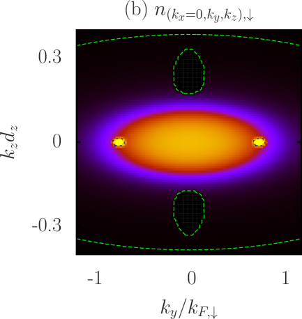
Figure 3: (Color online) Contour maps of the momentum distributions (a) $n_{\mathbf{k},\uparrow}$ for the $\uparrow$ fermions, and (b) $n_{\mathbf{k},\downarrow}$ for the $\downarrow$ fermions are shown as a function of momentum components $k_{z}$ (in units of $1/d_{z}$) and $k_{y}$ (in units of $k_{F,\downarrow}$) in the $k_{x}=0$ plane. This data corresponds to the case considered in Fig. 2, where $m_{\uparrow}=m_{\downarrow}$, $t_{\uparrow}=\epsilon_{F,\downarrow}$, $k_{F,\downarrow}d_{z}=0.1$ and $1/(k_{F,\downarrow}a_{eff})=-0.25$. Note that when $E_{{\bf k},1}>0$ and $E_{\mathbf{k},2}>0$, then $n_{\mathbf{k},\uparrow}=n_{\mathbf{k},\downarrow}$. However, when $E_{\mathbf{k},1}\leq 0$ and $E_{\mathbf{k},2}>0$, then $n_{\mathbf{k},\uparrow}=1$ and $n_{\mathbf{k},\downarrow}=0$; and when $E_{\mathbf{k},1}>0$ and $E_{\mathbf{k},2}\leq 0$, then $n_{\mathbf{k},\uparrow}=0$ and $n_{\mathbf{k},\downarrow}=1$. The densities are 1 (0) in the bright yellow (black) regions.

This topological transition is quantum ($T=0$) in nature, but its signatures should still be observed at finite temperatures within the quantum critical region, where the momentum distributions are smeared out due to thermal effects. In addition, while thermodynamic quantities such as atomic compressibility, specific heat, and spin susceptibility have power-law dependences on the temperature in the BCS side, they have exponential dependences on the temperature and the minimum energy of quasiparticle excitations in the BEC side, again signaling the existence of a quantum phase transition at $T=0$. Having discussed the topological classification of possible superfluid phases, we are ready to present the saddle-point phase diagrams at $T=0$, including the stability analysis (positive curvature criterion) of the solutions.

III.3 Ground state phase diagrams

In Fig. 4, ground state phase diagrams are shown as a function of the tunneling amplitude $t_{\uparrow}$ and the effective $s$-wave scattering parameter $1/(k_{F,\downarrow}a_{eff})$ for fixed values of (a) $k_{F,\downarrow}d_{z}=0.1$, and (b) $k_{F,\downarrow}d_{z}=1$. We indicate normal ($N$), gapped uniform superfluid ($SF$), gapless uniform superfluid ($gSF$), and phase-separated ($PS$) regions. The normal phase is characterized by a vanishing order parameter ($\Delta=0$), while the gapped superfluid and gapless superfluid phases are both characterized by $\Delta>0$ and $\partial^{2}\Omega_{0}/\partial\Delta^{2}>0$, but with distinct $\mathbf{k}$-space topologies as discussed above. In the $gSF$ phase, the unpaired $\uparrow$ and $\downarrow$ fermions coexist with the paired (or superfluid) ones in different $\mathbf{k}$-space regions, but there are no unpaired fermions in the $SF$ phase, i.e. all $\uparrow$ and $\downarrow$ fermions are paired. The $gSF$ phase is in some ways similar to the Sarma state found in mixtures with unequal densities sarma , but in our case, the gapless superfluid phase is unpolarized and most importantly it is stable against phase separation. The phase-separated region is characterized by $\partial^{2}\Omega_{0}/\partial\Delta^{2}<0$, but this region could also be of the FFLO-type superfluid having spatial modulations FF ; LO . Such a possibility is not considered in this manuscript, and it is left as an important problem to address in the future.

We can understand these phase diagrams as follows. For a fixed $t_{\uparrow}$, when the scattering parameter is smaller than a critical value, the potential energy is not sufficient to cause pairing due to mismatch of the Fermi surfaces, and the mixture is a normal Fermi gas with $\Delta=0$. As shown in Fig. 4(a), the critical scattering parameter decreases with increasing $t_{\uparrow}$, since increasing $t_{\uparrow}$ decreases the mismatch for lower values of $t_{\uparrow}$. In the normal region, when $t_{\uparrow}=0$, Fermi surface of the $\uparrow$ fermions is a cylindrical shell in the $\mathbf{k}$-space with height $k_{Fz,\uparrow}=2\pi/d_{z}$ and radius $k_{F,\uparrow}$. However, in the low-filling limit of $\downarrow$ fermions, Fermi surface of the $\downarrow$ fermions is more like a spherical shell with radius $k_{F,\downarrow}$. Note that for equal mass and equal density mixtures considered here, the $\mathbf{k}$-space volumes enclosed by the cylindrical and spherical Fermi surfaces must be equal. Therefore, at $t_{\uparrow}=0$, there is a large mismatch between the two Fermi surfaces when $k_{F,\uparrow}\ll k_{F,\downarrow}\ll\pi/d_{z}$, and increasing $t_{\uparrow}$ from zero decreases $k_{Fz,\uparrow}$ and increases the ratio $k_{F,\uparrow}/k_{F,\downarrow}$. When this happens, Fermi surface of the $\uparrow$ fermions looks like a prolate spheroid (like an american football). This decreases the mismatch for small values of $t_{\uparrow}$ as long as $k_{F,\uparrow}\lesssim k_{F,\downarrow}$, and it is qualitatively what happens along the normal-superfluid transition boundary in Fig. 4(a), when $k_{F,\downarrow}d_{z}=0.1\ll\pi$.

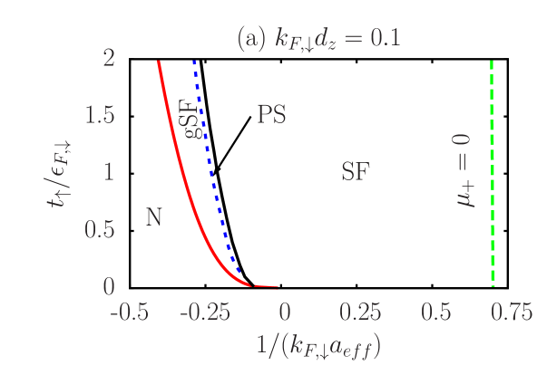
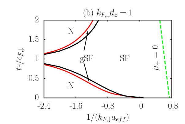
Figure 4: (Color online) Ground state phase diagrams are shown as a function of the tunneling amplitude $t_{\uparrow}$ (in units of $\epsilon_{F,\downarrow}$) and the effective $s$-wave scattering parameter $1/(k_{F,\downarrow}a_{eff})$. Here, we consider equal density ($n_{\uparrow}=n_{\downarrow}$) and equal mass ($m_{\uparrow}=m_{\downarrow}$) mixtures, for fixed values of $k_{F,\downarrow}d_{z}=0.1$ in (a), and $k_{F,\downarrow}d_{z}=1$ in (b). We show normal ($N$), gapped uniform superfluid ($SF$), gapless uniform superfluid ($gSF$), and phase-separated ($PS$) regions. The $PS$ region in (b) is close to the normal-superfluid transition boundary, but it is very small and not shown. There is no phase transition across $\mu_{+}=0$ (green-dashed) line, it is only shown as a reference point.

In Fig. 4(b), we show the same phase diagram for a higher value of $k_{F,\downarrow}d_{z}=1$. Similar to Fig. 4(a), the critical scattering parameter for the normal-superfluid transition decreases initially with increasing $t_{\uparrow}$, since increasing $t_{\uparrow}$ decreases the mismatch for lower values of $t_{\uparrow}$. In contrast, beyond a critical value of $t_{\uparrow}$ [e.g. $t_{\uparrow}\gtrsim\epsilon_{F,\downarrow}$ in Fig. 4(b)], the critical scattering parameter increases with increasing $t_{\uparrow}$. This is because, since increasing $t_{\uparrow}$ decreases $k_{F,z}$ and increases the ratio $k_{F,\uparrow}/k_{F,\downarrow}$, it eventually increases the mismatch of the two Fermi surfaces after $k_{F,\uparrow}>k_{F,\downarrow}$. When this happens, the Fermi surface of the $\uparrow$ fermions changes from a prolate spheroid to an oblate spheroid (a disk-shaped ellipsoid). For the case considered in Fig. 4(a) where $k_{F,\downarrow}d_{z}=0.1$, we found that this occurs beyond $t_{\uparrow}\gtrsim 100\epsilon_{F,\downarrow}$, but it is not shown. In general, for equal mass and equal density mixtures, such a change is expected to occur beyond $t_{\uparrow}\gtrsim 1/(2m_{\uparrow}d_{z}^{2})$, and this expectation is consistent with our numerical findings.

In addition, in Fig. 4, the solid-black lines correspond to the transition boundary between the gapless superfluid ($gSF$) and gapped superfluid ($SF$) phases. However, the stability criterion given in Eq. (9) is not satisfied in some parts of the gapless superfluid region, indicating a phase separation. This occurs between the dashed-blue and the solid-black lines in Fig. 4(a). In contrast, phase separation occurs in a tiny region very close to the normal-superfluid transition boundary (solid-red line) in Fig. 4(b), and it is not shown. The gapless superfluid phase phase is in some ways similar to the Sarma state found in mixtures with unequal densities sarma , but in our case, $gSF$ is unpolarized and most importantly it is stable against phase separation in a considerably large region as shown in the figures. In this way, our $gSF$ phase is similar to those of Refs. eite ; feigun , which are recently proposed for ultracold atomic systems in other contexts.

Before concluding, we would like to comment on the phase diagram of mixed-dimensional two-species Fermi-Fermi mixtures. When $\uparrow$ and $\downarrow$ fermions have different masses, the phase boundaries shift left (right) when the $\uparrow$ species is heavier (lighter) than the $\downarrow$ fermions. For instance, in the case of ⁶Li-⁴⁰K mixtures, the $t_{\uparrow}\to 0$ limit of the normal-superfluid boundary for the case considered in Fig. 4(a) shifts to $1/(k_{F,\downarrow}a_{eff})\approx-0.6$ when $m_{\uparrow}=6.64m_{\downarrow}$ (when ⁴⁰K atoms correspond to $\uparrow$) and to $1/(k_{F,\downarrow}a_{eff})\approx 0.6$ when $m_{\uparrow}=0.15m_{\downarrow}$ (when ⁶Li-atoms correspond to $\uparrow$).

IV Conclusions

Motivated by a very recent experiment involving mixed-dimensional Bose-Bose mixtures lamporesi , here we investigated the ground state phase diagram of superfluidity for mixed-dimensional Fermi-Fermi mixtues in the BCS-BEC evolution. In this recent experiment, a species-selective one-dimensional optical lattice is applied to a two-species mixture of bosonic atoms, such that only one of the species feel the lattice potential, and is confined to a quasi-two-dimensional geometry, while having negligible effect on the other, that is leaving it three dimensional. We considered a similar problem with two-species mixtures of fermionic atoms, where both species are confined to quasi-two-dimensional geometries determined by their hoppings along the lattice direction.

We considered equal-density mixtures at zero temperature, and after solving the saddle-point self-consistency equations, we constructed the phase diagrams using some stability criterion. We found normal, gapped superfluid, gapless superfluid, and phase separated regions. The gapped superfluid and gapless superfluid phases are identified with the disappearance or appearance of momentum space regions of zero quasiparticle energies. In particular, we found a stable gapless superfluid phase where the unpaired $\uparrow$ and $\downarrow$ fermions coexist with the paired (or superfluid) ones in different momentum space regions. This phase is in some ways similar to the Sarma state found in mixtures with unequal densities sarma , but in our case, the gapless superfluid phase is unpolarized and most importantly it is stable against phase separation. We also argued that the topological transition from the gapped superfluid to the gapless superfluid could be potentially observed through the measurement of the momentum distribution md .

There are several ways to extend this work. First, the possibility of FFLO-type superfluid phases FF ; LO , where Cooper pairs have finite center of mass momentum, leading to a spatially modulated phase, is not considered in this manuscript. This is an important problem to address due to its relevance to condensed-matter systems. Second, our calculation is based on the saddle-point self-consistency equations, which are known to be sufficient to qualitatively describe the entire BCS-BEC evolution, at least for the usual three-dimensional mixtures at low temperatures. However, corrections beyond the saddle point could be important in stabilizing or destablizing especially the gapless superfluid phase saddle . Third, we used a single-band model to describe the optical lattice potential, and the effects of higher bands could become important near the strongly interacting regime. Lastly, atomic systems are not uniform since confining trapping potentials are always present, and finite-size effects due to such potentials could also be analyzed.

V Acknowledgments

We thank the Scientific and Technological Research Council of Turkey (TÜB$\dot{\mathrm{I}}$TAK) for financial support, and Institute of Theoretical and Applied Physics (ITAP - Marmaris) for their hospitality.

Appendix A Self-consistency equations at $T=0$

For numerical purposes, the self-consistency equations can be simplified as follows. At zero temperature, since the Fermi function $f(x)$ turns into a heaviside step function $\theta(-x)$, Eqs. (6),  (7) and (8) become

$$\frac{m_{+}V}{4\pi a_{eff}} = \sum_{\mathbf{k}}\left[\frac{1}{2\epsilon_{\mathbf{k},+}}-\frac{1-\theta(-E_{\mathbf{k},1})-\theta(-E_{\mathbf{k},2})}{2E_{\mathbf{k},+}}\right],$$ (12)

$$N_{\uparrow} = \sum_{\mathbf{k}}\left[|u_{\mathbf{k}}|^{2}\theta(-E_{\mathbf{k},1})+|v_{\mathbf{k}}|^{2}\theta(E_{\mathbf{k},2})\right],$$ (13)

$$N_{\downarrow} = \sum_{\mathbf{k}}\left[|u_{\mathbf{k}}|^{2}\theta(-E_{\mathbf{k},2})+|v_{\mathbf{k}}|^{2}\theta(E_{\mathbf{k},1})\right],$$ (14)

where the $\mathbf{k}$-space sums are, $\sum_{\mathbf{k}}\equiv[V/(2\pi)^{3}]\int d^{3}\mathbf{k}\equiv[V/(2\pi^{2})]\int_{0}^{\pi/d_{z}}dk_{z}\int_{0}^{\infty}k_{\perp}dk_{\perp}.$ Note that pairing occurs only in the $\mathbf{k}$-space regions where both $E_{\mathbf{k},1}$ and $E_{\mathbf{k},2}$ have the same (positive) sign. When $E_{\mathbf{k},1}\leq 0$ and $E_{\mathbf{k},2}\geq 0$ or vice versa, the first term (on the right hand side) of Eq. (12) inside the parentheses vanishes, reflecting that the pairing is not allowed for those $\mathbf{k}$-space regions, and the quasiparticle and quasihole excitations are gapless.

In order to perform the integration over $k_{\perp}$ by hand, we need to find the $\mathbf{k}$-space regions where the excitations are gapless, i.e. $E_{\mathbf{k},1}\leq 0$ or $E_{\mathbf{k},2}\leq 0$. The zeros of $E_{\mathbf{k},1}$ and $E_{\mathbf{k},2}$ are determined by real and positive solutions of

$$0=(1-m_{+}^{2}/m_{-}^{2})x^{2} + 2(\xi_{k_{z},+}-m_{+}\xi_{k_{z},-}/m_{-})x$$ (15)

$$+ \xi_{k_{z},\uparrow}\xi_{k_{z},\downarrow}+|\Delta|^{2},$$

where $x=k_{\perp}^{2}/(2m_{+})$ and $\xi_{k_{z},\pm}=\epsilon_{k_{z},\pm}-\mu_{\pm}.$ Here, we introduced $\epsilon_{k_{z},\pm}=(\epsilon_{k_{z},\uparrow}\pm\epsilon_{k_{z},\downarrow})/2,$ where $\epsilon_{k_{z},\sigma}=2t_{\sigma}\left[1-\cos(k_{z}d_{z})\right]$ is the energy dispersions in the $k_{z}$ direction. Solutions of this equation ($x_{<}$ and $x_{>}$) depend on $k_{z}$, and they give the locations of the zeros of $E_{\mathbf{k},1}$ and $E_{\mathbf{k},2}$ in the $k_{\perp}$-axis as a function of $k_{z}$. For instance, if both $x_{<}$ and $x_{>}$ are real and positive, then $E_{\mathbf{k},1}$ is gapless for $x_{<}\leq k_{\perp}^{2}/(2m_{+})\leq x_{>}$ in some $k_{z}$ region $z_{<,1}\leq k_{z}\leq z_{>,1}$, and $E_{\mathbf{k},2}$ is gapless for $x_{<}\leq k_{\perp}^{2}/(2m_{+})\leq x_{>}$ in some other $k_{z}$ region $z_{<,2}\leq k_{z}\leq z_{>,2}$. If only $x_{>}$ is real and positive, $E_{\mathbf{k},1}$ is gapless for $0\leq k_{\perp}^{2}/(2m_{+})\leq x_{>}$ in some $k_{z}$ region $z_{<,1}\leq k_{z}\leq z_{>,1}$, and $E_{\mathbf{k},2}$ is gapless for $0\leq k_{\perp}^{2}/(2m_{+})\leq x_{>}$ in some other $k_{z}$ region $z_{<,2}\leq k_{z}\leq z_{>,2}$. If there is no real and positive solution, then the excitations are always gapped.

Given the gapless $\mathbf{k}$-space regions, Eq. (12) can be written as

$$\frac{\pi}{a_{eff}}=\left(\int_{z_{<,1}}^{z_{>,1}}+\int_{z_{<,2}}^{z_{>,2}}\right)dk_{z}\ln\left[\frac{x_{>}+\xi_{k_{z},+}+\sqrt{(x_{>}+\xi_{k_{z},+})^{2}+|\Delta|^{2}}}{x_{<}+\xi_{k_{z},+}+\sqrt{(x_{<}+\xi_{k_{z},+})^{2}+|\Delta|^{2}}}\right]-\int_{0}^{\pi/d_{z}}dk_{z}\ln\left(\frac{2\epsilon_{k_{z},+}}{\xi_{k_{z},+}+\sqrt{\xi_{k_{z},+}^{2}+|\Delta|^{2}}}\right),$$ (16)

where the first term on the right hand side is coming from the gapless, but the second term is from the gapped $\mathbf{k}$-space regions. Similarly, Eq. (13) can be written as

$$\frac{4\pi^{2}n_{\uparrow}}{m_{+}}= - \left(\int_{z_{<,1}}^{z_{>,1}}+\int_{z_{<,2}}^{z_{>,2}}\right)dk_{z}\left[x_{>}-\sqrt{(x_{>}+\xi_{k_{z},+})^{2}+|\Delta|^{2}}-x_{<}+\sqrt{(x_{<}+\xi_{k_{z},+})^{2}+|\Delta|^{2}}\right]$$ (17)

$$+ 2\int_{z_{<,1}}^{z_{>,1}}dk_{z}(x_{>}-x_{<})+\int_{0}^{\pi/d_{z}}dk_{z}\left(\sqrt{\xi_{k_{z},+}^{2}+|\Delta|^{2}}-\xi_{k_{z},+}\right),$$

where again the first two terms on the right hand side is coming from the gapless, but the third term is from the gapped $\mathbf{k}$-space regions. The density of $\downarrow$ fermions can be obtained by substituting $1\to 2$ in the integration limits of the second term. Our numerical calculations show that integrating $k_{\perp}$ by hand as described above and calculating the remaining $k_{z}$ integral numerically is a much more stable approach compared to the one where both integrations are calculated numerically. In particular, this approach converges much faster than the latter on the BCS side, where integrations involve gapless $\mathbf{k}$-space regions.

Appendix B Normal-Superfluid Phase Boundary at $T=0$

The phase boundary for the normal-superfluid transition can be found from Eqs. (6), (7) and (8) by setting $\Delta=0$. Therefore, at the transition boundary, the self-consistency equations are uncoupled, i.e. the gap equation determines the critical effective scattering length, and the chemical potentials are determined by the number equations. At zero temperature, this leads to

$$\frac{m_{+}V}{4\pi a_{eff}} = \sum_{\mathbf{k}}\left[\frac{1}{2\epsilon_{\mathbf{k},+}}-\frac{1-\theta(-\xi_{\mathbf{k},\uparrow})-\theta(-\xi_{\mathbf{k},\downarrow})}{2\xi_{\mathbf{k},+}}\right],$$ (18)

$$N_{\sigma} = \sum_{\mathbf{k}}\theta(-\xi_{\mathbf{k},\sigma}).$$ (19)

Note that Eq. (19) is the number equation for noninteracting fermions, and it is already solved in Sec. II.3. Similar to Appendix A, we can also simplify Eq. (6) by finding the zeros of $\xi_{\mathbf{k},\sigma}$. This leads to

$$-\frac{\pi}{a_{eff}}=\int_{0}^{k_{Fz,<}}dk_{z}\ln\left(\frac{\xi_{k_{z},+}}{\xi_{k_{z},+}-\frac{m_{<}}{m_{+}}\xi_{k_{z},<}}\right)+\int_{0}^{k_{Fz,>}}dk_{z}\ln\left(\frac{\epsilon_{k_{z},+}}{\xi_{k_{z},+}-\frac{m_{>}}{m_{+}}\xi_{k_{z},>}}\right)+\int_{k_{Fz,>}}^{\pi/d_{z}}dk_{z}\ln\left(\frac{\epsilon_{k_{z},+}}{\xi_{k_{z},+}}\right),$$ (20)

where $k_{Fz,<}\equiv\min\{k_{Fz,\uparrow},k_{Fz,\downarrow}\}$ and $k_{Fz,>}\equiv\max\{k_{Fz,\uparrow},k_{Fz,\downarrow}\}$. For instance, when $k_{Fz,<}\equiv k_{Fz,\downarrow}$, then $<\equiv\downarrow$ and $>\equiv\uparrow$ in the integrands. Here, we again emphasize that integrating $k_{\perp}$ by hand as described above, and calculating the remaining $k_{z}$ integral numerically is a much more stable approach compared to the one where both integrations are calculated numerically.

References

- (1) G. Lamporesi, J. Catani, G. Barontini, Y. Nishida, M. Inguscio, F. Minardi, Phys. Rev. Lett. 104, 153202 (2010).
- (2) M. Inguscio, W. Ketterle, C. Salomon, Ultra-cold Fermi gases, Proceedings of the International School of Physics Enrico Fermi, Course CLXIV, Varenna (2006).
- (3) M. Taglieber, A.-C. Voigt, T. Aoki, T. W. Hänsch, and K. Dieckmann, Phys. Rev. Lett. 100, 010401 (2008).
- (4) E. Wille, F. M. Spiegelhalder, G. Kerner, D. Naik, A. Trenkwalder, G. Hendl, F. Schreck, R. Grimm, T. G. Tiecke, J. T. M. Walraven, S. J. J. M. F. Kokkelmans, E. Tiesinga, and P. S. Julienne, Phys. Rev. Lett. 100, 053201 (2008).
- (5) A.-C. Voigt, M. Taglieber, L. Costa, T. Aoki, W. Wieser, T. W. Hänsch, and K. Dieckmann, Phys. Rev. Lett. 102, 020405 (2009).
- (6) F. M. Spiegelhalder, A. Trenkwalder, D. Naik, G. Hendl, F. Schreck, and R. Grimm, Phys. Rev. Lett. 103, 223203 (2009).
- (7) T. G. Tiecke, M. R. Goosen, A. Ludewig, S. D. Gensemer, S. Kraft, S. J. J. M. F. Kokkelmans, and J. T. M. Walraven, Phys. Rev. Lett. 104, 053202 (2010).
- (8) F. M. Spiegelhalder, A. Trenkwalder, D. Naik, G. Kerner, E. Wille, G. Hendl, F. Schreck, and R. Grimm, Phys. Rev. A 81, 043637 (2010).
- (9) Y. Nishida and S. Tan, Phys. Rev. Lett. 101, 170401 (2008).
- (10) Y. Nishida, Annals Phys. 324, 897 (2009).
- (11) Y. Nishida, Phys. Rev. A 82, 011605(R) (2010).
- (12) G. Sarma, J. Phys. Chem. Solids 24, 1029 (1963).
- (13) M. Iskin and E. Tiesinga, Phys. Rev. A 79, 053621 (2009).
- (14) A. E. Feigun and M. P. A. Fisher, Phys. Rev. Lett. 103, 025303 (2009).
- (15) M. W. Zwierlein et al., Science 311, 492 (2006).
- (16) G. B. Partridge et al., Science 311, 503 (2006).
- (17) Y. Shin et al., Nature 451, 689 (2008).
- (18) N. Navon et al., Science 328, 729 (2010).
- (19) A. J. Leggett, in Modern Trends in the Theory of Condensed Matter (Springer-Verlag, Berlin 1980), p. 13.
- (20) J. R. Engelbrecht, M. Randeria, and C. A. R. Sa de Melo, Phys. Rev. B 55, 15153 (1997).
- (21) M. Iskin and C. A. R. Sá de Melo, Phys. Rev. Lett. 97, 100404 (2006).
- (22) Lianyi He, Meng Jin, and Pengfei Zhuang, Phys.Rev. B 74, 214516 (2006).
- (23) C.-H. Pao, S.-T. Wu, and S.-K. Yip, arXiv:cond-mat/0608501 (unpublished).
- (24) In the weak coupling limit of 2D-3D mixtures, absence of the Cooper instability has already been pointed out in Ref. nishida09 , where the ground state of the system is proposed to be an induced -wave superfluidity of two-dimensional fermions, instead of being normal.
- (25) A. M. Clogston, Phys. Rev. Lett. 9, 266 (1962).
- (26) B. S. Chandrasekhar, App. Phys. Lett. 1, 7 (1962).
- (27) G. E. Volovik, Lect. Notes Phys. 718, 31 (2007); see also arXiv:cond-mat/0601372.
- (28) In cold-atom experiments, the peculiar momentum distribution of different topological phases would be smeared out by the trapping potential, but their marked signatures should still be present.
- (29) P. Fulde and R. A. Ferrell, Phys. Rev. 135, A550 (1964).
- (30) A. I. Larkin and Y. N. Ovchinnikov, Sov. Phys. JETP 20, 762 (1965).
- (31) In mixed-dimensional systems, it is not obvious whether the saddle-point equations are sufficient to describe the BCS-BEC evolution of superfluidity or not. For instance, in a bilayer system nishida10 , it has been proposed that the normal phase in the weak coupling region becomes an interlayer -wave or intralayer -wave superfluid phase depending on the layer separation . In addition, it is also possible that two two-dimensional atoms in different layers and one three-dimensional atom can form a trimer state whose binding energy scales as .