Applying Stochastic Network Calculus to 802.11 Backlog and Delay Analysis

Abstract

Stochastic network calculus provides an elegant way to characterize traffic and service processes. However, little effort has been made on applying it to multi-access communication systems such as 802.11. In this paper, we take the first step to apply it to the backlog and delay analysis of an 802.11 wireless local network. In particular, we address the following questions: In applying stochastic network calculus, under what situations can we derive stable backlog and delay bounds? How to derive the backlog and delay bounds of an 802.11 wireless node? And how tight are these bounds when compared with simulations? To answer these questions, we first derive the general stability condition of a wireless node (not restricted to 802.11). From this, we give the specific stability condition of an 802.11 wireless node. Then we derive the backlog and delay bounds of an 802.11 node based on an existing model of 802.11. We observe that the derived bounds are loose when compared with ns-2 simulations, indicating that improvements are needed in the current version of stochastic network calculus.

I Introduction

Network calculus provides an elegant way to characterize traffic and service processes of network and communication systems. Unlike traditional queueing analysis in which one has to make strong assumptions on arrival or service processes (e.g., Poission arrival process, exponential service distribution, etc) so as to derive closed-form solutions[1], network calculus allows general arrival and service processes. Instead of getting exact solutions, one can derive network delay and backlog bounds easily by network calculus. Deterministic network calculus was proposed in [2] [3][4][5], etc. However, most traffic and service processes are stochastic and deterministic network calculus is often not applicable for them. Therefore, stochastic network calculus was proposed to deal with stochastic arrival and service processes [5][7][8][9][10][11][12].

There have been some applications of stochastic network calculus[13][14][15][16]. However, little effort has been made on applying it to multi-access communication systems. In the paper, we take the first step to apply stochastic network calculus to an 802.11 wireless local network (WLAN). In particular, we address the following questions:

• Under what situations can we derive stable backlog and delay bounds?

• How to derive the backlog and delay bounds of an 802.11 wireless node?

• How tight are these bounds when compared with simulations?

In this paper, we answer these questions and make the following contributions:

• We derive the general stability condition of a wireless node based on the theorems of stochastic network calculus. From this, we give the specific stability condition of an 802.11 wireless node.

• We derive the service curve of an 802.11 node based on an existing model of 802.11[18]. From the service curve, we then derive the backlog and delay bounds of the node.

• The derived bounds are loose in many cases when compared with ns-2 simulations. We discuss the reasons and point out future work.

This paper is organized as follows. In Section II, we give a brief overview of stochastic network calculus. In Section III, we present the stochastic network calculus model of a wireless node. In Section IV, we derive the general stability condition of a wireless node. In Section V, we derive the backlog and delay bounds and the stability condition for an 802.11 node. In Section VI, we compare the derived bounds with simulation results. Related work is given in Section VII and finally, Section VIII concludes the paper and points out future directions.

II Stochastic Network Calculus

In this section, we first review basic terms of network calculus and then cite the results of stochastic network calculus which we will use in this paper. There are various versions of arrival and service curves. We adopt virtual backlog centric (v.b.c) stochastic arrival curve and weak stochastic service curve in our analysis.

II-A Basic Terms of Network Calculus

We consider a discrete time system where time is slotted ($t=0,1,2,...$). A process is a function of time $t$. By default, we use $A(t)$ to denote the arrival process to a network element with $A(0)=0$. $A(t)$ is the total amount of traffic arrived to this network element up to time $t$. We use $A^{*}(t)$ to denote the departure process of the network element with $A^{*}(0)=0$. $A^{*}(t)$ is the total amount of traffic departed from the network element up to time $t$. Let ${\mathcal{F}}$ ($\bar{{\mathcal{F}}}$) represents the set of non-negative wide-sense increasing (decreasing) functions. Clearly, $A(t)\in{\mathcal{F}}$ and $A^{*}(t)\in{\mathcal{F}}$. For any process, say $A(t)$, we define $A(s,t)\equiv A(t)-A(s)$, for $s\leq t$. We define the backlog of the network element at time $t$ by

$$B(t)=A(t)-A^{*}(t),$$ (1)

and the delay of the network element at $t$ by

$$D(t)=\inf\{\tau:A(t)\leq A^{*}(t+\tau)\}.$$ (2)

Fig. 1 illustrates an example of $A(t)$ and $A^{*}(t)$ with $B(t)$ and $D(t)$ at $t=10$.

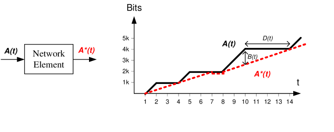
Figure 1: Illustration of $A(t)$, $A^{*}(t)$, $B(t)$ and $D(t)$

In deterministic network calculus, $A(t)$ can be upper-bounded by an arrival curve. That is, for all $0\leq s\leq t$, we have

$$A(s,t)\leq\alpha(t-s),$$

where $\alpha(t)$ is called the arrival curve of $A(t)$.

A busy period is a time period during which the backlog in the network element is always nonzero. For any busy period $(t_{0},t]$, suppose we have

$$A^{*}(t)-A^{*}(t_{0})\geq\beta(t-t_{0}),$$

which means that the network element provides a guaranteed service lower-bounded by $\beta(t-t_{0})$ during the busy period. We can let $t_{0}$ be the beginning of the busy period, that is, the backlog at $t_{0}$ is zero or $A^{*}(t_{0})=A(t_{0})$. Therefore,

$$A^{*}(t)-A(t_{0})\geq\beta(t-t_{0}).$$

The above equation infers $A^{*}(t)\geq\inf_{0\leq s\leq t}{[A(s)+\beta(t-s)]}$, which can be written as

$$A^{*}(t)\geq A\otimes\beta(t),$$ (3)

where $\otimes$ is called the operator of min-plus convolution and $\beta(t)$ is called the service curve of the network element.

II-B Results of Stochastic Network Calculus

We cite the following definitions and theorems from [5][11] except that we define Definition 6 by ourselves.

Definition 1 (virtual-backlog-centric (v.b.c) Stochastic Arrival Curve)

A flow is said to have a virtual-backlog-centric (v.b.c) stochastic arrival curve $\alpha\in{\mathcal{F}}$ with bounding function $f\in\bar{{\mathcal{F}}}$, denoted by $A\sim_{vb}<f,\alpha>$, if for all $t\geq 0$ and all $x\geq 0$, there holds

$$P\{\sup_{0\leq s\leq t}[A(s,t)-\alpha(t-s)]>x\}\leq f(x).$$ (4)

Originally, in deterministic network calculus, we have $A(s,t)\leq\alpha(t-s)$ for all $0\leq s\leq t$. However, there is usually some randomness in stochastic arrival processes and $A(s,t)$ may not be upper-bounded by any arrival curve deterministically (e.g., traffic arrivals in $(s,t]$ can be arbitrarily large in Poisson process). Thus, v.b.c stochastic arrival curve is proposed to tackle this problem. Roughly speaking, $A(s,t)$ can exceed $\alpha(s,t)$ by $x$, but its probability is upper-bounded by $f(x)$ which is a decreasing function of $x$.

Definition 2 (Weak Stochastic Service Curve)

A server $S$ is said to provide a weak stochastic service curve $\beta\in{\mathcal{F}}$ with bounding function $g\in\bar{{\mathcal{F}}}$, denoted by $S\sim_{ws}<g,\beta>$, if for all $t\geq 0$ and all $x\geq 0$, there holds

$$P\{A\otimes\beta(t)-A^{*}(t)>x\}\leq g(x).$$ (5)

In deterministic network calculus, we have $A^{*}(t)\geq A\otimes\beta(t)$, which means that there is a service guarantee denoted by the service curve $\beta(t)$. However, there is usually some randomness in stochastic service process and thus a server may not always provide a guaranteed service curve deterministically. Thus, weak stochastic service curve is proposed to tackle this problem. Roughly speaking, $A^{*}(t)-A\otimes\beta(t)$ can be less than $-x$, but its probability is upper-bounded by $g(x)$ which is a decreasing function of $x$.

The utility of the above definitions is that if we can characterize the traffic by a v.b.c stochastic arrival curve and the server’s service process by a weak stochastic service curve, then we can calculate backlog and delay bounds of the network element by Theorem 1.

Theorem 1 (Backlog and Delay Bounds)

Consider a server fed with a flow $A$. If the server provides a weak stochastic service curve $S\sim_{ws}<g,\beta>$ to the flow and the flow has a v.b.c stochastic arrival curve $A\sim_{vb}<f,\alpha>$, then

(i) The backlog $B(t)$ of the flow in the server at time $t$ satisfies: for all $t\geq 0$ and all $x\geq 0$,

$$P\{B(t)>x\}\leq f\otimes g(x+\inf_{s\geq 0}{[\beta(s)-\alpha(s)]}).$$ (6)

(ii) The delay $D(t)$ of the flow in the server at time $t$ satisfies: for all $t\geq 0$ and all $x\geq 0$,

$$P\{D(t)>x\}\leq f\otimes g(\inf_{s\geq 0}{[\beta(s)-\alpha(s-x)]}).$$ (7)

By definition $\alpha(x)=0$ when $x<0$ in this theorem. Note that as noticed recently by researchers of network calculus, the formula of delay bound in this theorem often returns trivial results, which we will see in Section V.

By now, we have reviewed the key results of stochastic network calculus. Next, we will show how to calculate v.b.c stochastic arrival curve and weak stochastic service curve.

In [11], the author presented a theorem to facilitate calculation of stochastic arrival curves. Before showing the theorem, we first introduce $(\sigma(\theta),\rho(\theta))$-upper constrained [5].

Definition 3 ($(\sigma(\theta),\rho(\theta))$-upper constrained)

A process $A$ is said to be $(\sigma(\theta),\rho(\theta))$-upper constrained (for some $\theta>0$), if for all $0\leq s\leq t$, we have

$$\frac{1}{\theta}\log{\textrm{E}e^{\theta A(s,t)}}\leq\rho(\theta)(t-s)+\sigma(\theta).$$ (8)

This definition is equivalent to $\textrm{E}e^{\theta A(s,t)}\leq e^{\theta\rho(\theta)(t-s)+\theta\sigma(\theta)}$, which means that $A(s,t)$’s moment generating function is upper-bounded. Two related concepts are defined as follows.

Definition 4 ($\theta$-MER / $\theta$-ER)

A process $A$’s minimum envelope rate (MER) with respect to $\theta$ ($\theta$-MER), denoted by $\rho^{*}(\theta)$, is defined as follows:

$$\rho^{*}(\theta)=\lim\sup_{t\rightarrow\infty}\frac{1}{\theta t}\sup_{s\geq 0}\log{\textrm{E}e^{\theta A(s,s+t)}}.$$ (9)

We say that $A$ has an envelope rate (ER) with respect to $\theta$ ($\theta$-ER), denoted by $\rho(\theta)$, if $\rho(\theta)\geq\rho^{*}(\theta)$.

The following theorem expresses the relationship between $\theta$-ER and $(\sigma(\theta),\rho(\theta))$-upper constrained.

Theorem 2 (Relationship of $\theta$-ER and $(\sigma(\theta),\rho(\theta))$-upper constrained)

(i) If $A$ is $(\sigma(\theta),\rho(\theta))$-upper constrained, then $\rho(\theta)$ is $\theta$-ER of $A$.  
(ii) If $A$ has $\theta$-ER $\rho(\theta)<\infty$, then for every $\epsilon>0$ there exists $\sigma_{\epsilon}(\theta)<\infty$ so that $A$ is $(\sigma_{\epsilon}(\theta),\rho(\theta)+\epsilon)$-upper constrained.

Now we have two kinds of traffic characterization: v.b.c stochastic arrival curve and $(\sigma(\theta),\rho(\theta))$-upper constrained. The following theorem establishes the connection between them.

Theorem 3 (v.b.c Stochastic Arrival Curve of $(\sigma(\theta),\rho(\theta))$-upper constrained Process)

Suppose $A(t)$ is $(\sigma(\theta),\rho(\theta))$-upper constrained, then it has a v.b.c stochastic arrival curve $A\sim_{vb}<f,\alpha>$, where

$$\alpha(t) = r\cdot t$$

$$f(x) = \frac{e^{\theta\sigma(\theta)}}{1-e^{\theta(\rho(\theta)-r)}}\cdot e^{-\theta x}$$ (10)

for any $r>\rho(\theta)$ and $x\geq 0$.

This theorem indicates that if we can show that the traffic is $(\sigma(\theta),\rho(\theta))$-upper constrained, then we can get its v.b.c stochastic arrival curve by Eq. (3).

We now introduce the concept of stochastic strict server. This concept was inspired by the observation that a wireless channel can be described by an ideal service process and an impairment process. As we will see in Section III, a wireless node can be modeled as a stochastic strict server.

Definition 5 (Stochastic Strict Server)

A server $S$ is said to be a stochastic strict server providing stochastic strict service curve $\hat{\beta}\in{\mathcal{F}}$ with impairment process $I$ to a flow iff during any backlogged period $(s,t]$, the output $A^{*}(s,t)$ of the flow from the server satisfies

$$A^{*}(s,t)\geq\hat{\beta}(t-s)-I(s,t).$$ (11)

We can easily find the weak stochastic service curve of a stochastic strict server by the following theorem.

Theorem 4 (Weak Stochastic Service Curve of Stochastic Strict Server)

Consider a stochastic strict server $S$ providing a stochastic strict service curve $\hat{\beta}$ with an impairment process $I$. If the impairment process has a v.b.c stochastic arrival curve, or $I\sim_{vb}<g,\gamma>$, and $\beta\in{\mathcal{F}}$, then the server provides a weak stochastic service curve $S\sim_{ws}<g,\beta>$ with

$$\beta(t)=\hat{\beta}(t)-\gamma(t).$$ (12)

So far, we have cited all results of stochastic network calculus which we will use in this paper. Finally, we define stable backlog and stable delay. A natural definition is to check whether the expectation of backlog (or delay) is finite.

Definition 6 (Stable Backlog/Delay)

The backlog $B(t)$ is stable, if

$$\textrm{E}B(t)<\infty,\quad\forall t.$$ (13)

Similarly, the delay $D(t)$ is stable, if

$$\textrm{E}D(t)<\infty,\quad\forall t.$$ (14)

We say that the backlog (or delay) bound of stochastic network calculus is stable if they can derive stable backlog (or delay).

III Stochastic Network Calculus Model of a Wireless Node

In this section we model a wireless node (not restricted to 802.11) by stochastic network calculus. In general, we can define one slot ($t=1$) to be any duration of time and measure traffic amount in any unit (e.g. bits, bytes or packets).

We consider a wireless node. Let $A(t)$ denote the traffic arrived at the node from the application layer. Suppose $A$ is $(\sigma_{A}(\theta_{1}),\rho_{A}(\theta_{1}))$-upper constrained. From Theorem 3, we have $A\sim_{vb}<f,\alpha>$, where

$$\alpha(t) = r_{A}\cdot t$$

$$f(x) = \frac{e^{\theta_{1}\sigma_{A}(\theta_{1})}}{1-e^{\theta_{1}(\rho_{A}(\theta_{1})-r_{A})}}\cdot e^{-\theta_{1}x}$$ (15)

for any $r_{A}>\rho_{A}(\theta_{1})$.

We can model a wireless node by a stochastic strict server. Let the channel capacity be $c$ traffic unit per slot. The departure process $A^{*}(s,t)=\hat{\beta}(s,t)-I(s,t)$ during any backlogged period $(s,t]$, where $\hat{\beta}(t)=c\cdot t$ is the ideal service curve and $I$ is the impairment process due to backoff, channel sharing and transmission errors. Since $I(s,t)\leq c\cdot(t-s)$, $I$ has a finite $\theta$-MER. From Theorem 2, there exist $\sigma_{I}(\theta_{2})$ and $\rho_{I}(\theta_{2})$ so that $I$ is $(\sigma_{I}(\theta_{2}),\rho_{I}(\theta_{2}))$-upper constrained. Based on Theorem 3, we have $I\sim_{vb}<g,\gamma>$, where

$$\gamma(t) = r_{I}\cdot t$$

$$g(x) = \frac{e^{\theta_{2}\sigma_{I}(\theta_{2})}}{1-e^{\theta_{2}(\rho_{I}(\theta_{2})-r_{I})}}\cdot e^{-\theta_{2}x},$$ (16)

for any $r_{I}>\rho_{I}(\theta_{2})$.

From Theorem 4, the node provides a weak stochastic service curve $S\sim_{ws}<g,\beta>$, where

$$\beta(t) = (c-r_{I})\cdot t,$$ (17)

for any $c>r_{I}$.

Furthermore, from Theorem 1, we must have $\alpha(t)\leq\beta(t)$, or equivalently,

$$r_{A}\leq c-r_{I}.$$ (18)

Thus, $P\{B(t)>x\}\leq f\otimes g(x)$. Otherwise, if $\alpha(t)>\beta(t)$, we get a trivial backlog bound, $P\{B(t)>x\}\leq f\otimes g(-\infty)=\infty$.

IV Stability Condition of a Wireless Node

One fundamental question we need to address is under what condition we can get stable $B(t)$ and $D(t)$ from stochastic network calculus, i.e., $\textrm{E}B(t)<\infty$ and $\textrm{E}D(t)<\infty$. Before presenting our result, we first define the concept of envelop average rate.

Definition 7 (Envelop Average Rate)

The envelop average rate of a process $A$, denoted by $a_{A}$, is defined as

$$a_{A}=\lim_{t\rightarrow\infty}\sup_{s\geq 0}\frac{\textrm{E}A(s,s+t)}{t}.$$ (19)

Let $a_{A}$ and $a_{I}$ be the envelop average rate of $A$ and $I$, respectively. The following proposition shows the stability condition.

Proposition 1 (Stability Condition)

A wireless node has stable backlog and stable delay if

$$a_{A}<c-a_{I}.$$ (20)

Proof: We have shown that $P\{B(t)>x\}\leq f\otimes g(x)$ if Eq. (18) holds. Thus, for any $t$,

$$\textrm{E}B(t) = \sum_{i=0}^{\infty}P\{B(t)=i+1\}\cdot(i+1)$$ (21)

$$< \sum_{i=0}^{\infty}P\{B(t)>i\}\cdot(i+1)$$

$$\leq \sum_{i=0}^{\infty}f\otimes g(i)\cdot(i+1)<\infty.$$

Since $f(x)$ and $g(x)$ are exponentially decreasing functions according to Eq. (III) and Eq. (III), $f\otimes g(x)$ is an exponentially decreasing function. Thus we have, for any $t$, $\textrm{E}B(t)<\infty$. It is easy to see that for any $t$, $\textrm{E}D(t)<\infty$. Otherwise, the service time is $\infty$ and thus $\lim_{t\rightarrow\infty}\textrm{E}B(t)=\infty$ which contradicts Eq. (21).

Now we examine Eq. (18). From Eq. (III) and Eq. (III), $r_{A}=\rho_{A}(\theta_{1})+\epsilon$ and $r_{I}=\rho_{I}(\theta_{2})+\epsilon$ for any $\epsilon>0$. Thus, Eq. (18) is equivalent to

$$\rho_{A}(\theta_{1})\leq c-\rho_{I}(\theta_{2})-2\epsilon.$$

From Theorem 2, we have $\rho_{A}(\theta_{1})=\rho_{A}^{*}(\theta_{1})+\epsilon_{1}$ and $\rho_{I}(\theta_{2})=\rho_{I}^{*}(\theta_{2})+\epsilon_{1}$ for any $\epsilon_{1}>0$, where $\rho_{A}^{*}(\theta_{1})$ and $\rho_{I}^{*}(\theta_{2})$ are $\theta$-MERs of $A$ and $I$, respectively. Equivalently, we have

$$\rho_{A}^{*}(\theta_{1})\leq c-\rho_{I}^{*}(\theta_{2})-2(\epsilon+\epsilon_{1}).$$ (22)

Using Taylor expansion on $\rho_{A}^{*}(\theta_{1})$, we have

$$\rho_{A}^{*}(\theta_{1}) = \lim\sup_{t\rightarrow\infty}\frac{1}{\theta_{1}t}\sup_{s\geq 0}\log{\textrm{E}e^{\theta_{1}A(s,s+t)}}$$

$$= \lim{\sup_{t\rightarrow\infty}{\frac{1}{\theta_{1}t}\sup_{s\geq 0}{\log{\textrm{E}(1+\theta_{1}A(s,s+t)+O(\theta_{1}^{2}))}}}}$$

$$= \lim{\sup_{t\rightarrow\infty}{\frac{1}{\theta_{1}t}\sup_{s\geq 0}{\log{(1+\theta_{1}\textrm{E}A(s,s+t)+O(\theta_{1}^{2}))}}}}$$

$$= \lim{\sup_{t\rightarrow\infty}{\frac{1}{\theta_{1}t}\sup_{s\geq 0}{[\theta_{1}\textrm{E}A(s,s+t)+O(\theta_{1}^{2})]}}}.$$

Therefore,

$$\lim_{\theta_{1}\rightarrow 0}\rho_{A}^{*}(\theta_{1})=\lim_{t\rightarrow\infty}\sup_{s\geq 0}{\frac{\textrm{E}A(s,s+t)}{t}}=a_{A}.$$

Similarly,

$$\lim_{\theta_{2}\rightarrow 0}\rho_{I}^{*}(\theta_{2})=a_{I}.$$

Therefore, there exist $\theta_{1}$ and $\theta_{2}$ so that $\rho_{A}^{*}(\theta_{1})\leq a_{A}+\epsilon_{2}$ and $\rho_{I}^{*}(\theta_{2})\leq a_{I}+\epsilon_{2}$ for any enough small $\epsilon_{2}>0$. So Eq. (22) is satisfied if

$$a_{A}\leq c-a_{I}-2(\epsilon+\epsilon_{1}+\epsilon_{2}).$$

Since $\epsilon$, $\epsilon_{1}$ and $\epsilon_{2}$ can be arbitrarily small, the above equation is satisfied when

$$a_{A}<c-a_{I}.$$

 
Remarks: Since the proof is based on theorems of stochastic network calculus, it indicates that we can get stable backlog and delay bounds by stochastic network calculus as long as the condition of Eq. (20) holds. Since this condition is very general, we conclude that theoretically stochastic network calculus is effective.

V 802.11 Backlog and Delay Bounds

In this section, we apply the results in the previous section to calculate backlog and delay bounds for an 802.11 WLAN node. For simplicity, we assume there are $n$ identical stations (or nodes) sending packets to an access point. All nodes operate in Distributed Coordination Function (DCF) mode with RTS/CTS turned off[17]. We consider an ideal channel, that is, transmission errors are only caused by collisions. Two packets are collided if their transmissions overlap in time. Besides, we assume that all DATA packets are of the same size.

V-A 802.11 DCF

A node with a DATA packet (or simply packet) to transmit first monitors the channel activity. If the channel is idle for a period of time equal to a distributed interframe space (DIFS), the node transmits. Otherwise, if the channel is sensed busy (either immediately or during the DIFS), the node backs off, in which the node defers channel access by a random number of idle slots within a contention window ($CW$), ranging from 0 to $CW-1$. When the backoff counter reaches zero and expires, the node can access the channel. During the backoff period, if the node detects a busy channel, it freezes the backoff counter and the backoff process is resumed once the channel is idle for a duration of DIFS. To avoid channel capture, a node must wait a random backoff time between two consecutive new packet transmissions, even if the channel is sensed idle for a duration of DIFS. Once the packet is received successfully, the receiver will return an ACK after a short interframe space (SIFS). Note that SIFS is shorter than an idle slot so that there is no collision caused by a DATA packet and an ACK.

802.11 uses the truncated exponential backoff technique to set its $CW$. For example, in 802.11b, the initial $CW$ is $CW_{min}=32$. Each time a collision occurs, $CW$ doubles its size, up to a maximum of $CW_{max}=1024$. When the packet is successfully transmitted, $CW$ is reset to $CW_{min}$. The packet is dropped when it is retransmitted for six times and still not transmitted successfully. Fig. 2 shows some parameters of 802.11b used in our paper.

Basic rate	1 Mbps
Data rate	11 Mbps
PHY header	24 bytes
ACK header	14 bytes
MAC header	28 bytes
SIFS	10 $\mu$s
DIFS	50 $\mu$s
Idle slot	20 $\mu$s
$CW_{min}$	32
$CW_{max}$	1024
Retransmission limit	6

Figure 2: 802.11b parameters

The duration of an ACK is the duration of a PHY header and an ACK header transmitted at basic rate, i.e., $\frac{(24+14)\cdot 8}{10^{6}}=304\mu$s. The duration of a DATA packet is the duration of an PHY header transmitted at basic rate plus the duration of an MAC header and its upper-layer payload transmitted at data rate. For example, suppose the upper-layer payload is $256$ bytes, then the duration of the DATA packet is $\frac{24\cdot 8}{10^{6}}+\frac{(28+256)\cdot 8}{11\cdot 10^{6}}=398.5\mu$s.

V-B Service Curve

Since we only consider packets of equal size, we can measure traffic amount in packets. For simplicity, we measure time duration (e.g. SIFS, DIFS, DATA and ACK) in idle slots and we define that one slot in network calculus ($t=1$) is equal to $L$ idle slots, where

$$L=DIFS+DATA+SIFS+ACK.$$ (23)

Note that sometimes ”idle slot” only refers to a time period and it may not be idle. To avoid confusion in the following context, we will use ”idle slot” (italic) to denote that the ”idle slot” is indeed idle.

In practice, it is difficult to calculate the impairment process $I$ accurately since $I$ depends on the complex interactions of traffic arrival and DCF. In this section, we perform the worst case analysis based on an existing model of 802.11[18].

We assume that the system is in saturated condition, that is, the backlog at each node is always nonzero. Let $\tau$ denote the transmission attempt probability per idle slot by a node and let $\gamma$ denote the conditional collision probability given that there is a transmission. We assume $\gamma$ is constant and independent for each transmission. Intuitively, this assumption becomes more accurate when the number of nodes $n$ increases. In [18], the authors derived a general formula relating $\tau$ to $\gamma$, which is

$$\tau=\frac{1+\gamma+\gamma^{2}+...+\gamma^{6}}{b_{0}+\gamma b_{1}+\gamma^{2}b_{2}+...+\gamma^{6}b_{6}}.$$ (24)

This equation can be explained as follows. The numerator is the expected number of transmission attempts of a packet. The denominator is the expected total backoff duration (in idle slots) of a packet, where $b_{i}$ is the mean backoff duration plus 1 (the 1 refers to the first idle slot of packet transmission) after the $i$th collision. In 802.11, $b_{i}=\frac{2^{i}\cdot CW_{min}}{2}$ where $0\leq i\leq 6$. A packet suffering six collisions will be dropped from its buffer. In our model, we do not consider packet drops, which yields upper bounds of backlog and delay.

The independence assumption of $\gamma$ implies that each transmission ”sees” the system at steady state. Therefore, each node transmits with the same probability $\tau$. This yields

$$\gamma=1-(1-\tau)^{n-1}.$$ (25)

Combining Eq. (24) and Eq. (25), we can solve $\tau$ and $\gamma$.

We introduce the following notations for an 802.11 node. The probability of no transmissions at an idle slot, denoted by $P_{nt}$, is $(1-\tau)^{n}$. The probability of having at least one transmission at an idle slot, denoted by $P_{t}$, is $1-P_{nt}$. The probability of a given node starting a successful transmission at an idle slot, denoted by $P_{s}$, is $\tau(1-\gamma)$. For the given node, the probability of the other nodes starting transmissions at an idle slot, denoted by $P_{o}$, is $P_{t}-P_{s}=\gamma$.

Fig. 3 plots Eq. (24) in dashed line and Eq. (25) in solid line when $n=10$, $20$ and $100$. The points of intersection are the solution of $\gamma$ and $\tau$ for different $n$. When $n$ increases, $\gamma$ increases and $\tau$ decreases. Consequently, $P_{nt}$ and $P_{o}$ increases, but $P_{s}$ decreases. Therefore, the assumption of saturated condition gives the worst-case analysis.

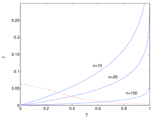
Figure 3: The Plots of Eq. (24) and Eq. (25)

An 802.11 node can be seen as a stochastic strict server. Clearly, the stochastic strict service curve $\hat{\beta}(t)=t$, which means that one packet is transmitted during one slot in the ideal case. In order to characterize the impairment process $I$, it is crucial to know $\textrm{E}e^{\theta I(s,s+t)}$ which we calculate as follows.

We consider the transmissions of a given 802.11 node during $t$ slots. From Eq. (23), there are $tL$ idle slots in $t$ slots, indexed $1$, $2$, …, $tL$. At the first or the last idle slot, the transmission (if any) can be incomplete, that is, the transmission can start before the first idle slot or it can end after the last idle slot. We assume that at the first slot there is always a complete transmission by any of the other nodes except the given node, which actually overestimates $\textrm{E}e^{\theta I(s,s+t)}$. Suppose there are $i$ complete transmissions and zero or one incomplete transmission within the remaining $(t-1)L$ idle slots. The incomplete transmission occupies the last $k$ idle slots where $0\leq k\leq L-1$ ($k=0$ means that the last transmission is actually complete). Thus, there are $(t-i-1)L-k$ idle slots of no transmissions within the $t$ slots. The probability of $i$ complete transmissions and the last $k$ idle slots occupied by an incomplete transmission, denoted by $p_{k,i}$, is $C_{(t-i-1)L-k+i}^{i}P_{nt}^{(t-i-1)L-k}P_{t}^{i}$. Furthermore, the probability of the given node having $j$ successful complete transmissions on condition that there are $i$ complete transmissions, denoted by $p_{i,j}$, is $C_{i}^{j}(P_{s}/P_{t})^{j}(P_{o}/P_{t})^{i-j}$. Finally, we have $\textrm{E}e^{\theta I(s,s+t)}$ is upper-bounded by

$$P_{t}\cdot\sum_{k=1}^{L-1}\sum_{i=0}^{t-2}\sum_{j=0}^{i}p_{k,i}p_{i,j}e^{\theta(t-j)}+\sum_{i=0}^{t-1}\sum_{j=0}^{i}p_{0,i}p_{i,j}e^{\theta(t-j)}.$$ (26)

The first term is for the case that the last transmission is incomplete and the second term is for the case that the last transmission is complete.

In general, we do not have an analytical form of Eq. (26), so we resort to numerical methods and use Algorithm 1 to obtain $\sigma_{I}(\theta)$ and $\rho_{I}(\theta)$ (see Appendix A-1). This algorithm is immediately inspired from Definition 3. Then we can use Eq. (III) and (17) to obtain the node’s weak stochastic service curve.

Scenario 1:

10 identical nodes sending packets to one access point

The payload of a DATA packet is $256$ bytes

Figure 4: Parameters of Scenario 1

We illustrate the above calculations in Scenario 1 (see Fig. 4). From Eq. (24) and (25), $\tau=0.037$ and $\gamma=0.293$. Thus, $P_{nt}=0.680$, $P_{t}=0.320$, $P_{s}=0.027$ and $P_{o}=0.293$. Let $M(t)$ be the value of Eq. (26). Fig. 5 shows $M(t)$ and its $\sigma(\theta),(\rho(\theta))$-upper constrained curve when $\theta=1$. We have $\rho(1)=0.948$ and $\sigma(1)=0.096$, as calculated by Algorithm 1.

Figure 5: Scenario 1: the $(\sigma(1),\rho(1))$-upper constrained curve of a node’s $M(t)$

Furthermore, from Eq. (III) and (17) we have $S\sim_{ws}<g,\beta>$ where

$$\beta(t) = (1-r_{I})\cdot t$$

$$g(x) = \frac{e^{0.096}}{1-e^{0.948-r_{I}}}\cdot e^{-x},$$

for any $1>r_{I}>0.948$. Fig. 6 plots $\beta(t)$ and $g(t)$ when $r_{I}=0.968$.

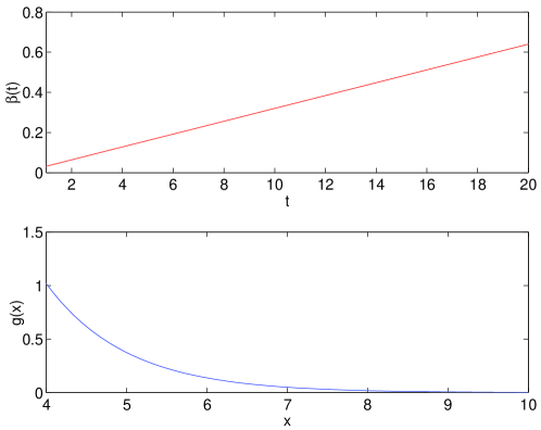
Figure 6: Scenario 1: a node’s Weak stochastic service curve

V-C Stability Condition

Before calculating the bounds, we first derive the stability condition. Since $\hat{\beta}(t)=t$, the channel capacity $c=1$ packet per slot. Because $1-a_{I}$ is actually the percentage of the node’s successful transmission time, by Proposition 1, the stability condition of 802.11 is

$$a_{A}<1-a_{I}=\frac{P_{s}\cdot L}{P_{nt}+P_{t}\cdot L}.$$ (27)

V-D Backlog and Delay Bounds

We can immediately calculate backlog bounds by applying Eq. (III)-(17) into Theorem 1. The only technical issue is to select proper $\theta_{1}$ and $\theta_{2}$ a obtain tight bounds. Clearly, $f(x)$ depends on $\theta_{1}$ and $r_{A}$, and $g(x)$ depends on $\theta_{2}$ and $r_{I}$. According to Eq. (18), we have $r_{A}\leq 1-r_{I}$ and $P\{B(t)>x\}\leq f\otimes g(x)$. In addition, $r_{A}$ ($r_{I}$) should be set as large as possible because $f(x)$ ($g(x)$) decreases with $r_{A}$ ($r_{I}$). Considering the above conditions, we have

$$P\{B(t)>x\}\leq\min[f\otimes g(x)]$$

subject to

$$r_{A}>\rho_{A}(\theta_{1}),r_{I}>\rho_{I}(\theta_{2})\ \textnormal{and}\ r_{A}+r_{I}=1.$$ (28)

In general, we do not have an analytical solution of $\min[f\otimes g(x)]$ and we resort to numerical methods and use Algorithm 2 to get a near-optimal solution (see Appendix A-2).

As noticed recently by researchers of network calculus, the delay bound in Theorem 1 often returns trivial results. In our model in Section III, it is easy to see that $P\{D(t)>x\}\leq f\otimes g(0)=1$. We propose the following way to estimate delay bound. Little’s law states that the average number of customers in a queueing system is equal to the average arrival rate of customers to that system, times the average time spent in that system[1]. Let the average arrival rate is $\lambda$. Assume the system can reach steady state when $t\rightarrow\infty$. Then we have the average backlog is $\lim_{t\rightarrow\infty}\textrm{E}B(t)$ and the average delay of each packet is greater than or equal to $\lim_{t\rightarrow\infty}\textrm{E}D(t)$ (by its definition in Eq. (2), $D(t)$ can be less than the delay of the bottom-of-line packet at $t$). Therefore, by Little’s law, we have

$$\lim_{t\rightarrow\infty}\textrm{E}D(t)\leq\frac{\lim_{t\rightarrow\infty}\textrm{E}B(t)}{\lambda}.$$ (29)

Finally, we apply Markov’s inequality to the above equation and we have

$$P\{\lim_{t\rightarrow\infty}D(t)\geq x\}\leq\frac{\lim_{t\rightarrow\infty}\textrm{E}B(t)}{\lambda x}.$$ (30)

Besides, according to Eq. (21), $\textrm{E}B(t)\leq\sum_{i=0}^{\infty}{P\{B(t)>i\}\cdot(i+1)}$. And we can use Eq. (V-D) to bound $P\{B(t)>i\}$. Note that Eq. (30) is derived when $t\rightarrow\infty$. In practice, we can use this result to estimate delay bound when $t$ is sufficiently large.

VI Performance Evaluation

In this section, we use ns-2 simulations to verify our derived backlog and delay bounds for Poisson and constant bit rate (CBR) traffic arrivals. We carry out all experiments for Scenario 1 (Fig. 4). Each simulation duration is 100 seconds (s) which is long enough to let a node transmit thousands of packets. Each data point (e.g. $P\{B(t)>x\}$) is calculated over 100 independent simulations.

VI-A Poisson Traffic

Let $\lambda$ be the average traffic rate (packets/slot). In this case, we have $a_{A}=\lambda$ (see Definition 7). For Poisson traffic, we have

$$Ee^{\theta A(s,s+t)}=\sum_{i=0}^{\infty}\frac{(\lambda t)^{i}}{i!}e^{-\lambda t}e^{\theta i}=e^{\lambda t(e^{\theta}-1)},$$ (31)

where $\frac{(\lambda t)^{i}}{i!}e^{-\lambda t}$ is the probability of $i$ packets arriving within $(s,s+t]$. From the above equation, Poisson traffic is $(0,\frac{\lambda(e^{\theta}-1)}{\theta})$-upper constrained and we can obtain its arrival curve by Eq. (III).

From Eq. (27), backlogs are stable when $\lambda<0.079$ (packet per slot). In Fig. 7, we plot the average backlog $\textrm{E}[B(t)]$ at $t=50s$ and $\lambda=0.077$, $0.079$ and $0.081$ in ns-2 simulations. We observe that there is sudden jump when $\lambda=0.081$, indicating the critical point of stability is indeed around $0.079$. This figure also indicates the accuracy of the 802.11 model in Eq. (24) and Eq. (25).

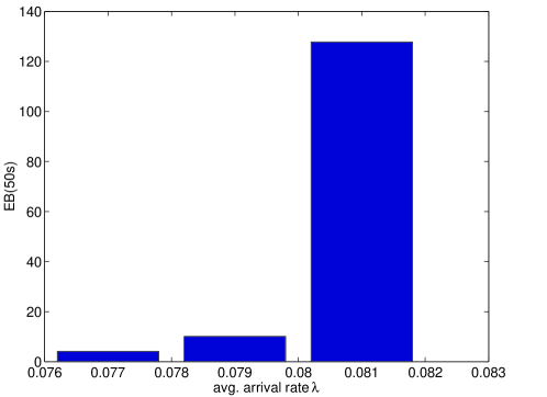
Figure 7: $\textrm{E}B(t)$ ($t=50$s) when $\lambda=0.077,0.079,0.081$

Experiment 1(Scenario 1 with low Poisson traffic load) We set $\lambda=0.04$ to simulate low traffic load.

Fig. 8(a) shows $P\{B(t)>x\}$ in ns-2 simulations and Fig. 8(b) shows the upper bound of $P\{B(t)>x\}$ calculated by Eq. (V-D). Note that stochastic network calculus gives very loose upper bounds. There may be two reasons. One is that we use the worst-case analysis in deriving the weak stochastic service curve of 802.11. The other is that there are many relaxations in proving the theorems of stochastic network calculus[11]. For example, relaxations are used in deriving $f(x)$ in Theorem 3 [12], and this theorem is popularly used in deriving arrival curves and service curves (see Section III). The first reason may not be the key reason because we will see in Experiment 2 the bound is even looser when we increase arrival rate and make the channel near saturated. The second reason seems to be the key reason. We will see in Experiment 3 that backlog bounds improve substantially for CBR traffic where we are able to derive the arrival curve by hand without using Theorem 3. This indicates that refinements are needed in stochastic network calculus so as to tighten the bounds. Moreover, we found that backlog bounds are sensitive to adjusting parameters (i.e., $\theta_{1}$, $\theta_{2}$, $r_{A}$ and $r_{I}$). So it is necessary to use Algorithm 2 to minimize the bounds.

We also conduct simulations to verify delay bounds at $t=50s$. Since the backlog bounds are too loose, in order to avoid trivial validation, we use $\textrm{E}B(t)$ in ns-2 simulations to validate Eq. (29) and Eq. (30) (assume that $t=50$s is sufficiently large so that we can apply these equations). Actually, we get $\textrm{E}D(t)\leq 0.0205s$ by Eq. (29), which tightly bounds $\textrm{E}D(t)=0.0186s$ in ns-2 simulations. Fig. 8(c) shows $P\{D(t)\geq x\}$ in ns-2 simulations and Fig. 8(d) shows the upper bound of $P\{D(t)\geq x\}$ calculated by Eq. (30). Clearly, $P\{D(t)\geq x\}$ is upper-bounded by Eq. (30).

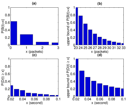
Figure 8: Experiment 1: When $t=50s$ (a) $P\{B(t)>x\}$ (b) upper bound of $P\{B(t)>x\}$ (c) $P\{D(t)\geq x\}$ (d) upper bound of $P\{D(t)\geq x\}$

Experiment 2(Scenario 1 with high Poisson traffic load) We set $\lambda=0.07$ to simulate high traffic load.

Fig. 9(a) shows $P\{B(t)>x\}$ in ns-2 simulations and Fig. 9(b) shows the upper bound of $P\{B(t)>x\}$ calculated by Eq. (V-D). In this case, $\theta_{1}$ ($\theta_{2}$) is much smaller than that of Experiment 1 so as to satisfy the constraint in Eq. (V-D), resulting in looser $f(x)$ and $g(x)$. Therefore, stochastic network calculus gives further loose backlog bounds.

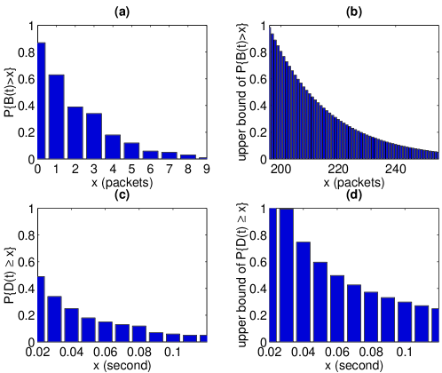
Figure 9: Experiment 2: When $t=50s$ (a) $P\{B(t)>x\}$ (b) upper bound of $P\{B(t)>x\}$ (c) $P\{D(t)\geq x\}$ (d) upper bound of $P\{D(t)\geq x\}$

We also conduct simulations to verify delay bounds at $t=50s$. Since the backlog bounds are too loose, in order to avoid trivial validation, we use $\textrm{E}B(t)$ in ns-2 simulations to validate Eq. (29) and Eq. (30) (assume that $t=50$s is sufficiently large so that we can apply these equations). Actually, we get $\textrm{E}D(t)\leq 0.0299s$ by Eq. (29), which tightly bounds $\textrm{E}D(t)=0.0296s$ in ns-2 simulations. Fig. 9(c) shows $P\{D(t)\geq x\}$ in ns-2 simulations and Fig. 9(d) shows the upper bound of $P\{D(t)\geq x\}$ calculated by Eq. (30). Clearly, $P\{D(t)\geq x\}$ is upper-bounded by Eq. (30).

VI-B CBR Traffic

Let $\lambda$ be the average traffic rate (packets/slot). In this case, we have $a_{A}=\lambda$. It is easy to see that $\sup_{0\leq s\leq t}[A(s,t)-\lambda\cdot(t-s)]<1$ for all $t$ because packets arrive one by one in a constant time interval. Thus, we have $A\sim_{vb}<f,\alpha>$ where

$$\alpha(t) = \lambda t$$

$$f(x) = \left\{\begin{array}[]{ll}0,&\ x\geq 1\\ 1,&\ x<1\end{array}\right.$$ (34)

Again, from Eq. (27), the stability condition is $\lambda<0.079$ (packet per slot). In Fig. 10, we plot the average backlog $\textrm{E}[B(t)]$ at $t=50s$ for $\lambda=0.077$, $0.079$ and $0.081$ in ns-2 simulations. We observe that there is sudden jump when $\lambda=0.081$, indicating the critical point of stability is indeed around $0.079$. This figure also indicates the accuracy of the 802.11 model in Eq. (24)and(25).

Figure 10: $\textrm{E}B(t)$ ($t=50$s) when $\lambda=0.077,0.079,0.081$

Experiment 3(Scenario 1 with low CBR traffic load) We set $\lambda=0.04$ to simulate low traffic load.

Fig. 11(a) shows $P\{B(t)>x\}$ in ns-2 simulations and Fig. 11(b) shows upper bound of $P\{B(t)>x\}$ calculated by Eq. (V-D). The backlog bounds are much tighter in CBR traffic than those in Poisson traffic (see Experiment 1). The main reason is that we can derive a tight $f(x)$ by hand instead of by Theorem 3.

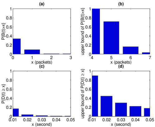
Figure 11: Experiment 3: When $t=50s$ (a) $P\{B(t)>x\}$ (b) upper bound of $P\{B(t)>x\}$ (c) $P\{D(t)\geq x\}$ (d) upper bound of $P\{D(t)\geq x\}$

We also conduct simulations to verify delay bounds at $t=50s$. Since the backlog bounds are still loose, in order to avoid trivial validation, we use $\textrm{E}B(t)$ in ns-2 simulations to validate Eq. (29) and Eq. (30) (assume that $t=50$s is sufficiently large so that we can apply these equations). Actually, we get $\textrm{E}D(t)\leq 0.0090s$ by Eq. (29), which tightly bounds $\textrm{E}D(t)=0.0089s$ in ns-2 simulations. Fig. 11(c) shows $P\{D(t)\geq x\}$ in ns-2 simulations and Fig. 11(d) shows the upper bound of $P\{D(t)\geq x\}$ calculated by Eq. (30). Clearly, $P\{D(t)\geq x\}$ is upper-bounded by Eq. (30).

Experiment 4(Scenario 1 with high CBR traffic load) We set $\lambda=0.07$ to simulate high traffic load.

Fig. 12(a) shows $P\{B(t)>x\}$ in ns-2 simulations and Fig. 12(b) shows the upper bound of $P\{B(t)>x\}$ calculated by Eq. (V-D). The backlog bounds are much tighter in CBR traffic than those in Poisson traffic (see Experiment 2) because $f(x)$ is tight here.

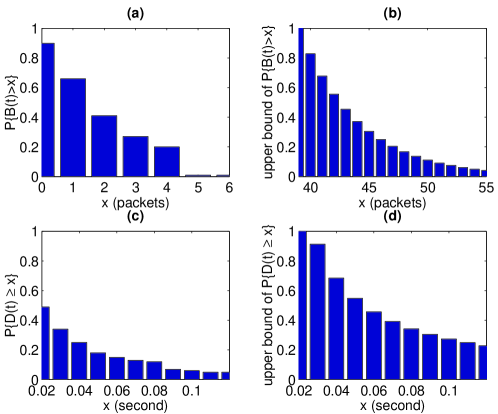
Figure 12: Experiment 4: When $t=50s$ (a) $P\{B(t)>x\}$ (b) upper bound of $P\{B(t)>x\}$ (c) $P\{D(t)\geq x\}$ (d) upper bound of $P\{D(t)\geq x\}$

We also conduct simulations to verify delay bounds at $t=50s$. Since the backlog bounds are still loose, in order to avoid trivial validation, we use $\textrm{E}B(t)$ in ns-2 simulations to validate Eq. (29) and Eq. (30) (assume that $t=50$s is sufficiently large so that we can apply these equations). Actually, we get $\textrm{E}D(t)\leq 0.0274s$ by Eq. (29), which is close to (although does not bound) $\textrm{E}D(t)=0.0296s$ in ns-2 simulations. Fig. 12(c) shows $P\{D(t)\geq x\}$ in ns-2 simulations and Fig. 12(d) shows the upper bound of $P\{D(t)\geq x\}$ calculated by Eq. (30). Clearly, $P\{D(t)\geq x\}$ is upper-bounded by Eq. (30).

To sum up, the current version of stochastic network calculus often derives loose bounds when compared with simulations, especially in the case of high traffic load. Therefore, stochastic network calculus may not be effective in practice.

VII Related Work

In this section, we first present relate work on stochastic network calculus and then on the performance analysis of 802.11.

The increasing demand on transmitting multimedia and other real time applications over the Internet has motivated the study of quality of service guarantees. Towards it, stochastic network calculus, the probabilistic version of the deterministic network calculus [2][3][4][5], has been recognized by researchers as a promising step. During its development, traffic-amount-centric (t.a.c) stochastic arrival curve is proposed in [6], virtual-backlog-centric (v.b.c) stochastic arrival curve is proposed in [9] and maximum-backlog-centric (m.b.c) stochastic arrival curve is proposed in [11]. Weak stochastic service curve is proposed in [7][8] and stochastic service curve is proposed in [10]. In [11], Jiang showed that only the combination of m.b.c stochastic arrival curve and stochastic service curve has all five basic properties required by a network calculus (i.e., superposition, concatenation, output characterization, per-flow service, service guarantees) and the other combinations only have parts of these properties. Jiang also proposed the concept of stochastic strict server to facilitate calculation of stochastic service curve. Moreover, he presented independent case analysis to obtain tighter performance bounds for the case that flows and servers are independent. However, there are a few bugs in his results recently found by researchers of network calculus, such as the trivial delay bound in Theorem 3.5[11] and Theorem 5.1. Therefore, we adopt v.b.c stochastic arrival curve and weak stochastic service curve in our study since we only consider backlog and delay bounds (i.e., service guarantee), ignoring the other properties.

There have been some applications of stochastic network calculus. In [13], Jiang et al. analyzed a dynamic priority measurement-based admission control (MBAC) scheme based on stochastic network calculus. In [14], Liu et al. applied stochastic network calculus to studying the conformance deterioration problem in networks with service level agreements. In [15], based on stochastic network calculus, X. Yu et al. developed several upper bounds on the queue length distribution of Generalized Processor Sharing (GPS) scheduling discipline with long range dependent (LRD) traffic. They also extended the GPS results to a packet-based GPS (PGPS) system. Finally, Agharebparast et al. modeled the behavior of a single wireless link using stochastic network calculus [16]. However, little effort has been made on applying stochastic network calculus to multi-access communication systems such as 802.11.

Existing work on the performance of 802.11 has focused primarily on its throughput and capacity. In [19], Bianchi proposed a Markov chain throughput model of 802.11. In [18], Kumar et al. proposed a probability throughput model which is simpler than Bianchi’s model. In our paper, we adopt Kumar’s model to derive the service curve of 802.11. There are also some work on queueing analysis of 802.11. In [20], Zhai et al. assumed Poisson traffic arrival and proposed an M/G/1 queueing model of 802.11. More generally, Tickoo proposed a G/G/1 queueing model of 802.11[21][22]. To our best knowledge, we are the first to model the queueing process of 802.11 based on stochastic network calculus.

VIII Conclusion and Future Work

In this paper, we presented a stochastic network calculus model of 802.11. From stochastic network calculus, we first derived the general stability condition of a wireless node. Then we derived the stochastic service curve and the specific stability condition of an 802.11 node based on an existing model of 802.11. Thus, we obtained the backlog and delay bounds of the node by using the corresponding theorem of stochastic network calculus. Finally, we carried out ns-2 simulations to verify these bounds.

There are some open problems for future work. First, we derived the service curve based on an existing 802.11 model. Thus, the accuracy of the service curve depends on the accuracy of the model. An open question may be whether we can derive the service curve of 802.11 without using any existing models. Second, we assumed the worst-case condition (i.e., saturate condition) in our analysis. Can we remove this conservative assumption? Besides, under the worst-case assumption, we can assume flows and servers are independent and perform independent case analysis obtaining tighter backlog and delay bounds. This is also one of our future work. Third, we observe that the derived bounds are loose when compared with ns-2 simulations, calling for further improvements in the current version of stochastic network calculus.

Appendix A-1: Algorithm 1 (Numerical Calculation of $\sigma_{I}(\theta)$ and $\rho_{I}(\theta)$)

1. Let $M(t)=\sup_{s\geq 0}\{\frac{1}{\theta}\log{\textrm{E}e^{\theta I(s,s+t)}}\}$. Obviously, $M(t)$ is an increasing function of $t$ with $M(0)=0$. We define axes $t$ and axes $t_{\bot}$ (vertical to $t$) on a plane, and plot $M(t)$ on it. We define the slope of $M(t)$, $s(t)=M(t)-M(t-1)$.

2. We calculate $s(t)$ for $t=1,2,3,...$ until it converges at some $t^{*}$, i.e., $(1-\epsilon)\cdot s(t^{*}-1)\leq s(t^{*})\leq(1+\epsilon)\cdot s(t^{*}-1)$ where $\epsilon$ is a small number, e.g. $10^{-5}$.

3. We draw a straight line $l(t)$ with the slope $s(t^{*})$ crossing the point $\big{(}t^{*},M(t^{*})\big{)}$. Obviously, the line crosses the point $\big{(}0,M(t^{*})-s(t^{*})t^{*}\big{)}$. The maximum displacement between $M(t)$ and $l(t)$ (in the direction of $t_{\bot}$), $v_{m}=\max_{0\leq t\leq t^{*}}\{M(t)-l(t)\}$. We shift $l(t)$ by $v_{m}$ in the direction of $t_{\bot}$ and get $\tilde{l}(t)$. Clearly, $\tilde{l}(t)$ upperbounds $M(t)$. In other words, we have $\rho_{I}(\theta)=s(t^{*})$ and $\sigma_{I}(\theta)=M(t^{*})-s(t^{*})t^{*}+v_{m}$.

Appendix A-2: Algorithm 2 (Numerical Calculation of Eq. (V-D))

In each iteration, we generate a sample of $\theta_{1}$, $\theta_{2}$, $r_{A}$ and $r_{I}$. If they satisfy the condition of Eq. (V-D), we calculate $\min[f\otimes g(x)]$ for the current and past iterations until it converges. Sample generations can use the interpolation or Monte Carlo method over valid ranges of the variables.

References

- [1] L. Kleinrock, ”Queueing Systems. Volume 1: Theory,” Wiley Interscience, 1975.
- [2] R. L. Cruz, ”A Calculus for Network Delay, Part I: Network Elements in Isolation,” IEEE Trans. Information Theory, 37(1), pp. 114C131, 1991.
- [3] R. L. Cruz, ”A Calculus for Network Delay, Part II: Network Analysis,” IEEE Trans. Information Theory, 37(1), pp. 132C141, 1991.
- [4] J.-Y. Le Boudec and P. Thiran, ”Network Calculus: A Theory of Deterministic Queueing Systems for the Internet,” Springer-Verlag, 2001.
- [5] C.-S. Chang, ”Performance Guarantees in Communication Networks,” Springer-Verlag, 2000.
- [6] C. Li, A. Burchard, and J. Liebeherr, ”A Network Calculus with Effective Bandwidth,” Technical Report, CS-2003-20, University of Virginia, 2003.
- [7] R. L. Cruz, ”Quality of Service Management in Integrated Services Networks,” Procs., 1st CWC Semi-Annual Research Review, UCSD, 1996.
- [8] Y. Liu, C.-K. Tham, and Y. Jiang, ”A stochastic Network Calculus,” Technical report, ECE-CCN-0301, National University of Singapore, 2004.
- [9] Y. Jiang and P. J. Emstad, ”Analysis of Stochastic Service Guarantees in Communication Networks: A Traffic Model,” Procs., International Teletraffic Congress, 2005.
- [10] Y. Jiang and P. J. Emstad, ”Analysis of Stochastic Service Guarantees in Communication Networks: A Server Model,” Procs., IEEE IWQoS, 2005.
- [11] Y. Jiang, ”A Basic Stochastic Network Calculus,” Procs., SIGCOMM, pp. 123-134, 2006.
- [12] Y. Jiang and Y. Liu, ”Stochastic Network Calculus,” Springer, 2008.
- [13] Y. Jiang, P. Emstad, A. Nevin, V. Nicola, and M. Fidler, ”Measurement-Based Admission Control for a Flow-Aware Network,” Procs., EuroNGI 1st Conference on Next Generation Internet Networks - Traffic Engineering, 2005.
- [14] Y. Liu, C.-K. Tham, and Y. Jiang, ”Comformance Analysis in Networks with Service Level Agreements,” Computer Networks, vol. 47, pp. 885-906, 2005.
- [15] X. Yu, I. L.-J. Thng, Y. Jiang, and C. Qiao, ”Queueing Processes in GPS and PGPS with LRD Traffic Inputs,” IEEE/ACM Trans. Networking, 13(3):676-689, 2005.
- [16] F. Agharebparast and V.C.M. Leung, ”Link-Layer Modeling of a Wireless Channel Using Stochastic Network Calculus,” Canadian Conference on Electrical and Computer Engineering, vol. 4, pp. 1923-1926, 2004.
- [17] IEEE Std. 802.11, ”Wireless LAN Media Access Control (MAC) and Physical Layer (PHY) Specifications,” http://standards.ieee.org/getieee802/, 1999.
- [18] A. Kumar, E. Altman, D. Miorandi, and M. Goyal, ”New Insights from a Fixed-Point Analysis of Single Cell IEEE 802.11 WLANs,” IEEE Trans. Networking, pp. 588-601, 2007.
- [19] G. Bianchi, ”Performance Analysis of the IEEE 802.11 Distributed Coordination Function,” IEEE J. Selected Area in Communication, 18(3): 535-547, 2000.
- [20] H. Zhai and Y. Fang, ”Performance of Wireless LANs Based on IEEE 802.1 1 MAC Protocols,” Procs., IEEE PIMRC, vol. 3, pp. 2586-2590, 2003.
- [21] O. Tickoo and B. Sikdar, ”Queueing Analysis and Delay Mitigation in IEEE 802.11 random access MAC based Wireless networks,” Procs., IEEE INFOCOM, vol. 2, pp. 1404-1413, 2004.
- [22] O. Tickoo and B. Sikdar, ”A queueing model for finite load IEEE 802.11 random access MAC,” Procs., IEEE ICC, vol. 1, pp. 175-179, 2004.