Strong Consistency of Prototype Based Clustering in Probabilistic Space

Abstract

In this paper we formulate in general terms an approach to prove strong consistency of the Empirical Risk Minimisation inductive principle applied to the prototype or distance based clustering. This approach was motivated by the Divisive Information-Theoretic Feature Clustering model in probabilistic space with Kullback-Leibler divergence which may be regarded as a special case within the Clustering Minimisation framework. Also, we propose clustering regularization restricting creation of additional clusters which are not significant or are not essentially different comparing with existing clusters.

1 Introduction

Clustering algorithms group data according to the given criteria. For example, it may be a model based on Spectral Clustering [10] or Prototype Based model [8].

In this paper we consider a Prototype Based approach which may be described as follows. Initially, we have to choose $k$ prototypes. Corresponding empirical clusters will be defined in accordance to the criteria of the nearest prototype measured by the distance $\Phi$. Respectively, we will generate initial $k$ clusters. As a second Minimisation step we will recompute cluster centers or $\Phi$-means [4] using data strictly from the corresponding clusters. Then, we can repeat Clustering step using new prototypes obtained from the previous step as a cluster centers. Above algorithm has descending property. Respectively, it will reach local minimum in a finite number of steps.

Pollard [11] demonstrated that the classical $K$-means algorithm in $\mathbb{R}^{m}$ with squared loss function satisfies the Key Theorem of Learning Theory [14], p.36, “the minimal empirical risk must converge to the minimal actual risk”.

A new clustering algorithm in probabilistic space $\mathcal{P}^{m}$ was proposed in [5]. It provides an attractive approach based on the Kullback Leibler divergence. The above methodology requires a general formulation and framework which we will present in the following Section 2.

Section 3 extends the methodology of [11] in order to cover the case of $\mathcal{P}^{m}$ with Kullback Leibler divergence. Using the results and definitions of the Section 3, we investigate relevant properties of $\mathcal{P}^{m}$ in the Section 4 and prove a strong consistence of the Empirical Risk Minimisation inductive principle.

Determination of the number of clusters $k$ represents an important problem. For example, [7] proposed the $G$-means algorithm which is based on the $Gaussian$ fit of the data within particular cluster. Usually attempts to estimate the number of Gaussian clusters will lead to a very high value of $k$ [15]. Most simple criteria such as $AIC$ (Akaike Information Criterion [2]) and $BIC$ (Bayesian Information Criterion [12], [6]) either overestimate or underestimate the number of clusters, which severely limits their practical usability. We introduce in Section 5 special clustering regularization. This regularization will restrict creation of a new cluster which is not big enough and which is not sufficiently different comparing with existing clusters.

2 Prototype Based Approach

In this paper we will consider a sample of i.i.d. observations $\textbf{X}:=\{x_{1},\ldots,x_{n}\}$ drawn from probability space $(\mathcal{X},\mathcal{A},\mathbb{P})$ where probability measure $\mathbb{P}$ is assumed to be unknown.

Key in this scenario is an encoding problem. Assuming that we have a codebook $\mathcal{Q}\in\mathcal{X}^{k}$ with prototypes $q(c)$ indexed by the code $c=1,\ldots,k$, the aim is to encode any $x\in\mathcal{X}$ by some $q(c(x))$ such that the distortion between $x$ and $q(c(x))$ is minimized:

$$c(x):=argmin_{c}\mathcal{L}(x,q(c))$$ (1)

where $\mathcal{L}(\cdot,\cdot)$ is a loss function.

Using criterion (1) we split empirical data into $k$ clusters. As a next step we compute the cluster center specifically for any particular cluster in order to minimise overall distortion error.

We estimate actual distortion error

$$\Re^{(k)}[\mathcal{Q}]:={\mathbf{E}}\hskip 7.22743pt\mathcal{L}(x,\mathcal{Q})$$ (2)

by the empirical error

$$\Re^{(k)}_{\mathrm{emp}}[\mathcal{Q}]:=\frac{1}{n}\sum_{t=1}^{n}\mathcal{L}(x_{t},\mathcal{Q})$$ (3)

where $\mathcal{L}(x,\mathcal{Q}):=\mathcal{L}(x,q(c(x)))$.

The following Theorem, which may be proved similarly to the Theorems 4 and 5 of [5], formulates the most important descending and convergence properties within the Clustering Minimisation (CM) framework:

Theorem 1

The $CM$-algorithm includes 2 steps: Clustering Step: recompute $c(x)$ according to (1) for a fixed prototypes from the given codebook $\mathcal{Q}$, which will be updated as a cluster centers from the next step,

Minimisation Step: recompute cluster centers for a fixed mapping $c(x)$ or minimize the objective function (3) over $\mathcal{Q}$, and

1) monotonically decreases the value of the objective function (3);

2) converges to a local minimum in a finite number of steps if Minimisation Step has exact solution.

We define an optimal actual codebook $\overline{\mathcal{Q}}$ by the following condition:

$$\Re^{(k)}(\overline{\mathcal{Q}}):=\underset{\mathcal{Q}\in\mathcal{X}^{k}}{inf}\Re^{(k)}(\mathcal{Q}).$$ (4)

The following relations are valid

$$\Re^{(k)}_{\mathrm{emp}}[\mathcal{Q}_{n}]\leq\Re^{(k)}_{\mathrm{emp}}[\overline{\mathcal{Q}}];\hskip 7.22743pt\Re^{(k)}_{\mathrm{emp}}[\overline{\mathcal{Q}}]\Rightarrow\Re^{(k)}[\overline{\mathcal{Q}}]\hskip 7.22743pta.s.$$ (5)

where $\mathcal{Q}_{n}$ is an optimal empirical codebook:

$$\Re_{\mathrm{emp}}^{(k)}(\mathcal{Q}_{n}):=\underset{\mathcal{Q}\in\mathcal{X}^{k}}{inf}{\{\Re_{\mathrm{emp}}^{(k)}(\mathcal{Q})}\}.$$ (6)

The main target is to demonstrate asymptotical (almost sure) convergence

$$\Re_{\mathrm{emp}}^{(k)}(\mathcal{Q}_{n})\Rightarrow\Re^{(k)}[\overline{\mathcal{Q}}]\hskip 7.22743pta.s.\hskip 7.22743pt\left(n\rightarrow\infty\right).$$ (7)

In order to prove (7) we define in Section 3 general model which has direct relation to the model in probabilistic space $\mathcal{P}^{m}$ with with $KL$ divergence [5].

The proof of the main result which is formulated in the Theorem 2 includes two steps:

1. by Lemma 1 we prove existence of $n_{0}$ such that $\mathcal{Q}_{n}\subset\Gamma$ for all $n\geq n_{0}$ where subset $\Gamma\subset\mathcal{X}$ satisfies condition: $\mathcal{L}(x,q)<\infty$ for all $x\in\mathcal{X},q\in\Gamma$; and

2. by Lemma 2 we prove (under some additional constraints of general nature)

   $$\underset{\mathcal{Q}\in\Gamma^{k}}{sup}|\Re^{(k)}_{\mathrm{emp}}[\mathcal{Q}]-\Re^{(k)}[\mathcal{Q}]|\Rightarrow 0\hskip 7.22743pta.s.$$ (8)

3 General Theory and Definitions

In this section we employ some ideas and methods proposed in [11], and which cover the case of $\mathbb{R}^{m}$ with loss function $\mathcal{L}(x,q):=\varphi(\|x-q\|)$ where $\varphi$ is a strictly increasing function.

Let us assume that the following structural representation with $\mathbb{P}$-integrable vector-functions $\xi$ and $\eta$ is valid

$$\mathcal{L}(x,q):=\sum_{i=0}^{m}\xi_{i}(x)\cdot\eta_{i}(q)=\langle\xi(x),\eta(q)\rangle\geq 0\hskip 7.22743pt\forall x,q\in\mathcal{X}.$$ (9)

Let us define subsets of $\mathcal{X}$ as extensions of the empirical clusters:

$\mathcal{X}_{c}(\mathcal{Q}):=\left\{x\in\mathcal{X}:\hskip 7.22743ptc=\operatorname*{argmin}_{i}\mathcal{L}(x,q(i))\right\},$

$\mathcal{X}=\cup_{c=1}^{k}\mathcal{X}_{c}(\mathcal{Q}),\mathcal{X}_{i}(\mathcal{Q})\cap\mathcal{X}_{c}(\mathcal{Q})=\emptyset,i\neq c$.

Then, we can re-write (2) as follows

$$\Re^{(k)}[\mathcal{Q}]:=\sum_{c}\langle{\mathbf{\xi}}(\mathcal{X}_{c}),\eta(q(c))\rangle$$ (10)

where ${\mathbf{\xi}}(A):=\int_{A}\xi(x)\mathbb{P}(dx),A\in\mathcal{A}$.

We define a ball with radius $r$ and a corresponding reminder in $\mathcal{X}$

$$B(r)=\{q\in\mathcal{X}:\mathcal{L}(x,q)\leq r,\hskip 7.22743pt\forall x\in\mathcal{X}\},$$ (11a)

$$T(r)=\mathcal{X}\setminus B(r),\hskip 7.22743ptr\geq{\mathbf{r}}_{0},$$ (11b)

$${\mathbf{r}}_{0}=\inf\{r\geq 0:B(r)\neq\emptyset\}.$$ (11c)

The following properties are valid

$$\langle{\mathbf{\xi}}(A_{1})-{\mathbf{\xi}}(A_{2}),\eta(q)\rangle\geq 0$$ (12)

for all $q\in\mathcal{X}$ and any $A_{1},A_{2}\in\mathcal{A}:A_{2}\subset A_{1}$;

$$\langle{\mathbf{\xi}}(\mathcal{X}),\eta(q)\rangle\leq r\hskip 7.22743pt\forall q\in B(r).$$ (13)

Suppose, that

$$\mathbb{P}(T(U))\underset{U\rightarrow\infty}{\longrightarrow}0.$$ (14)

The following distances will be used below:

$$\rho(A_{1},A_{2}):=\underset{a_{1}\in A_{1}}{inf}\underset{a_{2}\in A_{2}}{inf}\mathcal{L}(a_{1},a_{2}),A_{1},A_{2}\in\mathcal{A};$$ (15)

$$\mu(A_{1},A_{2})=\underset{a_{1}\in A_{1}}{inf}\underset{a_{2}\in A_{2}}{sup}\mathcal{L}(a_{1},a_{2}),A_{1},A_{2}\in\mathcal{A}.$$ (16)

Suppose, that

$$\rho(B(r),T(U))\underset{U\rightarrow\infty}{\longrightarrow}\infty$$ (17)

for any fixed ${\mathbf{r}}_{0}\leq r<\infty$.

Remark 1   We assume that

$$T(U)\neq\emptyset$$ (18)

for any fixed $U:{\mathbf{r}}_{0}\leq U<\infty$, alternatively, the following below Lemma 1 become trivial.

Lemma 1

Suppose, that the structure of the loss function $\mathcal{L}$ is defined in (9) under condition (17). Probability distribution $\mathbb{P}$ satisfies condition (14) and the number of clusters $k\geq 1$ is fixed. Then, we can select large enough radius   $Z:0<Z<\infty$ and $n_{0}\geq 1$ such that all components of the optimal empirical codebook $\mathcal{Q}_{n}$ defined in (6) will be within the ball $B(Z)$: $\mathcal{Q}_{n}\subset B(Z)$ if sample size is large enough: $\forall n\geq n_{0}$.

Proof: Existence of the element ${\mathbf{a}}\in\mathcal{X}$ such that

$$D_{{\mathbf{a}}}=\Re^{(1)}(\{{\mathbf{a}}\})=\langle\xi(\mathcal{X}),\eta({\mathbf{a}})\rangle<\infty$$ (19)

follows from (13) and (14).

Suppose that

$$\mathbb{P}(B(r))=P_{0}>0,\hskip 5.05942ptr\geq{\mathbf{r}}_{0}.$$ (20)

We can construct $B(V)$ in accordance with condition (17) and (18):

$$V=\inf{\{v>r:\rho(B(r),T(v))\geq\frac{D_{\mathbf{a}}+\epsilon}{P_{0}}\}},\hskip 7.22743pt\epsilon>0.$$ (21)

Suppose, there are no empirical prototypes within $B(V)$. Then, in accordance with definition (21)

$$\Re^{(k)}_{\mathrm{emp}}[\mathcal{Q}_{n}]\geq D_{{\mathbf{a}}}+\epsilon>D_{{\mathbf{a}}}\hskip 5.05942pt\forall n>0.$$

Above contradicts to (19) and (5). Therefore, at least one prototype from $\mathcal{Q}_{n}$ must be within $B(V)$ if $n$ is large enough (this fact is valid for $\overline{\mathcal{Q}}$ as well). Without loss of generality we assume that

$$q(1)\in B(V).$$ (22)

The proof of the Lemma has been completed in the case if $k=1$. Following the method of mathematical induction, suppose, that $k\geq 2$ and

$$\Re^{(k-1)}(\overline{\mathcal{Q}})-\Re^{(k)}(\overline{\mathcal{Q}})\geq\varepsilon>0.$$ (23)

Then, we define a ball $B(U)$ by the following conditions

$$U=\inf{\{u>V:\underset{q\in B(V)}{sup}\langle\xi(T(u)),\eta(q)\rangle<\varepsilon\}}.$$ (24)

Existence of the $U:V<U<\infty$ in (24) follows from (13) and (14).

By definition of the distance $\mu$ and ball $B(V)$

$$0<\mathcal{D}(U,V)=\mu(T(U),B(V))\leq V<\infty.$$ (25)

Now, we can define reminder $T(Z)\neq\emptyset$ in accordance with condition (17):

$$Z=\inf{\{z>U:\rho(B(U),T(z))\geq\mathcal{D}(U,V)\}}.$$ (26)

Suppose, that there is at least one prototype within $T(Z)$, for example, $q(2)\in T(Z)$. On the other hand, we know about (22). Let us consider what will happen if we will remove $q(2)$ from the optimal empirical codebook $\mathcal{Q}_{n}$ (the case of optimal actual risk $\overline{\mathcal{Q}}$ may be considered similarly) and will replace it by $q(1)$:

1. as a consequence of (25) and (26) all empirical data within $B(U)$ are closer to $q(1)$ anyway, means the data from $B(U)$ will not increase empirical (or actual) risk (3);

2. by definition, $\mathcal{X}=B(U)\cup T(U),B(U)\cap T(U)=\emptyset$ and in accordance with the condition (24) an empirical risk increases because of the data within $T(U)$ must be strictly less compared with $\varepsilon$ for all large enough $n\geq n_{0}$ (actual risk increase will be strictly less compared with $\varepsilon$ for all $n\geq 1$).

Above contradicts to the condition (23) and (5). Therefore, all prototypes from $\overline{\mathcal{Q}}$ must be within $\Gamma=B(Z)$ for all $n\geq 1$, and $\mathcal{Q}_{n}\subset\Gamma$ if $n$ is large enough. $\blacksquare$

3.1 Uniform Strong Law of Large Numbers (SLLN)

Let $\mathcal{F}$ denote the family of $\mathbb{P}$-integrable functions on $\mathcal{X}$.

A sufficient condition for uniform SLLN (8) is: for each $\delta>0$ there exists a finite class $\mathcal{F}_{\delta}\in\mathcal{F}$ such that to each $\mathcal{L}\in\mathcal{F}$ there are functions $\underline{\mathcal{L}}$ and $\overline{\mathcal{L}}\in\mathcal{F}_{\delta}$ with the following 2 properties:

$\underline{\mathcal{L}}(x)\leq\mathcal{L}(x)\leq\overline{\mathcal{L}}(x)$ for all $x\in\mathcal{X}$;     $\int_{\mathcal{X}}\left(\overline{\mathcal{L}}(x)-\underline{\mathcal{L}}(x)\right)\mathbb{P}(dx)\leq\delta$.

We shall assume here existence of the function $\varphi$ such that

$$\|\eta(q)\|\leq\varphi(Z)<\infty$$ (27)

for all $q\in B(Z)$ where ${\mathbf{r}}_{0}\leq Z<\infty$.

Lemma 2

Suppose that the number of clusters $k$ is fixed and the loss function $\mathcal{L}$ is defined by (9) under conditions (27) and

$$\|\xi(x)\|\leq{\mathbf{R}}<\infty\hskip 7.22743pt\forall x\in\mathcal{X}.$$ (28)

Then, the asymptotical relation (8) is valid for any $\Gamma=B(Z),{\mathbf{r}}_{0}\leq Z\leq\infty$.

Proof: Let us consider the definition of Hausdorff metric $\mathcal{H}$ in $\mathbb{R}^{m+1}$:

$$\mathcal{H}(A_{1},A_{2})=\underset{a_{1}\in A_{1}}{sup}\underset{a_{2}\in A_{2}}{inf}\|a_{1}-a_{2}\|,$$

and denote by $\mathcal{G}$ a subset in $\mathbb{R}^{m+1}$ which was obtained from $\Gamma$ as a result of $\eta$-transformation. According to the condition (27), $\mathcal{G}$ represents a compact set. It means, existence of a finite subset $\mathcal{G}_{\delta}$ for any $\delta>0$ such that $\mathcal{H}(\mathcal{G},\mathcal{G}_{\delta})\leq\frac{\delta}{2{\mathbf{R}}}$ where ${\mathbf{R}}$ is defined in (28). We denote by $\Gamma_{\delta}\subset\Gamma$ subset which corresponds to $\mathcal{G}_{\delta}\subset\mathcal{G}$ according to the $\eta$-transformation. Respectively, we can define transformation (according to the principle of the nearest point) $f_{\delta}$ from $\Gamma$ to $\Gamma_{\delta}$, and $\mathcal{Q}_{\delta}=f_{\delta}(\mathcal{Q})$ where closeness may be tested independently for any particular component of $\mathcal{Q}$, that means absolute closeness.

In accordance with the Cauchy-Schwartz inequality, the following relations take place

$$\underline{\mathcal{L}}=\mathcal{L}(x,\mathcal{Q}_{\delta})-\frac{\delta}{2}\leq\mathcal{L}(x,\mathcal{Q})\leq\mathcal{L}(x,\mathcal{Q}_{\delta})+\frac{\delta}{2}=\overline{\mathcal{L}}\hskip 3.61371pt\forall x\in\mathcal{X}.$$

Finally, $\int_{\mathcal{X}}\left(\overline{\mathcal{L}}(x,\mathcal{Q}_{\delta})-\underline{\mathcal{L}}(x,\mathcal{Q}_{\delta})\right)\mathbb{P}(dx)\leq\delta$ where $\mathcal{Q}_{\delta}\in\Gamma^{k}_{\delta}$ is the absolutely closest codebook for the arbitrary $\mathcal{Q}\in\Gamma^{k}$. $\blacksquare$

4 A Probabilistic Framework

Following [5], we assume that the probabilities $p_{\ell t}=P(\ell|x_{t}),\sum_{\ell=1}^{m}p_{\ell t}=1,t=1,\ldots,n$, represent relations between observations $x_{t}$ and attributes or classes $\ell=1,\ldots,m,m\geq 2$.

Accordingly, we will define probabilistic space $\mathcal{P}^{m}$ of all $m$-dimensional probability vectors with Kullback-Leibler ($KL$) divergence:

$$KL(v,u):=\sum_{\ell}v_{\ell}\cdot\log{\frac{v_{\ell}}{u_{\ell}}}=\langle v,\log{\frac{v}{u}}\rangle\hskip 3.61371ptv,u\in\mathcal{P}^{m}.$$

Graphical Example. Figure 1(a) illustrates first two coordinates of the synthetic data in $\mathcal{P}^{3}$. Third coordinate is not necessary because it is a function of the first two coordinates.

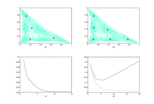
Figure 1: (a-b) 3D Probability data with 4 and 6 cluster centers, $n=8000$; (c) convergence of the $CM$ algorithm based on $KL$ divergence in the case of 6 clusters; (d) behavior of the empirical error (3) (blue, dashed) and empirical error with cost term (35) where $\alpha=0.1,\beta=0.03$.

Remark 2   As it was demonstrated in [5], cluster centers $q_{c}$ in the space $\mathcal{P}^{m}$ with $KL$-divergence must be computed using $K$-means:

$$q_{c}=\frac{1}{n_{c}}\sum_{x_{t}\in{\mathbf{X}}_{c}}p_{t}$$ (29)

where $c(x_{t})=c$ if $x_{t}\in{\mathbf{X}}_{c}$ and $n_{c}=\#{\mathbf{X}}_{c}$ is the number of observations in the cluster ${\mathbf{X}}_{c},c=1,\ldots,k$, $p_{t}=\{p_{1t},\ldots,p_{mt}\},q_{c}=\{q_{1t},\ldots,q_{mt}\}$.

In difference to the model of [11] in $\mathbb{R}^{m}$, the structure (9) covers an important case of $\mathcal{P}^{m}$ with $KL$-divergence:

$$\xi_{0}(v)=\sum_{\ell=1}^{m}v_{\ell}\log{v_{\ell}};\hskip 7.22743pt\xi_{\ell}(v)=v_{\ell};$$ (30)

$\eta_{0}(u)=1;\hskip 7.22743pt\eta_{\ell}(u)=-\log{u_{\ell}},\ell=1,\ldots,m.$

Definition. We will call element $v\in\mathcal{P}^{m}$ as 1) uniform center if $v_{\ell}=\frac{1}{m},\ell=1,\ldots,m$; as 2) absolute margin if $\min_{\ell}{v_{\ell}}=0$.

Proposition 1

The ball $B(Z)\subset\mathcal{P}^{m}$ contains only one element named as uniform center in the case if $Z={\mathbf{r}}_{0}=\log{(m)}$, and $B(Z)=\emptyset$ if $Z<{\mathbf{r}}_{0}$.

Proof: Suppose, that $u$ is a uniform center. Then, $KL(v,u)=\sum_{i=1}^{m}v_{i}\log{v_{i}}+\log{m}\leq\log{m}$ for all $v\in\mathcal{P}^{m}$. In any other case, one of the components of $u$ must be less than $\frac{1}{m}$. Respectively, we can select corresponding component of the probability vector $v$ as $1$. Therefore, $KL(v,u)>\log{(m)}$ and ${\mathbf{r}}_{0}=\log{(m)}$. $\blacksquare$

Lemma 3

The $KL$ divergence in probabilistic space $\mathcal{P}^{m}$ always satisfies condition (28) where vector-function $\xi$ is expressed by (30) with the following upper bounds:

$$|\xi_{0}(v)|\leq\log{(m)};\hskip 7.22743pt|\xi_{\ell}(v)|\leq 1,\ell=1,\ldots,m,\hskip 7.22743pt\hskip 7.22743pt\forall v\in\mathcal{P}^{m}.$$

Lemma 4

The following relations are valid in $\mathcal{P}^{m}$

1. $min_{\ell}\{u_{\ell}\}<e^{-r}$ for all $u\in T(r)\hskip 7.22743pt\forall r\geq{\mathbf{r}}_{0}$;

2. $u_{\ell}\geq e^{-r}$ for all $\ell=1,\ldots,m$, and any $u\in B(r)\hskip 7.22743pt\forall r\geq{\mathbf{r}}_{0}$.

Proof: As far as $\mathcal{P}^{m}=B(r)\cup T(r),B(r)\cap T(r)=\emptyset$, the first statement may be regarded as consequence of the second. Suppose, that $u\in B(r)$ and $u_{1}=e^{-r-\varepsilon},\varepsilon>0$. Then, we can select $v_{1}=1$, and $KL(v,u)=r+\varepsilon>r$ - contradiction. $\blacksquare$

Corollary 1

The $KL$ divergence in $\mathcal{P}^{m}$ always satisfies conditions (17) and

$$-\log{(m)}+Z\cdot e^{-r}<\rho(B(r),T(Z))\leq e^{-r}\cdot\left(Z-r\right)+\left(1-e^{-r}\right)\log{\frac{1-e^{-r}}{1-e^{-Z}}}$$

for all     ${\mathbf{r}}_{0}\leq r<Z$ where the distance $\rho$ is defined in (15).

Proof: Suppose, that $v\in B(r)$ and $u\in T(Z)$. Then, $-\sum_{i=1}^{m}v_{i}\log{(u_{i})}>Z\cdot e^{-r}$ for all     $r:{\mathbf{r}}_{0}\leq r<Z$. On the other hand, the entropy $H(v)=-\sum_{i=1}^{m}v_{i}\log{(v_{i})}$ may not be smaller comparing with $\log{(m)}$. The low bound is proved. In order to prove the upper bound we shall suppose without loss of generality that $v_{1}=e^{-r},u_{1}=e^{-Z}$, and all other components are proportional. $\blacksquare$

Theorem 2

Suppose that probability measure $\mathbb{P}$ satisfies condition (14) in probabilistic space $\mathcal{P}^{m}$ with $KL$ divergence and number of clusters $k$ is fixed. Then, the minimal empirical error (6) will converge to the minimal actual error (4) with probability 1 or a.s.

Proof: Follows directly from the Lemmas 1, 2, 3 and 4.

Remark 3   Condition (14) will not be valid if and only if a probability of the subset of all absolute margins is strictly positive. Note that in order to avoid any problems with consistency we can generalise definition of $KL$-divergence using special smoothing parameter $0\leq\theta\leq 1$:

$$KL_{\theta}(v,u)=KL(v_{\theta},u_{\theta})$$

where $v_{\theta}=\theta v+(1-\theta)v_{0}$ and $u_{\theta}=\theta u+(1-\theta)v_{0}$, $v_{0}$ is uniform center.

5 Clustering Regularization

Let us introduce the following definitions:

$${\mathbf{q}}_{c}:=\frac{1}{n_{c}}\sum_{x_{t}\in{\mathbf{X}}_{c}}p_{t};\hskip 7.22743pt{\mathbf{q}}:=\frac{1}{n}\sum_{x_{t}\in{\mathbf{X}}}p_{t}=\sum_{c=1}^{k}p_{c}\cdot{\mathbf{q}}_{c};$$

$$H({\mathbf{q}}_{c}):=-\langle{\mathbf{q}}_{c},\log{{\mathbf{q}}_{c}}\rangle;\hskip 7.22743ptH({\mathbf{X}}):=\frac{1}{n}\sum_{x_{t}\in{\mathbf{X}}}H(x_{t})$$

where $p_{c}=P({\mathbf{X}}_{c})=\frac{n_{c}}{n},c=1,\ldots,k,$ and $H(x_{t})=-\langle p_{t},\log{p_{t}}\rangle$.

We define in this section a regularisation to restrict usage of unnecessary clusters. This regularisation is based on the following two conditions:

1. $p_{c}\geq\alpha>0,c=1,\ldots,k$ (significance of any particular cluster);

2. $KLS({\mathbf{q}}_{i},{\mathbf{q}}_{c}):=KL({\mathbf{q}}_{i},{\mathbf{q}}_{c})+KL({\mathbf{q}}_{c},{\mathbf{q}}_{i})\geq\beta>0$ (difference between any 2 clusters $i$ and $c,i\neq c$).

According to [8], if more prototypes are used for the $k$-means clustering, the algorithm splits clusters, which means that it represents a single cluster by more than one prototype. The following Proposition 2 considers clustering procedure in an inverse direction.

Proposition 2

The following representations are valid

$$\Re_{\mathrm{emp}}^{(k)}=-H({\mathbf{X}})+\sum_{c}p_{c}H({\mathbf{q}}_{c});\hskip 3.61371pt\Re_{\mathrm{emp}}^{(1)}-\Re_{\mathrm{emp}}^{(k)}=\sum_{c=1}^{k}p_{c}KL({\mathbf{q}}_{c},{\mathbf{q}}),\hskip 3.61371pt\forall n\geq k\geq 1.$$

Proof: In accordance with above definitions

$$\Re_{\mathrm{emp}}^{(k)}=-H({\mathbf{X}})-\sum_{c}\frac{n_{c}}{n}\sum_{x_{t}\in{\mathbf{X}}_{c}}\frac{1}{n_{c}}\langle p(x_{t}),\log{{\mathbf{q}}_{c}}\rangle,\hskip 3.61371pt\forall k\geq 1,$$

and

$$\Re_{\mathrm{emp}}^{(1)}-\Re_{\mathrm{emp}}^{(k)}=\sum_{c}p_{c}H({\mathbf{q}}_{c})-H({\mathbf{q}})=\\ \sum_{c}p_{c}\langle{\mathbf{q}}_{c},\log{{\mathbf{q}}_{c}}-\log{{\mathbf{q}}}\rangle$$

where the second equation follows directly from the first one. $\blacksquare$

Corollary 1

Assuming that we merge first $\tau$ clusters, $1\leq\tau\leq k$, the following relation is valid

$$\Re_{\mathrm{emp}}^{(k-\tau+1)}-\Re_{\mathrm{emp}}^{(k)}\leq\sum_{c=1}^{\tau}p_{c}KL({\mathbf{q}}_{c},\widehat{{\mathbf{q}}}_{\tau}),\hskip 7.22743pt\widehat{{\mathbf{q}}}_{\tau}=\frac{\sum_{c=1}^{\tau}p_{c}{\mathbf{q}}_{c}}{\sum_{c=1}^{\tau}p_{c}}.$$ (31)

Remark 4   First $\tau$ clusters were chosen in order to simplify notifications and without loss of generality.

As a result of standard application of Jensen’s inequality to (31) we can formulate similar results in terms of particular differences between clusters.

Corollary 2

The following relation is valid

$$\Re_{\mathrm{emp}}^{(k-\tau+1)}-\Re_{\mathrm{emp}}^{(k)}\leq\frac{\sum_{i=1}^{\tau}\sum_{c=1}^{\tau}p_{i}p_{c}KL({\mathbf{q}}_{i},{\mathbf{q}}_{c})}{\sum_{c=1}^{\tau}p_{c}}$$ (32)

for any $n\geq k\geq 2$.

As a direct consequence of (32), we derive formula for the case of two clusters indexed by $i$ and $c$:

$$\Re_{\mathrm{emp}}^{(k-1)}-\Re_{\mathrm{emp}}^{(k)}\leq\frac{p_{i}\cdot p_{c}\cdot KLS(q_{i},q_{c})}{p_{i}+p_{c}}.$$ (33)

The coefficient $\frac{p_{i}\cdot p_{c}}{p_{i}+p_{c}}$ in (33) represents an increasing function of probabilities $p_{i}$ and $p_{c}\geq\alpha$. Respectively, we form regularized empirical risk by including additional $cost$ term in (6):

$$\Re^{(k)}_{\mathrm{emp}}[\mathcal{Q}_{n}]+C(k)$$ (34)

where

$$C(k)=\frac{\alpha\cdot\beta\cdot k}{2}.$$ (35)

Minimizing above regularized empirical risk as a function of number of clusters $k$ we will make required selection of the clustering size (see Figures 1(d)).

Remark 5

Note a structural similarity between (34) and Akaike Information Criterion [1] and [2], which has different grounds. In accordance with AIC, the empirical log-likelihood is greater compared with the actual log-likelihood because we use the same data in order to estimate the required parameters. Asymptotically, the bias represents a linear function of the number of the used parameters.

6 Concluding Remarks

Cluster analysis, an unsupervised learning method [13], is widely used to study the structure of the data when no specific response variable is specified. Recently, several new clustering algorithms (e.g., graph-theoretical clustering, model-based clustering) have been developed with the intention to combine and improve the features of traditional clustering algorithms. However, clustering algorithms are based on different assumptions, and the performance of each clustering algorithm depends on properties of the input dataset. Therefore, the winning clustering algorithm does not exist for all datasets, and the optimization of existing clustering algorithms is still a vibrant research area [3].

Probabilistic space with $KL$-divergence represents an essentially different case compared with Euclidean space with standard squared metric. In this paper we considered an illustration with a simple synthetic example. However, many real-life datasets may be transferred into probabilistic space as a result of the proper normalisation. For example, we know that all elements of the colon dataset are strictly positive. We can normalise any row of the colon matrix (which has interpretation as a gene) by division by the sum of the corresponding elements. As a next step, we can apply the model of Section 4 in order to reduce dimensionality of the gene expression data. This analysis has an important role to play in the discovery, validation and understanding of various classes and subclasses of cancer [9].

References

- [1] H. Akaike. “Information Theory and an extension of the maximum likelihood principle.” B.N. Petrov and F. Csaki, Proc. 2nd International Symposium on Information Theory, Akademaii-Kiado, Budapest, pp. 267-281, 1973.
- [2] H. Akaike. “On the Likelihood of a Time Series Model.” The Statistician, vol. 27, pp. 217-235, 1978.
- [3] N. Belacel, Q. Wang and M. Cuperlovic-Culf. “Clustering Methods for Microarray Gene Expression Data.” A Journal of Integrative Biology, vol. = 10(4), pp. 507-531, 2006.
- [4] J. Cuesta-Albertos, A. Gordaliza and C. Matran. “Trimmed k-Means: an Attempt to Robustify Quantizers.” The Annals of Statistics, vol. 25(2), pp. 553-576, 1997.
- [5] I. Dhillon, S. Mallela and R. Kumar. “Divisive Information-Theoretic Feature Clustering Algorithm for Text Classification.” Journal of Machine Learning Research, vol. 3, pp. 1265-1287, 2003.
- [6] C. Fraley and A. Raftery. “How many clusters? Which clustering method? Answers via model-based cluster analysis.” The Computer Journal, vol. 41(8), pp. 578-588, 1998.
- [7] G. Hamerly and C. Elkan. “Learning the k in k-means.” 16th Conference on Neural Information Processing Systems, 2003.
- [8] A. Hinneburg and D. Keim. “A General Approach to Clustering in Large Databases with Noise.” Knowledge and Information Systems, vol. 5, pp. 387-415, 2003.
- [9] Y. Liu, D. Hayes, A. Nobel and J. Marron. “Statistical Significance of Clustering for High-Dimensional, Low-Sample Size Data.” Journal of the American Statistical Association, vol. 103(483), pp. 1281-1293, 2008.
- [10] A. Ng, M. Jordan and Y. Weiss. “On spectral clustering: analysis and an algorithm.” 13th Conference on Neural Information Processing Systems, 2001.
- [11] D. Pollard. “Strong Consistency of K-Means Clustering.” The Annals of Statistics, vol. 10(1), pp. 135-140, 1981.
- [12] G. Schwarz. “Estimating the Dimension of a Model.” The Annals of Statistics, vol. 6(2), pp. 461-464, 1978.
- [13] G. Tseng and W. Wong. “Tight clustering: a resampling-based approach for identifying stable and tight patterns in data.” Biometrics, vol. 61, pp. 10-16, 2005.
- [14] V. Vapnik. “The nature of statistical learning theory.” Springer, 1995.
- [15] S. Zhong and J. Ghosh. “A Unified Framework for Model-based Clustering.” Journal of Machine Learning Research, vol. 4, pp. 1001-1037, 2003.