Tilted-Cone Induced Cusps and Nonmonotonic Structures
in Dynamical Polarization Function of Massless Dirac Fermions

Abstract

We examine the dynamical property of the polarization function for electrons with the tilted Dirac cone, considering the case where the chemical potential measured from the contact point is finite, as found in the organic conductor $\alpha$-(BEDT-TTF)₂I₃ (BEDT-TTF=bis(ethylene-dithio)tetrathiafulvalene) at ambient pressure. Using the tilted Weyl equation with the analytical treatment of the particle-hole excitation, we show that the polarization function as a function of both the frequency and the momentum exhibits cusps and nonmonotonic structures. The polarization function depends not only on the magnitude but also on the direction of the external momentum. These properties are characteristic of the tilted Dirac cone, and are in contrast to those in the isotropic case of graphene. Furthermore, the results are applied to calculate the optical conductivity, plasma frequency, and the screening of Coulomb interaction, which are also strongly influenced by the tilted cone.

1 Introduction

The recent discovery of graphene[1] has attracted much attention in the field of condensed matter because graphene exhibits massless Dirac fermions. Using the Weyl equation, [2, 3] which describes the motion of massless Dirac fermions, several anomalous electronic properties have been investigated for a long time.[5, 4] Another massless Dirac fermion is found in the quasi-two-dimensional organic conductor $\alpha$-(BEDT-TTF)₂I₃ (BEDT-TTF=bis(ethylene-dithio)tetrathiafulvalene) under pressure [6, 7]. The existence was demonstrated theoretically [8, 9] using the band calculation, which is based on the transfer integrals estimated from the X-ray structure analysis.[10] Such an energy band has been confirmed by first-principles calculations.[11, 12] This novel state elucidates a long standing problem of anomalous phenomena observed in the conductor under pressure.[13, 14]

The massless Dirac fermion in the organic conductor is expected to exhibit a noticeable property due to the anisotropic velocity of the tilted Dirac cone, which is described by the tilted Weyl equation.[15, 16, 17, 18] It has been shown that the tilt affects the characteristic temperature dependence of the Hall coefficient[19] where the magnitude of the tilt is characterized by the parameter $\alpha=v_{0}/v_{c}$ ($0\leq\alpha<1$), the ratio of the tilting velocity to the cone velocity. A recent experiment on the transport phenomena of $\alpha$-(BEDT-TTF)₂I₃ suggested that $\alpha\cong 0.8$ using theoretical evaluation.[20] Since the conductor is a layered two-dimensional massless Dirac fermion system,[21, 22] the interplane magnetoresistance also exhibits noticeable properties, as shown theoretically by the angle dependence of the magnetic field. [23] Moreover, new phenomena induced by the tilted Dirac cones have been maintained by calculating the transport coefficient under strong magnetic field, the electric-field-induced lifting of the valley degeneracy,[24] and the easy-plane pseudo-spin ferromagnet leading to the Kosterlitz-Thouless transition.[25] In addition to the above studies, dynamical properties such as electron-hole excitation and collective excitation are promizing ingredients for verifying the role of tilting. Although the electronic state has been studied extensively, the dynamical properties associated with the polarization function are not yet clear enough compared with those in the isotropic case of graphene.

In the present paper, we analytically examine the dynamical polarization function with the arbitrary wavevector and frequency, and compare it with that in the isotropic case of graphene.[26, 27, 28, 29, 30] We examine the metallic state where the contact point of the Dirac cone is located below the Fermi energy as expected for the organic conductor $\alpha$-(BEDT-TTF)₂I₃. [7, 9, 10] In §2, formulation for the polarization function is given. In §3, the analytical expression of the imaginary part is calculated, while the real part is estimated semianalytically using the Kramers-Kronig relation. In terms of these results, we demonstrate the cusps and nonmonotonic structures as characteristic of tilted Dirac cone. On the basis of the results of §3, we calculate the optical conductivity, plasma frequency, and screening of the Coulomb interaction in §4. The conclusion is given in §5.

2 Formulation

We consider the zero-gap state in $\alpha$-(BEDT-TTF)₂I₃, which has two tilted Dirac cones. [9] Among two contact points, $\pm\bm{k}_{0}$, corresponding to two valleys of cones, we focus on one of them, which is given by the state located close to $\bm{k}_{0}(=k_{0x},k_{0y})$ with $k_{0x}<0$ and $k_{0y}>0$. For such a state, the effective Hamiltonian is expressed as [15]

$$H=\sum_{\gamma\gamma^{\prime}=1,2}\left(H_{\bm{k}}\right)_{\gamma\gamma^{\prime}}a_{\gamma,{\bm{k}}}^{\dagger}a_{\gamma^{\prime},{\bm{k}}},$$ (1)

which gives the tilted Weyl equation. The quantity $a_{{\bm{k}}\gamma}^{\dagger}$ denotes a creation operator of the electron where the momentum ${\bm{k}}$ is measured from that of the contact point. The apex of the Dirac cone for the conduction band touches that of the valence band. Using the Luttinger-Kohn representation, where the two states at the contact point are chosen as the basis with the index $\gamma$, the matrix $H_{\bm{k}}$ is expressed as

$$H_{\bm{k}}={\bm{k}}\!\cdot\!\begin{pmatrix}{\bm{v}}_{0}&{\bm{v}}_{1}-i{\bm{v}}_{2}\\ {\bm{v}}_{1}+i{\bm{v}}_{2}&{\bm{v}}_{0}\end{pmatrix}.$$ (2)

Two states of the basis are chosen so as to give ${\bm{v}}_{0}=(v_{0},0),{\bm{v}}_{1}=(v,0),{\bm{v}}_{2}=(0,v^{\prime})$ with $v=v^{\prime}=v_{c}$ (we use $\hbar=1$). Diagonalizing eq. (2), the energy around the contact point is obtained as

$$\xi_{s{\bm{k}}}=v_{0}k_{x}+sv_{c}|{\bm{k}}|,\quad(s=\pm 1),$$ (3)

where the first term comes from the tilting along the $k_{x}$-direction. Defining a tilting parameter $\alpha(<1)$ as

$$\alpha=\frac{v_{0}}{v_{c}},$$ (4)

eq. (3) is rewritten as

$$\xi_{s{\bm{k}}}=(s+\alpha\cos\theta_{\bm{k}})v_{c}k,$$ (5)

where ${\bm{k}}=(k_{x},k_{y})$, $k=|{\bm{k}}|$ and $\tan\theta_{\bm{k}}=k_{y}/k_{x}$.

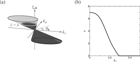
Figure 1: (a) Energy dispersion of the Dirac cone tilted along $k_{x}$-direction. The chemical potential is situated on the upper cone where the white circle denotes the Fermi surface. The angle $\theta_{\bm{k}}$, which is measured from the $k_{x}$-axis, is given by $\theta_{\bm{k}}=\arctan(k_{y}/k_{x})$ in the $k_{x}$-$k_{y}$ plane. (b)Chemical potential $\mu$ (meV) as a function of the uniaxial pressure $P_{a}$ (GPa) for $\alpha$-(BEDT-TTF)₂I₃.

From eq. (5), the trajectory for the fixed $\xi_{s,{\bm{k}}}$ gives the ellipse with a focus at $k=0$. Figure 1(a) shows the energy dispersion obtained from eq. (3) where the Dirac cone of the upper band touches that of the lower band at the contact point, $\bm{k}=0$. In the present paper, the energy is scaled by the Fermi energy (i.e., the chemical potential $\mu$), which is measured from the contact point. In Fig. 1(b), [10] the chemical potential of $\alpha$-(BEDT-TTF)₂I₃ is shown as a function of the uniaxial pressure $P_{a}$ along the a-axis. With increasing $P_{a}$ from ambient pressure, $\mu$ decreases from 7 meV and reduces to zero at $P_{a}=2.9$ kbar, above which the zero gap state is obtained. The case of $\mu=0$ is briefly mentioned in the discussion. The eigenvector for eq. (3) is given by

$${\bm{F}}_{s}(\bm{k})=\frac{1}{\sqrt{2}}\begin{pmatrix}e^{-i\theta_{\bm{k}}}\\ s\end{pmatrix}.$$ (6)

Thus, eq. (1) is rewritten as

$$\sum_{\gamma\gamma^{\prime}=1,2}\left(H_{\bm{k}}\right)_{\gamma\gamma^{\prime}}a_{\gamma,{\bm{k}}}^{\dagger}a_{\gamma^{\prime},{\bm{k}}}=\sum_{s=\pm}\xi_{s,{\bm{k}}}w_{s,{\bm{k}}}^{\dagger}w_{s,{\bm{k}}},$$ (7)

where

$$w_{s,{\bm{k}}}=\sum_{{\bm{k}}}\left({\bm{F}}_{s}({\bm{k}})\right)^{t}_{\gamma}a_{\gamma,{\bm{k}}}.$$ (8)

For these two operators, Green’s functions of the single particle are defined by

$$G_{s}({\bm{k}},{\rm i}\varepsilon_{n})=-\frac{1}{2}\int_{-1/T}^{1/T}{\rm d}\tau\left<T_{\tau}w_{s,{\bm{k}}}(\tau)w_{s,{\bm{k}}}(0)^{\dagger}\right>{\rm e}^{-{\rm i}\varepsilon_{n}\tau},$$ (9a)

$$G_{\gamma\gamma^{\prime}}^{\rm LK}({\bm{k}},{\rm i}\varepsilon_{n})=-\frac{1}{2}\int_{-1/T}^{1/T}{\rm d}\tau\left<T_{\tau}a_{\gamma,{\bm{k}}}(\tau)a_{\gamma^{\prime},{\bm{k}}}(0)^{\dagger}\right>{\rm e}^{-{\rm i}\varepsilon_{n}\tau},$$ (9b)

where $\varepsilon_{n}(={\rm i}(2n+1)\pi T)$ is the Matsubara frequency for the fermion. $T$ is the temperature and $T_{\tau}$ is the ordering operator for the imaginary time (we use $k_{\rm B}=1$) . Equation (9b) is written explicitly as

$$G^{\rm LK}=\frac{1}{({\rm i}\varepsilon_{n}-v_{0}k_{x})^{2}-v_{c}^{2}k^{2}}\begin{pmatrix}{\rm i}\varepsilon_{n}-v_{0}k_{x}&v_{c}(k_{x}-{\rm i}k_{y})\\ v_{c}(k_{x}+{\rm i}k_{y})&{\rm i}\varepsilon_{n}-v_{0}k_{x}\end{pmatrix}.$$ (10)

The polarization function per valley is calculated as

$$\Pi({\bm{q}},{\rm i}\omega_{m})= -2\sum_{\gamma\gamma^{\prime}}\int_{0}^{1/T}d\tau{\rm e}^{i\omega_{m}\tau}\big{<}T_{\tau}\rho_{\gamma,{\bm{q}}}(\tau)\rho^{\dagger}_{\gamma^{\prime},{\bm{q}}}(0)\big{>}$$

$$= -\frac{2}{\beta L^{2}}\sum_{{\bm{k}}n\gamma\gamma^{\prime}}G_{\gamma\gamma^{\prime}}^{\rm LK}({\bm{k}}+{\bm{q}},{\rm i}\varepsilon_{n}+{\rm i}\omega_{m})G_{\gamma^{\prime}\gamma}^{\rm LK}({\bm{k}},{\rm i}\varepsilon_{n})$$

$$= -\frac{2}{\beta L^{2}}\sum_{{\bm{k}}nss^{\prime}}\big{|}{\bm{F}}^{\dagger}_{s}({\bm{k}}){\bm{F}}_{s^{\prime}}({\bm{k}}+{\bm{q}})\big{|}^{2}G_{s^{\prime}}({\bm{k}}+{\bm{q}},{\rm i}\varepsilon_{n}+{\rm i}\omega_{m})G_{s}({\bm{k}},{\rm i}\varepsilon_{n}),$$ (11)

where the freedom of the spin is included. ${\rm i}\omega_{m}(={\rm i}2m\pi T)$ is the Matsubara frequency for the boson. $\rho_{\gamma,{\bm{q}}}$ is the electron density operator defined as $\rho_{\gamma,{\bm{q}}}=\sum_{{\bm{k}}}a^{\dagger}_{\gamma,{\bm{k}}}a_{\gamma,{\bm{k}}+{\bm{q}}}$ and

$$\big{|}{\bm{F}}_{s}^{\dagger}(\bm{k}){\bm{F}}_{s^{\prime}}({\bm{k}}^{\prime})\big{|}^{2}=\frac{1}{2}\Bigl{[}1+ss^{\prime}\cos(\theta_{\bm{k}}-\theta_{{\bm{k}}^{\prime}})\Bigr{]}.$$ (12)

After performing an analytical continuation given by $i\omega_{m}\longrightarrow\omega+i\eta,(\eta=+0)$, one obtains

$$\Pi({\bm{q}},\omega)= \sum_{ss^{\prime}}\left(\frac{-2}{L^{2}}\right)\sum_{{\bm{k}}}\big{|}{\bm{F}}^{\dagger}_{s}({\bm{k}}){\bm{F}}_{s^{\prime}}({\bm{k}}+{\bm{q}})\big{|}^{2}\frac{f(\xi_{s,{\bm{k}}})-f(\xi_{s^{\prime},{\bm{k}}+{\bm{q}}})}{\omega+{\rm i}\eta-(\xi_{s^{\prime},{\bm{k}}+{\bm{q}}}-\xi_{s,{\bm{k}}})}$$

$$\equiv \sum_{ss^{\prime}}\Pi_{ss^{\prime}}({\bm{q}},\omega),$$ (13)

where $f(\xi)=(1+{\rm e}^{(\xi-\mu)/T)})^{-1}$. The term $\Pi_{ss}$ comes from the electron-hole excitation of the intraband, while the term $\Pi_{s,-s}$ comes from that of the interband.

In the present paper, we examine the case for $T=0$ and calculate eq. (2) analytically by performing the integration over $\bm{k}$. The case for $\omega\geq 0$ and $\mu\geq 0$ is calculated, while the case for $\omega<0$ is obtained from

$$\Pi({\bm{q}},-\omega)=\bigl{[}\Pi(-{\bm{q}},\omega)\bigr{]}^{*},$$ (14)

which comes from the property of $\rho_{\gamma,\bm{q}}$ of the tilted cone, i.e., without inversion symmetry. In the isotropic case with inversion symmetry, one obtains $\Pi({\bm{q}},-\omega)=\bigl{[}\Pi({\bm{q}},\omega)\bigr{]}^{*}$.

Here, we note that, by taking account of the freedom of both spin and valley, the polarization function of the total system is given by

$$\Pi^{\rm total}({\bm{q}},\omega)=\Pi({\bm{q}},\omega)+\Pi(-{\bm{q}},\omega).$$ (15)

The quantity of $\Pi({\bm{q}},\omega)$ per spin and valley is calculated in §3, while charge response is calculated using $\Pi^{\rm total}({\bm{q}},\omega)$ in §4.

3 Polarization Function

3.1 Analytical calculation

We examine the imaginary part using eq. (2). By noting ${\rm Im}\Pi_{--}={\rm Im}\Pi_{+-}=0$ due to the valence band fully occupied, we calculate the remaining parts of ${\rm Im}\,\Pi_{++}$ and ${\rm Im}\,\Pi_{-+}$, which correspond to the process excited from the conduction band and valence band, respectively. After performing the tedious but straightforward calculation, we obtain the analytical results (Appendices A and B):

$${\rm Im}\,\Pi_{++}(q,\theta_{\bm{q}},\omega)=\sum_{\zeta={\rm 1A,2A,3A}}\Pi^{\prime\prime}_{\zeta},$$ (16a)

$${\rm Im}\,\Pi_{-+}(q,\theta_{\bm{q}},\omega)=\sum_{\zeta={\rm 1B,2B,3B}}\Pi^{\prime\prime}_{\zeta}.$$ (16b)

The results consist of six regions on the $q$-$\omega$ plane where the typical case with $\theta_{q}=\pi/2$ and $\alpha=0.8$ is shown in Fig. 2. These regions of 1A, 2A, 3A, 1B, 2B, and 3B are classified into two regions, A and B, corresponding to the process of intraband and interband excitations, respectively. The regions A and B are separated by a solid line expressed as

$$\omega_{\rm res}=(1+\alpha\cos\theta_{\bm{q}})v_{c}q,$$ (17)

which is called the resonance frequency. The resonance frequency is obtained owing to the nesting of the excitations with the linear dispersion, and the polarization function diverges with the chirality factor eq.(12) taking a maximum.[31] The boundary between 2A and 3A is given by $\omega_{+}$. The boundary between 2A and 1A ( 2B and 1B) is given by $\omega_{\rm A}$. The boundary between 2B and 3B is given by $\omega_{\rm B}$. These frequencies are calculated as

$$\frac{\omega_{+}(\theta_{\bm{q}})}{\mu}=\alpha\frac{v_{c}q}{\mu}\cos\theta_{\bm{q}}-\frac{2}{1-\alpha^{2}}+\sqrt{\left(\frac{v_{c}q}{\mu}\right)^{\!\!2}-\frac{4\alpha\frac{v_{c}q}{\mu}\cos\theta_{\bm{q}}}{1-\alpha^{2}}+\left(\frac{2\alpha}{1-\alpha^{2}}\right)^{\!\!2}},$$ (18)

$$\frac{\omega_{\rm A(B)}(\theta_{\bm{q}})}{\mu}=\alpha\frac{v_{c}q}{\mu}\cos\theta_{\bm{q}}+\frac{2}{1-\alpha^{2}}-(+)\sqrt{\left(\frac{v_{c}q}{\mu}\right)^{\!\!2}+\frac{4\alpha\frac{v_{c}q}{\mu}\cos\theta_{\bm{q}}}{1-\alpha^{2}}+\left(\frac{2\alpha}{1-\alpha^{2}}\right)^{\!\!2}}.$$ (19)

In the case of the isotropic Dirac cone (i.e., $\alpha=0$),[28, 29] there is a boundary given by $\omega/\mu+v_{c}q/\mu=2$ which separates 1A and 2A (1B and 2B) for the intraband (the interband). In the regions 3A and 1B, the imaginary part vanishes. In the present case of the tilted Dirac cone, the boundary between 1A and 2A exhibits a noticeable behavior characterized by the appearance of cusps for the imaginary part as shown in this section.

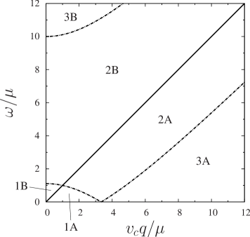
Figure 2: Several regions on the $q$-$\omega$ plane for ${\rm Im}\Pi(\bm{q},\omega)$ with the fixed $\theta_{q}=\pi/2$ and $\alpha=0.8$. The solid line denotes the resonance frequency, $\omega=\omega_{\rm res}$. The dash-dotted line between 2B and 3B corresponds to $\omega_{\rm B}$ and the line between 1A and 2A (and also 1B and 2B) corresponds to $\omega_{\rm A}$. The imaginary part is absent in the regions of both 3A and 1B. The boundary between 2A and 3A is given by $\omega_{+}$. The intersection point of $\omega_{A}$ and $\omega_{\rm res}$ is given by $v_{c}q/\mu=1/(1+\alpha\cos\theta_{\bm{q}})$ and $\omega/\mu=1$ while $\omega_{A}/\mu=2/(1+\alpha)$ at $v_{c}q/\mu=0$, and $\omega_{A}=0$ at $v_{c}q/\mu=2/(\sqrt{(1-\alpha^{2})(1-\alpha^{2}\cos^{2}\theta_{\bm{q}})}$. All the boundaries except for the solid line are followed by the cups, i.e, the jump of the derivative with respect to $q$ and $\omega$.

The real part is calculated from the imaginary part using the Kramers-Kronig relation:

$${\rm Re}\,\Pi(q,\theta_{\bm{q}},\omega)= \frac{1}{\pi}{\cal P}\int_{-\infty}^{\infty}dx\,\,\frac{{\rm Im}\,\Pi(q,\theta_{\bm{q}},x)}{x-\omega}$$

$$= \frac{1}{\pi}{\cal P}\int_{0}^{\infty}dx\,\,\frac{{\rm Im}\,\Pi(q,\theta_{\bm{q}},x)}{x-\omega}+\frac{1}{\pi}{\cal P}\int_{0}^{\infty}dx\,\,\frac{{\rm Im}\,\Pi(q,\pi+\theta_{\bm{q}},x)}{x+\omega}\;,$$ (20)

where we used, from eq. (14), the relation

$${\rm Re\,}\Pi({\bm{q}},-\omega)={\rm Re\,}\Pi(-{\bm{q}},\omega)={\rm Re\,}\Pi(q,\pi+\theta_{\bm{q}},\omega),$$

$${\rm Im\,}\Pi({\bm{q}},-\omega)=-{\rm Im\,}\Pi(-{\bm{q}},\omega)=-{\rm Im\,}\Pi(q,\pi+\theta_{\bm{q}},\omega).$$ (21)

The result of the semianalytical calculation is given in Appendix C

3.2 Behavior of the polarization function

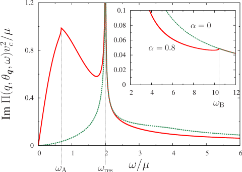
Figure 3: (Color online) Normalized imaginary part, ${\rm Im}\Pi(\theta_{\bf q},\omega)v_{c}^{2}/\mu$, as a function of $\omega/\mu$ with $q=2\mu/v_{c}$ and $\theta_{q}=\pi/2$. This behavior is expected in the case of $1/(1+\alpha\cos\theta_{\bm{q}})<v_{c}q/\mu<2/(\sqrt{1-\alpha^{2}}\sqrt{1-\alpha^{2}\cos^{2}\theta_{\bm{q}}})$. The region of $0<\omega<\omega_{\rm res}$ $(\omega>\omega_{\rm res})$ comes from the intraband (interband) excitation. The dotted line represents the isotropic case. The cusp in the intraband region is found at $\omega=\omega_{A}$, while that in the interband region is found at $\omega=\omega_{B}$ (the inset).

The imaginary part exhibits a variety of $\omega$ dependences depending on the magnitude of $\bm{q}$, which is divided into the following three regions. In the region of the small $q$, a gap exists in the interband excitation, while in the region of the large $q$ a gap exists in the intraband excitation. The intermediate region of $q$ is located between these two regions.

First, we show a novel behavior seen for the intermediate magnitude of $\bm{q}$, which comes from the tilted Dirac cone. In Fig. 3, ${\rm Im}\Pi(\theta_{\bf q},\omega)v_{c}^{2}/\mu$ with fixed $v_{c}q/\mu=2$ and $\theta_{\bm{q}}=\pi/2$ is shown as a function of $\omega/\mu$. There are two cusps at $\omega=\omega_{A}$ in the intraband region ($0<\omega<\omega_{\rm res}$) and at $\omega=\omega_{B}$ in the interband region ($\omega>\omega_{\rm res}$), where $\omega_{A}$ and $\omega_{B}$ are given by eq. (70). Note that

$$\omega_{\rm A}<\omega_{\rm res}<\omega_{\rm B},$$ (22)

since regions for intraband and interband excitations are separated by $\omega_{\rm res}$.

Here, using Fig. 4, we explain the cusp at $\omega=\omega_{A}$ in the intraband region. Equation (2) shows the following three kinds of conditions for obtaining the imaginary part. The first one is the energy conservation given by

$$\omega=\xi_{+,{{\bm{k}}+{\bm{q}}}}-\xi_{+,{\bm{k}}},$$ (23)

and the second one is the possible process of the electron-hole excitation given by $f(\xi_{+,{\bm{k}}})-f(\xi_{+,{\bm{k}}+{\bm{q}}})=1$, which leads to

$$\xi_{+,{\bm{k}}}<\mu,$$ (24)

$$\xi_{+,{\bm{k}}+{\bm{q}}}>\mu.$$ (25)

The third one, which is discussed later is a factor given by eq. (12). From the second condition, it is found that $\bm{k}$ is allowed inside of ellipse (I) and outside of ellipse (II) on the $k_{x}$-$k_{y}$ plane where ellipse (I) and ellipse (II) denote $\xi_{+,{\bm{k}}}=\mu$ and $\xi_{+,{\bm{k}}+{\bm{q}}}=\mu$, respectively. By defining R as the intersection point between ellipse (I) and $k_{y}=k_{x}\tan\theta_{\bm{q}}(>0)$, one finds $\omega=\omega_{\rm res}$ being the maximum on the line given by $k_{y}=k_{x}\tan\theta_{\bm{q}}(>0)$ (i.e., on the line OR). The cusp is understood as follows when the origin O (i.e., $k_{x}=0$ and $k_{y}=0$ ) is located outside ellipse (II). We define $P_{1}$ and $P_{2}$ as the intersection points between ellipse (I) and ellipse (II) at which $\omega(=\xi_{+,{\bm{k}}}-\xi_{+,{{\bm{k}}+{\bm{q}}}})\rightarrow 0$. Thus, $\omega$ increases from zero to $\omega_{\rm res}$ when the point moves from $P_{1}$( or $P_{2}$) to R on ellipse (I). Here, we consider ellipse (III), which has the same focus as ellipse (I) and touches ellipse (II) at the point A. It can be shown that such ellipse (III) is given by

$$\xi_{+,{\bm{k}}}=\mu-\omega_{A},$$ (26)

where $\omega_{A}(>0)$ is equal to that found in Fig. 3. By noting $\xi_{+,{\bm{k}}+{\bm{q}}}-\mu>0$ at $\bm{k}=0$, and the existence of $P_{1}$ and $P_{2}$, the condition for the cusp at $\omega_{A}$ is given by

$$\frac{1}{1+\alpha\cos\theta_{\bm{q}}}<v_{c}q/\mu<\frac{2}{\sqrt{(1-\alpha^{2})(1-\alpha^{2}\cos^{2}\theta_{\bm{q}})}},$$ (27)

where $\omega_{\rm res}>\omega_{A}>0$. On ellipse (II), $\omega$ takes a minimum at $P_{1}$ (and $P_{2}$) and a maximum at A suggesting a saddle point at A, which gives rise to the cusp. Actually, this leads to an excess contribution for the imaginary part, which becomes singular for $\omega\rightarrow\omega_{A}-0$, i.e.,

$$\delta\left({\rm Im}\Pi(q,\theta_{\bm{q}},\omega)\right)\propto-\sqrt{\omega_{A}-\omega}.$$ (28)

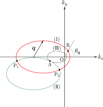
Figure 4: (Color online) Fermi surfaces for $\xi_{\bm{k}}=\mu$ (I), $\xi_{\bm{k}+\bm{q}}=\mu$ $({\rm II})$, and $\xi_{\bm{k}}=\mu-\omega_{A}$ $({\rm III})$ on the $k_{x}$-$k_{y}$ plane. Point A where I and II contact gives rise to the emergence of the cusp. $P_{1}$ and $P_{2}$ are the intersection points between ellipse (I) and ellipse (II), and O is the origin. The condition for the resonance is obtained for $k_{y}=k_{x}\tan\theta_{\bm{q}}$, which is found on the line connecting O and R.

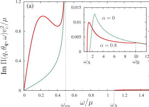
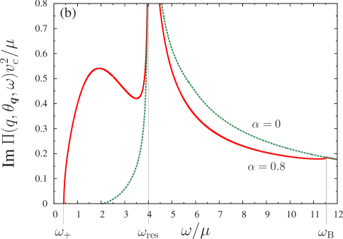
Figure 5: (Color online) Normalized imaginary part, ${\rm Im}\Pi(\theta_{\bf q},\omega)v_{c}^{2}/\mu$, as a function of $\omega/\mu$ in the case of $\theta_{q}=\pi/2$ for $q=\mu/2v_{c}$ (a) (upper panel) and for $q=4\mu/v_{c}$ (b) (lower panel). The behaviors of panels (a) and (b) are found for $v_{c}q/\mu<1/(1+\alpha\cos\theta_{\bm{q}})$ and $2/(\sqrt{1-\alpha^{2}}\sqrt{1-\alpha^{2}\cos^{2}\theta_{\bm{q}}})<v_{c}q/\mu$, respectively. The result in the isotropic case is shown by the dashed curve.

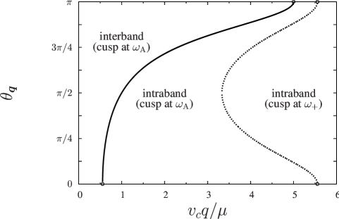
Figure 6: Region for several cusps on the $v_{c}q/\mu$ - $\theta_{\bm{q}}$ plane, where $\omega_{\rm A}$ is found for the intermediate $v_{c}q/\mu$ with the fixed $\theta_{\bm{q}}$ (eq. (27)).

Next we examine the imaginary part in the other cases of the small $q$ and the large $q$, which are found for $v_{c}q/\mu<1/(1+\alpha\cos\theta_{\bm{q}})$ and $2/(\sqrt{1-\alpha^{2}}\sqrt{1-\alpha^{2}\cos^{2}\theta_{\bm{q}}})<v_{c}q/\mu$, respectively. These examples are shown in Figs. 5(a) and 5(b) by choosing $q=\mu/2v_{c}$ (a) (upper panel) and $q=4\mu/v_{c}$ (b) (lower panel). Note that the cusp is also found at $\omega_{A}$ or $\omega_{+}$, which can be understood from the saddle point similar to that in Fig. 4. There is a broad peak for $\omega<\omega_{\rm res}$, which is also characteristic of a tilted cone and is absent in the isotropic case. The location of such a peak is almost proportional to $q$. A noticeable difference is seen between the small $q$ and the large $q$ (i.e., between the case $q=\mu/2v_{c}$ and that of $q=4\mu/v_{c}$). For $q=\mu/2v_{c}$ (upper panel), the interband contribution of ${\rm Im}\Pi(\theta_{\bf q},\omega)v_{c}^{2}/\mu$ is very small and increases from zero with increasing $\omega(>\omega_{\rm A})$. As seen from Figs. 3 and 5 (a), ${\rm Im}\Pi(\theta_{\bf q},\omega)$ of the intraband excitation ($\omega<\omega_{\rm res}$) is much larger than that of the interband excitation ($\omega>\omega_{\rm res}$). An opposite behavior emerges when $v_{c}q/\mu>>1$ (Fig. 5 (b)). For $q=4\mu/v_{c}$ (lower panel), the interband contribution of ${\rm Im}\Pi(\theta_{\bm{q}},\omega)v_{c}^{2}/\mu$ is large and is close to $\omega\sim\omega_{\rm res}$. Compared with that in the isotropic case, the intraband contribution is enhanced but the interband contribution is suppressed. Such a fact may be ascribed to a sum rule given by $\int_{0}^{\Lambda}{\rm d}\omega\omega{\rm Im}\Pi(\bm{q},\omega)=(1/8)q^{2}\Lambda$, where $\Lambda$ is the upper cutoff of the frequency. [32] For $v_{c}q/\mu<1/(1+\alpha\cos\theta_{\bm{q}})$, where $\omega_{A}>\omega_{\rm res}$, the imaginary part is absent in the interval range of $\omega_{\rm res}<\omega<\omega_{A}$. For a small $\omega$, the imaginary part is convex downward in the isotropic case owing to the absence of the backward scattering, while it is convex upward in the tilted case owing to $P_{1}$ and $P_{2}$ located away from the backward scattering. Note that the cusp at $\omega_{B}$ is present for the arbitrary $q$, as seen from Fig. 3.

We examine the $\theta_{\bf{q}}$ dependence of the imaginary part. On the basis of eq. (27), the region for the existence of $\omega_{A}$ is shown on the $v_{c}q/\mu$-$\theta_{q}$ plane in Fig. 6. The behavior for the fixed $\theta_{\bf{q}}(=\pi/2)$ is as follows. In the region for the small $v_{c}q/\mu$, the cusp at $\omega=\omega_{A}$ appears in the interband process (Fig. 5(a)), while in the middle region with an intermediate $v_{c}q/\mu$, $\omega_{A}$ exists in the intraband process (Fig. 3). For the large $v_{c}q/\mu$, the cusp appears at $\omega_{+}$, which is the lower bound of the imaginary part (Fig. 5 (b)). Note that the cusp is found, except for $\theta_{\bm{q}}=0$ and $\pi$.

Here, we briefly mention the $\theta_{\bf q}$ dependences on $\omega_{\rm A}$, $\omega_{\rm res}$, and $\omega_{\rm B}$ with a fixed $v_{c}q/\mu$. With increasing $\theta_{q}$ from zero to $\pi$, both $\omega_{\rm B}$ and $\omega_{\rm res}$ decrease monotonically, but $\omega_{\rm A}$ remains almost constant until $\omega_{A}=\omega_{\rm res}$. The cusp at $\omega_{\rm A}$ moves from the intraband region to the interband region, where the boundary is given by $\omega_{\rm res}$. Those frequencies also depend on the degree of tilting, $\alpha$. With increasing $\alpha$ from zero to 1, both $\omega_{\rm A}$ and $\omega_{\rm B}$ increase monotonically. The resonance frequency $\omega_{\rm res}$ increases (decreases) for $0<\theta_{\bf q}<\pi/2$ ($\pi/2<\theta_{\bf q}<\pi)$ with increasing $\alpha$, while $\omega_{\rm res}$ at $\theta_{\bf q}=\pi/2$ is independent of $\alpha$.

Figure 7 shows the normalized imaginary part ${\rm Im}\Pi(\theta_{\bf q},\omega)v_{c}^{2}/\mu$ on the plane of $v_{c}q/\mu$ and $\omega/\mu$ for $\theta_{\bm{q}}=$ 0(a), $\pi/2$(b), and $\pi$ (c). The color gauge with the gradation represents the magnitude of the imaginary part. The global feature is mainly determined by the property of $\omega_{\rm res}$. In the case of $v_{c}q/\mu>>1$ where the characteristic energy becomes much larger than the interband energy ($\sim\mu$), ${\rm Im}\Pi(\theta_{\bf q},\omega)$ of the intraband excitation ($\omega<\omega_{\rm res}$) becomes much smaller than that of the interband excitation ($\omega>\omega_{\rm res}$) in contrast to the case where $v_{c}q/\mu=2$ (Fig. 3). The broad peak in the intraband excitation (i.e., $\omega<\omega_{\rm res}$) does not change much for $\theta_{\bm{q}}<\pi/2$, while it is strongly masked for $\pi/2<\theta_{\bm{q}}<\pi$ due to the rapid decreasing $\omega_{\rm res}$.

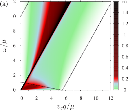
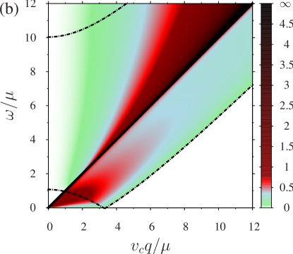
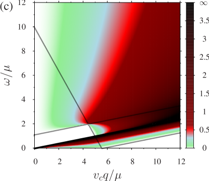
Figure 7: Normalized imaginary part, ${\rm Im}\Pi(\theta_{\bf q},\omega)v_{c}^{2}/g_{s}\mu$ on the plane of $v_{c}q/\mu$ and $\omega/\mu$ for $\theta_{q}=0$ (a), $\theta_{q}=\pi/2$ (b), and $\theta_{q}=\pi$ (c), where $\alpha=0.8$. The straight line including the origin represents the resonance frequency $\omega_{\rm res}$. The dark (bright) area represents the large (small) ${\rm Im}\Pi(\theta_{\bf q},\omega)$, while ${\rm Im}\Pi(\theta_{\bf q},\omega)=0$ in the white area corresponding to the regions of 3A and 1B in Fig. 2. The dash-dotted line (dotted line) denotes the boundary for the excitation process at which the cusp emerges (is absent).

The cusp at $\omega=\omega_{A}$ is seen for $0<\theta_{\bm{q}}<\pi$, as seen also from the analytical condition of eq. (27). The cusp in the interband process does exist in an intermediate region of $q$ for the arbitrary $\theta_{\bm{q}}$ (except for 0 and $\pi$).

Finally in this subsection, we examine the real part, which is calculated using eq. (20) (Appendix C). The numerical results of ${\rm Re}\Pi(q,\theta_{\bm{q}},\omega)v_{c}^{2}/\mu$ corresponding to the imaginary part of Figs. 3, 5(a), and 5(b) are shown in Fig. 8. When $q>(\mu/v_{c})/(1+\alpha\cos\theta_{\bm{q}})$ as seen from Figs. 8(a) and 8(c), ${\rm Re}\Pi(q,\theta_{\bm{q}},\omega)$ diverges for $\omega\rightarrow\omega_{\rm res}-0$. The cusp found in the imaginary part also appears in the real part, e.g., $\omega_{\rm A}$ and $\omega_{\rm B}$ for $v_{c}q/\mu=2$, $\omega_{\rm B}$ for $v_{c}q/\mu=1/2$, and $\omega_{+}$ and $\omega_{\rm B}$ for $v_{c}q/\mu=4$. A noticeable difference compared with the isotropic case is the nonmonotonic behavior for $\omega<\omega_{\rm res}$ and $v_{c}q/\mu>2/(1+\alpha\cos\theta_{\bm{q}})$, e.g., exhibiting a minimum for $v_{c}q/\mu=$ 2 and 4. In the regime of the interband ( $\omega>\omega_{\rm res}$), the real part is similar but is slightly small compared with that in the isotropic case.

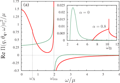
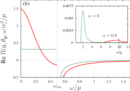
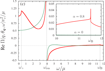
Figure 8: (Color online) Real part Re$\Pi(q,\theta_{\bm{q}},\omega)$ as a function of $\omega/\mu$ with a fixed $\theta_{\bm{q}}=\pi/2$, for $qv_{c}/\mu$ = 2 (a), 1/2(b), and 4(c), which correspond to Figs. 3 and 5(a) and 5(b). The global feature with arbitrary $q$ is seen for $\omega>\omega_{\rm res}$. The divergence of the real part for $\omega\rightarrow\omega_{\rm res}-0$ is obtained for $q>1/(1+\alpha\cos\theta_{q})$. The dotted line represents the isotropic case of graphene.

4 Optical Conductivity, Plasma Mode, and Screening Effect

4.1 Optical conductivity

The optical conductivity is obtained from two kinds of electron-hole excitations, i.e., the intraband processes and interband processes. The intraband excitation gives a Drude-like behavior in the presence of the impurity scattering, while the interband excitation gives a gaplike behavior. In this subsection, we calculate the interband optical conductivity, while the effect of the intraband one is left for discussion.

In terms of the imaginary part of $\Pi({\bm{q}},\omega)$, the optical conductivity $\sigma(\omega)$ is calculated as [33]

$$\sigma(\omega)=\lim_{q\rightarrow 0}\frac{ie^{2}\omega}{\hbar q^{2}}\left\{\Pi({\bm{q}},\omega)+\Pi(-{\bm{q}},\omega)\right\},$$ (29)

where the RPA gives the same result. Since ${\rm Im}\,\Pi(0,\omega)$ becomes finite only for the interband electron-hole excitation, ${\rm Re}\,\sigma(\omega)$ is calculated as (Appendix A)

$${\rm Re}\,\sigma(\omega)= 0\cdot\Theta\left(\frac{2\mu}{1+\alpha}-\omega\right)$$

$$+ \frac{e^{2}}{8\pi\hbar}\Biggl{[}\pi+{\rm sgn}\left(\frac{2\mu}{1+\alpha|\cos\theta_{\bm{q}}|}-\omega\right)G_{<}(z_{2}^{+})+{\rm sgn}\left(\frac{2\mu}{1-\alpha|\cos\theta_{\bm{q}}|}-\omega\right)G_{<}(-z_{2}^{-})\Biggr{]}$$

$$\times\Theta\left(\frac{2\mu}{1-\alpha}-\omega\right)\Theta\left(\omega-\frac{2\mu}{1+\alpha}\right)$$

$$+ \frac{e^{2}}{8\pi\hbar}2\pi\Theta\left(\omega-\frac{2\mu}{1-\alpha}\right),$$ (30)

where $\Theta$ is a step function, $G_{<}(x)=x\sqrt{1-x^{2}}-\arccos(x)\quad{\rm for}\quad|x|<1$, and $z_{2}^{\pm}$ are defined by

$$z_{2}^{\pm}=\frac{|\cos\theta_{\bm{q}}|}{\alpha}\left(\frac{2\mu}{\omega}-1\right)\pm\frac{|\sin\theta_{\bm{q}}|}{\alpha}\sqrt{\alpha^{2}-\left(\frac{2\mu}{\omega}-1\right)^{\!\!2}}.$$ (31)

In Fig. 9, the normalized optical conductivity ${\rm Re}\sigma(\theta_{q},\omega)4\hbar/e^{2}$ is shown as a function of $\omega/\mu$ for $\theta_{\bm{q}}=0$, $\pi/4$ and $\pi/2$, respectively, with $\alpha=0.8$. The dotted line corresponds to the isotropic case where the normalized ${\rm Re}\sigma(\theta_{\bm{q}},\omega)$ is zero for $\omega<\mu$ and is constant for $\mu<\omega$. The conductivity ${\rm Re}\sigma(\theta_{\bm{q}},\omega)$ is zero for $\omega<2\mu/(1+\alpha)$ and 1 for $\omega>2\mu/(1-\alpha)$, while it takes an intermediate value for $2\mu/(1+\alpha)<\omega<2\mu/(1-\alpha)$. The reason for such a behavior is illustrated in Figs. 10(a) and 10(b). The electron-hole excitation for the conductivity is a vertical transition from the valence band to the conduction band due to $q=0$. Figure 10(a) denotes the process with a fixed energy $\omega=\xi_{+\bm{k}}-\xi_{-\bm{k}}$. The contour projected on the $k_{x}$-$k_{y}$ plane is shown by a circle in Fig. 10(b). The ellipse of the thick line denotes the Fermi surface with $\xi=\mu$. The electron-hole excitation is allowed outside of the thick line since the hole is created above the Fermi surface of the conduction band. Thus, the process is completely forbidden for $\omega<2\mu/(1+\alpha)$, while such a process occurs on all the corresponding circles for $\omega>2\mu/(1-\alpha)$. In the intermediate case of $2\mu/(1+\alpha)<\omega<2\mu/(1-\alpha)$, the electron-hole excitation occurs on the partial part of the circles outside the thick line, i.e., for $\theta_{\bm{q}}$ satisfying the condition $\omega>2\mu/(1+\alpha\cos\theta_{\bm{q}})$. The tilting of the Dirac cone is essential for the optical conductivity that depends on $\theta_{\bm{q}}$ .

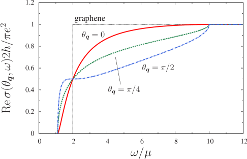
Figure 9: (Color online) Normalized interband optical conductivity ${\rm Re}\sigma(\theta_{q},\omega)2h/\pi e^{2}$ as a function of $\omega/\mu$ for $\theta_{\bm{q}}$ = 0, $\pi/4$ and $\pi/2$. The contribution comes from only the interband excitation. Note that ${\rm Re}\sigma(\theta_{\bm{q}})={\rm Re}\sigma(\pi-\theta_{\bm{q}}).$ The dotted line followed by a jump represents the isotropic case of graphene.

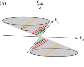
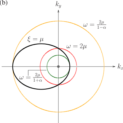
Figure 10: (Color online) (a) Particle-hole excitation with zero momentum transfer from the lower cone to the upper cone where three kinds of ellipses lead to the energy with $\omega=2\mu/(1+\alpha)$, 2$\mu$ and 2 $\mu/(1-\alpha)$. (b) The three kinds of ellipses of (a) are projected on the $k_{x}$-$k_{y}$ plane. The excitation is allowed only in the region which is located outside the Fermi surface (solid ellipse).

The conductivity can be calculated directly by taking the limit of $q\rightarrow 0$ in the imaginary part of the dielectric function. From eq. (2), the polarization function, which includes the excitation from the valence band to the conduction band is written as

$$\Pi_{-+}({\bm{q}},\omega) =-\frac{2}{(2\pi)^{2}}\int{\rm d}{\bm{k}}\left\{1-\frac{{\bm{k}}\!\cdot\!({\bm{k}}+{\bm{q}})}{|{\bm{k}}||{\bm{k}}+{\bm{q}}|}\right\}\frac{1-f(\xi_{+,\bm{k}})}{\omega+i\eta+\xi_{{-,\bm{k}}-{\bm{q}}}-\xi_{+,\bm{k}}}.$$ (32)

By expanding up to $O$($q^{2}$), the imaginary part for the small $|{\bm{q}}|$ is rewritten as

$${\rm Im}\,\Pi_{-+}({\bm{q}},\omega) \rightarrow\frac{4\pi}{(2\pi)^{2}}\int{\rm d}\varphi\int{\rm d}k\,k\frac{1-\cos^{2}(\varphi-\theta_{\bm{q}})}{4v_{c}k^{2}}q^{2}$$

$$\times\delta\left(\frac{\omega}{v_{c}}-2k-\alpha q_{x}-q\cos(\varphi-\theta_{\bm{q}})\right)\Theta\left(k+\alpha k\cos\varphi-\frac{\mu}{v_{c}}\right)$$

$$= \frac{q^{2}}{\omega}\frac{\pi}{(2\pi)^{2}}\int{\rm d}\varphi\left\{1-\cos^{2}(\varphi-\theta_{\bm{q}})\right\}\Theta\left(\omega-\frac{2\mu}{1+\alpha\cos\varphi}\right)$$

$$\equiv \frac{q^{2}}{4\omega}F_{c}(\theta_{\bm{q}}).$$ (33)

The quantity $F_{c}({\bm{q}})$ is zero for $\omega<2\mu/(1+\alpha)$ and $F_{c}({\bm{q}})=1$ for $2\mu/(1-\alpha)<\omega$, and

$$F_{c}(\theta_{\bm{q}})= \frac{1}{\pi}\int_{-\varphi_{0}}^{\varphi_{0}}{\rm d}\varphi\left\{1-\cos^{2}(\varphi-\theta_{\bm{q}})\right\}$$

$$= \frac{1}{\pi}\left(\varphi_{0}-\frac{1}{2}\sin 2\varphi_{0}\cos 2\theta_{\bm{q}}\right)$$ (34)

for $2\mu/(1+\alpha)<\omega<2\mu/(1-\alpha)$, where

$$\cos\varphi_{0}=\frac{1}{\alpha}\left(\frac{2\mu}{\omega}-1\right).$$ (35)

Thus, we obtain the optical conductivity as

$$\sigma(\omega)=\frac{e^{2}}{4\hbar}F_{c}(\theta_{\bm{q}}).$$ (36)

One finds the following $\theta_{\bm{q}}$ dependence of the optical conductivity in the interval region of $2\mu/(1+\alpha)<\omega<2\mu/(1-\alpha)$. From eq. (4.1), $\sigma$ with a fixed $\omega$ takes a maximum (minimum) at $\theta_{\bm{q}}=\pi/2$ and a minimum (maximum) at $\theta_{\bm{q}}=0$ and $\pi$ for $\omega<2\mu\,(\omega>2\mu)$.

4.2 Plasma mode

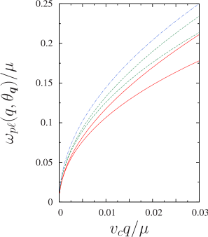
Figure 11: (Color online) Plasma frequency as a function of $v_{c}q/\mu$ for $\theta_{\bm{q}}=\pi/2,\pi/4,3\pi/4,0,\pi$ (from the top to the bottom).

We examine the plasma frequency by adding the Coulomb interaction. Within the RPA, the plasma frequency can be calculated from the pole of the polarization function, which is obtained by

$$1+v_{\bm{q}}{\rm Re}\,\Pi(q,\theta_{\bm{q}},\omega)=0,$$ (37)

where $v_{\bm{q}}$ is the Fourier transform of the Coulomb interaction,

$$v_{\bm{q}}=\frac{2\pi e^{2}}{\epsilon_{0}|{\bm{q}}|}\;.$$ (38)

Equation (37) is written explicitly as

$$1 =-v_{\bm{q}}\frac{2}{L^{2}}\sum_{{\bm{k}},s=+,s^{\prime}=+}\big{|}{\bm{F}}^{\dagger}_{s}({\bm{k}}){\bm{F}}_{s^{\prime}}({\bm{k}}+{\bm{q}})\big{|}^{2}\frac{f(\xi_{s{\bm{k}}})-f(\xi_{s^{\prime}{\bm{k}}+{\bm{q}}})}{\omega+i\eta-(\xi_{s^{\prime}{\bm{k}}+{\bm{q}}}-\xi_{s{\bm{k}}})}$$

$$=-v_{\bm{q}}\frac{1}{(2\pi)^{2}}\int_{0}^{\omega}{\rm d}k\,k\int_{0}^{2\pi}{\rm d}\varphi f(\xi_{\bm{k}})$$

$$\times\left[\left\{1+\frac{{\bm{k}}\!\cdot\!({\bm{k}}+{\bm{q}})}{|{\bm{k}}||{\bm{k}}+{\bm{q}}|}\right\}\frac{1}{\omega+\xi_{\bm{k}}-\xi_{{\bm{k}}+{\bm{q}}}}-\left\{1+\frac{{\bm{k}}\!\cdot\!({\bm{k}}-{\bm{q}})}{|{\bm{k}}||{\bm{k}}-{\bm{q}}|}\right\}\frac{1}{\omega-\xi_{\bm{k}}+\xi_{{\bm{k}}+{\bm{q}}}}\right]\;,$$ (39)

which is calculated using the real part of $\Pi(q,\theta_{\bm{q}},\omega)$ obtained in §3. In Fig. 11, plasma frequency as a function of $v_{c}q/\mu$ is shown with several choices of $\theta_{\bm{q}}$. In order to understand the behavior with a small $q$, we calculate the collective mode by expanding eq. (4.2) in terms of ${\bm{q}}$. The lowest order is obtained as

$$\omega^{2}=\frac{2\mu e^{2}}{\epsilon_{0}}C(\theta_{\bm{q}})|{\bm{q}}|\;,$$ (40)

where the coefficient $C(\theta_{\bm{q}})$ is given by

$$C(\theta_{\bm{q}}) =\frac{1}{\pi}\int_{0}^{2\pi}{\rm d}\varphi\frac{1-\cos^{2}(\varphi-\theta_{\bm{q}})}{1+\alpha\cos\varphi}$$

$$=\frac{2}{1+\sqrt{1-\alpha^{2}}}\left[1+\frac{\alpha^{2}\sin^{2}\theta_{\bm{q}}}{\sqrt{1-\alpha^{2}}(1+\sqrt{1-\alpha^{2}})}\right].$$ (41)

In this case, the plasma frequency takes a minimum, $2/(1+\sqrt{1-\alpha^{2}})$, at $\theta_{\bm{q}}$ = 0 and $\pi$, and a maximum , $2/(\sqrt{1-\alpha^{2}}(1+\sqrt{1-\alpha^{2}}))$, at $\theta_{\bm{q}}=\pi/2$. The plasma frequency in Fig. 11 reduces to the result in eq. (4.2) in the limit of a small $q$. The global behavior including a large $q$ is reported in a separate paper.

4.3 Screening of Coulomb interaction

We examine the static screening in the presence of Coulomb interaction. In the static case, i.e., $\omega=0$, the effective interaction within the RPA is given by

$$v^{\rm RPA}(q,\theta_{\bm{q}},0)=\frac{v_{\bm{q}}}{1+v_{\bm{q}}\Pi(q,\theta_{\bm{q}},0)}.$$ (42)

The real part of $\Pi(q,\theta_{\bm{q}},0)$ is shown in Fig. 12 with the fixed $\theta_{\bm{q}}=0,\pi/4$ and $\pi/2$ where the isotropic case is also shown by the dotted line. There is a cusp at $2k_{\rm F}(\theta_{\bm{q}})$ (except for $\theta_{\bm{q}}=0$), which is given by

$$k_{\rm F}(\theta_{\bm{q}})=\frac{\mu/v_{c}}{\sqrt{(1-\alpha^{2})(1-\alpha^{2}\cos^{2}\theta_{\bm{q}})}}.$$ (43)

For $q<2k_{\rm F}(\theta_{\bm{q}})$, $\Pi(q,\theta_{\bm{q}},0)$ remains constant as found in the conventional two-dimensional electron gas. In this regime, the interaction is screened as

$$v^{\rm RPA}(q,\theta_{\bm{q}},0)\rightarrow 2\pi e^{2}/\{\epsilon_{0}(q+q_{\rm TF})\},$$ (44)

where $q_{\rm TF}$ is the Thomas-Fermi screening constant given by $2e^{2}/\{\epsilon_{0}(1-\alpha^{2})^{3/2}\}$. For a large $q$, we obtain

$$\Pi(q,\theta_{\bm{q}},0)\rightarrow\frac{q}{8\sqrt{1-\alpha^{2}\cos^{2}\theta_{\bm{q}}}},$$ (45)

which corresponds to $\mu=0$ in eq. (72). In the case of a large $q$, the property of the Coulomb interaction remains with the the dielectric constant replaced by

$$\epsilon_{0}+\frac{\pi e^{2}}{4v_{c}\sqrt{1-\alpha^{2}\cos^{2}\theta_{\bm{q}}}}.$$ (46)

The dielectric constant takes a maximum (minimum ) at $\theta_{\bm{q}}=0(\pi/2)$ suggesting a fact that the anisotropy of the velocity gives rise to the enhancement of the charge response. Thus, we found that the effect of the tilted cone also emerges in the $\theta_{\bm{q}}$ dependence of the dielectric constant.

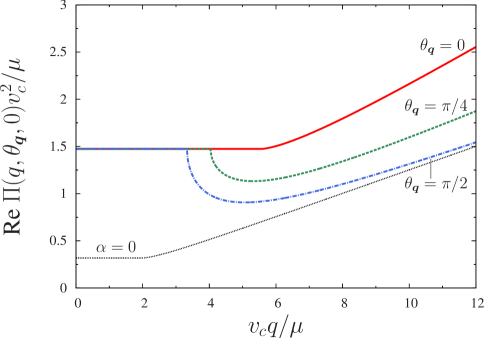
Figure 12: (Color online) Real part at $\omega=0$ as a function of $v_{c}q/\mu$ with fixed $\theta_{\bm{q}}=0,\pi/4,\pi/2$, where the lowest line denotes the result of the isotropic case of graphene.

5 Conclusions

We have examined the property of the polarization function of the massless Dirac particle with the tilted cone and a finite doping. Using the tilted Weyl equation, the dynamical polarization function with the external momentum $\bm{q}$ and frequency $\omega$ is treated analytically, and is applied to calculate the optical conductivity, plasma frequency, and screening of the Coulomb interaction. The tilting of the Dirac cone gives the following effects on the polarization function, which is determined by the intraband and interband excitations.

Several cusps as a function of the frequency, $\omega$, exist in both the imaginary part and real part of the polarization function at the characteristic frequencies, $\omega=\omega_{A}$, $\omega_{B}$, and $\omega_{+}$, depending on the momentum $\bm{q}$ and the tilting parameter $\alpha$. Nonmonotonic structures and cusps originate from the tilting and are in contrast to those in the isotropic case ($\alpha=0$). The cusps are understood in terms of the saddle point of the particle-hole excitation energy on the plane of the momentum. The tilting effect also appears in the anisotropy of the resonance frequency $\omega_{\rm res}$, which separates the intraband excitation from that of interband one. The intensity of ${\rm Im}\Pi(\theta_{\bf q},\omega)$ exhibits a strong asymmetry between the intraband region and the interband region. In the case of $v_{c}q/\mu<1$, ${\rm Im}\Pi(\theta_{\bf q},\omega)$ of the intraband excitation ($\omega<\omega_{\rm res}$) is much larger than that of the interband excitation ($\omega>\omega_{\rm res}$), while the behavior is opposite for $v_{c}q/\mu>>1$.

The optical conductivity, which is finite above the critical frequency increases continuously from zero and reaches a universal value. The plasma frequency for a small $q$, which is proportional to $q^{1/2}$, depends on $\theta_{\bm{q}}$, and is symmetric with respect to $\theta_{\bm{q}}=\pi/2$, where the coefficient takes a maximum at $\theta_{\bm{q}}=\pi/2$. Such an anisotropy also exists in the screening of the Coulomb interaction, where the renormalized dielectric constant becomes largest at $\theta_{\bm{q}}=0$. The effect of interaction on two tilted cones is reported in a separate paper within RPA.

We comment on the characteristic energy relevant to $\alpha$-(BEDT-TTF)₂I₃. It is expected that several cusps obtained in the present paper occur for the energy around the Fermi energy being $\sim$ 5 meV. However, the observation of these cusps is not straightforward since the neutron scattering is inapplicable owing to the absence of magnetic ordering and the energy scale for the X-ray experiment is too high. One possible way is to use the electromagnetic wave between microwaves and infrared waves. The optical conductivity (Fig. 9), which is obtained in the zero limit of momentum, also exhibits cusps which are different from those of $\omega_{A}$, $\omega_{B}$, and $\omega_{+}$. For the frequency dependence of the optical conductivity, the Drude like behavior of the intraband optical conductivity is well separated from the interband one since the energy for the impurity scattering ($\simeq$ 0.1 meV) is much smaller than the Fermi energy ($\simeq$ 5 meV). This is in contrast to the case of the graphene where the Drude like contribution becomes large in addition to the interband one [34] owing to the large scattering energy of 10 meV. [35] Thus, we may find the behavior showing that the optical conductivity increases continuously from the lower edge of $\hbar\omega=2\mu/(1+\alpha)$ ( $\sim$ 5 meV) and that the steep increase of the conductivity at the edge depends on $\theta_{\bm{q}}(\not=0)$. In addition to such a continuous variation, we may expect the effect of finite temperature. Although it is similar to Fig. 9, it can be distinguished from it since it approaches tangentially to the limiting value. Furthermore, there are also contributions from other two bands located around $\sim$ 500 meV below the Fermi energy ,[9] where a similar variation with respect to the frequency is expected.

Finally, we briefly mention the case of the zero gap state under pressure in which the Fermi energy is located on the contact point of the cones (i.e., $\mu\rightarrow 0$). Although the effect of tilting still existsts, through the anisotropy of $\omega_{\rm res}=(1+\alpha\cos\theta_{\bm{q}})$, $\Pi({\bm{q},\omega})$ in Fig. 2 remains finite only in a single region of the interband, i.e., $\omega_{B}$ moves to $\omega_{\rm res}$. The optical conductivity becomes constant for both the arbitrary $\omega$ and $\theta_{\bm{q}}$, while the plasma mode vanishes owing to the absence of the Fermi surface, as seen from eq. (40).

Appendix A Calculation of the Imaginary Part

By noting that $f(\xi_{s,{\bm{k}}})\rightarrow\Theta(\mu-\xi_{s,{\bm{k}}})$ for $T\rightarrow 0$ and using $(x+i\eta)^{-1}={\cal P}\frac{1}{x}-i\pi\delta(x)$, the imaginary part of eq. (2) is rewritten as

$${\rm Im}\,\Pi({\bm{q}},\omega)=\sum_{ss^{\prime}}\Pi_{ss^{\prime}}$$

$$= \frac{1}{4\pi}\!\int\!\!d{\bm{k}}\big{|}{\bm{F}}^{\dagger}_{+}({\bm{k}}){\bm{F}}_{+}({\bm{k}}+{\bm{q}})\big{|}^{2}\Bigl{[}\Theta(\mu-\xi_{+,{\bm{k}}})-\Theta(\mu-\xi_{+,{\bm{k}}+{\bm{q}}})\Bigr{]}\delta\bigl{(}\omega+\xi_{+,{\bm{k}}}-\xi_{+,{\bm{k}}+{\bm{q}}}\bigr{)}$$

$$+ \frac{1}{4\pi}\!\int\!\!d{\bm{k}}\big{|}{\bm{F}}^{\dagger}_{-}({\bm{k}}){\bm{F}}_{-}({\bm{k}}+{\bm{q}})\big{|}^{2}\Bigl{[}\Theta(\mu-\xi_{-,{\bm{k}}})-\Theta(\mu-\xi_{-,{\bm{k}}+{\bm{q}}})\Bigr{]}\delta\bigl{(}\omega+\xi_{-,{\bm{k}}}-\xi_{-,{\bm{k}}+{\bm{q}}}\bigr{)}$$

$$+ \frac{1}{4\pi}\!\int\!\!d{\bm{k}}\big{|}{\bm{F}}^{\dagger}_{+}({\bm{k}}){\bm{F}}_{-}({\bm{k}}+{\bm{q}})\big{|}^{2}\Bigl{[}\Theta(\mu-\xi_{+,{\bm{k}}})-\Theta(\mu-\xi_{-,{\bm{k}}+{\bm{q}}})\Bigr{]}\delta\bigl{(}\omega+\xi_{+,{\bm{k}}}-\xi_{-,{\bm{k}}+{\bm{q}}}\bigr{)}$$

$$+ \frac{1}{4\pi}\!\int\!\!d{\bm{k}}\big{|}{\bm{F}}^{\dagger}_{-}({\bm{k}}){\bm{F}}_{+}({\bm{k}}+{\bm{q}})\big{|}^{2}\Bigl{[}\Theta(\mu-\xi_{-,{\bm{k}}})-\Theta(\mu-\xi_{+,{\bm{k}}+{\bm{q}}})\Bigr{]}\delta\bigl{(}\omega+\xi_{-,{\bm{k}}}-\xi_{+,{\bm{k}}+{\bm{q}}}\bigr{)},$$ (47)

where ${\rm Im}\,\Pi_{--}=0$ and ${\rm Im}\,\Pi_{+-}=0$ owing to $\mu>0$. ${\bm{k}}+{\bm{q}}\rightarrow={\bm{k}}^{\prime}$ in ${\rm Im}\,\Pi_{++}$ and ${\rm Im}\,\Pi_{-+}$. By making use of eqs. (3) and (12), eq. (47) is written as

$${\rm Im}\,\Pi_{++}= \frac{1}{2\pi v_{c}}\!\int\!\!d{\bm{k}}\frac{1}{2}\Bigl{[}1+\cos(\theta_{\bm{k}}-\theta_{{\bm{k}}+{\bm{q}}})\Bigr{]}\Theta\biggl{(}\frac{\mu}{v_{c}}-k-\alpha k_{x}\biggr{)}\delta\biggl{(}\frac{\omega-v_{0}q_{x}}{v_{c}}+k-|{\bm{k}}+{\bm{q}}|\biggr{)}$$

$$- \frac{1}{2\pi v_{c}}\!\int\!\!d{\bm{k}}\frac{1}{2}\Bigl{[}1+\cos(\theta_{\bm{k}}-\theta_{{\bm{k}}-{\bm{q}}})\Bigr{]}\Theta\biggl{(}\frac{\mu}{v_{c}}-k-\alpha k_{x}\biggr{)}\delta\biggl{(}\frac{\omega-v_{0}q_{x}}{v_{c}}-k+|{\bm{k}}-{\bm{q}}|\biggr{)},$$ (48a)

$${\rm Im}\,\Pi_{-+}= \frac{1}{2\pi v_{c}}\!\int\!\!d{\bm{k}}\frac{1}{2}\Bigl{[}1-\cos(\theta_{\bm{k}}-\theta_{{\bm{k}}-{\bm{q}}})\Bigr{]}\Theta\biggl{(}k+\alpha k_{x}-\frac{\mu}{v_{c}}\biggr{)}\delta\biggl{(}\frac{\omega-v_{0}q_{x}}{v_{c}}-k-|{\bm{k}}-{\bm{q}}|\biggr{)}.$$ (48b)

Using the relation

$$\cos(\theta_{\bm{k}}-\theta_{{\bm{k}}\pm{\bm{q}}})=\frac{{\bm{k}}\!\cdot\!({\bm{k}}\pm{\bm{q}})}{k|{\bm{k}}\pm{\bm{q}}|}=\frac{k\pm q\cos(\theta_{\bm{k}}-\theta_{\bm{q}})}{\sqrt{k^{2}+q^{2}\pm 2kq\cos(\theta_{\bm{k}}-\theta_{\bm{q}})}},$$ (49)

with $\theta_{\bm{k}}$ ($\theta_{\bm{q}}$) being an angle between ${\bm{k}}$ (${\bm{q}}$) and the $x$-axis, eq. (48) is rewritten as

$${\rm Im}\,\Pi_{++}= \frac{1}{2\pi v_{c}}\!\int_{0}^{\infty}\!\!\!\!\!\!\!kdk\!\!\int_{-1}^{1}\!\!\frac{du}{\sqrt{1-u^{2}}}\left[1+\frac{k+qu}{\sqrt{k^{2}+q^{2}+2kqu}}\right]$$

$$\times\Theta\biggl{(}\frac{\mu}{v_{c}}-k-\alpha k\left[u\cos\theta_{\bm{q}}-\sqrt{1-u^{2}}\sin\theta_{\bm{q}}\right]\biggr{)}\delta\Bigl{(}g_{1}(u)\Bigr{)}$$

$$- \frac{1}{2\pi v_{c}}\!\int_{0}^{\infty}\!\!\!\!\!\!\!kdk\!\!\int_{-1}^{1}\!\!\frac{du}{\sqrt{1-u^{2}}}\left[1+\frac{k-qu}{\sqrt{k^{2}+q^{2}-2kqu}}\right]$$

$$\times\Theta\biggl{(}\frac{\mu}{v_{c}}-k-\alpha k\left[u\cos\theta_{\bm{q}}-\sqrt{1-u^{2}}\sin\theta_{\bm{q}}\right]\biggr{)}\delta\Bigl{(}g_{2}(u)\Bigr{)},$$ (50a)

$${\rm Im}\,\Pi_{-+}= \frac{1}{2\pi v_{c}}\!\int_{0}^{\infty}\!\!\!\!\!\!\!kdk\!\!\int_{-1}^{1}\!\!\frac{du}{\sqrt{1-u^{2}}}\left[1-\frac{k-qu}{\sqrt{k^{2}+q^{2}-2kqu}}\right]$$

$$\times\Theta\biggl{(}k+\alpha k\left[u\cos\theta_{\bm{q}}-\sqrt{1-u^{2}}\sin\theta_{\bm{q}}\right]-\frac{\mu}{v_{c}}\biggr{)}\delta\Bigl{(}g_{3}(u)\Bigr{)},$$ (50b)

where $\varphi=\theta_{\bm{k}}-\theta_{\bm{q}}$, $\nu=\frac{\omega-v_{0}q_{x}}{v_{c}}=\frac{\omega}{v_{c}}-\alpha q\cos\theta_{\bm{q}}$, where $g_{1},g_{2}$, and $g_{3}$ are given by

$$g_{1}(u)=\nu+k-\sqrt{k^{2}+q^{2}+2kqu}\;,$$ (51a)

$$g_{2}(u)=\nu-k+\sqrt{k^{2}+q^{2}-2kqu}\;,$$ (51b)

$$g_{3}(u)=\nu-k-\sqrt{k^{2}+q^{2}-2kqu}\;.$$ (51c)

By noting the necessary condition for $g_{i}(u)=0$ ( $-1\leq u\leq 1$), the $\delta$ function is evaluated as

$$g_{1}(u)=0 \rightarrow\Theta(q-\nu)\Theta\left(k-\frac{q-\nu}{2}\right),$$ (52)

$$g_{2}(u)=0 \rightarrow\Theta(q-\nu)\Theta\left(k-\frac{q+\nu}{2}\right),$$ (53)

$$g_{3}(u)=0 \rightarrow\Theta(\nu-q)\Theta\left(k-\frac{\nu-q}{2}\right)\Theta\left(\frac{\nu+q}{2}-k\right).$$ (54)

The integration with respect to $u$ is performed as

$${\rm Im}\,\Pi_{++}= \frac{1}{2\pi v_{c}}\!\int_{0}^{\infty}\!\!\!\!\!\!\!dk\sqrt{\frac{(2k+\nu)^{2}-q^{2}}{q^{2}-\nu^{2}}}\Theta(q-\nu)\Theta\left(k-\frac{q-\nu}{2}\right)$$

$$\times\Theta\Biggl{(}\frac{2\mu+\omega}{v_{c}}-\left(q+\alpha\nu\cos\theta_{\bm{q}}\right)\frac{2k+\nu}{q}+\alpha\sin\theta_{\bm{q}}\sqrt{q^{2}-\nu^{2}}\sqrt{\left(\frac{2k+\nu}{q}\right)^{\!\!\!2}-1}\Biggr{)}$$

$$- \frac{1}{2\pi v_{c}}\!\int_{0}^{\infty}\!\!\!\!\!\!\!dk\sqrt{\frac{(2k-\nu)^{2}-q^{2}}{q^{2}-\nu^{2}}}\Theta(q-\nu)\Theta\left(k-\frac{q+\nu}{2}\right)$$

$$\times\Theta\Biggl{(}\frac{2\mu-\omega}{v_{c}}-\left(q+\alpha\nu\cos\theta_{\bm{q}}\right)\frac{2k-\nu}{q}+\alpha\sin\theta_{\bm{q}}\sqrt{q^{2}-\nu^{2}}\sqrt{\left(\frac{2k-\nu}{q}\right)^{\!\!\!2}-1}\Biggr{)}\;,$$ (55a)

$${\rm Im}\,\Pi_{-+}= \frac{1}{2\pi v_{c}}\!\int_{0}^{\infty}\!\!\!\!\!\!\!dk\sqrt{\frac{q^{2}-(2k-\nu)^{2}}{\nu^{2}-q^{2}}}\Theta(\nu-q)\Theta\left(k-\frac{\nu-q}{2}\right)\Theta\left(\frac{\nu+q}{2}-k\right)$$

$$\times\Theta\Biggl{(}-\frac{2\mu-\omega}{v_{c}}+\left(q+\alpha\nu\cos\theta_{\bm{q}}\right)\frac{2k-\nu}{q}-\alpha\sin\theta_{\bm{q}}\sqrt{\nu^{2}-q^{2}}\sqrt{1-\left(\frac{2k-\nu}{q}\right)^{\!\!\!2}}\Biggr{)}\;.$$ (55b)

Replacing $k$ as $k^{\prime}=\frac{2k+\nu}{q}$ and $k^{\prime}=\frac{2k-\nu}{q}$ in eqs. (55) and (55b), one obtains

$${\rm Im}\,\Pi_{++}= \frac{1}{4\pi v_{c}}\frac{q^{2}\Theta(q-\nu)}{\sqrt{q^{2}-\nu^{2}}}\!\int_{\frac{\nu}{q}}^{\infty}\!\!\!\!\!\!\!dk^{\prime}\sqrt{k^{{}^{\prime}2}-1}\Theta\left(k^{\prime}-1\right)$$

$$\times\Theta\biggl{(}\frac{2\mu+\omega}{v_{c}}-\left(q+\alpha\nu\cos\theta_{\bm{q}}\right)k^{\prime}+\alpha\sin\theta_{\bm{q}}\sqrt{q^{2}-\nu^{2}}\sqrt{k^{{}^{\prime}2}-1}\biggr{)}$$

$$- \frac{1}{4\pi v_{c}}\frac{q^{2}\Theta(q-\nu)}{\sqrt{q^{2}-\nu^{2}}}\!\int_{-\frac{\nu}{q}}^{\infty}\!\!\!\!\!\!\!dk^{\prime}\sqrt{k^{{}^{\prime}2}-1}\Theta\left(k^{\prime}-1\right)$$

$$\times\Theta\biggl{(}\frac{2\mu-\omega}{v_{c}}-\left(q+\alpha\nu\cos\theta_{\bm{q}}\right)k^{\prime}+\alpha\sin\theta_{\bm{q}}\sqrt{q^{2}-\nu^{2}}\sqrt{k^{{}^{\prime}2}-1}\biggr{)}\;,$$ (56a)

$${\rm Im}\,\Pi_{-+}= \frac{1}{4\pi v_{c}}\frac{q^{2}\Theta(\nu-q)}{\sqrt{\nu^{2}-q^{2}}}\!\int_{-\frac{\nu}{q}}^{\infty}\!\!\!\!\!\!\!dk^{\prime}\sqrt{1-k^{{}^{\prime}2}}\Theta\left(k^{\prime}+1\right)\Theta\left(1-k^{\prime}\right)$$

$$\times\Theta\biggl{(}-\frac{2\mu-\omega}{v_{c}}+\left(q+\alpha\nu\cos\theta_{\bm{q}}\right)k^{\prime}-\alpha\sin\theta_{\bm{q}}\sqrt{\nu^{2}-q^{2}}\sqrt{1-k^{{}^{\prime}2}}\biggr{)}\;.$$ (56b)

The step function in the above equation for $(q>0,\omega>0)$ gives the following condition.

When $q>\nu$, $q+\alpha\nu\cos\theta_{\bm{q}}>0$ for $0<\theta_{\bm{q}}<\pi$. When $\nu>q$, $q+\alpha\nu\cos\theta_{\bm{q}}>0$ for $0<\theta_{\bm{q}}<\frac{\pi}{2}$ , and $q+\alpha\nu\cos\theta_{\bm{q}}<0$ with $\omega>-\frac{v_{c}(1-\alpha^{2}\cos^{2}\theta_{\bm{q}})}{\alpha\cos\theta_{\bm{q}}}$ for $\frac{\pi}{2}<\theta_{\bm{q}}<\pi$. Thus, eqs. (56) and (56b) are rewritten as

$${\rm Im}\,\Pi_{++}= \frac{1}{4\pi v_{c}}\frac{q^{2}\Theta(q-\nu)}{\sqrt{q^{2}-\nu^{2}}}\Theta(x_{1}-1)\!\int_{1}^{x_{1}^{+}}\!\!\!\!\!\!\!\!dk^{\prime}\sqrt{k^{{}^{\prime}2}-1}$$

$$+ \frac{1}{4\pi v_{c}}\frac{q^{2}\Theta(q-\nu)}{\sqrt{q^{2}-\nu^{2}}}\Theta\left(\frac{2\mu+\omega}{v_{c}}-\sqrt{U}\right)\Theta(1-x_{1})\!\int_{x_{1}^{-}}^{x_{1}^{+}}\!\!\!\!\!\!\!\!dk^{\prime}\sqrt{k^{{}^{\prime}2}-1}$$

$$- \frac{1}{4\pi v_{c}}\frac{q^{2}\Theta(q-\nu)}{\sqrt{q^{2}-\nu^{2}}}\Theta(x_{2}-1)\!\int_{1}^{x_{2}^{+}}\!\!\!\!\!\!\!\!dk^{\prime}\sqrt{k^{{}^{\prime}2}-1}$$

$$- \frac{1}{4\pi v_{c}}\frac{q^{2}\Theta(q-\nu)}{\sqrt{q^{2}-\nu^{2}}}\Theta\left(\frac{2\mu-\omega}{v_{c}}-\sqrt{U}\right)\Theta(1-x_{2})\!\int_{x_{2}^{-}}^{x_{2}^{+}}\!\!\!\!\!\!\!\!dk^{\prime}\sqrt{k^{{}^{\prime}2}-1}\;,$$ (57a)

$${\rm Im}\,\Pi_{-+}= \frac{1}{4\pi v_{c}}\frac{q^{2}\Theta(\nu-q)}{\sqrt{\nu^{2}-q^{2}}}\Theta(1-|x_{2}|)\Theta(q+\alpha\nu\cos\theta_{\bm{q}})\!\int_{x_{2}^{+}}^{1}\!\!\!\!\!dk^{\prime}\sqrt{1-k^{{}^{\prime}2}}$$

$$+ \frac{1}{4\pi v_{c}}\frac{q^{2}\Theta(\nu-q)}{\sqrt{\nu^{2}-q^{2}}}\Theta(1-|x_{2}|)\Theta(-q-\alpha\nu\cos\theta_{\bm{q}})\!\int_{-1}^{x_{2}^{-}}\!\!\!\!\!\!\!\!dk^{\prime}\sqrt{1-k^{{}^{\prime}2}}$$

$$+ \frac{1}{4\pi v_{c}}\frac{q^{2}\Theta(\nu-q)}{\sqrt{\nu^{2}-q^{2}}}\Theta\left(\sqrt{U}-\frac{\omega-2\mu}{v_{c}}\right)\Theta(-1-x_{2})\Theta(q+\alpha\nu\cos\theta_{\bm{q}})\!\int_{x_{2}^{+}}^{1}\!\!\!\!\!dk^{\prime}\sqrt{1-k^{{}^{\prime}2}}$$

$$+ \frac{1}{4\pi v_{c}}\frac{q^{2}\Theta(\nu-q)}{\sqrt{\nu^{2}-q^{2}}}\Theta\left(\sqrt{U}-\frac{\omega-2\mu}{v_{c}}\right)\Theta(x_{2}-1)\Theta(-q-\alpha\nu\cos\theta_{\bm{q}})\!\int_{x_{2}^{+}}^{1}\!\!\!\!\!dk^{\prime}\sqrt{1-k^{{}^{\prime}2}}$$

$$+ \frac{1}{4\pi v_{c}}\frac{q^{2}\Theta(\nu-q)}{\sqrt{\nu^{2}-q^{2}}}\Theta\left(\sqrt{U}-\frac{\omega-2\mu}{v_{c}}\right)\Theta(-1-x_{2})\Theta(q+\alpha\nu\cos\theta_{\bm{q}})\!\int_{-1}^{x_{2}^{-}}\!\!\!\!\!\!\!\!dk^{\prime}\sqrt{1-k^{{}^{\prime}2}}$$

$$+ \frac{1}{4\pi v_{c}}\frac{q^{2}\Theta(\nu-q)}{\sqrt{\nu^{2}-q^{2}}}\Theta\left(\sqrt{U}-\frac{\omega-2\mu}{v_{c}}\right)\Theta(x_{2}-1)\Theta(-q-\alpha\nu\cos\theta_{\bm{q}})\!\int_{-1}^{x_{2}^{-}}\!\!\!\!\!\!\!\!dk^{\prime}\sqrt{1-k^{{}^{\prime}2}}$$

$$+ \frac{1}{4\pi v_{c}}\frac{q^{2}\Theta(\nu-q)}{\sqrt{\nu^{2}-q^{2}}}\Theta\left(\frac{\omega-2\mu}{v_{c}}-\sqrt{U}\right)\!\int_{-1}^{1}\!\!\!\!\!dk^{\prime}\sqrt{1-k^{{}^{\prime}2}}\;.$$ (57b)

Appendix B Expression of the Imaginary Part

Performing the $k^{\prime}$-integration in eqs. (57) and (57b), eqs. (16a) and (16b) are calculated as follows:

$$\Pi^{\prime\prime}_{\rm 1A}=f(q,\nu)\Big{[}G_{>}(x_{1}^{+})+{\rm sgn}(x_{1}-1)G_{>}(x_{1}^{-})-G_{>}(x_{2}^{+})-{\rm sgn}(x_{2}-1)G_{>}(x_{2}^{-})\Bigr{]}\Theta(\omega_{\rm res}-\omega)\Theta(\omega_{\rm A}-\omega),$$ (58a)

$$\Pi^{\prime\prime}_{\rm 2A}=f(q,\nu)\Big{[}G_{>}(x_{1}^{+})+{\rm sgn}(x_{1}-1)G_{>}(x_{1}^{-})\Bigr{]}\Theta(\omega_{\rm res}-\omega)\Theta(\omega-\omega_{\rm A})\Theta(\omega-\omega_{+}),$$ (58b)

$$\Pi^{\prime\prime}_{\rm 3A}=0\cdot\Theta(\omega_{+}-\omega),$$ (58c)

$$\Pi^{\prime\prime}_{\rm 1B}=0\cdot\Theta(\omega-\omega_{\rm res})\Theta(\omega_{\rm A}-\omega),$$ (59a)

$$\Pi^{\prime\prime}_{\rm 2B}=f(q,\nu)\Big{[}\pi+{\rm sgn}(x_{2}-1)G_{<}(x_{2}^{+})+{\rm sgn}(x_{2}+1)G_{<}(-x_{2}^{-})\Bigr{]}\Theta(\omega-\omega_{\rm res})\Theta(\omega_{\rm B}-\omega)\Theta(\omega-\omega_{\rm A}),$$ (59b)

$$\Pi^{\prime\prime}_{\rm 3B}=f(q,\nu)2\pi\Theta(\omega-\omega_{\rm B}).$$ (59c)

In the above equations, we define

$$f(q,\nu)=\frac{1}{8\pi v_{c}}\frac{q^{2}}{\sqrt{|q^{2}-\nu^{2}|}},$$ (60)

$$G_{>}(x)=x\sqrt{x^{2}-1}-{\rm arccosh}(x)\quad{\rm for}\quad x>1,$$ (61)

$$G_{<}(x)=x\sqrt{1-x^{2}}-\arccos(x)\quad{\rm for}\quad|x|<1,$$ (62)

where

$$\nu=\frac{\omega}{v_{c}}-\alpha q\cos\theta_{\bm{q}},$$ (63)

$$U=(1-\alpha^{2})(q^{2}-\nu^{2})+\left(\frac{\omega}{v_{c}}\right)^{\!\!2},$$ (64)

$$x_{1}=\frac{2\mu+\omega}{v_{c}(q+\alpha\nu\cos\theta_{\bm{q}})},$$ (65)

$$x_{2}=\frac{2\mu-\omega}{v_{c}(q+\alpha\nu\cos\theta_{\bm{q}})},$$ (66)

$$x_{1}^{\pm}=\frac{2\mu+\omega}{v_{c}U}(q+\alpha\nu\cos\theta_{\bm{q}})\pm\frac{\alpha|\sin\theta_{\bm{q}}|}{U}\sqrt{\bigl{(}q^{2}-\nu^{2}\bigr{)}\left\{\left(\frac{2\mu+\omega}{v_{c}}\right)^{\!\!2}-U\right\}},$$ (67)

$$x_{2}^{\pm}=\frac{2\mu-\omega}{v_{c}U}|q+\alpha\nu\cos\theta_{\bm{q}}|\pm\frac{\alpha|\sin\theta_{\bm{q}}|}{U}\sqrt{\bigl{(}q^{2}-\nu^{2}\bigr{)}\left\{\left(\frac{2\mu-\omega}{v_{c}}\right)^{\!\!2}-U\right\}},$$ (68)

$$\frac{\omega_{+}(\theta_{\bm{q}})}{\mu}=\alpha\frac{v_{c}q}{\mu}\cos\theta_{\bm{q}}-\frac{2}{1-\alpha^{2}}+\sqrt{\left(\frac{v_{c}q}{\mu}\right)^{\!\!2}-\frac{4\alpha\frac{v_{c}q}{\mu}\cos\theta_{\bm{q}}}{1-\alpha^{2}}+\left(\frac{2\alpha}{1-\alpha^{2}}\right)^{\!\!2}},$$ (69)

$$\frac{\omega_{\rm A(B)}(\theta_{\bm{q}})}{\mu}=\alpha\frac{v_{c}q}{\mu}\cos\theta_{\bm{q}}+\frac{2}{1-\alpha^{2}}-(+)\sqrt{\left(\frac{v_{c}q}{\mu}\right)^{\!\!2}+\frac{4\alpha\frac{v_{c}q}{\mu}\cos\theta_{\bm{q}}}{1-\alpha^{2}}+\left(\frac{2\alpha}{1-\alpha^{2}}\right)^{\!\!2}}.$$ (70)

Appendix C Expression of the Real Part

The real part is calculated using eqs. (20) and (21) in which the semianalytical calculation is performed by dividing the part into four regions, i.e., $({\rm I})\,0<v_{c}q/\mu<1/(1+\alpha|\cos\theta_{\bm{q}}|)$, $({\rm II})\,1/(1+\alpha|\cos\theta_{\bm{q}}|)<v_{c}q/\mu<1/(1-\alpha|\cos\theta_{\bm{q}}|)$, $({\rm III})\,1/(1-\alpha|\cos\theta_{\bm{q}}|)<v_{c}q/\mu<2/(\sqrt{1-\alpha^{2}}\sqrt{1-\alpha^{2}\cos^{2}\theta_{\bm{q}}})$, and $({\rm IV})\,2/(\sqrt{1-\alpha^{2}}\sqrt{1-\alpha^{2}\cos^{2}\theta_{\bm{q}}})<v_{c}q/\mu$.

$${\rm Re\,}\Pi(q,\theta_{\bm{q}},\omega)=\Pi^{\prime}_{\rm 3B}+\sum_{\zeta={\rm I,II,III,IV}}\Pi^{\prime}_{\zeta},$$ (71)

where the first term denotes the the contribution of $\Pi^{\prime\prime}_{\rm 3B}$, while $\Pi^{\prime}_{\rm I},...,\Pi^{\prime}_{\rm IV}$ are the semianalytical expressions including the integral.

The final result is given by

$$\Pi^{\prime}_{\rm 3B}= f(q,\nu)\Theta(\nu^{2}-q^{2})\log\Bigg{|}\frac{q\bigl{\{}\omega-\omega_{\rm B}(\theta_{\bm{q}})\bigr{\}}}{\nu\bigl{\{}\omega-\omega_{\rm B}(\theta_{\bm{q}})\bigr{\}}+q^{2}-\nu^{2}+\sqrt{(\nu^{2}-q^{2})\left\{\bigl{(}\omega_{\rm B}(\theta_{\bm{q}})-\alpha q\cos\theta_{\bm{q}}\bigr{)}^{2}-q^{2}\right\}}}$$

$$\times\frac{q\bigl{\{}\omega+\omega_{\rm B}(\pi+\theta_{\bm{q}})\bigr{\}}}{\nu\bigl{\{}\omega+\omega_{\rm B}(\pi+\theta_{\bm{q}})\bigr{\}}+q^{2}-\nu^{2}+\sqrt{(\nu^{2}-q^{2})\left\{\bigl{(}\omega_{\rm B}(\pi+\theta_{\bm{q}})+\alpha q\cos\theta_{\bm{q}}\bigr{)}^{2}-q^{2}\right\}}}\Bigg{|}$$

$$+f(q,\nu)\Theta(q^{2}-\nu^{2})\Biggl{\{}\arcsin\frac{\nu\bigl{\{}\omega-\omega_{\rm B}(\theta_{\bm{q}})\bigr{\}}+q^{2}-\nu^{2}}{q\big{|}\omega-\omega_{\rm B}(\theta_{\bm{q}})\big{|}}+\arcsin\frac{\nu\bigl{\{}\omega+\omega_{\rm B}(\pi+\theta_{\bm{q}})\bigr{\}}+q^{2}-\nu^{2}}{q\big{|}\omega+\omega_{\rm B}(\pi+\theta_{\bm{q}})\big{|}}\Biggr{\}},$$ (72a)

$$\Pi^{\prime}_{\rm I}= \biggl{\{}I^{+}_{\rm 1A}\bigl{[}\omega_{\rm res}(\theta_{\bm{q}}),0\bigr{]}+I^{+}_{\rm 2B}\bigl{[}\omega_{\rm A}(\theta_{\bm{q}}),\omega_{\rm B}(\theta_{\bm{q}})\bigr{]}+\frac{1}{\pi}{\rm Im}\,\Pi(\theta_{\bm{q}},\omega)\log\bigg{|}\frac{\omega-\omega_{\rm res}(\theta_{\bm{q}})}{\omega}\frac{\omega-\omega_{\rm B}(\theta_{\bm{q}})}{\omega-\omega_{\rm A}(\theta_{\bm{q}})}\bigg{|}\biggr{.}$$

. $$+I^{-}_{\rm 1A}\bigl{[}\omega_{\rm res}(\pi-\theta_{\bm{q}}),0\bigr{]}+I^{-}_{\rm 2B}\bigl{[}\omega_{\rm A}(\pi-\theta_{\bm{q}}),\omega_{\rm B}(\pi-\theta_{\bm{q}})\bigr{]}\biggr{\}}$$

$$\times\Theta\left(\frac{\mu}{1+\alpha|\cos\theta_{\bm{q}}|}-v_{c}q\right),$$ (72b)

$$\Pi^{\prime}_{\rm II}= \Biggl{[}\biggl{\{}I^{+}_{\rm 1A}\bigl{[}\omega_{\rm A}(\theta_{\bm{q}}),0\bigr{]}+I^{+}_{\rm 2A}\bigl{[}\omega_{\rm res}(\theta_{\bm{q}}),\omega_{\rm A}(\theta_{\bm{q}})\bigr{]}+I^{+}_{\rm 2B}\bigl{[}\omega_{\rm res}(\theta_{\bm{q}}),\omega_{\rm B}(\theta_{\bm{q}})\bigr{]}+\frac{1}{\pi}{\rm Im}\,\Pi(\theta_{\bm{q}},\omega)\log\bigg{|}\frac{\omega-\omega_{\rm B}(\theta_{\bm{q}})}{\omega}\bigg{|}\biggr{.}\Biggr{.}$$

$$\Biggl{.}\biggl{.} +I^{-}_{\rm 1A}\bigl{[}\omega_{\rm res}(\pi-\theta_{\bm{q}}),0\bigr{]}+I^{-}_{\rm 2B}\bigl{[}\omega_{\rm A}(\pi-\theta_{\bm{q}}),\omega_{\rm B}(\pi-\theta_{\bm{q}})\bigr{]}\biggr{\}}\Theta\left(\frac{\pi}{2}-\theta_{\bm{q}}\right)\Biggr{.}$$

$$+\Biggl{.}\biggl{\{}I^{+}_{\rm 1A}\bigl{[}\omega_{\rm res}(\theta_{\bm{q}}),0\bigr{]}+I^{+}_{\rm 2B}\bigl{[}\omega_{\rm A}(\theta_{\bm{q}}),\omega_{\rm B}(\theta_{\bm{q}})\bigr{]}+\frac{1}{\pi}{\rm Im}\,\Pi(\theta_{\bm{q}},\omega)\log\bigg{|}\frac{\omega-\omega_{\rm res}(\theta_{\bm{q}})}{\omega}\frac{\omega-\omega_{\rm B}(\theta_{\bm{q}})}{\omega-\omega_{\rm A}(\theta_{\bm{q}})}\bigg{|}\biggr{.}\Biggr{.}$$

$$\Biggl{.}\biggl{.} +I^{-}_{\rm 1A}\bigl{[}\omega_{\rm A}(\pi-\theta_{\bm{q}}),0\bigr{]}+I^{-}_{\rm 2A}\bigl{[}\omega_{\rm res}(\pi-\theta_{\bm{q}}),\omega_{\rm A}(\pi-\theta_{\bm{q}})\bigr{]}+I^{-}_{\rm 2B}\bigl{[}\omega_{\rm res}(\pi-\theta_{\bm{q}}),\omega_{\rm B}(\pi-\theta_{\bm{q}})\bigr{]}\biggr{\}}\Theta\left(\theta_{\bm{q}}-\frac{\pi}{2}\right)\Biggr{]}$$

$$\times\Theta\left(\frac{\mu}{1-\alpha|\cos\theta_{\bm{q}}|}-v_{c}q\right)\Theta\left(v_{c}q-\frac{\mu}{1+\alpha|\cos\theta_{\bm{q}}|}\right),$$ (72c)

$$\Pi^{\prime}_{\rm III}= \biggl{\{}I^{+}_{\rm 1A}\bigl{[}\omega_{\rm A}(\theta_{\bm{q}}),0\bigr{]}+I^{+}_{\rm 2A}\bigl{[}\omega_{\rm res}(\theta_{\bm{q}}),\omega_{\rm A}(\theta_{\bm{q}})\bigr{]}+I^{+}_{\rm 2B}\bigl{[}\omega_{\rm res}(\theta_{\bm{q}}),\omega_{\rm B}(\theta_{\bm{q}})\bigr{]}+\frac{1}{\pi}{\rm Im}\,\Pi(\theta_{\bm{q}},\omega)\log\bigg{|}\frac{\omega-\omega_{\rm B}(\theta_{\bm{q}})}{\omega}\bigg{|}\biggr{.}$$

. $$+I^{-}_{\rm 1A}\bigl{[}\omega_{\rm A}(\pi-\theta_{\bm{q}}),0\bigr{]}+I^{-}_{\rm 2A}\bigl{[}\omega_{\rm res}(\pi-\theta_{\bm{q}}),\omega_{\rm A}(\pi-\theta_{\bm{q}})\bigr{]}+I^{-}_{\rm 2B}\bigl{[}\omega_{\rm res}(\pi-\theta_{\bm{q}}),\omega_{\rm B}(\pi-\theta_{\bm{q}})\bigr{]}\biggr{\}}$$

$$\times\Theta\left(\frac{2\mu}{\sqrt{(1-\alpha^{2})(1-\alpha^{2}\cos^{2}\theta_{\bm{q}})}}-v_{c}q\right)\Theta\left(v_{c}q-\frac{\mu}{1-\alpha|\cos\theta_{\bm{q}}|}\right),$$ (72d)

$$\Pi^{\prime}_{\rm IV}= \biggl{\{}I^{+}_{\rm 2A}\bigl{[}\omega_{\rm res}(\theta_{\bm{q}}),\omega_{+}(\theta_{\bm{q}})\bigr{]}+I^{+}_{\rm 2B}\bigl{[}\omega_{\rm res}(\theta_{\bm{q}}),\omega_{\rm B}(\theta_{\bm{q}})\bigr{]}+\frac{1}{\pi}{\rm Im}\,\Pi(\theta_{\bm{q}},\omega)\log\bigg{|}\frac{\omega-\omega_{\rm B}(\theta_{\bm{q}})}{\omega-\omega_{+}(\theta_{\bm{q}})}\bigg{|}\biggr{.}$$

. $$+I^{-}_{\rm 2A}\bigl{[}\omega_{\rm res}(\pi-\theta_{\bm{q}}),\omega_{+}(\pi-\theta_{\bm{q}})\bigr{]}+I^{-}_{\rm 2B}\bigl{[}\omega_{\rm res}(\pi-\theta_{\bm{q}}),\omega_{\rm B}(\pi-\theta_{\bm{q}})\bigr{]}\biggr{\}}$$

$$\times\Theta\left(v_{c}q-\frac{2\mu}{\sqrt{(1-\alpha^{2})(1-\alpha^{2}\cos^{2}\theta_{\bm{q}})}}\right).$$ (72e)

Here, we denote the functions defined by the integrals

$$I^{+}_{\rm 1A/2A}\bigl{[}a,b\bigr{]}=\frac{q}{\pi}\int_{{\rm arccos}\frac{a-\alpha q\cos\theta_{\bm{q}}}{q}}^{{\rm arccos}\frac{b-\alpha q\cos\theta_{\bm{q}}}{q}}dy\,\,\frac{H_{\rm 1A/2A}(q\cos y+\alpha q\cos\theta_{\bm{q}})-\sin y{\rm Im}\,\Pi(\theta_{\bm{q}},\omega)}{q(\cos y+\alpha\cos\theta_{\bm{q}})-\omega},$$ (73a)

$$I^{+}_{\rm 2B}\bigl{[}a,b\bigr{]}=\frac{q}{\pi}\int_{{\rm arccosh}\frac{a-\alpha q\cos\theta_{\bm{q}}}{q}}^{{\rm arccosh}\frac{b-\alpha q\cos\theta_{\bm{q}}}{q}}dy\,\,\frac{H_{\rm 2B}(q\cosh y+\alpha q\cos\theta_{\bm{q}})-\sinh y{\rm Im}\,\Pi(\theta_{\bm{q}},\omega)}{q(\cosh y+\alpha\cos\theta_{\bm{q}})-\omega},$$ (73b)

$$I^{-}_{\rm 1A/2A}\bigl{[}a,b\bigr{]}=\frac{q}{\pi}\int_{{\rm arccos}\frac{a+\alpha q\cos\theta_{\bm{q}}}{q}}^{{\rm arccos}\frac{b+\alpha q\cos\theta_{\bm{q}}}{q}}dy\,\,\frac{H_{\rm 1A/2A}(q\cos y-\alpha q\cos\theta_{\bm{q}})}{q(\cos y-\alpha\cos\theta_{\bm{q}})+\omega},$$ (73c)

$$I^{-}_{\rm 2B}\bigl{[}a,b\bigr{]}=\frac{q}{\pi}\int_{{\rm arccosh}\frac{a+\alpha q\cos\theta_{\bm{q}}}{q}}^{{\rm arccosh}\frac{b+\alpha q\cos\theta_{\bm{q}}}{q}}dy\,\,\frac{H_{\rm 2B}(q\cosh y-\alpha q\cos\theta_{\bm{q}})}{q(\cosh y-\alpha\cos\theta_{\bm{q}})+\omega},$$ (73d)

where

$$H_{\rm 1A}(\omega)=\frac{q}{16\pi}\Bigl{[}G_{>}\left(x_{1}^{+}(\omega)\right)+{\rm sgn}\left(x_{1}(\omega)-1\right)G_{>}\left(x_{1}^{-}(\omega)\right)-G_{>}\left(x_{2}^{+}(\omega)\right)-{\rm sgn}\left(x_{2}(\omega)-1\right)G_{>}\left(x_{2}^{-}(\omega)\right)\Bigr{]},$$ (74a)

$$H_{\rm 2A}(\omega)=\frac{q}{16\pi}\Bigl{[}G_{>}\left(x_{1}^{+}(\omega)\right)+{\rm sgn}\left(x_{1}(\omega)-1\right)G_{>}\left(x_{1}^{-}(\omega)\right)\Bigr{]},$$ (74b)

$$H_{\rm 2B}(\omega)=\frac{q}{16\pi}\Bigl{[}\pi+{\rm sgn}\left(x_{2}(\omega)-1\right)G_{<}\left(x_{2}^{+}(\omega)\right)-{\rm sgn}\left(x_{2}(\omega)+1\right)G_{<}\left(-x_{2}^{-}(\omega)\right)\Bigr{]}.$$ (74c)

References

- [1] K. S. Novoselov, A. K. Geim, S. V. Morozov, D. Jiang, M. I. Katsnelson, I. V. Grigorieva, S. V. Dubonos, and A. A. Firsov: Nature 438 (2005) 197.
- [2] J. W. McClure: Phys. Rev. 104 (1956) 666.
- [3] J. C. Slonczewski and P. R. Weiss: Phys. Rev. 109 (1958) 272.
- [4] See for a review, T. Ando: J. Phys. Soc. Jpn. 74 (2005) 777.
- [5] A. H. Castro Neto, F. Guinea, N. M. R. Peres, K. S. Novoselov, and A. K. Geim: Rev. Mod. Phys. 81 (2009) 109.
- [6] K. Kajita, T. Ojiro, H. Fujii, Y. Nishio, H. Kobayashi, A. Kobayashi, and R. Kato: J. Phys. Soc. Jpn. 61 (1992) 23.
- [7] N. Tajima, M. Tamura, Y. Nishio, K. Kajita, and Y. Iye: J. Phys. Soc. Jpn. 69 (2000) 543.
- [8] A. Kobayashi, S. Katayama, K. Noguchi, and Y. Suzumura: J. Phys. Soc. Jpn. 73 (2004) 543.
- [9] S. Katayama, A. Kobayashi, and Y. Suzumura: J. Phys. Soc. Jpn. 75 (2006) 054705.
- [10] R. Kondo, S. Kagoshima, and J. Harada: Rev. Sci. Instrum. 76 (2005) 093902.
- [11] S. Ishibashi, T. Tamura, M. Kohyama, and K. Terakura: J. Phys. Soc. Jpn. 75 (2006) 015005.
- [12] H. Kino, and T. Miyazaki: J. Phys. Soc. Jpn. 75 (2006) 034704.
- [13] K. Kajita, T. Ojiro, H. Fujii, Y. Nishio, H. Kobayashi, A. Kobayashi, and R. Kato: J. Phys. Soc. Jpn. 61 (1992) 23.
- [14] N. Tajima, S. Sugawara, M. Tamura, Y. Nishio, and K. Kajita: J. Phys. Soc. Jpn. 75 (2006) 051010.
- [15] A. Kobayashi, S. Katayama, Y. Suzumura, and H. Fukuyama: J. Phys. Soc. Jpn. 76 (2007) 034711.
- [16] M. O. Goerbig, J. -N. Fuchs, G. Montambaux, and F. Piechon: Phys. Rev. B 78 (2008) 045415
- [17] S. Katayama, A. Kobayashi, and Y. Suzumura: Eur. Phys. J. B. 67 (2009) 139.
- [18] A. Kobayashi, S. Katayama, and Y. Suzumura: Sci. Technol. Adv. Mater. 10 (2009) 024309.
- [19] A. Kobayashi, Y. Suzumura, and H. Fukuyama: J. Phys. Soc. Jpn. 77 (2008) 064718.
- [20] N. Tajima, S. Sugawara, R. Kato, Y. Nishio, and K. Kajita: Phys. Rev. Lett. 102 (2009) 176403.
- [21] T. Osada: J. Phys. Soc. Jpn. 77 (228) 084711.
- [22] N.Tajima, S. Sugawara, R. Kato, Y. Nishio, and K. Kajita: Phys. Rev. Lett. 102 (2009) 176403.
- [23] T. Morinari, T. Himura, and T. Tohyama: J. Phys. Soc. Jpn. 78 (2009) 023704.
- [24] M. O. Goerbig, J.-N. Fuchs, G. Montambaux, and F. Pichon: Europhys. Lett. 85 (2009) 57005.
- [25] A. Kobayashi, Y. Suzumura, H. Fukuyama, and M. O. Goerbig: J. Phys. Soc. Jpn 78 (2009) 114711.
- [26] K. W.-K. Shung: Phys. Rev B 34 (1986) 979.
- [27] T. Ando: J. Phys. Soc. Jpn. 75 (2006) 074716.
- [28] B. Wunsch, T. Stauber, F. Sols, and F. Guinea: N. J. Phys. 8 (2006) 318.
- [29] E. H. Hwang and D. Sarma: Phys. Rev. B 75 (2007) 205418.
- [30] R. Roldan, J.-N. Fuchs, and M. O. Goerbig: Phys. Rev. B 80 (2009) 085408.
- [31] M. Polini, R. Asgari, G. Borghi, Y. Barlas, T. Pereg-Barnea, and A. H. MacDonald: Phys. Rev. B 77 (2008) 081411(R).
- [32] J. Sabio, J. Nelson, and A. H. Castro Neto: Phys. Rev. B 78 (2008) 075410.
- [33] D. Pines and P. Nozieres: The Theory of Quantum Liquids (W.A. Benjamin, INC New York, 1966) Chap. 4, p. 206.
- [34] T. Ando, Y. Xheng, and H. Suzuura: J. Phys. Soc. Jpn 71 (2002) 1318.
- [35] A. J. M. Giesbers, U. Zeitler, M. I. Katsnelson, L. A. Ponomarenko, T. M. Mohiuddin, and J. C. Maan: Phys. Rev. Lett. 99 (2007) 206803.