Behavior of a bipartite system in a cavity

Abstract

We study the time evolution of a superposition of product states of two dressed atoms in a spherical cavity in the situations of an arbitrarily large cavity (free space) and of a small one. In the large-cavity case, the system dissipates, whereas, for the small cavity, the system evolves in an oscillating way and never completely decays. We verify that the von Neumann entropy for such a system does not depend on time, nor on the size of the cavity.

I Introduction

Stability is a main characteristic of quantum mechanical systems in absence of interaction. When interaction with an environment is introduced to such systems, they tend to dissipate. A material body, for instance, an excited atom or molecule, or an excited nucleon, changes of state in reason of its interaction with the environment. The nature of the destabilization mechanism is in general model dependent and approximate. An account on the subject, in particular applied to the study of the Brownian motion, can be found for instance in Refs. zurek ; paz . However, stability (or not) of quantum mechanical systems is not due only to the absence (or presence) of interaction. For example, the behavior of atoms confined in small cavities is completely different from the behavior of an atom in free space or in a large cavity. In the first case, the decay process is inhibited by the presence of boundaries, a fact that has been pointed out since a long time ago in the literature Morawitz ; Milonni ; Kleppner , while in the second case it completely decays after a sufficiently long elapsed time.

This phenomenon of inhibition of decay and related aspects have also been investigated in adolfo2 ; adolfo3 ; adolfo2a ; adolfo5 ; linhares using a “dressed state” formalism introduced in adolfo1 . With this formalism one recovers the experimental observation that excited states of atoms in sufficiently small cavities are stable. In adolfo2 ; adolfo3 , formulas are obtained for the probability of an atom to remain excited for an infinitely long time, provided it is placed in a cavity of appropriate size. For an emission frequency in the visible red, the size of such cavity is in good agreement with experimental observations Haroche3 ; Hulet . The dressed state formalism accounts for the fact that, for instance, a charged physical particle is always coupled to the gauge field; in other words, it is always “dressed” by a cloud of field quanta. In general, for a system of matter particles, the idea is that the particles are coupled to an environment, which is usually modeled in two equivalent ways: either to represent it by a free field, as was done in Refs. zurek ; paz , or to consider the environment as a reservoir composed of a large number of noninteracting harmonic oscillators (see, for instance, ullersma ; haake ; caldeira ; schramm ). In both cases, exactly the same type of argument given above in the case of a charged particle applies to such systems. We may speak of the “dressing” of the set of particles by the ensemble of the harmonic modes of the environment. It should be noticed that our dressed states are not the same as those employed in optics and in the realm of general physics usually associated to normal coordinates bouquincohen ; petrosky . Our dressed states are given in terms of our dressed coordinates and can be viewed as a rigorous version of these dressing procedures, in the context of the model employed here (see Eqs. (15) and (II) in the next section).

In the present paper we study the time evolution of a two-atom dressed state. This generalizes a previous work dealing with the simpler situation of a superposition of states of just one atom linhares . Our approach to this problem makes use of the above mentioned concept of dressed states. We will consider our system as consisting of two atoms, each one of them interacting independently with an environment provided by the harmonic modes of a field. The whole system is supposed to reside in a spherical cavity of radius $R$. We take it as a bipartite system, each subsystem consisting of one of the dressed atoms. We will consider a superposition of two kinds of states: either all entities (both atoms and the field modes) are in their ground states, or just one of the atoms lies in its first excited state, the other one and all the field modes being in their ground states. The analysis of the density matrix of the system leads to the time evolution of the superposed states. The computation of the von Neumann entropy leads to the result that it remains unchanged as the system evolves, for a cavity of any size. We find rather contrasting behaviors for the time evolution of the system for a very large cavity (free space, $R\rightarrow\infty$) or for a small cavity. In the first case, as time goes on, the system dissipates completely, while for a small cavity the departure from the idempotency of the density matrix exhibits an oscillatory behavior, never reaching zero.

The dressing formalism for just one atom inside a cavity is briefly reviewed in Section 2 in order to establish basic notation and formulas for the time evolution of the states. In Section 3, the formalism is generalized for the two-atom system and describe the evolution of its density matrix, either in the case of a very large cavity (with infinite radius, that is, free space) or of a small cavity. In Section 4, we present our conclusions.

II Dressing a single atom

Let us briefly recall here some results from the analysis of previous works for the simpler situation of just one atom, dressed by its interaction with the environment field. We shall thus consider an atom in the harmonic approximation, linearly coupled to an environment modeled by the infinite set of harmonic modes of a scalar field, inside a spherical cavity. A nonperturbative study of the time evolution of such a system is implemented by means of dressed states and dressed coordinates. We present, in this section, a short review of this formalism, for details see adolfo1 or livro . We consider an atom labeled $\lambda$, having bare frequency $\omega_{\lambda}$, linearly coupled to a field described by $N$ ($\rightarrow\infty$) oscillators, with frequencies $\omega_{k}$, $k=1,2,\ldots,N$. The whole system is contained in a perfectly reflecting spherical cavity of radius $R$, the free space corresponding to the limit $R\rightarrow\infty$. Denoting by $q_{\lambda}(t)$ ($p_{\lambda}(t)$) and $q_{k}(t)$ ($p_{k}(t)$) the coordinates (momenta) associated with the atom and the field oscillators, respectively, the Hamiltonian of the system is taken as

$$H_{\lambda}=\frac{1}{2}\left[p_{\lambda}^{2}+\omega_{\lambda}^{2}q_{\lambda}^{2}+\sum_{k=1}^{N}\left(p_{k}^{2}+\omega_{k}^{2}q_{k}^{2}\right)\right]-q_{\lambda}\sum_{k=1}^{N}\eta_{\lambda}\omega_{k}q_{k},$$ (1)

where $\eta_{\lambda}$ is a constant and the limit $N\rightarrow\infty$ will be understood later on. The Hamiltonian (1) can be turned to principal axis by means of a point transformation

$$q_{\mu}=\sum_{r_{\lambda}=0}^{N}t_{\mu}^{r_{\lambda}}Q_{r_{\lambda}}\,\,,\,\,\,\,\,p_{\mu}=\sum_{r_{\lambda}=0}^{N}t_{\mu}^{r_{\lambda}}P_{r_{\lambda}},$$ (2)

performed by an orthonormal matrix $T=(t_{\mu}^{r_{\lambda}})$, where $\mu=(\lambda,\{k\})$ , $k=1,2,\ldots,N$, and $r_{\lambda}=0,\ldots,N$. The subscripts $\mu=\lambda$ and $\mu=k$ refer respectively to the atom and the harmonic modes of the field and $r_{\lambda}$ refers to the normal modes. In terms of normal momenta and coordinates, the transformed Hamiltonian reads

$$H_{\lambda}=\frac{1}{2}\sum_{r_{\lambda}=0}^{N}\left(P_{r_{\lambda}}^{2}+\Omega_{r_{\lambda}}^{2}Q_{r_{\lambda}}^{2}\right),$$ (3)

where the $\Omega_{r_{\lambda}}$’s are the normal frequencies corresponding to the collective stable oscillation modes of the coupled system.

Using the coordinate transformation, Eq. (2), in the equations of motion derived from the Hamiltonian Eq. (1), and explicitly making use of the normalization condition $\sum_{\mu=0}^{N}\left(t_{\mu}^{r_{\lambda}}\right)^{2}=1,$ we get

$$t_{k}^{r_{\lambda}}=\frac{\eta_{\lambda}\omega_{k}}{\omega_{k}^{2}-\Omega_{r_{\lambda}}^{2}}t_{\lambda}^{r_{\lambda}}\;,\;\;t_{\lambda}^{r_{\lambda}}=\left[1+\sum_{k=1}^{N}\frac{\eta_{\lambda}^{2}\omega_{k}^{2}}{(\omega_{k}^{2}-\Omega_{r_{\lambda}}^{2})^{2}}\right]^{-\frac{1}{2}},$$ (4)

with the condition

$$\omega_{\lambda}^{2}-\Omega_{r_{\lambda}}^{2}=\sum_{k=1}^{N}\frac{\eta_{\lambda}^{2}\omega_{k}^{2}}{\omega_{k}^{2}-\Omega_{r_{\lambda}}^{2}}.$$ (5)

The right-hand side of equation (5) diverges in the limit $N\rightarrow\infty$. Defining the counterterm $\delta\omega^{2}=N\eta_{\lambda}^{2}$, it can be rewritten in the form

$$\omega_{\lambda}^{2}-\delta\omega^{2}-\Omega_{r_{\lambda}}^{2}=\eta_{\lambda}^{2}\Omega_{r_{\lambda}}^{2}\sum_{k=1}^{N}\frac{1}{\omega_{k}^{2}-\Omega_{r_{\lambda}}^{2}}.$$ (6)

Eq. (6) has $N+1$ solutions, corresponding to the $N+1$ normal collective modes. It can be shown adolfo1 ; livro that if $\omega_{\lambda}^{2}>\delta\omega^{2}$, all possible solutions for $\Omega^{2}$ are positive, physically meaning that the system oscillates harmonically in all its modes. On the other hand, when $\omega_{\lambda}^{2}<\delta\omega^{2}$, one of the solutions is negative and so no stationary configuration is allowed.

Therefore, we just consider the situation in which all normal modes are harmonic, which corresponds to the first case above, $\omega_{\lambda}^{2}>\delta\omega^{2}$, and define the renormalized frequency

$${\bar{\omega}}_{\lambda}^{2}=\lim_{N\rightarrow\infty}\left(\omega_{\lambda}^{2}-N\eta_{\lambda}^{2}\right),$$ (7)

following the pioneering work of Ref. Thirring . In the limit $N\rightarrow\infty$, equation (6) becomes

$${\bar{\omega}}_{\lambda}^{2}-\Omega^{2}=\eta_{\lambda}^{2}\sum_{k=1}^{\infty}\frac{\Omega^{2}}{\omega_{k}^{2}-\Omega^{2}}.$$ (8)

We see that, in this limit, the above procedure is exactly the analogous of mass renormalization in quantum field theory: the addition of a counterterm $-N\eta_{\lambda}^{2}q_{\lambda}^{2}$ ($N\rightarrow\infty$) allows one to compensate the infinity of $\omega_{\lambda}^{2}$ in such a way as to leave a finite, physically meaningful, renormalized frequency ${\bar{\omega}}_{\lambda}$.

To proceed, we take the constant $\eta_{\lambda}$ as

$$\eta_{\lambda}=\sqrt{\frac{4g_{\lambda}\Delta\omega}{\pi}},$$ (9)

where $\Delta\omega$ is the interval between two neighboring field frequencies and $g$ is the coupling constant with dimension of frequency. The environment frequencies $\omega_{k}$ can be written in the form

$$\omega_{k}=k\frac{\pi c}{R},\;\;\;\;k=1,2,\ldots,$$ (10)

and, so, $\Delta\omega=\pi c/R$. Then, using the identity

$$\sum_{k=1}^{\infty}\frac{1}{k^{2}-u^{2}}=\frac{1}{2}\left[\frac{1}{u^{2}}-\frac{\pi}{u}\cot\left(\pi u\right)\right],$$ (11)

Eq. (8) can be written in closed form:

$$\cot\left(\frac{R\Omega}{c}\right)=\frac{\Omega}{2g_{\lambda}}+\frac{c}{R\Omega}\left(1-\frac{R{\bar{\omega}}_{\lambda}^{2}}{2g_{\lambda}c}\right).$$ (12)

The elements of the transformation matrix, turning the atom–field system to principal axis, are obtained in terms of the physically meaningful quantities $\Omega_{r_{\lambda}}$ and ${\bar{\omega}}_{\lambda}$after some long but straighforward manipulations adolfo1 ,

$$t_{\lambda}^{r_{\lambda}} = \frac{\eta_{\lambda}\Omega_{r_{\lambda}}}{\sqrt{\left(\Omega_{r_{\lambda}}^{2}-{\bar{\omega}}_{\lambda}^{2}\right)^{2}+\frac{\eta_{\lambda}^{2}}{2}\left(3\Omega_{r_{\lambda}}^{2}-{\bar{\omega}}_{\lambda}^{2}\right)+4g_{\lambda}^{2}\Omega_{r_{\lambda}}^{2}}},$$

$$t_{k}^{r_{\lambda}} = \frac{\eta_{\lambda}\omega_{k}}{\omega_{k}^{2}-\Omega_{r_{\lambda}}^{2}}t_{\lambda}^{r_{\lambda}}.$$ (13)

The eigenstates of the system atom($\lambda$)–field, $\left|l_{\lambda},l_{1},l_{2},...\right\rangle$, are represented by the normalized eigenfunctions in terms of the normal coordinates $\{Q_{r_{\lambda}}\}$,

$$\phi_{l_{\lambda}l_{1}l_{2}...}(Q,t) = \prod_{s_{\lambda}}\left[\sqrt{\frac{2^{l_{s_{\lambda}}}}{l_{s_{\lambda}}!}}H_{l_{s_{\lambda}}}\left(\sqrt{\frac{\Omega_{s_{\lambda}}}{\hbar}}Q_{s_{\lambda}}\right)\right]$$ (14)

$$\times\Gamma_{0}^{\lambda}\,e^{-i\sum_{s_{\lambda}}\left(l_{s_{\lambda}}+\frac{1}{2}\right)\Omega_{s_{\lambda}}t},$$

where $H_{l_{s_{\lambda}}}$ stands for the $l_{s_{\lambda}}$-th Hermite polynomial and

$$\Gamma_{0}^{\lambda}={\mathcal{N}}_{\lambda}e^{-\sum_{s}{}_{\lambda}\frac{1}{2}\Omega_{s_{\lambda}}Q_{s_{\lambda}}^{2}}$$

is the normalized vacuum eigenfunction, ${\mathcal{N}}_{\lambda}$ being the normalization factor.

Next, dressed coordinates $q_{\lambda}^{\prime}$ and $\{q_{k}^{\prime}\}$ for the dressed atom and the dressed field, respectively, are introduced, defined by

$$\sqrt{\bar{\omega}_{\mu}}q_{\mu}^{\prime}=\sum_{r_{\lambda}}t_{\mu}^{r_{\lambda}}\sqrt{\Omega_{r_{\lambda}}}Q_{r_{\lambda}},$$ (15)

where ${\bar{\omega}}_{\mu}=\{{\bar{\omega}}_{\lambda},\;\omega_{k}\}$. In terms of the dressed coordinates, we define for a fixed instant, $t=0$, dressed states, $\left|\kappa_{\lambda},\kappa_{1},\kappa_{2},\cdots\right\rangle$ by means of the complete orthonormal set of functions adolfo1

$$\psi_{\kappa_{\lambda}\kappa_{1}...}(q^{\prime})=\prod_{\mu}\left[\sqrt{\frac{2^{\kappa_{\mu}}}{\kappa_{\mu}!}}H_{\kappa_{\mu}}\left(\sqrt{\frac{\bar{\omega}_{\mu}}{\hbar}}q_{\mu}^{\prime}\right)\right]\Gamma_{0}^{\lambda},\\$$

where, as before, $\mu$ labels collectively the dressed atom $\lambda$ and the field modes $k=1,2,3,\ldots$, that is, $q_{\mu}^{\prime}=q_{\lambda}^{\prime},\,\left\{q_{k}^{\prime}\right\}$. The ground state $\Gamma_{0}^{\lambda}$ in the above equation is the same as in Eq. (14 ). The invariance of the ground state is due to our definition of dressed coordinates given by Eq. (15). Notice that the introduction of the dressed coordinates implies, differently from the bare vacuum, the stability of the dressed vacuum state since, by construction, it is identical to the ground state of the interacting Hamiltonian in terms of normal coordinates. Each function $\psi_{\kappa_{\lambda}\kappa_{1}...}(q^{\prime})$ describes a state in which the dressed oscillator $q_{\mu}^{\prime}$ is in its $\kappa_{\mu}$-th excited state.

The particular dressed state $\left|\Gamma_{1}^{\mu}(0)\right\rangle$ at $t=0$, represented by the wave function $\psi_{00\cdots 1(\mu)0\cdots}(q^{\prime})$, describes the configuration in which only the $\mu$-th dressed oscillator is in the first excited level, all others being in their ground states. It is shown in Ref. adolfo1 , that the time evolution of the state $\left|\Gamma_{1}^{\mu}\right\rangle$ is given by

$$\left|\Gamma_{1}^{\mu}(t)\right\rangle = \sum_{\nu}f_{\mu\nu}(t)\left|\Gamma_{1}^{\nu}(0)\right\rangle\,;$$ (16)

$$f_{\mu\nu}(t) = \sum_{s_{\lambda}}t_{\mu}^{s_{\lambda}}t_{\nu}^{s_{\lambda}}e^{-i\Omega_{s_{\lambda}}t},$$ (17)

with $\sum_{\nu}\left|f_{\mu\nu}(t)\right|^{2}=1$, for all $\mu$. This allows to interpret the coefficients $f_{\mu\nu}(t)$ as probability amplitudes; for example, $f_{\lambda\lambda}(t)$ is the probability amplitude that, if the dressed atom is in the first excited state at $t=0$, it remains excited at time $t$, while $f_{\lambda k}(t)$ represents the probability amplitude that the $k$-th dressed harmonic mode of the field be at the first excited level.

III Time evolution of a dressed two-atom state

We now consider a bipartite system composed of two subsystems, $\mathcal{A}$ and $\mathcal{B}$; the subsystems consist respectively of dressed atoms $A$ and $B$, in the sense defined in the preceding section, with $\lambda=A,B$ labeling the quantities referring to the subsystems. The whole system is contained in a perfectly reflecting sphere of radius $R$. In the following we consider each atom carrying its own dressing field (a “cloud” of field quanta), independently of each other. This means that we are taking the approximation of neglecting the interaction (via the field clouds) between them. We consider the Hilbert space spanned by the dressed Fock-like product states,

$$\left|\Gamma_{n_{A}k_{1}k_{2}\cdots;\,n_{B}q_{1}q_{2}\cdots}^{(AB)}\right\rangle\equiv|n_{A},k_{1},k_{2},\ldots;\,n_{B},q_{1},q_{2},\ldots\rangle$$

$$=\left|\Gamma_{n_{A},k_{1},k_{2},\ldots}^{A}\right\rangle\otimes\left|\Gamma_{n_{B},q_{1},q_{2},\ldots}^{B}\right\rangle,$$

in which the dressed atom $A$ is at the $n_{A}$ excited level and the atom $B$ is at the $n_{B}$ excited level; the (doubled) modes of the field dressing the atoms $A$ and $B$ are at the $k_{1},k_{2},\ldots$ and $q_{1},q_{2},\ldots$ excited levels, respectively. Fock states of each individual dressed atom, $A$ or $B$, possess the representation and properties presented in the last section.

Although it is spanned by direct products of Fock states of the parts, the Hilbert space of a bipartite system is not simply the direct product of the Hilbert spaces of the separated parts; it incorporates the entangled states as well. This is because quantum mechanics relies on the assumption that a linear combination of possible states of a given system is also an acceptable state of the system. Therefore, many states of a bipartite system are not separable, they cannot be reduced to an element of the direct product of the Hilbert spaces of the separated parts; they are entangled states which can only be conceived in a quantum mechanical framework. We shall now concentrate in a simple family of entangled states of the two dressed atom system.

Let us consider at time $t=0$, a family of superposed states of the bipartite system given by

$$\left|\Psi(0)\right\rangle = \sqrt{\xi}\,\left|\Gamma_{1(A)00\cdots;0(B)00\cdots}^{(AB)}(0)\right\rangle$$

$$+\,\sqrt{1-\xi}\,e^{i\phi}\,\left|\Gamma_{0(A)00\cdots;\,1(B)00\cdots}^{(AB)}(0)\right\rangle$$

$$= \sqrt{\xi}\,\left|1_{A},0,0,\cdots;0_{B},0,0,\cdots\right\rangle$$

$$+\,\sqrt{1-\xi}\,e^{i\phi}\,\left|0_{A},0,0,\cdots;\,1_{B},0,0,\cdots\right\rangle,$$

where $0<\xi<1$. In this expression, $|\Gamma_{1(A)0(B)00\cdots}^{(AB)}(0)\rangle$ and $|\Gamma_{0(A)1(B)00\cdots}^{(AB)}(0)\rangle$ stand respectively for the states in which the dressed atom $A$ ($B$) is at the first level, the dressed atom $B$ ($A$) and all the field modes being in the ground state. They are

$$\left|\Gamma_{1(A)0(B)00\cdots}^{(AB)}(0)\right\rangle = \left|\Gamma_{100\cdots}^{A}(0)\right\rangle\otimes\left|\Gamma_{000\cdots}^{B}(0)\right\rangle,$$ (20)

$$\left|\Gamma_{0(A)1(B)00\cdots}^{(AB)}(0)\right\rangle = \left|\Gamma_{000\cdots}^{A}\right\rangle\otimes\left|\Gamma_{100\cdots}^{B}(0)\right\rangle.$$ (21)

Note that, for $\xi=1/2$ and $\phi=0,\pi$, states (LABEL:definition-entangled-state) are similar to states of the Bell basis of a bipartite system.

The two atoms are nondirectly interacting, they carry their own dressing fields (a cloud of field quanta). The central point, which is in the heart of the notion of entanglement, is that they share the same common wavefunction $\left|\Psi\right\rangle$, the superposed state. In other words, we attribute physical reality to the superposition of the two-atom state $|\Gamma_{0(A)1(B)00\cdots}^{(AB)}\rangle$, in which atom $B$ is at the first excited level and the atom $A$ in the ground state, with the other state $|\Gamma_{0(A)1(B)00\cdots}^{(AB)}\rangle$, in which the atom $A$ is at the first excited level and the atom $B$ in the ground state; afterwards, we study the time evolution of the system initially described by the wavefunction Eq. (LABEL:definition-entangled-state). The field modes are all taken to be in the ground state, which means that we are considering the system at zero temperature. Since there is no interaction between them, the atoms cannot, in both classical or field-theoretical sense, influence one another, but as they are described by the same wavefunction, they are in the same superposed state and they can share information (not mediated by field forces). As largely stated in the literature, this is one of the more intriguing aspects of quantum mechanics; the correlations predicted by the theory are not compatible with the current idea that the state of a system, in particular exchange of information among its subsystems, should be mediated by interactions among them. This leads still nowadays to different, yet controversial interpretations of quantum mechanics.

In spite of the simplicity of the model, it is widely assumed that a pair of harmonic oscillators is a good approximation in the case of simple atoms, for applications in quantum computing and for experiments with trapped ions. Indeed, in the realm of quantum computation dajka , a situation nearly equivalent to the one we investigate here is studied. Two noninteracting qubits, initially prepared in an entangled state, are coupled to their own independent environments and evolve under their influence. This is quite similar to our approach, in which the time evolution of the dressed atoms is described by Eq. (16).

At time $t$, the state of the system is described by the density matrix $\varrho(t)=\left|\Psi(t)\right\rangle\left\langle\Psi(t)\right|,$ which, using Eq. (LABEL:definition-entangled-state), is given by

$$\varrho(t) = \xi\left(\left|\Gamma_{100\cdots}^{A}(t)\right\rangle\left\langle\Gamma_{100\cdots}^{A}(t)\right|\right)\otimes\left(\left|\Gamma_{000\cdots}^{B}\right\rangle\left\langle\Gamma_{000\cdots}^{B}\right|\right)$$ (22)

$$+\left(1-\xi\right)\left(\left|\Gamma_{000\cdots}^{A}\right\rangle\left\langle\Gamma_{000\cdots}^{A}\right|\right)\otimes\left(\left|\Gamma_{100\cdots}^{B}(t)\right\rangle\left\langle\Gamma_{100\cdots}^{B}(t)\right|\right)$$

$$+\sqrt{\xi(1-\xi)}e^{i\phi}\left(\left|\Gamma_{000\cdots}^{A}\right\rangle\left\langle\Gamma_{100\cdots}^{A}(t)\right|\right)\otimes\left(\left|\Gamma_{100\cdots}^{B}(t)\right\rangle\left\langle\Gamma_{000\cdots}^{B}\right|\right)$$

$$+\sqrt{\xi(1-\xi)}e^{-i\phi}\left(\left|\Gamma_{100\cdots}^{A}(t)\right\rangle\left\langle\Gamma_{000\cdots}^{A}\right|\right)\otimes\left(\left|\Gamma_{000\cdots}^{B}\right\rangle\left\langle\Gamma_{100\cdots}^{B}(t)\right|\right);$$

in Eq. (22) the states $|\Gamma_{000\cdots}^{A}\rangle$ , $|\Gamma_{000\cdots}^{B}\rangle$ are stationary and the states $|\Gamma_{100\cdots}^{A}(t)\rangle$, $|\Gamma_{100\cdots}^{B}(t)\rangle\,$ evolve according to Eq.  (16).

In order to investigate how the superposed states evolve in time, we shall consider the reduced density matrix obtained by tracing over all the degrees of freedom associated with the field. The computation generalizes the one presented in Ref. linhares . After some long but rather straightforward calculations, we obtain the following nonvanishing elements

$$\rho_{0_{\mathcal{A}}0_{\mathcal{B}}}^{0_{\mathcal{A}}0_{\mathcal{B}}}(t) = 1-\xi\left|f_{AA}(t)\right|^{2}-(1-\xi)\left|f_{BB}(t)\right|^{2},$$

$$\rho_{0_{\mathcal{A}}1_{\mathcal{B}}}^{0_{\mathcal{A}}1_{\mathcal{B}}}(t) = (1-\xi)\left|f_{BB}(t)\right|^{2},$$

$$\rho_{1_{\mathcal{A}}0_{\mathcal{B}}}^{1_{\mathcal{A}}0_{\mathcal{B}}}(t) = \xi\left|f_{AA}(t)\right|^{2},$$ (23)

$$\rho_{0_{\mathcal{A}}1_{\mathcal{B}}}^{1_{\mathcal{A}}0_{\mathcal{B}}}(t) = \sqrt{\xi(1-\xi)}e^{i\phi}f_{AA}^{*}(t)f_{BB}(t),$$

$$\rho_{1_{\mathcal{A}}0_{\mathcal{B}}}^{0_{\mathcal{A}}1_{\mathcal{B}}}(t) = \sqrt{\xi(1-\xi)}e^{-i\phi}f_{AA}(t)f_{BB}^{*}(t).$$

We check immediately that the trace of this reduced density matrix is one,

$$\rho_{0_{\mathcal{A}}0_{\mathcal{B}}}^{0_{\mathcal{A}}0_{\mathcal{B}}}(t)+\rho_{0_{\mathcal{A}}1_{\mathcal{B}}}^{0_{\mathcal{A}}1_{\mathcal{B}}}(t)+\rho_{1_{\mathcal{A}}0_{\mathcal{B}}}^{1_{\mathcal{A}}0_{\mathcal{B}}}(t)+\rho_{1_{\mathcal{A}}1_{\mathcal{B}}}^{1_{\mathcal{A}}1_{\mathcal{B}}}(t)=1,$$ (24)

thereby ensuring that $\rho(t)$ represents physical states of the system. Also, we see that ${\rm Tr}\left[\rho^{2}(t)\right]\neq 1$ and, therefore, the superposed state at time $t$ is not pure. The degree of impurity of a quantum state can be quantified by the departure from the idempotency property. In the present case,

$$D(t,\xi) = 1-\text{Tr}\left[\rho^{2}\right]$$

$$= 2\left(\xi\left|f_{AA}(t)\right|^{2}+(1-\xi)\left|f_{BB}(t)\right|^{2}\right)$$

$$-2\left(\xi\left|f_{AA}(t)\right|^{2}+(1-\xi)\left|f_{BB}(t)\right|^{2}\right)^{2}.$$

In the remainder of this section we consider the two atoms as identical and, accordingly, we adopt the subscript $0$ for both of them, $\lambda=A=B\equiv 0$; we also take

$$g_{A}=g_{B}\equiv g\,;\;\;\eta_{A}=\eta_{B}\equiv\eta\,;\;\;{\bar{\omega}}_{A}={\ \bar{\omega}}_{B}\equiv\bar{\omega}$$

$$f_{AA}(t)=f_{BB}(t)\equiv f_{00}(t).$$ (26)

In this case, the matrix elements in Eqs. (23) simplify and, from Eq. (III), we see that the degree of impurity becomes independent of the superposition parameter $\xi$:

$$D(t,\xi)=2\left|f_{00}(t)\right|^{2}(1-\left|f_{00}(t)\right|^{2}).$$ (27)

In order to pursue the study of the time evolution of the superposition of the two-atom states, we have to determine the behavior of $f_{00}(t)$. We shall analyze it in the situations of a very large cavity (free space) and of a small one.

III.1 The limit of an arbitrarily large cavity

We start from the matrix element $t_{\mu}^{r_{\lambda}}$ in Eq. (16) and consider an arbitrarily large radius $R$ for the cavity. The two (identical) atoms behave independently from each other, so let us focus on just one of them, either the atom $A$ or the atom $B$, labeled $0$, so that we put $\lambda=A=B\equiv 0$. Remembering that $\eta=\sqrt{4gc/R}$, we have

$$\lim_{R\rightarrow\infty}t_{0}^{r}=\lim_{R\rightarrow\infty}\frac{\sqrt{4g/\pi}\Omega\sqrt{\pi c/R}}{\sqrt{\left(\Omega^{2}-\bar{\omega}^{2}\right)^{2}+4g^{2}\Omega^{2}}}.$$ (28)

In this limit, $\Delta\omega=\pi c/R\rightarrow d\omega=d\Omega$ and the sum in the definition of $f_{00}(t)$, Eq. (17), becomes an integral, so that

$$f_{00}(t)=\frac{4g}{\pi}\int_{0}^{\infty}d\Omega\frac{\Omega^{2}e^{-i\Omega t}}{\left(\Omega^{2}-\bar{\omega}^{2}\right)^{2}+4g^{2}\Omega^{2}}.$$ (29)

Next, we define a parameter $\kappa=\sqrt{\bar{\omega}^{2}-g^{2}}$ and consider whether $\kappa^{2}>0$ or $\kappa^{2}<0$ , for which $\kappa^{2}\gg 0$ and $\kappa^{2}\ll 0$ correspond respectively to weak ($g\ll\bar{\omega}_{A}$) and strong ($g\gg\bar{\omega}_{A}$) coupling of the atoms with the environmment. For definiteness we consider in the following $\kappa^{2}>0$, which includes the weak-coupling regime. We get in this case linhares

$$f_{00}(t)=e^{-gt}\left[\cos\kappa t-\frac{g}{\kappa}\sin\kappa t\right]+iG\left(t;\bar{\omega},g\right),$$ (30)

where the function $G(t;\bar{\omega},g)$ is given by

$$G(t;\bar{\omega},g)=-\frac{4g}{\pi}\int_{0}^{\infty}dx\frac{x^{2}\sin xt}{\left(x^{2}-\bar{\omega}^{2}\right)^{2}+4g^{2}x^{2}}.$$ (31)

For large times, the quantity $\left|f_{00}(t)\right|^{2}$ is given by linhares

$$\left|f_{00}(t)\right|^{2}\approx e^{-2gt}\left[\cos\bar{\omega}t-\frac{g}{\bar{\omega}}\sin\bar{\omega}t\right]^{2}+\frac{64g^{2}}{\bar{\omega}^{8}t^{6}}.$$ (32)

As $t\rightarrow\infty$, we see that the expression for $\left|f_{00}(t)\right|^{2}$ go to zero.

III.2 Small cavity

For a finite (small) cavity, the spectrum of eigenfrequencies is discrete, $\Delta\omega$ is large, and so the approximation made in the case of a large cavity does not apply. For a sufficiently small cavity, the frequencies $\Omega_{r}$ can be determined as follows: in Fig. 1, Eq. (12) is plotted for representative values of the radius of the cavity and of the coupling constant. We see that apart from the smallest of the eigenfrequencies, all other ones are very close to asymptotes of the cotangent curve, which correspond to the field frequencies. Thus let us label the eigenfrequencies as $\Omega_{0}$, $\left\{\Omega_{k}\right\}$, $k=1,2,\ldots$, where $\Omega_{0}$ stands to the smallest one.

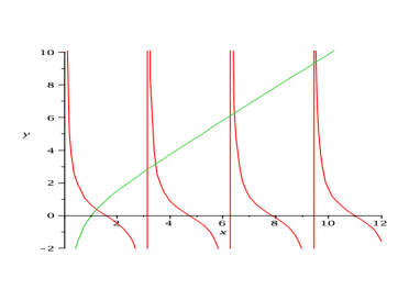
Figure 1: Solutions of Eq. (34), with $y=\cot(x)$ and $x=\pi\Omega\delta/g$, for cavities satisfying the condition $\delta\ll 1$. The asymptotes of the cotangent curve correspond to the frequencies of the field modes $\omega_{k}$.

Then, defining the dimensionless parameter

$$\delta=\frac{g}{\Delta\omega}=\frac{gR}{\pi c},$$ (33)

we rewrite Eq. (12) in the form

$$\cot\left(\frac{\pi\Omega\delta}{g}\right)=\frac{\Omega}{\pi g}+\frac{g}{\pi\delta\Omega}\left(1-\frac{\delta\bar{\omega}^{2}}{g^{2}}\right).$$ (34)

Taking $\delta\ll 1$, which corresponds to $R\ll\pi c/g$ (a small cavity), we find that, for $k=1,2,\ldots$, the solutions are

$$\Omega_{k}\approx\frac{g}{\delta}\left(k+\frac{2\delta}{\pi k}\right).$$ (35)

If we further assume that $\Omega_{0}\pi\delta/g\ll 1$, a condition compatible with $\delta\ll 1$, then $\Omega_{0}$ is found to be

$$\Omega_{0}\approx\bar{\omega}\left(1-\frac{\pi\delta}{3}\right).$$ (36)

To determine $f_{00}(t)$, we have to calculate the square of the matrix elements $\left(t_{0}^{0}\right)^{2}$ and $\left(t_{k}^{0}\right)^{2}$. They are given, to first order in $\delta$, by

$$\left(t_{0}^{0}\right)^{2}\approx\left(1+\frac{2\pi\delta}{3}\right)^{-1};\qquad\left(t_{k}^{0}\right)^{2}\approx\frac{4}{k^{2}}\frac{\delta}{\pi}(t_{0}^{0})^{2}.$$ (37)

We thus obtain, for sufficiently small cavities ($\delta\ll 1$),

$$\left|f_{00}(t)\right|^{2} \approx \left(1+\frac{2}{3}\pi\delta\right)^{-2}\left\{1+\frac{8\delta}{\pi}\sum_{k=1}^{\infty}\frac{1}{k^{2}}\cos\left[\bar{\omega}\left(1-\frac{\pi\delta}{3}\right)-\frac{g}{\delta}\left(k+\frac{2\delta}{\pi k}\right)\right]t\right.$$ (38)

$$+\left.\frac{16\delta^{2}}{\pi^{2}}\sum_{k,l=1}^{\infty}\frac{1}{k^{2}l^{2}}\cos\left[\left(\frac{g}{\delta}-\frac{2g}{\pi kl}\right)(k-l)\right]t\right\}.$$

To order $\delta^{2}$, a lower bound for $\left|f_{00}(t)\right|^{2}$ is obtained by taking the value $-1$ for both cosines in the above formula, using the tabulated value of the Riemann zeta function $\zeta(2)=\pi^{2}/6$:

$$\left|f_{00}(t)\right|^{2}\gtrsim\left(1+\frac{2}{3}\pi\delta\right)^{-2}\left\{1-\frac{4\pi\delta}{3}-\frac{4\pi^{2}\delta^{2}}{9}\right\}.$$ (39)

We see, comparing Eqs. (38) and (32) that the quantity $\left|f_{00}(t)\right|^{2}$, which dictates the behavior of the density matrix elements and of the measure of purity in Eq. (27), has very different behaviors for free space or for a small cavity. This implies that in the situation of a small cavity, in contrast to the free space case, all matrix elements in Eqs. (23) are different from $zero$ at all times.

In Fig. (2) the degree of impurity from Eq. (27) is plotted as a function of time in the cases of an arbitrarily large cavity ($R\rightarrow\infty$) and of a small cavity. We take $\delta=0.1$, with $\bar{\omega}=1.0$ and $g=0.5$ fixed (in arbitrary units).

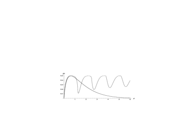
Figure 2: Behavior of the degree of impurity $D$ as function of time, equation (27), for a small cavity (dashed line) and a very large cavity (solid line); we take the parameters $g=0.5$, $\delta=0.1$ and $\bar{\omega}=1.0$ (in arbitrary units).

We see from the figure that for a very large cavity (free space) the two-atom system dissipates; with the passing of time, both atoms go to their ground states, only the element $\rho_{0_{\mathcal{A}}0_{\mathcal{B}}}^{0_{\mathcal{A}}0_{\mathcal{B}}}(t)=1$ survives in this limit. On the other hand, for a small cavity, the system never completely decays.

III.3 Time evolution of the von Neumann entropy

We now turn our attention to the von Neumann entropy associated with the reduced density matrix with respect to one of the subsystems; it is obtained by taking the trace over the states of the complementary subsystem in the full density matrix. For pure states of bipartite systems, it measures the degree of entanglement.

The reduced density matrix for the $t=0$ superposition of states in Eq. (LABEL:definition-entangled-state), $\rho_{\mathcal{A}}$, is obtained by tracing over the dressed $B$ atom. For $t\neq 0$, we have

$$\rho_{\mathcal{A}}(t) = \mathrm{Tr}_{\mathcal{B}}\left(\left|\Psi(t)\right\rangle\left\langle\Psi(t)\right|\right)$$ (40)

$$= \sum_{\mu,\nu}\xi f_{A\mu}(t)f_{A\nu}^{*}(t)\left|\Gamma_{100\cdots}^{\mu(A)}\right\rangle\left\langle\Gamma_{100\cdots}^{\nu(A)}\right|$$

$$+\,n(1-\xi)\left|\Gamma_{000\cdots}^{A}\right\rangle\left\langle\Gamma_{000\cdots}^{A}\right|.$$

As time goes on, we have the time-dependent von Neumann entropy given by

$$E(t,\xi) = -\mathrm{Tr}\left[\rho_{\mathcal{A}}(t)\ln\rho_{\mathcal{A}}(t)\right]$$ (41)

$$= -\sum_{\alpha}\alpha(t)\ln\alpha(t),$$

where here $\alpha(t)$ are the time-dependent eigenvalues of the reduced density matrix. These should be solutions of the characteristic equation, which in the case of (40), reads

$$\det\left(\begin{array}[]{ccccc}1-\xi-\alpha&0&0&0&\cdots\\ 0&\xi\left|f_{AA}\right|^{2}-\alpha&\xi f_{A1}f_{AA}^{*}&\xi f_{A2}f_{AA}^{*}&\cdots\\ 0&\xi f_{AA}f_{A1}^{*}&\xi\left|f_{A1}\right|^{2}-\alpha&\xi f_{A2}f_{A1}^{*}&\cdots\\ 0&\xi f_{AA}f_{A2}^{*}&\xi f_{A1}f_{A2}^{*}&\xi\left|f_{A2}\right|^{2}-\alpha&\cdots\\ \vdots&\vdots&\vdots&\vdots&\ddots\end{array}\right)=0.$$ (42)

We thus find that the only nonzero eigenvalues of $\rho_{\mathcal{A}}$ are

$$\alpha_{1}=1-\xi,\qquad\alpha_{2}=\xi\sum_{\mu}\left|f_{A\mu}(t)\right|^{2}=\xi,$$ (43)

which are time independent. This then implies that the von Neumann entropy takes the expression

$$E(t,\xi)=-\left[(1-\xi)\ln(1-\xi)+\xi\ln\left(\xi\right)\right],$$ (44)

which coincides with the von Neumann entropy associated with the initial state $\left|\Psi(0)\right\rangle$ given by Eq. (LABEL:definition-entangled-state); that is, all the time dependence of the von Neumann entropy for this two-atom system, coming from the quantities $f_{\lambda\nu}(t)$, is completely cancelled in the computation of the entropy, in all situations, with the maximum entanglement occuring at $\xi=1/2$. In other words, although the superposition of states evolves in time, in very different ways in the limits of a very large cavity and of a small one, the entangled nature of these two-atom states remains unchanged for all times, independently of the size of the cavity.

IV Concluding remarks

In this paper we have considered a system composed of two atoms in a spherical cavity, each of them in independent interaction with an environment field. The model employed is of a bipartite system, in which each subsystem consists of one of the atoms dressed by its own proper field. We make the assumption that initially we have a superposition of two states: one in which one of the dressed atoms is in its first excited level and the other atom and the field modes are all in the ground state; this state is superposed with another one in which the atoms have their roles reversed.

The time evolution of the superposition of these atomic states leads to a time-dependent (reduced) density matrix. Expressions for its elements are provided in both the cases of an infinitely large cavity (that is, free space) and of a small one, when the two atoms are considered as identical. Very different behaviors are obtained for this time evolution. In the large-cavity case, the system shows dissipation, and, with the passing of time, both atoms go to their ground states. For a small cavity, an oscillating behavior is present, so that the atoms never fully decay.

In spite of these rather contrasting behaviors and of the nontrivial time dependence of the density matrix, we obtain a von Neumann entropy which is independent of time and of the cavity size. We find that the initial entanglement of the two atoms remains unchanged as the system evolves, for a cavity of any size, in the approximation of noninteracting dressed atoms. This could be related to the fact that for multipartite systems the superposition principle leads naturally to entangled states; in this case noninteracting subsystems can thus share entangled states that hold quantum correlations. Such quantum entanglement carries nonlocal features which can be analyzed by comparison with classical correlations bel1 ; bel2 . If an interaction between the dressed atoms, mediated by their dressing clouds, is introduced, we expect that the von Neumann entropy associated to the dressed atoms can depend on time and on the size of the cavity. However, to establish the formalism of dressed coordinates and dressed states for a system of two interacting dressed atoms is a very hard task, which is perhaps not possible on purely analytical grounds. We can think of introducing this interaction as a kind of “perturbation” around the individually dressed atomic states. This will be the subject of future work.

We would like to emphasize that we here consider entanglement as a pure quantum effect, a characteristic of quantum mechanics, which is also nonlocal, in the sense that distant and non-interacting systems may be entangled. This is due to the existence of superposed states, not to the interaction between the (in our case, dressed) atoms. Indeed such properties of entanglement of non interacting systems have been used to conceive quantum communication devices bennet .

Noninteracting systems have been, and currently are, the subject of intense investigation in the realm of teleportation and quantum information theory. In lebedev , entanglement in a mesoscopic structure consisting of noninteracting parts is investigated. These authors study the time-dependent electron–electron and electron–hole correlations in a mesoscopic device and analyze the appearance of entanglement by means of a Bell inequality test and of Bell inequality tests based on coincidence probabilities. As we have already mentioned before, in the framework of the theory of quantum computating, a situation conceptually near to the one we investigate here is studied dajka : two noninteracting qubits, initially prepared in an entangled state, are coupled to their own independent environments and evolve under their influence. These authors find conditions for nonvanishing entanglement at arbitrary time, for both zero and nonzero temperatures. Also, in Ref. chan , a study of the entanglement evolution of two remote atoms interacting independently with a cavity field is presented. In sowa , quantum entanglement is approached for an ensemble of noninteracting electrons. This author uses this as a standpoint to study the interacting gas and claims that in this context the quantum Hall effect can be thought of as a basis for quantum computation.

The study of entangled states of noninteracting systems is interesting in itself. As clearly exposed in haffner , entanglement can exist as a purely quantum phenomenon among noninteracting particles, which are however described by the same wavefunction. Entanglement means that individual particles are not independent of each other, even if they do not interact, and their quantum properties are inextricably “tied up”, this being the origin of the Schrödinger’s original denomination, verschränkte Zustände, for these states. In this context, the influence of an atom on the other one is not due to an interaction between them, but is due to the attribution of physical meaning to superposed states, a concept with no correspondence in classical physics.

Acknowledgments: The authors acknowledge CNPq/MCT (Brazil) for partial financial support. APCM thanks FAPERJ (Brazil) for partial financial support.

References

- (1) W.G. Unruh and W.H. Zurek, Phys. Rev. D 40, 1071 (1989).
- (2) B.L. Hu, J.P. Paz and Y. Zhang, Phys. Rev. D 45, 2843 (1992).
- (3) H. Morawitz, Phys. Rev. A 7, 1148 (1973).
- (4) P. Milonni and P. Knight, Opt. Comm. 9, 119 (1973).
- (5) D. Kleppner, Phys. Rev. Lett. 47, 233 (1981).
- (6) G. Flores-Hidalgo, A.P.C. Malbouisson and Y.W. Milla, Phys. Rev. A 65, 063414 (2002).
- (7) A.P.C. Malbouisson, Ann. Phys. 308, 373 (2003).
- (8) G. Flores-Hidalgo and A.P.C. Malbouisson, Phys. Rev. A 66, 042118 (2002).
- (9) G. Flores-Hidalgo and A.P.C. Malbouisson, Phys. Lett. A 337, 37 (2005).
- (10) G. Flores-Hidalgo, C.A. Linhares, A.P.C. Malbouisson and J.M.C. Malbouisson, J. Phys. A 41, 075404 (2008).
- (11) N.P. Andion, A.P.C. Malbouisson and A. Mattos Neto, J. Phys. A 34, 3735 (2001); A.P.C. Malbouisson, Report Instituto Balseiro/CAB Bariloche, CAB/1971/13 (1971) (unpublished).
- (12) W. Jhe, A. Anderson, E.A. Hinds, D. Meschede, L. Moi and S. Haroche, Phys. Rev. Lett. 58, 666 (1987).
- (13) R.G. Hulet, E.S. Hilfer and D. Kleppner, Phys. Rev. Lett. 55, 2137 (1985).
- (14) P. Ullersma, Physica 32, 56; 74; 90 (1966).
- (15) F. Haake and R. Reibold, Phys. Rev. A 32, 2462 (1982).
- (16) A.O. Caldeira and A.J. Leggett, Ann. Phys. 149, 374 (1983).
- (17) H. Grabert, P. Schramm and G.-L. Ingold, Phys. Rep. 168, 115 (1988).
- (18) C. Cohen-Tannoudji, Atoms in Electromagnetic Fields (World Scientific, Singapore, 1994).
- (19) T. Petrosky, G. Ordonez and I. Prigogine, Phys. Rev. A 68, 022107 (2003).
- (20) F.C. Khanna, A.P.C. Malbouisson, J.M.C. Malbouisson and A.E. Santana, Thermal Quantum Field Theory: Algebraic Aspects and Applications (World Scientific, Singapore, 2009), chapter 24.
- (21) W. Thirring and F. Schwabl, Ergeb. Exakt. Naturw. 36, 219 (1964).
- (22) S. Chan, M.D. Reid and Z. Ficek, J. Phys. B - At., Mol. and Opt. Phys. 42, 065507 (2009).
- (23) J.S. Bell, Physics 1, 195 (1965).
- (24) J.S. Bell, Speakable and Unspeakable in Quantum Mechanics (Cambridge Univ. Press, Cambridge, 1965).
- (25) C. Bennett and S. Wiesner, Phys. Rev. Lett. 69, 2881 (1992).
- (26) A.V. Lebedev, G.B. Lesovik and G. Blatter, Phys. Rev. B 71, 045306 (2005).
- (27) J. Dajka, M. Mierzejewski and J. Luczka, Phys. Rev A 77, 042316 (2008).
- (28) A. Sowa, Theor. Math. Phys. 159, 654 (2009).
- (29) H. Häffner et al., Nature 438, 643 (2005).