Microlocal Analysis of the
Geometric Separation Problem

Abstract

Image data are often composed of two or more geometrically distinct constituents; in galaxy catalogs, for instance, one sees a mixture of pointlike structures (galaxy superclusters) and curvelike structures (filaments). It would be ideal to process a single image and extract two geometrically ‘pure’ images, each one containing features from only one of the two geometric constituents. This seems to be a seriously underdetermined problem, but recent empirical work achieved highly persuasive separations.

We present a theoretical analysis showing that accurate geometric separation of point and curve singularities can be achieved by minimizing the $\ell_{1}$ norm of the representing coefficients in two geometrically complementary frames: wavelets and curvelets. Driving our analysis is a specific property of the ideal (but unachievable) representation where each content type is expanded in the frame best adapted to it. This ideal representation has the property that important coefficients are clustered geometrically in phase space, and that at fine scales, there is very little coherence between a cluster of elements in one frame expansion and individual elements in the complementary frame. We formally introduce notions of cluster coherence and clustered sparsity and use this machinery to show that the underdetermined systems of linear equations can be stably solved by $\ell_{1}$minimization; microlocal phase space helps organize the calculations that cluster coherence requires.

Key Words. $\ell_{1}$ minimization. Sparse Representation. Mutual Coherence. Cluster Coherence. Tight Frames. Curvelets, Shearlets, Radial Wavelets.

Acknowledgements. The authors would like to thank Inam ur Rahman, Apple Computer, for graphics help, and Emmanuel Candès, Michael Elad, and Jean-Luc Starck, for numerous discussions on related topics. The second author would like to thank the Statistics Department at Stanford and the Mathematics Department at Yale for hospitality and support during her visits. Thanks also to the Isaac Newton Institute of Mathematical Sciences in Cambridge, UK for an inspiring research environment which led to the completion of a significant part of this work. This work was partially supported by NSF DMS 05-05303 and DMS 01-40698 (FRG), and by Deutsche Forschungsgemeinschaft (DFG) Heisenberg fellowship KU 1446/8-1.

1 Introduction

Cosmological data analysts face tasks of geometric separation [39, 40]. Gravitation, acting over time, drives an initially quasi-uniform distribution of matter in 3D to concentrate near lower-dimensional structures: points, filaments, and sheets. It would be desirable to process single ‘maps’ of matter density and somehow extract three ‘pure’ maps containing just the points, just the filaments, and just the sheets around which matter is concentrating.

In seemingly unrelated fields, such as medical imaging and materials science, related questions arise frequently and naturally. For example, a technologist with a single confused image of an aggregate might wish to create two images, one containing just the fibrous and the other just the granular structures, respectively.

Such ‘desires’, when voiced by a working scientist or engineer, really amount to a request for existing information technology to be put to work here and now on data available today. No doubt there is a wide spectrum of image processing ‘hacks’ and ‘improvisations’ that might be useful, on a case-by-case basis. The mathematician’s interest would only be piqued when an intellectually coherent approach shows promise of success, especially if the reasons for success are subtle and instructive.

Recently, astronomer Jean-Luc Starck and collaborators have been empirically successful in numerical experiments with component separation; their approach used tools from modern harmonic analysis in a provocative way. They used two or more overcomplete frames, each one specially adapted to particular geometric structures, and were able to obtain separation despite the fact that the underlying system of equations is highly underdetermined. Here we analyze such approaches in a mathematical framework where we can show that success stems from an interplay between geometric properties of the objects to be separated, and the harmonic analysis for singularities of various geometric types. We eventually point to a much wider range of seemingly very different ‘imaging’ problems where our analysis techniques can provide insight.

1.1 Singularities and Sparsity

As a mathematical idealization of ‘image’, consider a Schwartz distribution $f$ with domain ${\bf R}^{2}$. The distribution $f$ will be given singularities with specified geometry: points and curves.

We plan to represent such an ‘image’ using tools of harmonic analysis; in particular, bases and frames. While many such representations are conceivable, we are interested here just in those bases or frames which can sparsely represent $f$ – i.e., can represent $f$ using relatively few large coefficients.

The type of basis which best sparsifies $f$ depends on the geometry of its singularities. If the singularities occur at a finite number of (variable) points, then wavelets give what is, roughly speaking, an optimally sparse representation – one with the fewest significantly nonzero coefficients. If the singularities occur at a finite number of smooth curves, then one of the recently studied directional multiscale representations (curvelets or shearlets) will do the best job of sparsification. (For careful quantitative discussions of sparsification see, e.g., [6] etc.).

In fact, real-world signals are, generally speaking, a mixture of content types and, correspondingly, a model where singularities are of only one geometric type is overly narrow. If $f$ is actually a nontrivial superposition ${\cal P}+{\cal C}$ where ${\cal P}$ has only point singularities and ${\cal C}$ has only curvilinear singularities, then two things happen:

• Neither wavelets alone nor curvelets alone will be very good for representing ${\cal P}+{\cal C}$. The sparsity either achieves alone is much less satisfactory than the ideal sparsity level – that which could be achieved by using wavelets for representing ${\cal P}$ and by curvelets in representing ${\cal C}$. (This ideal representation is purely notional; it assumes one can first perfectly separate the two objects and then separately analyze the separated layers.)

• In fact, no single basis or traditional linear representation is very good at sparsifying ${\cal P}+{\cal C}$ compared to the ideal representation.

This immediately suggests the need to use both systems to represent $f$ sparsely; however, since each system is itself complete (or even overcomplete) there is no obvious traditional way to do this.

In this paper, we consider the problem of developing sparse representations by combining both wavelets and curvelets and using a nonlinear representation based on $\ell_{1}$ minimization. The problem we solve is a continuum variant of a problem in image and signal processing with considerable practical interest, and extensive work for almost two decades. For references, see Subsection 1.6 below. That work, while suggestive and inspiring, concerns discretely indexed signal/image processing, obscuring the continuum elements of geometry and microlocal analysis which are essential to this paper.

1.2 A Geometric Separation Problem

Consider the following simple but clear model problem of geometric separation. Consider a ‘pointlike’ object ${\cal P}$ made of point singularities:

$${\cal P}=\sum_{i=1}^{P}|x-x_{i}|^{-3/2}.$$ (1.1)

This object is smooth away from the $P$ given points $(x_{i}:1\leq i\leq P)$. Consider as well a ‘curvelike’ object ${\cal C}$, a singularity along a closed curve $\tau:[0,1]\mapsto{\bf R}^{2}$:

$${\cal C}=\int\delta_{\tau(t)}(\cdot)dt,$$ (1.2)

where $\delta_{x}$ is the usual Dirac delta function located at $x$. The singularities underlying these two distributions are geometrically quite different, but the exponent $\-3/2$ is chosen so the energy distribution across scales is similar; if ${\cal A}_{r}$ denotes the annular region $r<|\xi|<2r$,

$$\int_{{\cal A}_{r}}|\hat{{\cal P}}|^{2}(\xi)\asymp r,\qquad\int_{{\cal A}_{r}}|\hat{{\cal C}}|^{2}(\xi)\asymp r,\qquad r\rightarrow\infty.$$ (1.3)

This choice makes the components comparable as we go to finer scales; the ratio of energies is more or less independent of scale. Separation is challenging at every scale.

Now assume that we observe the ‘Signal’

$$f={\cal P}+{\cal C},$$ (1.4)

however, the component distributions ${\cal P}$ and ${\cal C}$ are unknown to us.

Definition 1.1

The Geometric Separation Problem requires to recover ${\cal P}$ and ${\cal C}$ from knowledge only of $f$; here ${\cal P}$ and ${\cal C}$ are unknown to us, but obey (1.1), (1.2) and certain regularity conditions on the curve $\tau$.

As there are two unknowns (${\cal P}$ and ${\cal C}$) and only one observation ($f$), the problem seems improperly posed. We develop a principled, rational approach which provably solves the problem according to clearly stated standards.

1.3 Two Geometric Frames

We now focus on two overcomplete systems for representing the object $f$:

• Radial Wavelets – a tight frame with perfectly isotropic generating elements.

• Curvelets – a highly directional tight frame with increasingly anisotropic elements at fine scales.

We pick these because, as is well known, point singularities are coherent in the wavelet frame and curvilinear singularities are coherent in the curvelet frame. In Section 8.1 we discuss other system pairs. For readers not familiar with frame theory, we refer to [11], where terms like ‘tight frame’ – a Parseval-like property – are carefully discussed.

The point- and curvelike objects we defined in the previous subsection are real-valued distributions. Hence, for deriving sparse expansions of those, we will consider radial wavelets and curvelets consisting of real-valued functions. So only angles associated with radians $\theta\in[0,\pi)$ will be considered, which later on we will, as is customary, identify with ${\bf P}^{1}$, the real projective line.

We now construct the two selected tight frames as follows. Let $W(r)$ be an ‘appropriate’ window function, where in the following we assume that $W$ belongs to $C^{\infty}({\bf R})$ and is compactly supported on $[-2,-1/2]\cup[1/2,2]$ while being the Fourier transform of a wavelet. For instance, suitably scaled Lemariè-Meyer wavelets possess these properties. We define continuous radial wavelets at scale $a>0$ and spatial position $b\in{\bf R}^{2}$ by their Fourier transforms

$$\hat{\psi}_{a,b}(\xi)=a\cdot W(a|\xi|)\cdot\exp\{ib^{\prime}\xi\}.$$

The wavelet tight frame is then defined as a sampling of $b$ on a series of regular lattices $\{a_{j}{\bf Z}^{2}\}$, $j\geq j_{0}$, where $a_{j}=2^{-j}$, i.e., the radial wavelets at scale $j$ and spatial position $k=(k_{1},k_{2})^{\prime}$ are given by the Fourier transform

$$\hat{\psi}_{\lambda}(\xi)=2^{-j}\cdot W(|\xi|/2^{j})\cdot\exp\{ik^{\prime}\xi/2^{j}\},$$

where we let $\lambda=(j,k)$ index position and scale.

For the same window function $W$ and a ‘bump function’ $V$, we define continuous curvelets at scale $a>0$, orientation $\theta\in[0,\pi)$, and spatial position $b\in{\bf R}^{2}$ by their Fourier transforms

$$\hat{\gamma}_{a,b,\theta}(\xi)=a^{\frac{3}{4}}\cdot W(a|\xi|)V(a^{-1/2}(\omega-\theta))\cdot\exp\{ib^{\prime}\xi\}.$$

See [7] for more details. The curvelet tight frame is then (essentially) defined as a sampling of $b$ on a series of regular lattices

$$\{R_{\theta_{j,\ell}}D_{a_{j}}{\bf Z}^{2}\},\qquad j\geq j_{0},\quad\ell=0,\dots,2^{\lfloor j/2\rfloor}-1,$$ (1.5)

where $R_{\theta}$ is planar rotation by $\theta$ radians, $a_{j}=2^{-j}$, $\theta_{j,\ell}=\pi\ell/2^{j/2}$, $\ell=0,\dots,2^{j/2}-1$, and $D_{a}$ is anisotropic dilation by $diag(a,\sqrt{a})$, i.e., the curvelets at scale $j$, orientation $\ell$, and spatial position $k=(k_{1},k_{2})$ are given by the Fourier transform

$$\hat{\gamma}_{\eta}(\xi)=2^{-j\frac{3}{4}}\cdot W(|\xi|/2^{j})V((\omega-\theta_{j,\ell})2^{j/2})\cdot\exp\{i(R_{\theta_{j,\ell}}D_{2^{-j}}k)^{\prime}\xi\},$$

where let $\eta=(j,k,\ell)$ index scale, orientation, and scale. (For a precise statement, see [8, Section 4.3, pp. 210-211]).

Roughly speaking, the radial wavelets are ‘radial bumps’ with position $k/2^{j}$ and scale $2^{-j}$, while the curvelets live on anisotropic regions of width $2^{-j}$ and length $2^{-j/2}$. The wavelets are good at representing point singularities while the curvelets are good at representing curvilinear singularities.

Using the same window $W$, we can construct a family of filters $F_{j}$ with transfer functions

$$\hat{F}_{j}(\xi)=W(|\xi|/2^{j}),\qquad\xi\in{\bf R}^{2}.$$

These filters allow us to decompose a function $f$ into pieces $f_{j}$ with different scales, the piece $f_{j}$ at subband $j$ arises from filtering $f$ using $F_{j}$:

$$f_{j}=F_{j}\star f;$$

the Fourier transform $\hat{f}_{j}$ is supported in the annulus with inner radius $2^{j-1}$ and outer radius $2^{j+1}$. Because of our assumption on $W$, we can reconstruct the original function from these pieces using the formula

$$f=\sum_{j}F_{j}\star f_{j},\qquad f\in L^{2}({\bf R}^{2}).$$

The tight frames of curvelets and radial wavelets discussed above interact in a very local way with the filtering $F_{j}$.

Lemma. Let ${\cal F}_{j}$ denote the range of the operator of convolution with $F_{j}$. Then curvelets at level $j^{\prime}$ are orthogonal to ${\cal F}_{j}$ unless $|j^{\prime}-j|\leq 1$. Similarly, radial wavelets at level $j^{\prime}$ are orthogonal to ${\cal F}_{j}$ unless $|j^{\prime}-j|\leq 1$.

Proof. Indeed, ${\cal F}_{j}$ is the collection of all functions $f_{j}$ whose Fourier transform is representable as $\hat{f}_{j}(\xi)=W(|\xi|/2^{j})\hat{f}(\xi)$ where $f\in L^{2}({\bf R}^{2})$. The support in frequency space of elements of ${\cal F}_{j}$ is thus an annulus ${\cal A}_{j}$ (say). The annuli have disjoint interiors if $|j-j^{\prime}|>1$. Hence ${\cal F}_{j}\perp{\cal F}_{j^{\prime}}$ if $|j^{\prime}-j|>1$.

However, both the radial wavelet frame elements and the curvelet frame elements at level $j^{\prime}$ belong to ${\cal F}_{j^{\prime}}$. $\Box$

For future use, let $\Lambda_{j}$ denote the collection of indices $(j,k)$ of wavelets at level $j$, and

$$\Lambda_{j}^{\pm n}=\bigcup_{j^{\prime}=j-n}^{j+n}\Lambda_{j^{\prime}}.$$

Similarly, let $\Delta_{j}$ denote the indices $\eta=(j,k,\ell)$ of curvelets at level $j$, and let

$$\Delta_{j}^{\pm n}=\bigcup_{j^{\prime}=j-n}^{j+n}\Delta_{j^{\prime}}.$$

We conclude that elements of ${\cal F}_{j}$ can be represented using either only radial wavelets $\{\psi_{\lambda}:\lambda\in\Lambda_{j}^{\pm 1}\}$ or only curvelets $\{\gamma_{\eta}:\eta\in\Delta_{j}^{\pm 1}\}$.

1.4 Separation via $\ell_{1}$ Minimization

1.4.1 Sparse Multiple Frame Expansions

We now have two complete representations for ${\cal F}_{j}$, yielding two ways of representing the subband component $f_{j}$: in terms of its wavelet expansion:

$$f_{j}=\sum_{\lambda\in\Lambda_{j}^{\pm 1}}w_{\lambda}\psi_{\lambda};$$

or in terms of its curvelet expansion:

$$f_{j}=\sum_{\eta\in\Delta_{j}^{\pm 1}}c_{\eta}\gamma_{\eta}.$$

Each frame exhibits a single geometric tendency – either highly nondirectional or highly directional – in representing $f_{j}$. However, $f_{j}$ may have both isotropic and directional features. We therefore seek a combined representation

$$f_{j}=\sum_{\lambda\in\Lambda_{j}^{\pm 1}}w_{\lambda}\psi_{\lambda}+\sum_{\eta\in\Delta_{j}^{\pm 1}}c_{\eta}\gamma_{\eta}.$$

Because the combined frame formed by concatenating the two frames is overcomplete, there are many possible ways this decomposition can be done. Some of them may be geometrically motivated, many are not.

Consider the following dual-frame Component Separation problem based on $\ell_{1}$ minimization:

$$(\mbox{\sc CSep})\qquad(W_{j},C_{j}) = \mbox{ argmin }\|w\|_{1}+\|c\|_{1}$$

$$\quad\mbox{subject to }f_{j}=W_{j}+C_{j}$$

$$\qquad\mbox{ and }w_{\lambda}=\langle W_{j},\psi_{\lambda}\rangle,\quad\lambda\in\Lambda_{j}^{\pm 1}$$

$$\qquad\mbox{ and }c_{\eta}=\langle C_{j},\gamma_{\eta}\rangle,\quad\eta\in\Delta_{j}^{\pm 1}.$$

In words, we take a given scale subband $f_{j}$ and decompose it into a wavelet component $W_{j}$ and a curvelet component $C_{j}$. The components are chosen by the principle of $\ell_{1}$ minimization on the frame coefficients: the $\ell_{1}$ norm of the wavelet coefficients of the wavelet component should be small, and the $\ell_{1}$ norm of the curvelet coefficients of the curvelet component should be small.

Here is our reason for the ‘component separation’ label: Armed with the optimization result at each scale subband, we define the purported pointlike component as the superposition of all the wavelet terms:

$$\tilde{P}=\sum_{j}F_{j}\star W_{j};$$

and the purported curvelike component as the superposition of all the curvelet terms:

$$\tilde{C}=\sum_{j}F_{j}\star C_{j}.$$

We obtain the decomposition

$$f=\tilde{P}+\tilde{C}.$$

1.4.2 Main Result

At this stage, we have two decompositions: one by the truly geometric pair $({\cal P},{\cal C})$ of pointlike and curvelike objects and one by the purported geometric pair $(\tilde{P},\tilde{C})$. The following result justifies our interest in the second pair. To state it, define the scale subbands of the truly geometric components by:

$${\cal P}_{j}=F_{j}\star{\cal P};\qquad{\cal C}_{j}=F_{j}\star{\cal C}.$$

Theorem 1.1

Asymptotic Separation.

$$\frac{\|W_{j}-{\cal P}_{j}\|_{2}+\|C_{j}-{\cal C}_{j}\|_{2}}{\|{\cal P}_{j}\|_{2}+\|{\cal C}_{j}\|_{2}}\rightarrow 0,\qquad j\rightarrow\infty.$$ (1.6)

At fine scales, the truly pointlike component is almost all captured by the wavelet component and the truly curvelike component is almost all captured by the curvelet component. In short, the purported pointlike and curvelike components deserve the labelling they have been given.

1.5 Extensions

Theorem 1.1 is amenable to generalizations and extensions. Previewing Section 8.1, we mention a few examples.

• More General Classes of Objects. Theorem 1.1 can be generalized to other situations. First, we could consider singularities of different orders. This would allow ${\cal C}$ to model ‘cartoon’ images, where the curvilinear singularities are now the boundaries of the pieces for piecewise $C^{2}$ functions. Second, we can allow smooth perurbations, i.e., $f=({\cal P}+{\cal C}+g)\cdot h$ where $g,h$ are smooth functions of rapid decay at $\infty$. In this situation, we let the denominator in (1.6) be simply $\|f_{j}\|_{2}$.

• Other Frame Pairs. Theorem 1.1 holds without change for many other pairs of frames and bases, such as, e.g., orthonormal separable Meyer wavelets and shearlets.

• Noisy Data. Theorem 1.1 is resilient to noise impact; an image composed of ${\cal P}$ and ${\cal C}$ with additive ‘sufficiently small’ noise exhibits the same asymptotic separation.

• Rate of Convergence. Theorem 1.1 can be accompanied by explicit decay estimates.

• Other Algorithms and Other Notions of Separation. In the companion paper [20] we study thresholding as an alternative approach to separation; it is less computationally demanding than the $\ell^{1}$ minimization studied here, but also somewhat less elegant. Building on the estimates proved in this paper, [20] shows that properly-tuned thresholding can also achieve asymptotic separation.

1.6 The Multiple-Basis Representation Problem

Theorem 1.1 should be placed in context of a great deal of ongoing work concerning sparsity and overcomplete representations. Already in the early 1990’s, R.R. Coifman became interested in the problem of representing discrete-time signals using more than one basis. In a conversation, he told one of us about a problem which, in retrospect and using modern formulations, can be posed as follows:

• An observed signal $S\in{\bf R}^{n}$ is thought to be a superposition of subsignals $S_{i}$, $i=1,2$.

• Each subsignal $S_{i}$ is thought to be ‘coherent’ in an ‘appropriate’ basis $\Phi_{i}$, $i=1,2$.

• Each subsignal ’looks incoherent’ in an ‘inappropriate’ basis. Here $\Phi_{2}$ is inappropriate for $S_{1}$, and $\Phi_{1}$ is inappropriate for $S_{2}$.

Coifman, Wickerhauser and co-workers at the time made a sort of heuristic exploration motivated intuitively by these slogans. As a published example of their work at the time, please see [12, Fig. 26(a-h)]. The different ‘coherent parts’ displayed in those figures were obtained by the following recipe:

1. Transform signal $S$ into basis $\Phi_{1}$.

2. Threshold the coefficients, yielding sparse coefficients $\tilde{\alpha}_{1}$.

3. Form residual $R=S-\Phi_{1}\tilde{\alpha}_{1}$.

4. Transform $R$ into basis $\Phi_{2}$.

5. Threshold the coefficients, yielding sparse coefficients $\tilde{\alpha}_{2}$.

6. Write $\tilde{S}_{i}=\Phi_{i}\tilde{\alpha}_{i}$; then

   $$S=\tilde{S}_{1}+\tilde{S}_{2}+residual.$$ (1.7)

At about the same time, Stéphane Mallat and Zhifeng Zhang became interested in the problem of representing signals using a highly overcomplete dictionary of time-frequency atoms; [34] (their dictionary had $\approx\log(N)$ different frames, where $N$ is the signal length). Their approach, called Matching Pursuit, built up an approximation one-term-at-a-time iteratively, at each stage finding the best single atom in any of the several bases which was not yet already forming part of the approximation and adding that term to the approximation.

Lurking in these early numerical experiments were two larger questions. If there truly is a simple representation of the signal using more than one system, can it ever be found? Can it be found by such a simple approach?

Formally: can one accurately recover ‘coherent’ pieces $S_{1}$ and $S_{2}$ given knowledge of $S=S_{1}+S_{2}$ only? For example, can we expect that the outputs $\tilde{S}_{1}$, $\tilde{S}_{2}$ in (1.7) obey $\tilde{S}_{1}\approx S_{1}$ and $\tilde{S}_{2}\approx S_{2}$? Researchers at the time said in conversation, that, when put this starkly, the answer was simply ‘no’, since there are twice as many unknowns as knowns. Nevertheless, some of the empirical results at the time were suggestive and inspiring.

1.7 Minimum $\ell_{1}$ Decomposition and Perfect Separation

A few years later, one of us worked with Scott Shaobing Chen to develop a formal, optimization-based approach to the multiple-basis representation problem. Given bases $\Phi_{i}$, $i=1,2$, one solves the following problem

$$(\mbox{\sc BP})\qquad\min\|\alpha_{1}\|_{1}+\|\alpha_{2}\|_{1}\mbox{ subject to }S=\Phi_{1}\alpha_{1}+\Phi_{2}\alpha_{2}.$$

Here $\|\cdot\|_{1}$ denotes the usual $\ell_{1}$ norm. Note that here there are $2n$ unknowns in $\alpha_{1}$ and $\alpha_{2}$ and only $n$ knowns in $S$, but that an optimization principle is being used to select a particular element from the $n$-dimensional space of all possible solutions. (Terminological note: the name ’Basis Pursuit’ is meant to remind the reader that (BP) actually selects a basis for the solution out of the many conceivable bases which can be extracted from the union of the two overcomplete systems).

Based on earlier experience of our first-named author and his collaborators, see [19, 22, 23], it was known that the $\ell_{1}$ norm had a tendency to find sparse solutions when they exist. And indeed, Chen’s thesis showed that in some simple special cases that this was so. Letting $\Phi_{1}$ be the standard basis of ${\bf R}^{n}$ (i.e., Kronecker sequences or ‘spikes’) and $\Phi_{2}$ be the Fourier basis, Chen considered signals $S$ which were superpositions of two spikes and two sinusoids. He showed that (BP) recovered exactly the indices and coefficients of the terms involved in the synthesis; and that this was true across a wide range of amplitude ratios between the sinusoid and spike components. In short, there was perfect separation of sinusoids from spikes, and the true underlying simplicity of the signal was revealed – even though there were more unknowns than equations.

In the years since that work, two streams of research emerged.

• Theoretical work, showing that, indeed, one could in certain settings obtain the sparsest possible representations to an underdetermined problem by $\ell_{1}$ optimization; see, e.g., [9, 13, 14, 15, 17, 45] for a selection of general work concerning $\ell_{1}$ minimization, and [2, 16, 18, 24, 27] for work somewhat relevant to component separation.

• Empirical work, showing that combined representations such as wavelets with curvelets or wavelets with sinusoids often gave very compelling separations of real signals and images, see, for instance, [1, 10, 25, 26, 35, 42, 40, 41, 43, 44, 30, 47].

We have already mentioned the empirical successes of Starck and collaborators. For an overview of much recent work on sparse decompositions, see [3]. Note that geometric separation is somewhat different from the task of separation of texture from smooth structure; in that problem, sparsity in frame expansions does not play an explicit role, nor do the geometric considerations which are so important here; very interesting early work in such non-geometric separation was published by Yves Meyer [36], and Vese and Osher [37].

1.8 Theorem 1.1 in Context, and Outline of Paper

We can now place our result in context, via several comparisons and contrasts, looking ahead to themes developed below.

• Microlocal Viewpoint. In Theorem 1.1 the objects of interest are collections of point and curve singularities. The viewpoint derives from microlocal analysis (see Section 3), which says that points and curves are very different objects in their joint space/orientation structure, so that even if they happen to overlap spatially, they are microlocally distinct. In contrast, other work on sparsity and $\ell_{1}$ minimization typically has a discrete flavor, making hypotheses about the number of nonzeros in an expansion and assuming the dictionary elements interact randomly.

• Microlocal Asymptotics. Asymptotics are important for Theorem 1.1; the sharp separation between curves and points in microlocal phase space exists only as a limit phenomenon, as the scale tends to zero. Asymptotic statements are important in other literature on sparsity-driven decompositions, but they are asymptotic in the number of random elements in the underlying matrix, and exploit law-of-large-numbers and concentration-of-measure effects. For Theorem 1.1, such principles play no role.

• Clustered Sparsity. In other work on sparsity-driven decompositions, sparsity of the coefficients plays a role primarily through the number of nonzeros. In this work sparsity plays a role also through the arrangement of nonzeros; Section 2.1 introduces a notion of clustered sparsity and Sections 4-7 develop estimates bounding the locations of significant nonzeros in the wavelet expansion of a point singularity or in the curvelet expansion of a curve singularity; the estimates will be organized using micolocal phase space ideas described in Section 3.

• Cluster Coherence. In other work on sparsity-driven decompositions, coherence or restricted isometry principles play a role; these don’t depend on the arrangement of nonzeros in an expansion. Moreover, these are often applied to random-dictionary situations where the interaction between frame elements is random and quasi arbitrary. Section 2.1 develops the notion of cluster coherence which specifically depends on the arrangement of nonzeros. We apply this notion to a dictionary (wavelets + curvelets) where interactions are geometrically driven, and we develop estimates motivated by microlocal analysis which provide the needed geometrical information.

Our paper begins with Sections 2 and 3 introducing the driving ideas of clustered sparsity, cluster coherence, and microlocal separation, and describing a plan to prove Theorem 1.1 by establishing several needed estimates. Later Sections 4, 5, 6, and 7 then develop these estimates, by developing results about wavelet and curvelet expansions of point and line singularities. Section 8 then mentions a number of possible extensions.

2 Component Separation by $\ell_{1}$ Minimization

We now study the behavior of $\ell^{1}$ minimization in the two-frame case. Our analysis centers on the use of cluster coherence to control joint concentration.

2.1 $\ell_{1}$ Minimization for Separation of Two Tight Frames

Suppose we have two tight frames $\Phi_{1}$, $\Phi_{2}$ in a Hilbert space ${\cal H}$, and a signal vector $S\in{\cal H}$. We know a priori that there exists a decomposition

$$S=S_{1}^{0}+S_{2}^{0},$$

where $S_{1}^{0}$ is sparse in Frame 1, and $S_{2}^{0}$ is sparsely represented in Frame 2.

Consider the following optimization problem

$$(\mbox{Sep})\qquad(S_{1}^{\star},{S}_{2}^{\star})=\mbox{argmin}_{S_{1},S_{2}}\|\Phi_{1}^{T}S_{1}\|_{1}+\|\Phi_{2}^{T}S_{2}\|_{1}\mbox{ subject to }S=S_{1}+S_{2}.$$ (2.1)

The optimization problem $(\mbox{\sc Sep})$ is visibly similar to, but subtly different from, $(\mbox{\sc BP})$. Here the $\ell_{1}$ norm is being applied on the analysis coefficients of the two different ‘components’ rather than on the individual synthesis coefficients. The hope in $(\mbox{\sc BP})$ is to get exactly the right nonzero coefficients in the sense of those providing the sparsest representation. However, this can become numerically unstable for certain tight frames. The hope in $(\mbox{\sc Sep})$ is merely to separate components rather than the more ambitious goal of identifying the true nonzero coefficients within each component’s representation. Starck and Elad have found this distinction to be important in their own empirical work on separation.

To analyze this we need the following notion.

Definition 2.1

Let $\Phi_{1}$ and $\Phi_{2}$ be two tight frames. Given two sets of coefficients ${\cal S}_{1}$ and ${\cal S}_{2}$, define the joint concentration $\kappa=\kappa({\cal S}_{1},{\cal S}_{2})$ by

$$\kappa({\cal S}_{1},{\cal S}_{2})=\sup_{f}\frac{\|1_{{\cal S}_{1}}\Phi_{1}^{T}f\|_{1}+\|1_{{\cal S}_{2}}\Phi_{2}^{T}f\|_{1}}{\|\Phi_{1}^{T}f\|_{1}+\|\Phi_{2}^{T}f\|_{1}}.$$

In words, we consider the maximal fraction of total $\ell_{1}$ norm which can be concentrated to the combined index set ${\cal S}_{1}\cup{\cal S}_{2}$. Concepts of this kind go back to [23]. Adequate control of joint concentration ensures that the principle (2.1) gives a successful approximate separation.

Proposition 2.1

Suppose that $S$ can be decomposed as $S=S_{1}^{0}+S_{2}^{0}$ so that each component $S_{i}^{0}$ is relatively sparse in $\Phi_{i}$, $i=1,2$, i.e.,

$$\|1_{{\cal S}_{1}^{c}}\Phi_{1}^{T}S_{1}^{0}\|_{1}+\|1_{{\cal S}_{2}^{c}}\Phi_{2}^{T}S_{2}^{0}\|_{1}\leq\delta.$$

Let $(S_{1}^{\star},S_{2}^{\star})$ solve (2.1). Then

$$\|S_{1}^{\star}-S_{1}^{0}\|_{2}+\|S_{2}^{\star}-S_{2}^{0}\|_{2}\leq\frac{2\delta}{1-2\kappa}.$$

Definition 2.2

Given tight frames $\Phi=(\phi_{i})_{i}$ and $\Psi=(\psi_{j})_{j}$ and an index subset ${\cal S}$ associated with expansions in frame $\Phi$, we define the cluster coherence

$$\mu_{c}({\cal S},\Phi;\Psi)=\max_{j}\sum_{i\in{\cal S}}|\langle\phi_{i},\psi_{j}\rangle|.$$

In many studies of $\ell_{1}$ optimization, one utilizes instead the mutual coherence

$$\mu(\Phi,\Psi)=\max_{j}\max_{i}|\langle\phi_{i},\psi_{j}\rangle|,$$ (2.2)

whose importance was shown by [18]. This may be called the singleton coherence. In contrast, cluster coherence bounds coherence between a single member of frame $\Psi$ and a cluster of members of frame $\Phi$, clustered at ${\cal S}$.

A related notion called ‘cumulative coherence’ was introduced in [45]; that notion maximizes over subsets ${\cal S}$ of a given size, whereas here we fix a specific set ${\cal S}$ of coefficients. In applying our concept, the index subsets we will consider are not abstract, but will instead have a specific geometric interpretation, associated to proximity to certain curves in phase space. Maximizing over all subsets of a given size would give very loose bounds, and would not be suitable for our purposes. Several other coherence measures involving subsets appear in the literature, e.g., [4] and [46], but we do not see a strong relation to cluster coherence.

Lemma 2.1

We have

$$\kappa({\cal S}_{1},{\cal S}_{2})\leq\max\{\mu_{c}({\cal S}_{1},\Phi_{1};\Phi_{2}),\mu_{c}({\cal S}_{2},\Phi_{2};\Phi_{1})\}.$$

The proofs for Proposition 2.1 and Lemma 2.1 are presented in Section 9.1.

2.2 Intended Application

The concepts of this section will now be applied to (CSep), at scale $j$ only. With $f={\cal P}+{\cal C}$ our distribution of interest, and $F_{j}$ our bandpass filter, and we set $f_{j}=F_{j}\star f$. Throughout this section, the object $S\equiv f_{j}$ and the tight frames are $\Phi_{1}$, the full radial wavelet frame, and $\Phi_{2}$, the full curvelet tight frame. We apply the optimization problem (Sep), getting subsignal components $S_{1}^{\star}$ and $S_{2}^{\star}$, which we then relabel as the wavelet component $W_{j}$ and curvelet component $C_{j}$; one should check that with this sequence of substitutions, problem (Sep) of this section becomes (CSep) of the introduction.

The key problem in the application of Proposition 2.1 to the aforementioned setting is the correct choice of the clusters of significant coefficients at each scale. If those clusters are chosen ‘too small asymptotically’, the relative sparsity will blow up, and if chosen ‘too large asymptotically’, we lose control of the cluster coherence. We define those clusters on the ideal decomposition, where wavelets are used to analyze the point singularity and curvelets are used to analyze the curve singularity. (Such clusters are theoretical, non-observable entities.)

For a series of wavelet-coefficient thresholds ${\varepsilon}_{j,1}$ to be specified, the cluster of significant wavelet coefficients can be provisionally defined as

$${\cal S}_{1,j}=\{\lambda\in\Lambda_{j}^{\pm 1}:|\langle\psi_{\lambda},{\cal P}_{j}\rangle|>{\varepsilon}_{j,1}\cdot\|(\langle\psi_{\lambda^{\prime}},{\cal P}_{j}\rangle)_{\lambda^{\prime}}\|_{\ell_{\infty}(\Lambda_{j}^{\pm 1})}\}.$$ (2.3)

For a series of curvelet-coefficient thresholds ${\varepsilon}_{j,2}$ to be specified, the cluster of significant curvelet coefficients can be provisionally taken as

$${\cal S}_{2,j}=\{\eta\in\Delta_{j}^{\pm 1}:|\langle\gamma_{\eta},{\cal C}_{j}\rangle|>{\varepsilon}_{j,2}\cdot\|(\langle\gamma_{\eta^{\prime}},{\cal C}_{j}\rangle)_{\eta^{\prime}}\|_{\ell_{\infty}(\Delta_{j}^{\pm 1})}\}.$$ (2.4)

Each threshold choice picks a specific point on the tradeoff between relative sparsity and cluster coherence.

Then $\delta_{j}$ will denote the degree of approximation by significant coefficients, the sum $\delta_{j}=\delta_{j,1}+\delta_{j,2}$ of the wavelet approximation error to the point singularity:

$$\delta_{j,1}=\sum_{\lambda\in{\cal S}_{1,j}^{c}}|\langle\psi_{\lambda},{\cal P}_{j}\rangle|;$$

and the curvelet approximation error to the curvilinear singularity:

$$\delta_{j,2}=\sum_{\eta\in{\cal S}_{2,j}^{c}}|\langle\gamma_{\eta},{\cal C}_{j}\rangle|.$$

Finally, $\kappa({\cal S}_{1,j},{\cal S}_{2,j})$, the degree of joint wavelet-curvelet concentration at the significant subsets, will be controlled by two cluster coherences: $\mu_{c}({\cal S}_{1,j},\Phi_{1};\Phi_{2})$ the maximal coherence of a curvelet to a cluster of significant wavelet coefficients; and $\mu_{c}({\cal S}_{2,j},\Phi_{2};\Phi_{1})$ the maximal coherence of a wavelet to a cluster of significant curvelet coefficients. We have

Corollary 2.1

Suppose that the sequence of transform-space clusters $({\cal S}_{1,j})$, and $({\cal S}_{2,j})$ has both of the following two properties: (i) asymptotically negligible cluster coherences:

$$\mu_{c}({\cal S}_{1,j},\Phi_{1};\Phi_{2}),\mu_{c}({\cal S}_{2,j},\Phi_{2};\Phi_{1})\rightarrow 0,\qquad j\rightarrow\infty,$$

and (ii) asymptotically negligible cluster approximation errors:

$$\delta_{j}=\delta_{1,j}+\delta_{2,j}=o(\|f_{j}\|_{2}),\qquad j\rightarrow\infty.$$

Then we have asymptotically near-perfect separation:

$$\frac{\|W_{j}-{\cal P}_{j}\|_{2}+\|C_{j}-{\cal C}_{j}\|_{2}}{\|f_{j}\|_{2}}\rightarrow 0,\qquad j\rightarrow\infty.$$

The main result –Theorem 1.1 – follows from this lemma, but this will require sufficiently good estimates for cluster coherence for clusters defined as sufficiently good approximations to the objects of interest.

We remark that although the threshold in the provisional definition of the clusters in (2.3)-(2.4) provides a means to balance between relative sparsity and cluster coherence, there is no a priori guarantee that there exists a threshold for which conditions (i) and (ii) of Corollary 2.1 are true. The main achievement of this paper is to show that this is indeed possible with a revised definition. In fact we do not finally define the clusters by (2.3)-(2.4); note that the clusters must simply exhibit properties (i) and (ii) of the Corollary. We intend to make use of our freedom of definition in order to get the needed properties.

3 Microlocal Analysis Viewpoint

The proof of the main result boils down to defining clusters and bounding cluster coherences and cluster approximation errors; our approach is inspired by microlocal analysis. In effect, we consider the case where the cluster is either a string of curvelet coefficients in the cone of influence of a curvilinear singularity, or a block of wavelet coefficients in the cone of influence of a point singularity, and we must bound interactions between clusters in one frame and elements in the other frame. Microlocal analysis provides a simple organizational framework that immediately suggests which interactions ’ought’ to be small and large, based on the geometry of the overlaps between phase portraits in the underlying microlocal phase space.

3.1 Microlocal Analysis Concepts

The singular support of a distribution $f$, $\mbox{sing supp}(f)$, is the set of points where $f$ is not locally $C^{\infty}$. In the geometric separation setting, we have

$$\mbox{sing supp}(f)=\mbox{sing supp}({\cal P}+{\cal C})=\mbox{sing supp}({\cal P})\cup\mbox{sing supp}({\cal C})=\{x_{i}\}\cup image(\tau)$$

because we have constructed the distributions ${\cal P}$ and ${\cal C}$ so their singularities have this form.

Note that the points $x_{i}$ can intersect the image of the curve $\tau$ – we make no separation hypothesis asking the point singularities to ‘stay away’ from the curvilinear singularities. Figure 1 displays the singular support of $f$ and the contributions from ${\cal P}$ and ${\cal C}$.

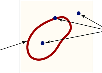
Figure 1: Singular supports of the point singularity ${\cal P}$ and the curvilinear singularity ${\cal C}$. The two supports overlap in one point.

To properly separate between pointlike and curvelike singularities we need to consider a phase space for microlocal analysis indexed by position-orientation pairs $(b,\theta)$; such pairs can describe the locations and orientations where $f$ has singular behavior. The orientational component $\theta$ will be regarded as an element in ${\bf P}^{1}$, the real projective space in ${\bf R}^{2}$. (Here we identify ${\bf P}^{1}$ with $[0,\pi)$ and freely write one or the other in what follows. It may at first seem more natural to think of directions $[0,2\pi)$ rather than orientations $[0,\pi)$, note however that in this paper we consider real-valued distributions ${\cal P}+{\cal C}$ measured by real-valued curvelets $\gamma_{\eta}$ so directions are not resolvable, only orientations. We also frequently abuse notation as follows: we will write $|\theta-\theta^{\prime}|$ when what is actually meant is geodesic distance between two points on ${\bf P}^{1}$.)

Living in this phase space is the wavefront set $WF(f)$; roughly, this is the set of position-orientation pairs at which $f$ is nonsmooth; for more details, see: [29, 7, 31].

Under the geometric separation model of Section 1, we have

$$WF({\cal P})=\mbox{supp}({\cal P})\times{\bf P}^{1},$$

since a point singularity is singular in all directions on its singular support, and is singular nowhere else; while

$$WF({\cal C})=\{(\tau(t),\theta(t)):t\in[0,L(\tau)]\}$$

where $\tau(t)$ is a unit-speed parametrization of ${\cal C}$ and $\theta(t)$ is the normal direction to ${\cal C}$ at $\tau(t)$ regarded in ${\bf P}^{1}$.

It is convenient to think of the parameter space for microlocal analysis as a plane ${\bf R}^{2}$ of positions $b$ lying beneath a third dimension of orientations $\theta$. Then the wavefront set of a point singularity ${\cal P}$ concentrated on a single point $x_{1}$ is a vertical line segment $\{x_{1}\}\times{\bf P}^{1}$, corresponding to singular behavior in every direction at a given point, while the wavefront set of ${\cal C}$ is a more general curve in phase space. Even if $x_{1}$ meets $image(\tau)$, so the singular support of the point singularity and a curvilinear singularity overlap at $x_{1}$, they behave quite differently as wavefront sets in the full 3D parameter space, which gives us hope for separation.

Figure 2 illustrates the 3D phase space with pointlike and curvelike singularities superposed.

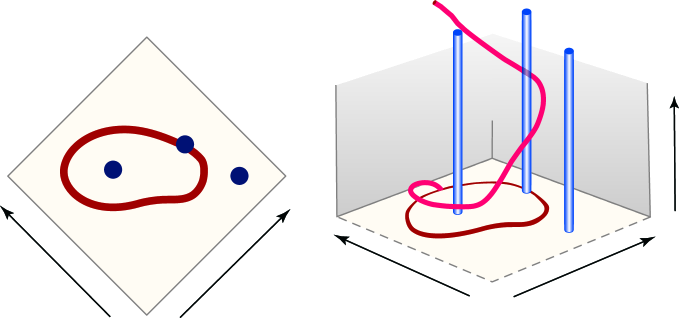
Figure 2: Left panel: singular supports of ${\cal P}$ and ${\cal C}$ (compare Figure 1). Right panel: wavefront sets of ${\cal P}$ and ${\cal C}$ are indicated by blue and red tubes in $(b_{1},b_{2},\theta)$ space. The singular support of ${\cal C}$ is also indicated; it is the $b_{1}$-$b_{2}$ projection of the wavefront set. Due to the additional dimension, the wavefront sets are more distinctly separated than the corresponding singular supports.

3.2 Support of Frame Elements

A radial wavelet $\psi_{\lambda}$, $\lambda=(a_{0},b_{0})$ is ‘morally’ supported in $x$-space in a spatial ball $B(a_{0},b_{0})$, defined by

$$B(a_{0},b_{0})=\{x:|x-b_{0}|/a\leq 1\};$$

this statement should not however be taken too literally, as the radial wavelets we study are not of compact support. The more precise statement is that the wavelet decays rapidly in the variable $|x-b_{0}|/a$. The next statement uses the notation

$$\langle a\rangle=(1+a^{2})^{1/2}.$$

Lemma 3.1

For each $N=1,2,\dots$ there is a constant $c_{N}$ so that

$$|\psi_{a,b}(x)|\leq c_{N}\cdot a^{-1}\cdot\langle|x-b|/a\rangle^{-N},\qquad\forall a\in{\bf R}^{+}\;\forall b,x\in{\bf R}^{2}.$$

An individual curvelet $\gamma_{\eta}$, $\eta=(a_{0},b_{0},\theta_{0})$ is ‘morally’ supported in $x$-space inside an anisotropic spatial ellipse. To make this precise, let $D_{1/a}$ be the diagonal matrix $diag(1/a,1/\sqrt{a})$ and $R_{-\theta}$ denote planar rotation by $-\theta$ radians. Let

$$P_{a,\theta}=D_{1/a}R_{-\theta}$$

denote the parabolic directional dilation operator which dilates much more strongly in the $\theta$ direction than in the orthogonal direction. For a vector $v\in{\bf R}^{2}$ define the norm

$$|v|_{a,\theta}=|P_{a,\theta}(v)|;$$

the unit ball in this norm is ellipsoidal, with minor axis pointing in direction $\theta$. A curvelet is morally supported in the ellipse $E(a_{0},b_{0},\theta_{0})$ defined by

$$E(a_{0},b_{0},\theta_{0})=\{x:|x-b_{0}|_{a_{0},\theta_{0}}\leq 1\},$$

Again the correct formal statement is that there is rapid decay in the variable $|x-b|_{a,\theta}$. The following is proved in [7, Lemma 1, page 168].

Lemma 3.2

For each $N=1,2,\dots$ there is a constant $c_{N}$ so that

$$|\gamma_{a,b,\theta}(x)|\leq c_{N}\cdot a^{-3/4}\cdot\langle|x-b|_{a,\theta}\rangle^{-N},\qquad\forall a\in{\bf R}^{+}\;\forall\theta\in[0,\pi)\;\forall b,x\in{\bf R}^{2}.$$ (3.1)

In Figure 3, we visualize these support relationships.

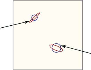
Figure 3: Effective supports of wavelets and curvelets at different scales. The shapes of those supports become increasingly distinct with increasingly fine scales.

3.3 Phase-Space Support of Frame Elements

We also study the location-orientation behavior of frame elements, i.e., the attribution of regions in an orientation/location domain as regions of significant activity in a distribution $f$. The wavefront set gives a qualitative way to do this; we use the continuous curvelet transform (CCT) to do so quantitatively. This transform is defined by

$$\Gamma_{f}(a,b,\theta)=\langle\gamma_{a,b,\theta},f\rangle$$

and is indexed by triples $(a,b,\theta)$, where $a>0$, $b\in{\bf R}^{2}$, and $\theta\in[0,\pi)$; this associates a function $f$ to a scale/location/direction domain. There is a natural measure on this domain:

$$m(da,db,d\theta)=a^{-3}\cdot da\cdot db\cdot d\theta.$$

Consider a high-pass function $f$, i.e., one whose Fourier transform of $f$ vanishes near the origin; $\hat{f}(\xi)=0$, $|\xi|\leq\pi/a_{0}$, see [7]. The CCT offers a Parseval relationship for high-pass functions:

$$\int\int\int|\Gamma_{f}(a,b,\theta)|^{2}m(da,db,d\theta)=\|f\|_{2}^{2},$$

see [8]. Hence the energy in $f$ is distributed through the scale-location-direction domain by the curvelet transform offering a portrait of the function’s significant activity.

Consider the transform of a radial wavelet:

$$\Gamma_{\psi_{a_{0},b_{0}}}(a,b,\theta)=\langle\gamma_{a,b,\theta},\psi_{a_{0},b_{0}}\rangle,\qquad a>0,\;b\in{\bf R}^{2},\;\theta\in[0,\pi).$$

Because $\psi_{a_{0},b_{0}}$ is radial, $\Gamma_{\psi_{a_{0},b_{0}}}(a,b,\theta)$ is constant, independent of $\theta$, and decays rapidly in variables $|\log_{2}(a/a_{0})|$ and $|b-b_{0}|/a_{0}$. It is morally localized to a cell of the form

$$W(a_{0},b_{0})=\{(a,b,\theta):|\log_{2}(a/a_{0})|<1,\theta\in[0,\pi),|b-b_{0}|/a_{0}\leq 1\};$$

we have the following formal statement, proved in Subsection 9.2.1 below:

Lemma 3.3

For each $N=1,2,\dots$, there is a constant $c_{N}$ so that

$$|\langle\gamma_{a,b,\theta},\psi_{a_{0},b_{0}}\rangle|\leq c_{N}\cdot a^{1/4}\cdot 1_{\{|\log_{2}(a/a_{0})|<3\}}\cdot\langle|b-b_{0}|_{a,\theta}\rangle^{-N}.$$

It implies the following for a scale-conditional phase portrait of a wavelet (i.e., we freeze the analysis scale $a$ at a specific value, and inspect $\Gamma_{\psi_{a_{0},b_{0}}}(a,b,\theta)$ as a function of variables $b$ and $\theta$): when freezing $a=a_{0}$, we see that $\Gamma$ is ‘morally’ supported in a vertical tube above the point $b_{0}$; each horizontal cross-section is a ball of width $a_{0}$, i.e., $B(a_{0},b_{0})$.

Consider now the transform of a curvelet:

$$\Gamma_{\gamma_{a_{0},b_{0},\theta_{0}}}(a,b,\theta)=\langle\gamma_{a,b,\theta},\gamma_{a_{0},b_{0},\theta_{0}}\rangle,\qquad a>0,\;b\in{\bf R}^{2},\;\theta\in[0,\pi).$$

This is ‘morally’ localized to a cell of the following form:

$$Q(a_{0},b_{0},\theta_{0})=\{(a,b,\theta):|\log_{2}(a/a_{0})|<1,|\theta-\theta_{0}|<\sqrt{a_{0}},|b-b_{0}|_{a_{0},\theta_{0}}\leq 1\};$$

the correct formal statement being [see (21) in [8]]

Lemma 3.4

For each $N=1,2,\dots$, there is a constant $c_{N}$ so that

$$|\langle\gamma_{a,b,\theta},\gamma_{a_{0},b_{0},\theta_{0}}\rangle|\leq c_{N}\cdot 1_{\{|\log_{2}(a/a_{0})|<3\}}\cdot 1_{\{|\theta-\theta_{0}|<10\sqrt{a_{0}}\}}\cdot\langle|b-b_{0}|_{a_{0},\theta_{0}}\rangle^{-N}.$$

(We remind the reader of our convention that, for two points $\theta,\theta^{\prime}\in[0,\pi)$, $|\theta-\theta^{\prime}|$ really means geodesic distance in ${\bf P}^{1}$.)

Thus each curvelet is supported in scale, location, direction in a set which effectively has a product structure, and is compactly supported in both scale and orientation. In a scale-conditional phase portrait, freezing $a=a_{0}$, we see a vaguely ellipsoidal structure with slice $\theta=\theta_{0}$ exhibiting an anisotropic footprint, like $E(a_{0},b_{0},\theta_{0})$.

In Figure 4 we visualize the scale-conditional portraits of a wavelet and a curvelet.

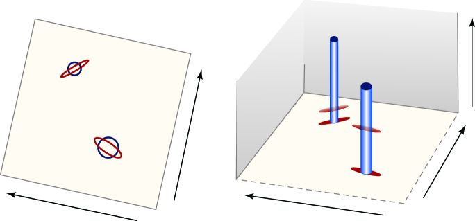
Figure 4: Left panel: effective supports of wavelets (blue) and curvelets (red); compare Figure 3. Right Panel: Phase space portrait – obtained by CCT – of the same wavelets and curvelets. Effective supports of curvelets are indicated in the $(b_{1},b_{2})$ plane. The portrait conveys the intuition that while the effective support of wavelets and curvelets may overlap substantially in the spatial domain, in the full phase space, the relative overlap is significantly reduced.

The intuition to be fostered from these figures is that curvelets don’t interact very heavily with wavelets, because they have such different support in $(b,\theta)$, even when they have the same scale and location parameters, $a_{0}$ and $b_{0}$.

This support structure of curvelets is notable for other reasons. The support structure is implicit in the natural measure:

$$m(da,db,d\theta) = a^{-3}\cdot da\cdot db\cdot d\theta$$

$$= \quad\frac{da}{a}\cdot\frac{db}{a^{3/2}}\cdot\frac{d\theta}{a^{1/2}},\qquad 0<a<a_{0},b\in{\bf R}^{2},\;\theta\in{\bf P}^{1}.$$

The second expression has the following interpretation. We assign roughly unit measure to curvelet cells

$$m(Q(a,b,\theta))\approx 1,\qquad 0<a<a_{0},\;b\in{\bf R}^{2},\theta\in{\bf P}^{1};$$

there are about $a^{-3/2}$ locations per unit volume at a fixed scale and orientation and about $a^{-1/2}$ orientations at a fixed scale and location.

The support structure is mimicked by the discretization of the curvelet tight frame, which morally breaks the $(a,b,\theta)$ domain into disjoint cells $Q(a_{j},b_{j,k,\ell},\theta_{j,\ell})$ and samples the continuous transform once per cell; for details see [8].

3.4 CCT of Singularities

The CCT can be used to analyze the singularities ${\cal P}$ and ${\cal C}$ directly. Let’s impose regularity conditions on ${\cal C}$.

Let the Hausdorff pseudo-distance $d$ between $b$ and a curve $\tau$ be defined by

$$d(a,b,\theta;\tau)=\min\{|x-b|_{a,\theta}:x\in image(\tau)\}.$$

Definition 3.1

A finite-length planar curve $\tau$ will be called parabolically regular, if, for $N=1,2,\dots$, there is a constant $c_{N}$ so that for $a\in(0,1)$ and all $b,\theta$,

$$\int\langle|\tau(t)-b|_{a,\theta}\rangle^{-N}dt\leq c_{N}\cdot a^{1/2}\cdot\langle d(a,b,\theta;\tau)\rangle^{-N}.$$ (3.2)

Traditional nice curves, such as line segments, circles, etc. are parabolically regular, though we skip the demonstration.

Lemma 3.5

Let the singularity ${\cal C}$ be defined as in (1.2) by a parabolically regular curve $\tau$. Then, for each $N=1,2,\dots$,

$$|\Gamma_{{\cal C}}(a,b,\theta)|\leq c_{N}\cdot a^{-1/4}\cdot\langle d((a,b,\theta);\tau)\rangle^{-N}.$$

In words, the CCT may be large at phase space points close to $\tau$, but elsewhere it is very small.

Proof. The definition of ${\cal C}$ as a linear functional on the Schwartz space gives

$$\Gamma_{{\cal C}}(a,b,\theta)=\int\gamma_{a,b,\theta}(\tau(t))dt.$$

The estimates (3.1) and (3.2) give

$$|\Gamma_{{\cal C}}(a,b,\theta)| \leq \int c_{N}\cdot a^{-3/4}\cdot\langle|\tau(t)-b|_{a,\theta}\rangle^{-N}dt$$

$$\leq c_{N}\cdot a^{-3/4}\cdot C^{\prime}_{N}\cdot a^{1/2}\cdot\langle d(a,b,\theta;\tau)\rangle^{-N}$$

$$= C^{\prime\prime}_{N}\cdot a^{-1/4}\cdot\langle d(a,b,\theta;\tau)\rangle^{-N}.\mbox{$\Box$}$$

3.5 Heuristics

We are now in a position to give a heuristic explanation why the strategy announced in Section 2.2 is likely to work. In effect, there are very instructive analogies between the calculations needed to implement that strategy and the behavior of certain ‘tubes’ in phase space. The reader will have noticed that the curvelet parameter $(a,b,\theta)$ and the wavefront set parameter $(b,\theta)$ differ only by the latter’s provision of a scale. Hence there is some analogy between the scale-conditional portrait by CCT and the wavefront set – both provide measures of the activity of an object, indexed by location and orientation.

In effect, the scale-conditional portrait by CCT is a “thickened-out” version of the wavefront set. A point singularity has a wavefront set which is a vertical line in phase space, and a scale-conditional portrait which is localized near a thin vertical tube. A curvilinear singularity has a wavefront set which is a curve in phase space, while Lemma 3.5 says that, morally, the curvelet transform of the object ${\cal C}$ ‘lives’ near a tube. The tube in question has thickness $\approx a$. Look at the scale-conditional portrait, and define the tube

$$T(a_{0})=\bigcup_{b,\theta}(E(a_{0},b,\theta)\times\{\theta\}),$$

where the union is over $b$, $\theta$ satisfying

$$d((a_{0},b,\theta);\tau)\leq 1.$$

As $a_{0}\rightarrow 0$, this tube shrinks down to a curve $\tilde{\tau}$ in phase space ${\bf R}^{2}\times{\bf P}^{1}$ defined by

$$\tilde{\tau}(t)=(\tau(t),\theta(t)),$$

where $\theta(t)$ is the orientation of the normal to $\tau(t)$. In short, in the sense of set convergence

$$T(a_{0})\rightarrow WF({\cal C}),\qquad a_{0}\rightarrow 0.$$

Thus, the wavefront set and the curvelet transform both signal that the activity in location-orientation space is concentrated near $image(\tilde{\tau})$.

More is true. A wavelet has a scale-conditional portrait which is a thin vertical tube – similar to the phase portrait of a point singularity – while a curvelet has a scale-conditional portrait which is a tube surrounding a little ‘piece of a curve’ in phase space, i.e., it morally has a position and orientation.

This visual analogy suggests that curvelets are incoherent to wavelets – because of the low overlap in phase space. Indeed, from Parseval,

$$\int\int\int\Gamma^{\star}_{\psi_{a_{0},b_{0}}}(a,b,\theta)\Gamma_{\gamma_{a_{1},b_{1},\theta_{1}}}(a,b,\theta)m(da,db,d\theta)=\langle\psi_{a_{0},b_{0}},\gamma_{a_{1},b_{1},\theta_{1}}\rangle,$$

and so the low overlap between the two phase portraits indeed will cause relatively low singleton coherence (2.2); indeed the tubelet associated to a given curvelet and the tube associated to a given wavelet visibly have relatively small overlap in the scale-conditional phase portrait; for example, if we compare the overlap of effective supports in phase space to the overlap of effective supports in the spatial domain, we see that the fractional overlap is dramatically smaller at fine scales in the phase space portrait than it is in the spatial domain portrait.

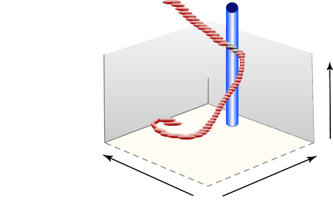
Figure 5: Phase space portrait of a cluster of curvelets and one single wavelet. Note the visually small overlap of these two geometrical objects. This suggests by analogy that each single wavelet is not coherent with anything built from such a cluster of curvelets.

However, the singleton coherence is not sufficiently small to be powerful in the present setting. Instead, this paper develops cluster coherence. The visual analogy presented in Figure 5 suggests how to bound the cluster coherence and suggests that the proof strategy of Section 2.2 will succeed. To understand that analogy, let’s study Figure 5. If we let ${\cal S}_{1}$ denote the set of significant wavelet coefficients in the radial wavelet transform of ${\cal P}$ at scale $a_{0}$, and ${\cal S}_{2}$ denote the set of significant curvelet coefficients in the curvelet transform of ${\cal C}$ at scale $a_{0}$, we believe the reader will be easily able to motivate the following assertions on the basis of Figures 3-5:

• Wavelets in ${\cal S}_{1}$ are associated to vertical tubes clustering around the point singularities in ${\cal P}$;

• Curvelets in ${\cal S}_{2}$ are associated with tubes clustering around the curvilinear phase portrait of ${\cal C}$;

• No single wavelet’s phase portrait overlaps much with the cluster of curvelet phase portraits of ${\cal S}_{2}$;

• No single curvelet phase portrait overlaps with the cluster of wavelets in ${\cal S}_{1}$.

Let’s outline a pseudo-calculation inspired by these visual observations. First, we consider a pseudo-calculation of the cluster coherence,

$$\mu_{c}({\cal S}_{1,j},\mbox{\sc Wavelet scale $j$};\mbox{\sc Curvelet scale $j$})=\sup_{\eta}\sum_{\lambda\in{\cal S}_{1,j}}|\langle\gamma_{\eta},\psi_{\lambda}\rangle|.$$

With $(\psi_{i})_{i}$ an enumeration of the significant wavelets in the expansion at scale $a_{j}=2^{-j}$,

$$\sum_{i}|\langle\gamma_{\eta},\psi_{i}\rangle| = \sum_{i}\left|\int\int\int\Gamma_{\gamma_{\eta}}^{*}\Gamma_{\psi_{i}}dm\right|$$

$$\leq \sum_{i}\int\int\int|\Gamma_{\gamma_{\eta}}|(a,b,\theta)|\Gamma_{\psi_{i}}|(a,b,\theta)dm$$

$$\leq \int\int\int|\Gamma_{\gamma_{\eta}}|(a,b,\theta)\sum_{i}|\Gamma_{\psi_{i}}|(a,b,\theta)dm.$$

Now use the bounds on $|\Gamma_{\psi_{i}}|(a,b,\theta)$ given above in Lemma 3.3, and deploy the slogan that only a bounded number of significant wavelets at any given scale interact strongly with any specific phase space point; we have

$$\sum_{i}|\Gamma_{\psi_{i}}|(a,b,\theta)\lesssim C_{1}\cdot a_{j}^{1/4},$$

where the sum is over the significant wavelets at scale $a_{j}$ and $C_{1}$ does not depend on $j$, and the symbol $\lesssim$ indicates an inequality motivated heuristically – in this case by the preceding italicized slogan. We also observe that Lemma 3.4 implies that the integral over phase space of a curvelet phase portrait obeys $\int\int\int|\Gamma_{\gamma_{\eta}}|(a,b,\theta)dm\leq C_{2}$. Combining this with the previous displays, we pseudo-conclude that

$$\mu_{c}({\cal S}_{1},\mbox{\sc Wavelet scale $j$};\mbox{\sc Curvelet scale $j$})\rightarrow 0,\qquad j\rightarrow\infty.$$

Next, we consider a pseudo-calculation of the cluster coherence

$$\mu_{c}({\cal S}_{2},\mbox{\sc Curvelet scale $j$};\mbox{\sc Wavelet scale $j$})=\sup_{\lambda}\sum_{\eta\in{\cal S}_{2,j}}|\langle\gamma_{i},\psi_{\lambda}\rangle|.$$

With $(\gamma_{i})_{i}$ an enumeration of the significant curvelets in the expansion at scale $a_{j}=2^{-j}$, then for a fixed wavelet index $\lambda$ we have

$$\sum_{i}|\langle\gamma_{i},\psi_{\lambda}\rangle| = \sum_{i}\left|\int\int\int\Gamma_{\gamma_{i}}^{*}\Gamma_{\psi_{\lambda}}dm\right|$$

$$\leq \sum_{i}\int\int\int|\Gamma_{\gamma_{i}}|(a,b,\theta)|\Gamma_{\psi_{\lambda}}|(a,b,\theta)dm$$

$$\leq \int\int\int|\Gamma_{\psi_{\lambda}}|(a,b,\theta)\sum_{i}|\Gamma_{\gamma_{i}}|(a,b,\theta)dm.$$

Now use the bounds on $|\Gamma_{\gamma_{i}}|(a,b,\theta)$ given above in Lemma 3.4, and apply the slogan that only a bounded number of significant curvelets at any given scale interact strongly with a given phase space point. We have

$$\sum_{i}|\Gamma_{\gamma_{i}}|(a,b,\theta)\lesssim C_{1},$$

where the sum is over the significant curvelets at scale $a_{j}$ and $C_{1}$ is a constant. We also observe that Lemma 3.3 implies that the integral over phase space of a wavelet phase portrait obeys $\int\int\int|\Gamma_{\psi_{\lambda}}|(a,b,\theta)dm\leq C_{2}\cdot a_{0}^{1/4}$, where $a_{0}=a_{0}(\lambda)$. Combining this with the previous displays, we pseudo-conclude that

$$\mu_{c}({\cal S}_{2},\mbox{\sc Curvelet scale $j$};\mbox{\sc Wavelet scale $j$})\rightarrow 0,\qquad j\rightarrow\infty.$$

We now turn to the approximation tasks posed by the strategy announced in Section 2.2. To pseudo-bound $\delta_{j,1}$, we fix ${\varepsilon}>0$ and define the tube in phase space ${\cal T}_{j,1}$ consisting of all scale/location pairs $(a,b)$ where the bound provided in Lemma 4.1 permits coefficients larger than $a_{j}^{1-{\varepsilon}}$. Also, we let $i_{j}$ denote the index in the wavelet enumeration beyond which such potentially significant coefficients can no longer arise. We can heuristically approximate a sum of wavelet coefficients with an integral over the phase space region covered by the union of their phase space supports; then we have

$$\delta_{j,1} = \sum_{i>i_{j}}|\langle\psi_{i},{\cal P}_{j}\rangle|$$

$$\lesssim c_{N}\cdot a_{j}^{-1/2}\cdot\int\int\int_{{\cal T}_{j,1}^{c}}\langle b/a_{j}\rangle^{-N}dm.$$

For sufficiently large $N$, the integrand has powerful decay; for large $j$, the width of the tube ${\cal T}_{j,1}$ is significantly wider than the decay scale $a_{j}$; and so the integral becomes negligible for large $j$, i.e., we pseudo-conclude that $\delta_{j,1}\rightarrow 0$. To pseudo-bound $\delta_{j,2}$ we fix ${\varepsilon}>0$ and define the tube in phase space ${\cal T}_{j,2}$ consisting of all triples $(a,b,\theta)$ where the bound provided in Lemma 3.5 permits coefficients larger than $a_{j}^{1-{\varepsilon}}$. Also we let $i_{j}$ denote the index in the curvelet enumeration beyond which such potentially significant coefficients can no longer arise; again heuristically identifying a sum with a phase-space integral we have

$$\delta_{j,2} = \sum_{i>i_{j}}|\langle\gamma_{i},{\cal C}_{j}\rangle|$$

$$\lesssim c_{N}\cdot\int\int\int_{{\cal T}_{j,2}^{c}}a^{-1/4}\cdot\langle d(a_{j},b,\theta;\tau)\rangle^{-N}dm.$$

For large $N$ the integrand decays strongly; for large $j$ the width of the tube is significantly wider than the decay scale $a_{j}$; and so again the integral becomes negligible for large $j$, i.e., we pseudo-conclude that $\delta_{j,2}\rightarrow 0$.

In short, phase space diagrams, some elementary estimates motivated by tube overlaps, and some cardinality ‘slogans’ combine to show plausibility of the strategy announced in Section 2.2. In the sections to come, we rigorously carry out that strategy. While the details are much more delicate than this plausibility argument would suggest, the architecture of our full demonstration remains faithful to the geometric viewpoint.

4 The Cluster ${\cal S}_{1,j}$ and its estimates

In this section, we define the cluster of wavelet coefficients ${\cal S}_{1,j}$ of the filtered point singularity $F_{j}\star{\cal P}$, and estimate relative sparsity as well as cluster coherence using this cluster. We intend to show that with this definition of cluster set,

$$\delta_{1,j}=o(\|f_{j}\|_{2}),\qquad j\rightarrow\infty,$$ (4.1)

and

$$\mu_{c}({\cal S}_{1,j},\{\psi_{\lambda}\};\{\gamma_{\eta}\})\rightarrow 0,\qquad j\rightarrow\infty.$$ (4.2)

As explained in Section 2.2, this gives the needed part of Theorem 1.1 having to do with ${\cal S}_{1,j}$.

WLOG we can assume that

$${\cal P}=|x|^{-3/2}.$$

The result for the more general ${\cal P}$ of (1.1) follows easily by combining translation invariance with finitely many uses of the triangle inequality. We also, from now on, fix some

$${\varepsilon}\in(0,1/32).$$

Our first lemma is used frequently in what follows, and is crucial for our definition of the cluster of wavelet coefficients. For the proof, see Subsection 9.3.1.

Lemma 4.1

For each $N=1,2,\dots$, there is a constant $c_{N}$ so that

$$|\langle\psi_{a_{j^{\prime}},b},{\cal P}_{j}\rangle|\leq c_{N}\cdot 2^{j/2}\cdot 1_{\{|j-j^{\prime}|\leq 1\}}\cdot\langle|b/a_{j}|\rangle^{-N},\qquad\forall j,j^{\prime}\in{\bf Z}_{+},\;\forall b\in{\bf R}^{2}.$$

In line with the heuristics of the previous section, we think of our estimate as describing relative overlaps of tubes in phase space. However, in the particular case of wavelets, there is no directional selectivity, so all that matters is the projection of phase space onto the spatial domain. We measure spatial distances with

$$d_{2}(x,A)=\min_{a\in A}\|x-a\|_{2},\quad x\in{\bf R}^{2},\,A\subseteq{\bf R}^{2},$$

the Euclidean distance between a point $x$ and a set $A$.

Of course, since we are dealing with frames, ultimately we have to consider discrete indices. To support geometric intuition, most of our arguments will be in the continuum setting, restrictions to discrete sampling grids being delayed as late in each argument as possible.

Morally, the points in phase space associated with significant wavelet coefficients are contained in a tube around $WF({\cal P})$ in phase space. This neighborhood of $WF({\cal P})$ can be explicitly defined by

$${\mathcal{N}}_{1}^{PS}(a)=\{b\in{\bf R}^{2}:d_{2}(b,\{0\})\leq D_{1}(a)\}\times[0,\pi),$$

where

$$D_{1}(a)=a^{(1-{\varepsilon})}.$$

The shape of the tube reflects the isotropic behavior of $WF({\cal P})$. For an illustration of ${\mathcal{N}}_{1}^{PS}(a)$, we refer to Figure 6.

We define the cluster of wavelet coefficients around the point-singularity by intersecting the tube ${\mathcal{N}}_{1}^{PS}(a)$ with the wavelet lattice, i.e.,

$${\cal S}_{1,j}=\{(j,k)\in\Delta_{j}^{\pm 1}:\{b_{j,k}\}\times[0,\pi)\in{\mathcal{N}}_{1}^{PS}(a_{j})\}.$$

The remainder of the section establishes (4.1)-(4.2) for this definition of cluster.

4.1 Size of $f_{j}$

Lemma 4.2

For some $c>0$,

$$\|f_{j}\|_{2}\geq c2^{j/2},\qquad j\rightarrow\infty.$$

Proof. Apply (1.3) and (1.4):

$$\|f_{j}\|_{2}^{2} = \int_{{\bf R}^{2}}W^{2}(|\xi|/2^{j})|\hat{f}(\xi)|^{2}d\xi\geq c\cdot\int_{{\cal A}_{j}}|\xi|^{-1}d\xi\geq c\cdot 2^{j}.\qquad\mbox{$\Box$}$$

4.2 ${\cal S}_{1,j}$ offers low approximation error

Now we are ready to state and prove the approximation error of ${\cal S}_{1,j}$.

Lemma 4.3

$$\delta_{1,j}=\sum_{\lambda\in{\cal S}_{1,j}^{c}}|\langle\psi_{\lambda},{\cal P}_{j}\rangle|=o(\|f_{j}\|_{2}),\qquad j\rightarrow\infty.$$

Proof. Due to the specific filtering we use,

$$\delta_{1,j}=\sum_{\lambda\in{\cal S}_{1,j}^{c}}|\langle\psi_{\lambda},{\cal P}_{j}\rangle|=\sum_{j^{\prime}=j-1}^{j+1}\sum_{\{k:\{b_{j^{\prime},k}\}\times[0,\pi)\not\in{\mathcal{N}}_{1}^{PS}(a_{j^{\prime}})\}}|\langle\psi_{(j^{\prime},k)},{\cal P}_{j}\rangle|.$$

Applying Lemma 4.1, and picking $N$ so large that $(N-1){\varepsilon}>1/2$

$$\delta_{1,j}\leq c\cdot\sum_{|k|>2^{j{\varepsilon}}}c_{N}\cdot 2^{j/2}\cdot\langle|k|\rangle^{-N}=o(1),\qquad j>j_{0}.$$

So the lemma is proved. $\Box$

4.3 ${\cal S}_{1,j}$ offers low cluster coherence

Lemma 4.4

$$\mu_{c}({\cal S}_{1,j},\{\psi_{\lambda}\};\{\gamma_{\eta}\})\rightarrow 0,\qquad j\rightarrow\infty.$$

Proof. By Lemma 3.3, if $\lambda\in\Lambda_{j}^{\pm 1}$,

$$|\langle\psi_{\lambda},\gamma_{\eta}\rangle|\leq c\cdot 2^{-j/4},\qquad\forall\eta.$$

The definition of ${\cal S}_{1,j}$ via ${\mathcal{N}}_{1}^{PS}(a_{j})$ implies that

$$\#({\cal S}_{1,j})\leq c\cdot 2^{2j{\varepsilon}},\qquad\mbox{for sufficiently large }j.$$

We conclude from ${\varepsilon}<1/8$ that

$$\sup_{\eta}\sum_{\lambda\in{\cal S}_{1,j}}|\langle\psi_{\lambda},\gamma_{\eta}\rangle|\leq c\cdot 2^{-j(1/4-2{\varepsilon})}\rightarrow 0,\qquad j\rightarrow\infty.\qquad\mbox{$\Box$}$$

5 Sparse Expansion of a Linear Singularity

After the relative ease with which we obtained concentration estimates (4.1)-(4.2) for the cluster of significant wavelet coefficients, we must now brace ourselves for the considerably harder challenge posed by the analogous estimates for the cluster of significant curvelet coefficients. This extra work seems, at least to us, much more rewarding, as it involves a full-blown use of phase space geometry.

In this section, we develop essential infrastructure for the analysis to come, documenting the sparsity of curvelet coefficients of a special linear singularity. Let $w_{2}:{\bf R}\mapsto[0,1]$ be a smooth function to be specified later (cf. Subsection 6.2), supported in $[-1,1]$, and define the very special distribution $w{\cal L}$ supported on a line segment $\{0\}\times[-\rho,\rho]$ by

$$w{\cal L}=w_{2}(x_{2}/\rho)\cdot\delta_{0}(x_{1}).$$

Then we can write

$$\widehat{w{\cal L}}=\hat{w}\star\hat{{\cal L}},$$

where

$$\hat{w}=\hat{w}_{2}(\rho\xi_{2})\cdot\rho\cdot\delta_{0}(\xi_{1})\quad\mbox{and}\quad\hat{{\cal L}}=\delta_{0}(\xi_{2}).$$

Thus the action of $w{\cal L}$ on a continuous function $f$ is given by

$$2\pi\langle w{\cal L},f\rangle=\langle{\cal L},\hat{w}\star\hat{f}\rangle=\int(\hat{w}\star\hat{f})(\xi_{1},0)d\xi_{1}.$$ (5.1)

Conceptually, $w{\cal L}$ is a straight curve fragment; our analysis of ${\cal C}$ in Section 6 will reduce to the study of this case.

Define a tube in phase space, in which the significant curvelet coefficients will be located. This will now be a neighborhood of $WF(w{\cal L})$, defined by

$${\mathcal{N}}_{2}^{PS}(a)=\{b\in{\bf R}^{2}:d_{2}(b,\{0\}\times[-2\rho,2\rho])\leq D_{2}(a)\}\times[0,\sqrt{a}],$$

where

$$D_{2}(a)=a^{(1-{\varepsilon})}.$$

For an illustration of ${\mathcal{N}}_{2}^{PS}(a)$, and its relation to ${\mathcal{N}}_{1}^{PS}(a)$, we refer to Figure 6. The actual definition of the cluster of curvelet coefficients is much more involved. In Lemma 5.4, we will introduce a first set which helps to determine its location.

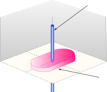
Figure 6: The tubes ${\mathcal{N}}_{1}^{PS}(a)$ and ${\mathcal{N}}_{2}^{PS}(a)$ in phase space. The clusters of significant coefficients correspond roughly to phase-space support regions overlapping these tubes.

Several bounds will control the curvelet coefficients of a linear singularity. Lemma 3.5 gives

$$|\langle w{\cal L},\gamma_{a,b,\theta}\rangle|\leq c\cdot 2^{j/4},\qquad\forall a,b,\theta;$$ (5.2)

in fact that lemma even gives a decay estimate, as the microlocation $(b,\theta)$ moves away from $(\{0\}\times[-\rho,\rho])\times\{0\}$. In the situations where we would use that decay estimate, the next lemma is more convenient.

Lemma 5.1

Suppose that $\theta\in[0,\sqrt{a}]$, and set

$$\tau:=\cos\theta\sin\theta(a^{-1}-a^{-2}),\quad d_{1}^{2}:=b_{1}^{2}(\sigma_{2}^{2}-\sigma_{1}^{-2}\tau),$$

and

$$d_{2}^{2}:=\left\{\begin{array}[]{ccl}\min_{\pm}\left((\pm\rho-b_{2})\sigma_{1}+\sigma_{1}^{-1}b_{1}\tau\right)^{2}&:&b_{2}-\sigma_{1}^{-2}b_{1}\tau\not\in[-\rho,\rho],\\ 0&:&b_{2}-\sigma_{1}^{-2}b_{1}\tau\in[-\rho,\rho],\end{array}\right.$$

where

$$\sigma_{1}=(a^{-2}\sin^{2}\theta+a^{-1}\cos^{2}\theta)^{1/2}\quad\mbox{and}\quad\sigma_{2}=(a^{-1}\sin^{2}\theta+a^{-2}\cos^{2}\theta)^{1/2}.$$

Then, for $N=1,2,\ldots$,

$$|\langle w{\cal L},\gamma_{a,b,\theta}\rangle|\leq c_{N}\cdot a^{-3/4}\cdot\sigma_{1}^{-1}\cdot\langle d_{1}\rangle^{-1}\cdot\langle|(d_{1},\sigma_{1}d_{2})|\rangle^{2-N}.$$

In some cases, spatial decay alone is insufficient and we also need to exploit directional localization; for such cases we employ the following lemma.

Lemma 5.2

Suppose that $\theta\in(\sqrt{a},\pi)$. Then, for $L,M=0,1,2,\ldots$,

$$|\langle w{\cal L},\gamma_{a,b,\theta}\rangle| \leq c_{L,M}\cdot a^{-1/4}\cdot|\cos\theta|\cdot e^{-\rho\frac{|\sin\theta|}{2a}}\cdot\langle|b_{1}|\rangle^{-L}\cdot(a^{1/2}|\sin\theta|+a|\cos\theta|)^{L}$$

$$\cdot\langle|b_{2}|\rangle^{-M}\cdot(\rho+a^{1/2}|\cos\theta|+a|\sin\theta|)^{M}.$$

Both previous lemmas will be proved in Subsections 9.4.1 and 9.4.2, respectively. Together, they imply that the curvelet frame coefficients of $w{\cal L}$ are sparse. Indeed, in the directional panels where $\theta$ is close to $0$, we have about $2^{j/2}\rho$ significantly nonzero coefficients, which are bounded by $c2^{j/4}$, while in the directional panels where $\theta$ is far from zero, we have few significantly nonzero coefficients. Formally,

Lemma 5.3

Let $\alpha_{j}=(\langle w{\cal L}_{j},\gamma_{\eta}\rangle)_{\eta}$ denote the curvelet frame coefficients of $w{\cal L}_{j}=F_{j}\star w{\cal L}$. For each $p>0$, there is $c_{p}>0$ so that,

$$\|\alpha_{j}\|_{p}\leq c_{p}\cdot 2^{j\left((1/2+{\varepsilon})/p+1/4\right)},\qquad j>j_{0}.$$

This will be proved in Section 5.1. The next result, making precise the location of the significant coefficients, is proved in Section 5.2.

Lemma 5.4

Put

$$\tilde{{\cal S}}_{j}=\{(j,k,\ell)\in\Delta_{j}^{\pm 1}:(b_{j,k,\ell},\theta_{j,\ell})\in{\mathcal{N}}_{2}^{PS}(a_{j})\}.$$

Then

$$\|\alpha_{j}1_{(\tilde{{\cal S}}_{j})^{c}}\|_{1}=O(1),\qquad j\to\infty.$$

5.1 Proof of Lemma 5.3

We first observe that the full curvelet coefficient vector $\alpha_{j}$ is simply the extension of $(\langle w{\cal L}_{j},\gamma_{\eta}\rangle)_{\eta\in\Delta^{\pm 1}_{j}}$ to scales away from $\{j-1,j,j+1\}$ by zero filling. Also WLOG we can assume that $\eta\in\Delta_{j}$, since the terms related to the scales $j-1$ and $j+1$ only change the constant factor of the final estimate independent on $j$.

Define the following four regions in phase space:

$${\mathcal{N}}_{2}^{PS}(a) = \{b\in{\bf R}^{2}:d_{2}(b,\{0\}\times[-2\rho,2\rho])\leq D_{2}(a)\}\times[0,\sqrt{a}],$$

$${\mathcal{N}}_{3}^{PS}(a) = (\{b\in{\bf R}^{2}:d_{2}(b,\{0\}\times{\bf R})\leq D_{2}(a)\}\times[0,\sqrt{a}])\setminus{\mathcal{N}}_{2}^{PS}(a),$$

$${\mathcal{N}}_{4}^{PS}(a) = ({\bf R}^{2}\times[0,\sqrt{a}])\setminus({\mathcal{N}}_{2}^{PS}(a)\cup{\mathcal{N}}_{3}^{PS}(a)),$$

$${\mathcal{N}}_{5}^{PS}(a) = {\bf R}^{2}\times(\sqrt{a},\pi).$$

We now split the norm $\|\alpha_{j}\|_{p}$ according to each curvelet coefficient’s microlocation. For a phase space set ${\mathcal{N}}$ write $\eta\sim{\mathcal{N}}$, meaning the set $\{\eta:\eta\in\Delta_{j}\mbox{ and }(b_{j,k,\ell},\theta_{j,\ell})\in{\mathcal{N}}\}$. We have the following decomposition:

$$\|\alpha_{j}\|_{p}^{p} = \sum_{\eta\sim{\mathcal{N}}_{2}^{PS}(a_{j})}|\langle w{\cal L}_{j},\gamma_{\eta}\rangle|^{p}+\sum_{\eta\sim{\mathcal{N}}_{3}^{PS}(a_{j})}|\langle w{\cal L}_{j},\gamma_{\eta}\rangle|^{p}$$ (5.3)

$$+\sum_{\eta\sim{\mathcal{N}}_{4}^{PS}(a_{j})}|\langle w{\cal L}_{j},\gamma_{\eta}\rangle|^{p}+\sum_{\eta\sim{\mathcal{N}}_{5}^{PS}(a_{j})}|\langle w{\cal L}_{j},\gamma_{\eta}\rangle|^{p}.$$

Figure 7: Curvelets associated with the cases $T_{1}$–$T_{4}$. The line segment is the support of $w{\cal L}_{j}$. The dotted line is the affine extension of that segment.

We have the following approximate equivalences:

$$\eta\sim{\mathcal{N}}_{2}^{PS}(a_{j}) \approx \{(j,(k_{1},k_{2}),0):|k_{1}|\leq 2^{j{\varepsilon}},k_{2}\in[-2\rho/\sqrt{a},2\rho/\sqrt{a}]\},$$

$$\eta\sim{\mathcal{N}}_{3}^{PS}(a_{j}) \approx \{(j,(k_{1},k_{2}),0):|k_{1}|\leq 2^{j{\varepsilon}},k_{2}\not\in[-2\rho/\sqrt{a},2\rho/\sqrt{a}]\},$$

$$\eta\sim{\mathcal{N}}_{4}^{PS}(a_{j}) \approx \{(j,k,0):k\in{\bf Z}^{2},|k_{1}|\geq 2^{j{\varepsilon}}\},$$

$$\eta\sim{\mathcal{N}}_{5}^{PS}(a_{j}) \approx \{(j,k,\ell):\ell=1,...,a_{j}^{-1/2}-1\}.$$

Thus, in place of the original continuum-domain splitting (5.3), we consider instead the ‘discrete-domain’ splitting

$$\|\alpha_{j}\|_{p}^{p} = \sum_{|k_{1}|\leq 2^{j{\varepsilon}}}\sum_{|k_{2}|\leq 2\rho/\sqrt{a}}|\langle w{\cal L}_{j},\gamma_{j,(k_{1},k_{2}),0}\rangle|^{p}+\sum_{|k_{1}|\leq 2^{j{\varepsilon}}}\sum_{|k_{2}|>2\rho/\sqrt{a}}|\langle w{\cal L}_{j},\gamma_{j,(k_{1},k_{2}),0}\rangle|^{p}$$ (5.4)

$$+\sum_{|k_{1}|>2^{j{\varepsilon}}}|\langle w{\cal L}_{j},\gamma_{j,k,0}\rangle|^{p}+\sum_{\ell=1}^{a_{j}^{-1/2}-1}\sum_{k\in{\bf Z}^{2}}|\langle w{\cal L}_{j},\gamma_{j,k,\ell}\rangle|^{p}$$

$$= T_{1}+T_{2}+T_{3}+T_{4}.$$

These terms correspond, respectively, to nearly vertical curvelets lying on the line segment singularity ($T_{1}$), nearly vertical curvelets centered elsewhere on the line containing the line segment ($T_{2}$), nearly vertical curvelets centered elsewhere ($T_{3}$), and all other curvelets ($T_{4}$), as illustrated in Figure 7.

To estimate $T_{1}$, use (5.2)

$$\sum_{k_{2}=-2\rho/\sqrt{a}_{j}}^{2\rho/\sqrt{a}_{j}}|\langle w{\cal L}_{j},\gamma_{j,(0,k_{2}),0}\rangle|^{p}\leq c\cdot 2^{j\frac{p}{4}}\cdot\sum_{k_{2}=-\rho/\sqrt{a}_{j}}^{\rho/\sqrt{a}_{j}}1\leq c\cdot a_{j}^{-1/2+p/4},$$ (5.5)

so $T_{1}\leq c\cdot 2^{j{\varepsilon}}a_{j}^{-1/2-p/4}=c2^{j(1/2+p/4+{\varepsilon})}$. Here and below, when we write a sum taken over integers with non-integer bounds, we implicitly mean that the sum extends over all integers between the bounds.

To derive estimates for $T_{2}$–$T_{3}$, we first transfer the estimates for $\theta=0$ derived in Lemma 5.1 (in terms of continuum parameters) to statements about $|\langle w{\cal L}_{j},\gamma_{j,k,\ell}\rangle|$, in terms of the discrete lattice parameters.

Lemma 5.5

For $N=1,2,\ldots$,

$$|\langle w{\cal L}_{j},\gamma_{j,k,0}\rangle|\leq c_{N}\cdot a_{j}^{-1/4}\cdot\langle|k_{1}|\rangle^{-1}\cdot\langle a_{j}^{-1}[|a_{j}k_{1}|^{2}+\min_{\pm}|a_{j}^{1/2}k_{2}\pm\rho|^{2}]^{1/2}\rangle^{2-N}.$$

Proof. This follows directly from the ‘in particular’-part of Lemma 5.1 and the relation between continuous coefficients and lattice parameters given by (1.5). $\Box$

To estimate $T_{2}$, let ${\cal K}_{2}=\{k_{2}\in{\bf Z}:k_{2}>2\rho/\sqrt{a_{j}}\}$. Then

$$\sum_{|k_{2}|>2\rho/\sqrt{a}_{j}}|\langle w{\cal L}_{j},\gamma_{j,(0,k_{2}),0}\rangle|^{p}$$

$$\leq c_{N,p}\cdot a_{j}^{-p/4}\sum_{{\cal K}_{2}}\langle a_{j}^{-1}\min_{\pm}|a_{j}^{1/2}k_{2}\pm\rho|\rangle^{(2-N)p}$$

$$\leq c_{N,p}\cdot a_{j}^{-p/4}\sum_{{\cal K}_{2}}\langle|a_{j}^{-1/2}k_{2}-a_{j}^{-1}\rho|\rangle^{(2-N)p}.$$

For $(N-2)p>1$, we have

$$\int_{2\rho/\sqrt{a}_{j}}^{\infty}\langle|a_{j}^{-1/2}x-a_{j}^{-1}\rho|\rangle^{(2-N)p}dx=a_{j}^{1/2}\int_{\rho/{a_{j}}}^{\infty}\langle|y|\rangle^{(2-N)p}dy\leq c_{N,p}\cdot a_{j}^{1/2+((N-2)p-1)}.$$

This estimate concerns $k_{1}=0$. For the other cases with $|k_{1}|<2^{j{\varepsilon}}$ we use this same estimate, getting

$$T_{2}\leq c_{N,p}\cdot 2^{j(-1/2+{\varepsilon})}.$$ (5.6)

To estimate $T_{3}$ let ${\cal K}_{3}:=\{k\in{\bf Z}^{2},|k_{1}|>2^{j{\varepsilon}}\}$ and choose $N$ so that ${\varepsilon}\cdot(N-2)p>3\frac{1}{4}$. Then

$$\sum_{k\in{\cal K}_{3}}|\langle w{\cal L}_{j},\gamma_{j,k,0}\rangle|^{p}\leq c_{N}\cdot a_{j}^{-p/4}\sum_{k\in{\cal K}_{3}}\langle[|k_{1}|^{2}+\min_{\pm}|a_{j}^{-1/2}k_{2}\pm a_{j}^{-1}\rho|^{2}]^{1/2}\rangle^{(2-N)p}.$$

Partition the set ${\cal K}_{3}={\cal K}_{3}^{0}\cup{\cal K}_{3}^{1}$, where ${\cal K}_{3}^{0}=\{|k_{2}|<2^{j}\rho\}\cap{\cal K}_{3}$. The sum over ${\cal K}_{3}^{0}$ involves sites where $k_{2}$ may as well be zero; it is not asymptotically larger than the LHS in this display:

$$4\cdot\int_{0}^{2^{j}\rho}\int_{2^{j{\varepsilon}}}^{\infty}\langle|x_{1}|\rangle^{(2-N)p}dx_{1} = 2^{j+2}\rho\cdot\int_{2^{j{\varepsilon}}}^{\infty}\langle|x_{1}|\rangle^{(2-N)p}dx_{1}\leq c\cdot 2^{j(1-{\varepsilon}\cdot((N-2)p-1))}.$$

Since ${\varepsilon}\cdot(N-2)p>5/4+{\varepsilon}$, this last term is $O(2^{-j/4})$. The sum over ${\cal K}_{3}^{1}$ is not asymptotically larger than the LHS of the next display; the RHS uses Lemma 9.3:

$$\int_{2^{j}\rho}^{\infty}\int_{2^{j{\varepsilon}}}^{\infty}\langle|(x_{1},x_{2})|\rangle^{(2-N)p}dx_{1}dx_{2}\leq c\langle|(2^{j{\varepsilon}},2^{j}\rho)|\rangle^{(2-N)p+2}\leq 2^{j(1-{\varepsilon}\cdot((N-2)p-2))}$$

Since ${\varepsilon}\cdot(N-2)p>3\frac{1}{4}$, this last term is $O(2^{-j/4})$. We conclude that

$$\sum_{k\in{\cal K}_{3}}|\langle w{\cal L}_{j},\gamma_{j,k,0}\rangle|^{p}\leq c_{N,p}\cdot a_{j}^{(1-p)/4}.$$ (5.7)

Before estimating $T_{4}$, we translate Lemma 5.2 into a simple form involving discrete curvelet parameters.

Lemma 5.6

Let

$$T_{j,k,\ell} = \langle|a_{j}k_{1}\cos\theta_{j,\ell}-a_{j}^{1/2}k_{2}\sin\theta_{j,\ell}|\rangle^{-1}\cdot(a_{j}^{1/2}|\sin\theta_{j,\ell}|+a_{j}|\cos\theta_{j,\ell}|)$$

$$\cdot\langle|a_{j}k_{1}\sin\theta_{j,\ell}+a_{j}^{1/2}k_{2}\cos\theta_{j,\ell}|\rangle^{-1}.$$

There exist constants $c_{N}$ so that, for $j,k$, $N=1,2,\ldots$,

$$|\langle w{\cal L}_{j},\gamma_{j,k,\ell}\rangle|\leq c_{N}\cdot a_{j}^{-1/4}\cdot e^{-\rho\frac{|\sin\theta_{j,\ell}|}{2a_{j}}}\cdot T_{j,k,\ell}^{N}.$$

Proof. This follows directly from Lemma 5.2, from $\langle v/u\rangle<\langle v\rangle/u$ for $0<u\leq 1$ and the relation (1.5) between continuous coefficients and lattice parameters. $\Box$

By Lemma 5.6, the term $T_{4}$ can now be estimated by

$$T_{4} \leq c_{N}\cdot a_{j}^{-p/4}\cdot\sum_{\ell=1}^{a_{j}^{-1/2}-1}e^{-\rho p\frac{|\sin\theta_{j,\ell}|}{2a_{j}}}\Big{[}\sum_{k\in{\bf Z}^{2}}T_{j,k,\ell}^{Np}\Big{]}.\$$

Let ${\cal B}_{j,\ell}$ be the rotated anisotropic cartesian grid of curvelet coefficient locations at scale $j$ and orientation $\theta_{j,\ell}$. Note that for $N$ large,

$$a_{j}^{3/2}\sum_{b\in{\cal B}_{j,\ell}}\langle|b_{1}|\rangle^{-N}\cdot\langle|b_{2}|\rangle^{-N}\rightarrow\int\int\langle|b_{1}|\rangle^{-N}\cdot\langle|b_{2}|\rangle^{-N}db_{1}db_{2},\qquad j\rightarrow\infty.$$

Indeed, the function $F(b)=\langle|b_{1}|\rangle^{-N}\cdot\langle|b_{2}|\rangle^{-N}$ is smooth and the above display just expresses the fact that Riemann sums of $F$ converge to the integral of $F$. In fact it is quite evident that the convergence is uniform in $\theta$. We conclude that

$$\max_{\ell}\sum_{k\in{\bf Z}^{2}}T_{j,k,\ell}^{Np}\leq c\cdot a_{j}^{-3/2}\cdot a_{j}^{-Np/2}.$$

We obtain

$$T_{4}\leq c_{N,p}\cdot a_{j}^{-p/4}\cdot a_{j}^{-Np/2}\cdot a_{j}^{-3/2}\cdot\sum_{\ell=1}^{a_{j}^{-1/2}-1}e^{-\rho p\frac{|\sin\theta_{j,\ell}|}{2a_{j}}}.$$

On the interval $0<\omega\leq\pi/2$, $\sin(\omega)/\omega\geq 2/\pi$. We have $|\sin(\pi\ell\sqrt{a_{j}})|\geq 2\ell\sqrt{a_{j}}$, $0\leq\ell<a_{j}^{1/2}/2$. Hence, using $|\sin(\pi/2+\omega)|=|\sin(\pi/2-\omega)|$,

$$\sum_{\ell=1}^{a_{j}^{-1/2}-1}e^{-\rho p\frac{|\sin\theta_{j,\ell}|}{2a_{j}}}\leq 2\cdot\sum_{\ell=1}^{a_{j}^{-1/2}/2}e^{-\rho p2\ell a_{j}^{-1/2}}.$$

Summing the geometric series $\sum_{\ell=1}^{\infty}z^{\ell}$ with $z=e^{-\rho p2a_{j}^{-1/2}}$, we finally obtain that for all $N$ with $Np$ sufficiently large:

$$\sum_{\ell=1}^{a_{j}^{-1/2}-1}\sum_{k\in{\bf Z}^{2}}|\langle w{\cal L}_{j},\gamma_{j,k,\ell}\rangle|^{p}\leq c_{N,p}\cdot a_{j}^{-p/4-Np/2-3/2}\cdot e^{-\rho p2a_{j}^{-1/2}}\leq c_{N,p}\cdot a_{j}^{N}.$$ (5.8)

Summarizing our bounds on $T_{1}$–$T_{4}$ and using (5.4), we obtain:

Lemma 5.7

For $j$, $N=1,2,\ldots,$ and $p>0$, the following holds.

• We have

  $$\sum_{\{\eta\in\Delta_{j}^{\pm 1}:(b_{j,k,\ell},\theta_{j,\ell})\in{\mathcal{N}}_{2}^{PS}(a_{j})\}}|\langle w{\cal L}_{j},\gamma_{\eta}\rangle|^{p}\leq c_{N,p}\cdot a_{j}^{-(1/2+{\varepsilon})-p/4}.$$

• We have

  $$\sum_{\{\eta\in\Delta_{j}^{\pm 1}:(b_{j,k,\ell},\theta_{j,\ell})\not\in{\mathcal{N}}_{2}^{PS}(a_{j})\}}|\langle w{\cal L}_{j},\gamma_{\eta}\rangle|^{p}\leq c_{N,p}\cdot a_{j}^{(1-p)/4}.$$

Proof. Again reducing to scale $j$ and to the discrete setting as in the proof of Lemma 5.3, (i) follows from $T_{1}$, i.e., from (5.5). (ii) follows from $T_{2}$–$T_{4}$, i.e., from (5.6), (5.7), and (5.8). $\Box$
Finally, this lemma now implies that

$$\|\alpha_{j}\|_{p}^{p}\leq c_{N,p}\cdot a_{j}^{-(1/2+{\varepsilon})-p/4},$$

which is what was claimed in Lemma 5.3. $\Box$

5.2 Proof of Lemma 5.4

Using the special properties of our subband filters, WLOG we can assume that $\eta\in\Delta_{j}$, and can conclude that

$$\|\alpha_{j}1_{(\tilde{{\cal S}}_{j})^{c}}\|_{1}\leq c\cdot\sum_{\eta\not\sim{\mathcal{N}}_{2}^{PS}(a_{j})}|\langle w{\cal L}_{j},\gamma_{\eta}\rangle|^{p}.$$

Applying Lemma 5.7(ii), we obtain

$$\|\alpha_{j}1_{(\tilde{{\cal S}}_{j})^{c}}\|_{1}\leq c_{N,1}\cdot a_{j}^{0}=O(1),\qquad j\to\infty.$$

$\Box$

6 Sparse Expansion of a Curvilinear Singularity

Continuing our ‘infrastructure development’, we now study properties of curvelet coefficients of a curved singularity. The strategy is to smoothly partition the curve into pieces and then straighten each piece, enabling us to apply results from the previous section.

6.1 Tubular Neighborhood

First, we develop a quantitative ‘tubular neighborhood theorem’. By regularity, we note that the radius of curvature of $\tau$ is bounded below, by $r>0$ say. We can find $\rho$ small compared to $r$ and an integer $m$ so that

$$m\cdot\rho=\mbox{length}(\tau)$$

and so that the integrated curvature of $\tau$ on each interval $[(i-1)\rho,(i+1)\rho]$ is controlled:

$$\int_{(i-1)\rho}^{(i+1)\rho}|\tau^{{}^{\prime\prime}}(t)|dt\leq{\varepsilon}.$$ (6.1)

Consider the following local coordinate system in the vicinity of $\tau$. Let $t_{i}=i\rho$, for $i=0,\dots,m$, and $T^{i}=[t_{i-1},t_{i+1}]$ for $i\in 1,\dots,m-1$. If $\tau$ is a closed curve, let $T^{0}=[t_{m-1},t_{1}]$ and $T^{m}=T^{0}$ (as $\tau(t_{0})\equiv\tau(t_{m})$). Let $n_{i}$ be some choice of unit normal vector to $\tau(t_{i})$. For $y\in{\bf R}^{2}$ a point near $\tau(t)$, consider the closest point in $image(\tau)$; this has arclength parameter

$$x_{2}(y)=\mbox{argmin}\{|\tau(t)-y|:0\leq t\leq\mbox{length}(\tau)\}$$

and signed distance parameter

$$x_{1}^{i}(y)=\langle n_{i},y-\tau(x_{2}(y))\rangle\cdot\mbox{min}\{|\tau(t)-y|:0\leq t\leq\mbox{length}(\tau)\}.$$

Define the correspondences

$$\phi^{i}(y)=(x_{1}^{i}(y),x_{2}(y)-t_{i}),\qquad i=1,\dots,m-1,$$

with similar definitions, slightly amended for the case $i\in\{0,m\}$ if $\tau$ is a closed curve. Recall the curvature bound ${\varepsilon}$ in (6.1).

Lemma 6.1

(Tubular Neighborhood Theorem) For sufficiently small ${\varepsilon}>0$, there is some ${\varepsilon}^{\prime}>0$ so that, for $X_{{\varepsilon}^{\prime}}=[-{\varepsilon}^{\prime},{\varepsilon}^{\prime}]\times[-\rho,\rho]$, we have:

• the correspondence $\phi^{i}$ is one-one on the set $Y_{{\varepsilon}^{\prime}}^{i}\equiv(\phi^{i})^{-1}[X_{{\varepsilon}^{\prime}}]$,

• the mapping $\phi^{i}:Y_{{\varepsilon}^{\prime}}^{i}\mapsto X_{{\varepsilon}^{\prime}}$ is a diffeomorphism, and

• the mapping $\phi^{i}$ extends to a diffeomorphism from ${\bf R}^{2}$ to ${\bf R}^{2}$ which reduces to the identity outside a compact set.

In what follows, $\phi^{i}$ always denotes the extended diffeomorphism from ${\bf R}^{2}$ to ${\bf R}^{2}$.

The set $Y_{{\varepsilon}^{\prime}}=\cup_{i}Y_{{\varepsilon}^{\prime}}^{i}$ is a tubular neighborhood of $image(\tau)$ on which we have nice local coordinate systems, see Figure 8. This will allow us to locally bend the curve $\tau$ into something straight.

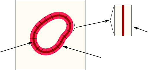
Figure 8: The tubular neighborhood $Y_{{\varepsilon}^{\prime}}=\cup_{i}Y_{{\varepsilon}^{\prime}}^{i}$ of $image(\tau)$ and the mapping $\phi^{i}:Y_{{\varepsilon}^{\prime}}^{i}\mapsto X_{{\varepsilon}^{\prime}}$.

6.2 Cutting into pieces

Choose a $C^{\infty}$ function $w_{2}:{\bf R}\mapsto[0,1]$ (cf. Section 5) supported in $[-1,1]$ so that

$$w_{2}(t/\rho)+w_{2}((t-1)/\rho)=1,\qquad-1/2\leq t\leq 0,$$

and

$$w_{2}(t/\rho)+w_{2}((t+1)/\rho)=1,\qquad 0\leq t\leq 1/2.$$

In addition, we require $w_{2}$ to satisfy

$$|\hat{w}_{2}(\omega)|\leq c\cdot e^{-|\omega|},\qquad\omega\in{\bf R}.$$ (6.2)

Define now a smooth partition of unity of $[0,1]$ using $w_{2}$:

$$w_{2,i}(t/\rho)=w_{2}((t-t_{i})/\rho),\qquad 1\leq i\leq m-1,$$

with a modification for $i\in\{0,m\}$ that depends on whether $\tau$ is closed or not. Then

$$\sum_{i}w_{2,i}(t/\rho)=1\qquad\forall t\in[0,1].$$ (6.3)

This will allow us to chop the curve $\tau$ into something that can be bent.

Now define the distributions

$${\cal C}^{i}=\int_{t_{i-1}}^{t_{i+1}}w_{2,i}(t/\rho)\delta_{\tau(t)}dt;$$

the partition of unity property (6.3) gives $\sum_{i}{\cal C}^{i}={\cal C}$.

We note that $\{\tau(t):t\in T^{i}\}\subset Y_{{\varepsilon}^{\prime}}^{i}$, and hence $\phi^{i}$ diffeomorphically straightens the piece of curve $\{\tau(t):t\in T^{i}\}$ into the line segment $\{0\}\times[-\rho,\rho]$.

6.3 Bending one piece

Now consider a diffeomorphism $\phi:{\bf R}^{2}\mapsto{\bf R}^{2}$; it acts on the distribution $f$ by change of variables

$$\phi^{\star}f=f\circ\phi.$$

This action induces a linear transformation on the space of curvelet coefficients. With $\alpha(f)$ the curvelet coefficients of $f$ and $\beta(f)$ the curvelet coefficients of $\phi^{\star}f$, we obtain a linear operator

$$M_{\phi}(\alpha(f))=\beta(f).$$

It is by now well-known that diffeomorphisms preserve sparsity of frame coefficients when the frame is based on parabolic scaling (as with curvelets and shearlets). For example, the following can be derived from Hart Smith’s work [38] by a simple atomic decomposition.

Lemma 6.2

[8, Theorem 6.1, page 219] For $p>0$, define the operator quasi-norm

$$\|M_{\phi}\|_{Op,p}=\max\left\{\sup_{\eta}\|(\langle\gamma_{\eta},\phi^{\star}\gamma_{\eta^{\prime}}\rangle)_{\eta}\|_{p},\sup_{\eta^{\prime}}\|(\langle\gamma_{\eta},\phi^{\star}\gamma_{\eta^{\prime}}\rangle)_{\eta^{\prime}}\|_{p}\right\}$$

Let $\phi$ denote a diffeomorphism that reduces to the identity outside of a compact set. Then for $0<p\leq 1$,

$$\|M_{\phi}\|_{Op,p}<c_{p}<\infty.$$

Far more detailed and precise results on the invariance of curvelet coefficients under $C^{2}$ changes of variables, with optimal regularity conditions, were developed by Candès and Demanet [5] – as we will see in the next section.

The $p$-triangle inequality $|a+b|^{p}\leq|a|^{p}+|b|^{p}$ for $p\in(0,1]$ implies the following:

Lemma 6.3

For $p\in(0,1]$, a vector $\alpha=(\alpha_{\eta})_{\eta}$, and a linear operator $M$,

$$\|M\alpha\|_{p}\leq\|M\|_{Op,p}\|\alpha\|_{p}.$$

6.4 Gluing pieces together

Now define

$$\beta_{j}=(\langle\gamma_{\eta},{\cal C}_{j}\rangle)_{\eta}.$$

From the decomposition ${\cal C}_{j}=\sum_{i=1}^{m}{\cal C}^{i}_{j}$ we have

$$\beta_{j}=\sum_{i=1}^{m}M_{\phi^{i}}\alpha_{j}.$$

This decomposition allows us to relate sparsity of coefficients of the linear singularity to those of the curvilinear singularity:

$$\|\beta_{j}\|_{p} \leq m^{1/p}\cdot\left(\max_{i}\|M_{\phi^{i}}\|_{Op,p}\right)\cdot\|\alpha_{j}\|_{p}.$$

This decomposition will be useful below; however, the above argument, which implies sparsity, will not be enough for our main result, which requires also to know the geometric arrangement of the significant coefficients. The next section develops a much finer estimation approach.

7 The cluster ${\cal S}_{2,j}$ and its estimates

We finally turn to the definition of the cluster set ${\cal S}_{2,j}$ and the decisive estimates

$$\delta_{2,j}=o(\|f_{j}\|_{2}),\qquad j\rightarrow\infty,$$ (7.1)

and

$$\mu_{c}({\cal S}_{2,j},\{\gamma_{\eta}\};\{\psi_{\lambda}\})\rightarrow 0,\qquad j\rightarrow\infty.$$ (7.2)

As explained in Section 2.2, combining these results with the results of Section 4 will complete the proof of Theorem 1.1.

We define the cluster of curvelet coefficients indirectly. We first define $\tilde{{\cal S}}_{j}$, the cluster of significant coefficients of our ‘straight’ model singularity $w{\cal L}_{j}$; then by cutting, bending, and filtering, we induce a cluster for the curvilinear singularity ${\cal C}_{j}$. Set

$$\tilde{{\cal S}}_{j}=\{(j,k,\ell)\in\Delta_{j}^{\pm 1}:(b_{j,k,\ell},\theta_{j,\ell})\in{\mathcal{N}}_{2}^{PS}(a_{j})\}.$$ (7.3)

Lemma 5.4 shows that this set contains the significant coefficients of $w{\cal L}_{j}$.

Let $M_{F_{j}}=(\langle\gamma_{\eta},F_{j}\star\gamma_{\eta^{\prime}}\rangle)_{\eta,\eta^{\prime}}$ be the filtering matrix associated with the filter $F_{j}$, and recall the definition of the mapping matrix $M_{(\phi^{i})^{-1}}$ from Subsection 6.3. Our analysis will require us to consider their product, hence for the sake of brevity we define $M_{j}^{i}$ to be

$$M_{j}^{i}=M_{F_{j}}\cdot M_{(\phi^{i})^{-1}}$$

and the entries of this matrix by $M_{j}^{i}(\eta,\eta^{\prime})$. Further, we let $t_{\eta^{\prime},n}$ denote the amplitude of the $n$’th largest element of the $\eta^{\prime}$’th column. Also let $n_{j}=2^{j{\varepsilon}}$, where ${\varepsilon}$ was fixed at the beginning of Section 4. We can think of ${\varepsilon}$ being arbitrarily small, however for our analysis the condition ${\varepsilon}<1/28$ will be sufficient.

Morally, what we would like to do is study a cluster of curvelet coefficients built from the cluster pieces

$${\cal S}_{j}^{i}=\{\eta:\eta^{\prime}\in\tilde{{\cal S}}_{j}\mbox{ and }|M_{j}^{i}(\eta,\eta^{\prime})|>t_{\eta^{\prime},n_{j}}\}.$$

In words, ${\cal S}_{j}^{i}$ consists of the ‘top-$n_{j}$’ curvelet coefficients affected by some significant coefficient in $\tilde{{\cal S}}_{j}$. The overall cluster set would then be made by combing the pieces:

$${\cal S}_{2,j}=\bigcup_{i}{\cal S}_{j}^{i}.$$

While this morally explains what we do in this section, it turns out that the exact behavior of ${\cal S}_{j}^{i}$ and ${\cal S}_{2,j}$ defined in this natural manner would be rather delicate. In fact, this section uses a more robust definition of cluster set that is similar in spirit; see (7.6)-(7.7) below. This definition depends on some more sophisticated ideas, which we now develop.

7.1 Decay Estimates for the Curvelet Representation of FIO’s

We first recall some results from [5] on sparsity of curvelet representations of Fourier Integral Operators (FIO’s) and decay estimates of such a representation, which will later on be applied to the matrix $M_{j}^{i}$.

In order to state decay estimates of the curvelet representation of FIO’s, we first require a notion of distance between two curvelet indices. A suitable distance has first been introduced by Hart Smith in [38]. Our analysis will employ results obtained by Candès and Demanet in their work on the curvelet representation of wave propagators [5], in which they use the following variation of Hart Smith’s distance:

$$d_{HS}(\eta,\eta^{\prime})=|\theta_{j,\ell}-\theta_{j^{\prime},\ell^{\prime}}|^{2}+|b_{k}-b_{k^{\prime}}|^{2}+|\langle e_{\eta},b_{k}-b_{k^{\prime}}\rangle|,$$

where

$$b_{k}=R_{\theta_{j,\ell}}D_{a_{j}}k\quad\mbox{and}\quad e_{\eta}=(\cos(\theta_{j,\ell}),\sin(\theta_{j,\ell})),$$

and the difference $|\theta_{j,\ell}-\theta_{j^{\prime},\ell^{\prime}}|$ is understood to refer to geodesic distance in ${\bf P}^{1}$. In [5], this distance was then extended to derive a distance adapted to discrete curvelet indices, which means, in particular, including the scaling component. For a pair of curvelet indices $\eta=(j,k,\ell)$ and $\eta^{\prime}=(j^{\prime},k^{\prime},\ell)$, this so-called dyadic-parabolic pseudo-distance is defined by

$$\omega(\eta,\eta^{\prime})=2^{|j-j^{\prime}|}\left(1+\min\{2^{j},2^{j^{\prime}}\}d_{HS}(\eta,\eta^{\prime})\right).$$

We will require the following property of this pseudo-distance:

Lemma 7.1

[5, Prop. 2.2 (3.)] For sufficiently large $N>0$, there is a constant $c_{N}>0$ such that

$$\sum_{\eta^{\prime\prime}}\omega(\eta,\eta^{\prime\prime})^{-N}\cdot\omega(\eta^{\prime\prime},\eta^{\prime})^{-N}\leq c_{N}\cdot\omega(\eta,\eta^{\prime})^{-(N-1)},\qquad\forall\eta,\eta^{\prime}.$$

Another property which will come in handy is the following estimate:

Lemma 7.2

[5, Proof of Thm. 1.1] There exist some $N>0$ and constant $c_{N}>0$ obeying

$$\sum_{\eta}\omega(\eta,\eta^{\prime})^{-N}\leq c_{N},\qquad\forall\eta,\eta^{\prime}.$$

Before we can state the next result we have to briefly recall some of the key notions in microlocal analysis. Let $S^{\star}({\bf R}^{2})$ denote the cosphere bundle of ${\bf R}^{2}$ – roughly speaking $\{(b_{0},\theta_{0}):b_{0}\in{\bf R}^{2},\,\theta_{0}\in{\bf P}^{1}\}$ –, and let $\phi$ be a diffeomorphism of ${\bf R}^{2}$. Then the associated so-called canonical transformation $\chi$ maps some element $(b_{0},\theta_{0})$ of phase space into $\chi(b_{0},\theta_{0})=(\phi(b_{0}),\phi^{\star}\theta_{0})$, where $\phi^{\star}\theta_{0}$ is the codirection into which the codirection $\theta_{0}$ based infinitesimally at $b_{0}$ is mapped under $\phi$. Phrasing it differently, we can say that each diffeomorphism of the base space ${\bf R}^{2}$ induces a diffeomorphism of phase space. Such a canonical transformation induces a mapping of curvelet indices which – abusing notation – we again denote by $\chi$. Since we will consider discrete curvelet coefficients $\eta$, we have to be careful how to define this extension. In fact, we will define the image of $\eta$ to be the closest point using the pseudo-distance $\omega$ to the image of $\eta$ under the canonical transformation. As already remarked in [5], choosing a different neighbor only affects the constants in the key inequalities.

The basic insights about parabolic scaling and FIO’s are already present in [38], implying sparsity of FIO’s of order $0$, as explained in [8]. But utilizing the dyadic-parabolic pseudo-distance, Candès and Demanet derived phase space decay estimates for the curvelet representation of FIO’s of each order $m$, which imply sparsity, but also inform about geometry.

Theorem 7.1

[5, Thm. 5.1] Let $T$ be a Fourier Integral Operator of order $m$ acting on functions of ${\bf R}^{2}$. Then, for each $N>0$, there exists some positive constant $c_{N}$ such that

$$|\langle\gamma_{\eta},T\gamma_{\eta^{\prime}}\rangle|\leq c_{N}\cdot 2^{mj^{\prime}}\omega(\eta,\chi(\eta^{\prime}))^{-N}.$$ (7.4)

Moreover, for each $0<p<\infty$, $(\langle\gamma_{\eta},T\gamma_{\eta^{\prime}}\rangle)$ is bounded from $\ell_{p}$ to $\ell_{p}$.

In the sequel we will use the first part of the result for $m=0$. Let us now turn to the decay estimate of the cluster approximate error $\delta_{2,j}$.

7.2 ${\cal S}_{2,j}$ offers low approximation error

In this section we give two decisive lemmas which drive our analysis, and define ${\cal S}_{2,j}$. From now on $\chi^{i}$ denotes the extension to curvelet indices of the canonical transformation associated with $(\phi^{i})^{-1}$.

Lemma 7.3

For any $N>0$, there exists a positive constant $c_{N}$ such that

$$|M_{j}^{i}(\eta,\eta^{\prime})|\leq c_{N}\cdot\omega(\eta,\chi^{i}(\eta^{\prime}))^{-N},\qquad\forall\eta,\eta^{\prime}.$$ (7.5)

Proof. Given $N>0$, by Theorem 7.1, there exists some positive constant $c_{N}$ such that (7.4) holds, which implies both

$$|\langle\gamma_{\eta},F_{j}\star\gamma_{\eta^{\prime}}\rangle|\leq c_{N}\cdot\omega(\eta,\eta^{\prime})^{-(N+1)}\quad\mbox{and}\quad|\langle\gamma_{\eta},\gamma_{\eta^{\prime}}\circ(\phi^{i})^{-1}\rangle|\leq c_{N}\cdot\omega(\eta,\chi^{i}(\eta^{\prime}))^{-(N+1)}.$$

Now applying Lemma 7.1 proves the claim. $\Box$

Lemma 7.4

There is a constant $c_{1}>0$ such that for each vector $\alpha=(\alpha_{\eta})_{\eta}$ ,

$$\|M_{j}^{i}\alpha\|_{1}\leq c_{1}\cdot\|\alpha\|_{1}.$$

Proof. This already follows from Lemma 6.3. However, it is instructive to reprove it using (7.5) of Lemma 7.3:

$$\|M_{j}^{i}\alpha\|_{1}\leq\sup_{\eta^{\prime}}\sum_{\eta}|M_{j}^{i}(\eta,\eta^{\prime})|\cdot\|\alpha\|_{1}\leq c_{N}\cdot\sup_{\eta^{\prime}}\sum_{\eta}\omega(\eta,\chi^{i}(\eta^{\prime}))^{-N}\cdot\|\alpha\|_{1}.$$

Realizing that the $\sup_{\eta^{\prime}}$ allows us to omit $\chi^{i}$ and applying Lemma 7.2,

$$\sup_{\eta^{\prime}}\sum_{\eta}\omega(\eta,\chi^{i}(\eta^{\prime}))^{-N}=\sup_{\eta^{\prime}}\sum_{\eta}\omega(\eta,\eta^{\prime})^{-N}\leq c_{N}.\qquad\mbox{$\Box$}$$

These two lemmas say that, in place of studying $M_{j}^{i}$ and its detailed properties, we can simply study its majorant $c_{N}\cdot\omega(\eta,\chi^{i}(\eta^{\prime}))^{-N}$. So fix $N$ large and let $\tilde{M}_{j}^{i}$ denote the ‘model’

$$\tilde{M}_{j}^{i}(\eta,\eta^{\prime})=c_{N}\cdot\omega(\eta,\chi^{i}(\eta^{\prime}))^{-N}.$$ (7.6)

We define our cluster set ${\cal S}_{2,j}$ in terms of the model rather than in terms of $M_{j}^{i}$, via

$${\cal S}_{2,j}=\bigcup_{i}{\cal S}_{j}^{i},$$ (7.7)

where

$${\cal S}_{j}^{i}=\{\eta:\eta^{\prime}\in\tilde{{\cal S}}_{j}\mbox{ and }|\tilde{M}_{j}^{i}(\eta,\eta^{\prime})|>t_{\eta^{\prime},n_{j}}\}.$$

In this definition, ${\cal S}_{j}^{i}$ is not truly the set of significant coefficients, but rather a set of sites where significant coefficients could potentially occur, given the geometry of the problem; so it is a bit larger. We still speak of ${\cal S}_{2,j}$ as if it were exactly the set of significant coefficients.

The set $\tilde{{\cal S}}_{j}$ is explicitly defined by a tube in phase space; the tube becomes narrower at finer scales and ‘converges’ to $WF(w{\cal L})$. The set of potentially significant coefficients ${\cal S}_{j}^{i}$ is a much thicker set and gets progressively thicker relative to $\tilde{{\cal S}}_{j}$ with increasing $j$, however, geometrically the corresponding ‘tube’ is still becoming very narrow as $j$ increases. This device already appeared in the Heuristics section; it allows to conveniently bound all the insignificant interactions $M_{j}^{i}(\eta,\eta^{\prime})$; in particular, see the estimate of $T_{2}$ in the proof of Lemma 7.5.

We can now prove the estimate (7.1) for the cluster approximate error $\delta_{2,j}$.

Lemma 7.5

$$\delta_{2,j}=o(\|f_{j}\|_{2}),\qquad j\rightarrow\infty.$$

Proof. As in Section 6.4, let $\beta_{j}=(\langle\gamma_{\eta},{\cal C}_{j}\rangle)_{\eta}$ as well as $\beta_{j}^{i}=(\langle\gamma_{\eta},{\cal C}^{i}_{j}\rangle)_{\eta}$, $i\in\{0,\ldots,m-1\}$. The decomposition ${\cal C}_{j}=\sum_{i}{\cal C}^{i}_{j}$ implies $\beta_{j}=\sum_{i}\beta_{j}^{i}$. Now

$$\sum_{\eta\in\Delta\setminus{\cal S}_{2,j}}|\beta_{j}(\eta)| \leq \sum_{i}\sum_{\eta\in\Delta_{j}^{\pm 1}\setminus{\cal S}_{j}^{i}}|\beta_{j}^{i}(\eta)|$$

$$\leq m\cdot\max_{i}\sum_{\eta\in\Delta_{j}^{\pm 1}\setminus{\cal S}_{j}^{i}}|\beta_{j}^{i}(\eta)|\leq m\cdot\max_{i}\|\beta_{j}^{i}\cdot 1_{\Delta_{j}^{\pm 1}\setminus{\cal S}_{j}^{i}}\|_{1}.$$

We now decompose $\|\beta_{j}^{i}\cdot 1_{\Delta_{j}^{\pm 1}\setminus{\cal S}_{j}^{i}}\|_{1}$ into three components and estimate each separately. Let $u_{j}:=\lceil{\varepsilon}\cdot j\rceil$ which will be the ‘radius’ of the scale-neighborhood about scale $j$ that we distinguish from the remaining (unimportant) scales. In what follows, remember the definition of $\tilde{{\cal S}}_{j}$ in (7.3); and let $\tilde{{\cal S}}_{j}^{\pm u_{j}}=\bigcup_{j^{\prime}}\tilde{{\cal S}}_{j^{\prime}}$ . Then

$$\|\beta_{j}^{i}\cdot 1_{\Delta_{j}^{\pm 1}\setminus{\cal S}_{j}^{i}}\|_{1}$$ (7.8)

$$\leq \|\tilde{M}_{j}^{i}(\alpha\cdot 1_{\Delta_{j}^{\pm u_{j}}\setminus\tilde{{\cal S}}_{j}^{\pm u_{j}}})\cdot 1_{\Delta_{j}^{\pm 1}\setminus{\cal S}_{j}^{i}}\|_{1}+\|\tilde{M}_{j}^{i}(\alpha\cdot 1_{\tilde{{\cal S}}_{j}^{\pm u_{j}}})\cdot 1_{\Delta_{j}^{\pm 1}\setminus{\cal S}_{j}^{i}}\|_{1}$$

$$+\|\tilde{M}_{j}^{i}(\alpha\cdot 1_{\Delta\setminus\Delta_{j}^{\pm u_{j}}})\cdot 1_{\Delta_{j}^{\pm 1}\setminus{\cal S}_{j}^{i}}\|_{1}$$

$$= T_{1}+T_{2}+T_{3}.$$

First, let’s estimate $T_{1}$. From Lemma 7.4, we obtain

$$T_{1}\leq\sum_{j^{\prime}=j-u_{j}}^{j+u_{j}}\|\tilde{M}_{j}^{i}(\alpha\cdot 1_{\Delta_{j^{\prime}}\setminus\tilde{{\cal S}}_{j^{\prime}}})\|_{1}\leq c_{1}\cdot\sum_{j^{\prime}=j-u_{j}}^{j+u_{j}}\|\alpha\cdot 1_{\Delta_{j^{\prime}}\setminus\tilde{{\cal S}}_{j^{\prime}}}\|_{1}.$$

By Lemma 5.4,

$$\|\alpha\cdot 1_{\Delta_{j^{\prime}}\setminus\tilde{{\cal S}}_{j^{\prime}}}\|_{1}=O(1),\qquad j^{\prime}\to\infty;$$

hence,

$$T_{1}\leq c_{1}\cdot(2u_{j}+1)=O(2^{j{\varepsilon}}),\qquad j\to\infty.$$ (7.9)

Next, turn to $T_{2}$. Observe that

$$T_{2}\leq\sum_{j^{\prime}=j-u_{j}}^{j+u_{j}}\Big{[}\sup_{\eta^{\prime}\in\tilde{{\cal S}}_{j^{\prime}}}\sum_{\eta\in\Delta_{j}^{\pm 1}\setminus{\cal S}_{j}^{i}}|\tilde{M}_{j}^{i}(\eta,\eta^{\prime})|\Big{]}\cdot\|\alpha\cdot 1_{\tilde{{\cal S}}_{j^{\prime}}}\|_{1}.$$ (7.10)

We now need the following standard lemma about $n$-term approximations.

Lemma 7.6

Let $x=(x_{i})_{i}$ denote a sequence of numbers and let $|x|_{(n)}$ denote the $n$th-largest element in the decreasing rearrangement. For $0<p<1$ we have the inequality:

$$\sum_{i}|x_{i}|\cdot 1_{\{|x_{i}|\leq|x|_{(n)}\}}\leq c_{p}\cdot\|x\|_{p}\cdot n^{-(1-p)/p},\quad n=1,2,\dots.$$

Recalling that ${\cal S}_{j}^{i}$ consists of elements $\eta$ such that $|\tilde{M}_{j}^{i}(\eta,\eta^{\prime})|>t_{\eta^{\prime},n_{j}}$, we conclude

$$\sup_{\eta^{\prime}\in\tilde{{\cal S}}_{j^{\prime}}}\sum_{\eta\in\Delta_{j}^{\pm 1}\setminus{\cal S}_{j}^{i}}|\tilde{M}_{j}^{i}(\eta,\eta^{\prime})|\leq c_{p}\cdot\left(\sup_{\eta^{\prime}}\sum_{\eta}|\tilde{M}_{j}^{i}(\eta,\eta^{\prime})|^{p}\right)^{1/p}\cdot n_{j}^{-(1-p)/p}\leq c_{1}\cdot c_{p}\cdot n_{j}^{-(1-p)/p}.$$

Also, from Lemma 5.3, we obtain $\|\alpha\cdot 1_{\tilde{{\cal S}}_{j^{\prime}}}\|_{1}\leq\|\alpha\cdot 1_{\Delta_{j^{\prime}}}\|_{1}\leq\tilde{c}_{1}2^{j^{\prime}(3/4+\epsilon)}$. Choose $p$ so that $p<4{\varepsilon}/(3+7{\varepsilon})$; returning to (7.10),

$$T_{2}\leq c\cdot n_{j}^{-(1-p)/p}\sum_{j^{\prime}=j-u_{j}}^{j+u_{j}}2^{j^{\prime}(3/4+\epsilon)}\leq c\cdot 2^{-(1-p){\varepsilon}j/p}\cdot(2u_{j}+1)\cdot 2^{3(j+u_{j})/4+j\epsilon}=O(2^{j{\varepsilon}}),\;j\to\infty,$$ (7.11)

At last, we consider $T_{3}$. Notice that

$$T_{3}\leq\sum_{|j-j^{\prime}|\geq u_{j}}\Big{[}\sup_{\eta^{\prime}\in\Delta_{j^{\prime}}}\sum_{\eta\in\Delta_{j}^{\pm 1}\setminus{\cal S}_{j}^{i}}|\tilde{M}_{j}^{i}(\eta,\eta^{\prime})|\Big{]}\cdot\|\alpha\cdot 1_{\Delta_{j^{\prime}}}\|_{1}.$$ (7.12)

Using the definition of $\tilde{M}_{j}$, we proceed as in the proof of Lemma 7.4, and employ the definition of the pseudo-distance $\omega$; we’ll obtain

$$\sup_{\eta^{\prime}\in\Delta_{j^{\prime}}}\sum_{\eta\in\Delta_{j}^{\pm 1}\setminus{\cal S}_{j}^{i}}|\tilde{M}_{j}^{i}(\eta,\eta^{\prime})| \leq \tilde{c}_{N}\cdot\sup_{\eta^{\prime}\in\Delta_{j^{\prime}}}\sum_{\eta\in\Delta_{j}^{\pm 1}\setminus{\cal S}_{j}^{i}}\omega(\eta,\eta^{\prime})^{-N}$$

$$\leq c\cdot 2^{-N|j-j^{\prime}|}.$$

By Lemma 5.3, the second term in (7.12) can be estimated by $\|\alpha\cdot 1_{\Delta_{j^{\prime}}}\|_{1}\leq c\cdot 2^{j^{\prime}(3/4+\epsilon)}$. We conclude that for $N$ sufficiently large,

$$T_{3}\leq c_{N}\sum_{|j-j^{\prime}|\geq u_{j}}2^{j^{\prime}(3/4+\epsilon)-N|j-j^{\prime}|}=O(2^{j{\varepsilon}}),\;j\to\infty.$$ (7.13)

Combining (7.9), (7.11), and (7.13) with (7.8) yields

$$\delta_{2,j}=\sum_{\eta\in({\cal S}_{j}^{i})^{c}}|\beta_{j}^{i}(\eta)|=O(2^{j{\varepsilon}})=o(\|f_{j}\|_{2}),\qquad j\rightarrow\infty.\quad\mbox{$\Box$}$$

7.3 ${\cal S}_{2,j}$ offers low cluster coherence

This section proves (7.2), the asymptotically negligible cluster coherence of ${\cal S}_{2,j}$.

Lemma 7.7

We have

$$\mu_{c}({\cal S}_{2,j},\{\gamma_{\eta}\};\{\psi_{\lambda}\})\rightarrow 0,\qquad j\rightarrow\infty.$$

Before giving the proof, we state two useful lemmas. Both use the variables $n_{j}$ introduced earlier. The first lemma implies that a given significant curvelet coefficient in the analysis of $w{\cal L}_{j}$ pushes forward to produce significant coefficients at roughly the same scale, and near a certain fixed orientation and location. Thus the pushforward acts roughly like a rigid motion. That first lemma is proved in Section 9.5.1.

Definition 7.1

Let the canonical transformation $\chi$ be given. For a specific curvelet index $\eta$ the forward set of radius $n$ is:

$$\mbox{\sc fwd}(\eta;\chi,n)=\{\eta^{\prime}:\omega(\eta^{\prime},\chi(\eta))\leq n\}.$$

In words, fwd is the set of curvelet indices close to the pushforward of $\eta$ by $\chi$. Note that the forward set covers the set of significant interactions with $\eta$:

$$\{\eta^{\prime}:|\tilde{M}_{j}^{i}(\eta^{\prime},\eta)|>t_{\eta,n_{j}}\}\subset\mbox{\sc fwd}(\eta;\chi^{i},n_{j}).$$

Consequently

$${\cal S}_{2,j}\subset\bigcup_{\eta\in\tilde{{\cal S}}_{j}}\bigcup_{i\in\{0,\dots,m\}}\mbox{\sc fwd}(\eta;\chi^{i},n_{j}).$$

Lemma 7.8

Let $\eta=(j,k,\ell)$ be a curvelet index, with its image under the canonical transformation $\chi^{i}$ denoted by $\chi^{i}(\eta)=(\tilde{j},\tilde{k},\tilde{\ell})$ for a fixed $i\in\{0,\ldots,m\}$. There exists some positive constant $c>0$ such that, for $j$ sufficiently large,

$$\mbox{\sc fwd}(\eta;\chi^{i},n_{j}) \subseteq \{(j^{\prime},k^{\prime},\ell^{\prime}):|j^{\prime}-\tilde{j}|\leq c\cdot\log n_{j},\,|2^{(j^{\prime}-\tilde{j})/2}\tilde{\ell}-\ell^{\prime}|^{2}\leq c\cdot n_{j},\,$$

$$2^{j^{\prime}}\cdot\max\{|b_{\tilde{k}}-b_{k^{\prime}}|^{2},|b_{\tilde{k}}-b_{k^{\prime}}|\}\leq c\cdot n_{j}\}$$

We conclude that for sufficiently large $j_{0}$, there exists $c>0$ so that

$$\#\mbox{\sc fwd}(\eta;\chi^{i},n_{j})\leq c\cdot n_{j}^{4},\qquad j>j_{0},\quad\eta\in\tilde{{\cal S}}_{j}.$$

Let $k(\eta)$ denote the $k$-component of $\eta=(j,k,\ell)$. Define

$$d_{min}(\eta,i,n_{j})=\min\{|k(\eta^{\prime})|:\eta^{\prime}\in\mbox{\sc fwd}(\eta;\chi^{i},n_{j})\}.$$

We also need the fact that points in the forward set of $\eta$ have spatial components almost as far from the origin as the spatial component of $\eta$ itself.

Lemma 7.9

There are $j_{0},c_{1,0},c_{2,0}$ so that we have

$$d_{min}(\eta;i,n_{j})\geq c_{1}(j)|k(\eta)|-c_{2}(j),\qquad j>j_{0},$$

where

$$c_{1}(j)=c_{1,0}/n_{j}\quad\mbox{ and }\qquad c_{2}(j)=c_{2,0}\cdot n_{j}.$$

The proof is given in the appendix, as is the proof of

Lemma 7.10

For $N>2$, there are constants $c_{3}$,$c_{4}$,$c_{5}$ such that

$$\sum_{k\in{\bf Z}^{2}}\langle(a|k|-b)_{+}\rangle^{-N}\leq(b/a)^{2}\cdot(c_{3}+c_{4}b^{-N})+c_{5}.$$

With the last three lemmas we can now prove the main result of this section.

Proof of Lemma 7.7. The definition of ${\cal S}_{2,j}$ implies

$$\mu_{c}({\cal S}_{2,j},\{\gamma_{\eta}\};\{\psi_{\lambda}\}) = \max_{j^{\prime},k^{\prime}}\sum_{\eta\in{\cal S}_{2,j}}|\langle\gamma_{\eta},\psi_{j^{\prime},k^{\prime}}\rangle|=\max_{j^{\prime},k^{\prime}}\sum_{i=0}^{m-1}\sum_{\eta\in{\cal S}_{j}^{i}}|\langle\gamma_{\eta},\psi_{j^{\prime},k^{\prime}}\rangle|$$

$$\leq m\cdot\max_{i}\max_{j^{\prime},k^{\prime}}\sum_{\eta\in{\cal S}_{j}^{i}}|\langle\gamma_{\eta},\psi_{j^{\prime},k^{\prime}}\rangle|$$

WLOG assume that $j^{\prime}=j$ and $k^{\prime}=0$, reducing the task to proving that $\sum_{\eta\in{\cal S}_{j}^{i}}|\langle\gamma_{\eta},\psi_{j,0}\rangle|\to 0$ as $j\to\infty$ for all $i$. We have the estimate

$$\mu_{c}({\cal S}_{2,j},\{\gamma_{\eta}\};\{\psi_{\lambda}\})\leq m\cdot\max_{i}\sum_{\eta\in{\cal S}_{j}^{i}}|\langle\gamma_{\eta},\psi_{j,0}\rangle|.$$ (7.14)

We can now continue (7.14) by applying Lemma 3.3 and the three lemmas immediately above:

$$\sum_{\eta\in{\cal S}_{j}^{i}}|\langle\gamma_{\eta},\psi_{j,0}\rangle| \leq \sum_{\eta\in\tilde{{\cal S}}_{j}}\sum_{\eta^{\prime}\in\mbox{\sc fwd}(\eta)}|\langle\gamma_{\eta^{\prime}},\psi_{j,0}\rangle|$$

$$\leq \sum_{\eta\in\tilde{{\cal S}}_{j}}\sum_{\eta^{\prime}\in\mbox{\sc fwd}(\eta)}c_{N}\cdot 2^{-j/4}\cdot\langle|k(\eta^{\prime})|\rangle^{-N}$$

$$\leq c\cdot 2^{-j/4}\cdot\sum_{\eta\in\tilde{{\cal S}}_{j}}\#\mbox{\sc fwd}(\eta)\cdot\langle d_{min}(\eta)\rangle^{-N}$$

$$\leq c\cdot 2^{-j/4}\cdot n_{j}^{4}\cdot\sum_{\eta\in\tilde{{\cal S}}_{j}}\langle(c_{1}(j)|k(\eta)|-c_{2}(j))_{+}\rangle^{-N}$$

$$\leq c\cdot 2^{-j/4}\cdot n_{j}^{4}\cdot\left(\frac{c_{2}(j)^{2}}{c_{1}(j)^{2}}\cdot(c_{3}+c_{4}\cdot c_{1}(j)^{2}(c_{2}(j))^{-N})+c_{5}\right)$$

$$\leq c\cdot 2^{-j/4}\cdot n_{j}^{8},\qquad j>j_{0}.$$

We have assumed that ${\varepsilon}<1/32$, so $2^{-j/4}n_{j}^{8}=2^{-j/4}\cdot 2^{8{\varepsilon}j}\rightarrow 0$ as $j\rightarrow\infty$; substituting this into (7.14) proves the lemma. $\Box$

8 Discussion

8.1 Extensions

So far we focused entirely on a very special separation problem using very specific tools of harmonic analysis. Our goal was to show that a certain set of questions and results make sense and provide insight. This is the ‘tip of the iceberg’: the main results are susceptible of very extensive generalizations and extensions.

• More General Classes of Objects. We may vary the problem, taking point and curve singularities whose ‘strength’ is different than the ones we chose in (1.1)-(1.2); however, always matching the strength of the point singularity to that of the curve singularity. For example, consider a ‘cartoon’ image model, where ${\cal C}$ is a function smooth away from discontinuities, and the components of the continuity set are bounded by a complex of smooth curves. Such cartoons still exhibit curvilinear singularities, but the singularities are of order zero rather than order $-1$. For a separation problem with nontrivial asymptotics, we replace the point singularity $|x-x_{i}|^{-3/2}$ in (1.1) by $|x-x_{i}|^{-1/2}$, preserving an energy-matching condition like (1.3), with $r^{-1}$ replacing $r^{1}$. Recall that, without energy matching, the whole problem is trivial. With such changes the proof of Theorem 1.1 will run very closely in parallel. As a general rule, if $\langle{\cal C},f\rangle=\int(\triangle^{\gamma}f)(\tau(t))dt$, where $\gamma$ is a fractional power of the Laplacian $\triangle$, then matching point singularities have strength $\alpha=(-3+4\gamma)/2$. The case we studied in this paper was $\gamma=0$ and hence $\alpha=-3/2$.

• Other Frame Pairs. Theorem 1.1 holds without change for many other pairs of frames and bases. Consider this pair:

  • Orthonormal Separable Meyer Wavelets – an orthonormal basis of perfectly isotropic generating elements.

  • Shearlets – a highly directional tight frame with increasingly anisotropic elements at fine scales.

  In this pair, the wavelets are actually orthonormal, and both wavelets and shearlets correspond very closely to discrete transforms used in digital image processing. In digital image processing, the notions of ‘radial’, ‘directional’, ‘rotation’ and so on are problematic; both orthonormal wavelets and shearlets avoid such concepts. At the same time this pair offers the same ability to sparsify point and curve singularities as the counterparts pair we introduced above. This allows to provide a complete methodology for the continuous and discrete setting (see, e.g., [28, 31]) as well as for algorithmic realizations (see, e.g., [33, 32]).

  While the proof arguments explicitly cover the one frame pair we have taken pains to define so far, those arguments extend immediately to other ‘compatible’ pairs – where the cross-frame matrices are almost diagonal in a suitable sense. This grants us the freedom to prove results in one system which is convenient, but apply those to another compatible system. The arguments showing that shearlets and curvelets are compatible are supplied in [21]. In this paper we discussed the pair radial wavelets/curvelets. However, all results hold true in a similar way for the pair orthonormal wavelets/shearlets.

• Noisy Data. Are the results studied here robust against small modelling errors? In fact they are. Consider an image composed of ${\cal P}$ and ${\cal C}$ with additive noise ${\mathcal{N}}$, hence we measure $\tilde{f}={\cal P}+{\cal C}+{\mathcal{N}}$ instead of $f$. We then – as in the noiseless case – filter to obtain subband components $\tilde{f}_{j}={\cal P}_{j}+{\cal C}_{j}+{\mathcal{N}}_{j}$ and apply $(\mbox{CSep})$ to $\tilde{f}_{j}$ to obtain a pair $(\tilde{W}_{j},\tilde{C}_{j})$. Provided that the noise component ${\mathcal{N}}$ has ‘sufficiently’ small curvelet coefficients in the sense that at each scale $j$ the $\ell_{1}$ norm of the analysis coefficients satisfies $o(2^{j/2})$ as $j\to\infty$, we again obtain asymptotically perfect separation:

  $$\frac{\|\tilde{W}_{j}-{\cal P}_{j}\|_{2}+\|\tilde{C}_{j}-{\cal C}_{j}\|_{2}}{\|{\cal P}_{j}\|_{2}+\|{\cal C}_{j}\|_{2}}\rightarrow 0,\qquad j\rightarrow\infty$$

  This can be proved along the lines of the proof of Theorem 1.1. Indeed, consider a composed signal $\tilde{S}=S_{1}^{0}+S_{2}^{0}+n$ with components $S_{1}^{0}$ and $S_{2}^{0}$ relatively sparse as in Proposition 2.1, and noise term $n$ satisfying $\|\Phi_{1}^{T}n\|_{1}<{\varepsilon}$ or $\|\Phi_{2}^{T}n\|_{1}<{\varepsilon}$. Let $(\tilde{S}_{1}^{\star},\tilde{S}_{2}^{\star})$ solve (2.1) with $S$ substituted by $\tilde{S}$. Then following the proof of Proposition 2.1 line by line and adapting the arguments accordingly shows:

  $$\|\tilde{S}_{1}^{\star}-S_{1}^{0}\|_{2}+\|\tilde{S}_{2}^{\star}-S_{2}^{0}\|_{2}\leq\frac{2\delta+5{\varepsilon}}{1-2\kappa}.$$ (8.1)

  Substituting Proposition 2.1 by estimate (8.1) in the proof of Theorem 1.1 implies the result on geometric separation of noisy data stated in Subsection 8.1.

  We conclude that our analysis is indeed stable.

• Rate of Convergence. One might wonder about the rate of separation. The lemmas proven in Sections 4-7 imply the following upper bound on the rate of convergence for $\ell_{1}$ minimization:

  $$\frac{\|W_{j}-{\cal P}_{j}\|_{2}+\|C_{j}-{\cal C}_{j}\|_{2}}{\|{\cal P}_{j}\|_{2}+\|{\cal C}_{j}\|_{2}}=O(2^{-j(1/2-\epsilon)}),\qquad j\rightarrow\infty.$$

  Such information might be the key to getting even stronger separation conclusions.

• Other Algorithms and Other Notions of Separation. In the companion paper [20] we show that one pass of alternating hard thresholding, properly tuned, can achieve asymptotic separation. Surprisingly, we can even show clean separation at the level of wavefront sets.

8.2 Interpretation as an Uncertainty Principle

Separation results such as the ‘birth problem’ of $\ell_{1}$ component separation, a combination of sinusoids and spikes [18], have been interpreted at that time as uncertainty principles. As a reminder to the reader, the classical uncertainty principle states that a signal cannot be highly concentrated in both time and frequency; and a lower bound is placed on the product of the concentration in time and in frequency. The core property which allows the separation of sinusoids and spikes by using a dictionary consisting of the unit basis and the Fourier basis, is the non-existence of a sparse representation of a signal both in time and in frequency.

Considering the present separation problem, these core ideas need to be extended, thereby providing us with yet another interpretation than the one already presented in the previous sections. The two representation ‘domains’ are now the isotropic system of wavelets and the anisotropic system of curvelets. Hence, we might regard the separation result of Theorem 1.1 as a statement that a 2D Schwartz distribution cannot be sparsely represented via analysis coefficients both in the ‘isotropic world’ and in the ‘anisotropic world’. In particular, if a 2D Schwartz distribution has a sparse representation in wavelets, it is not sparse in curvelets and vice versa. Phrasing it in more general terms, a 2D Schwartz distribution having only isotropic features cannot be sparsely represented using an anisotropic system, and if it has only exhibits anisotropic phenomena, it does not possess a sparse representation in terms of an isotropic system.

Summarizing, comparison with the classical uncertainty principle shows that we here derive an uncertainty principle for the isotropy-anisotropy relation instead of the classical time-frequency relation.

9 Proofs

9.1 Proofs of Results from Section 2

9.1.1 Proof of Proposition 2.1

Proof. Since $\Phi_{1}$ and $\Phi_{2}$ are tight frames,

$$\|S_{1}^{\star}-S_{1}^{0}\|_{2}+\|S_{2}^{\star}-S_{2}^{0}\|_{2} = \|\Phi_{1}^{T}(S_{1}^{\star}-S_{1}^{0})\|_{2}+\|\Phi_{2}^{T}(S_{2}^{\star}-S_{2}^{0})\|_{2}$$

$$\leq \|\Phi_{1}^{T}(S_{1}^{\star}-S_{1}^{0})\|_{1}+\|\Phi_{2}^{T}(S_{2}^{\star}-S_{2}^{0})\|_{1}.$$

Now invoke exact decomposition: $S_{1}^{0}+S_{2}^{0}=S=S_{1}^{\star}+S_{2}^{\star}$. Rewrite the last display:

$$\|S_{1}^{\star}-S_{1}^{0}\|_{2}+\|S_{2}^{\star}-S_{2}^{0}\|_{2}\leq\|\Phi_{1}^{T}(S_{1}^{\star}-S_{1}^{0})\|_{1}+\|\Phi_{2}^{T}(S_{1}^{\star}-S_{1}^{0})\|_{1}.$$

By definition of $\kappa$,

$$\|\Phi_{1}^{T}(S_{1}^{\star}-S_{1}^{0})\|_{1}+\|\Phi_{2}^{T}(S_{1}^{\star}-S_{1}^{0})\|_{1}$$

$$= \|1_{{\cal S}_{1}}\Phi_{1}^{T}(S_{1}^{\star}-S_{1}^{0})\|_{1}+\|1_{{\cal S}_{2}}\Phi_{2}^{T}(S_{1}^{\star}-S_{1}^{0})\|_{1}+\|1_{{\cal S}_{1}^{c}}\Phi_{1}^{T}(S_{1}^{\star}-S_{1}^{0})\|_{1}+\|1_{{\cal S}_{2}^{c}}\Phi_{2}^{T}(S_{2}^{\star}-S_{2}^{0})\|_{1}$$

$$\leq \kappa\cdot\left(\|\Phi_{1}^{T}(S_{1}^{\star}-S_{1}^{0})\|_{1}+\|\Phi_{2}^{T}(S_{1}^{\star}-S_{1}^{0})\|_{1}\right)+\|1_{{\cal S}_{1}^{c}}\Phi_{1}^{T}(S_{1}^{\star}-S_{1}^{0})\|_{1}+\|1_{{\cal S}_{2}^{c}}\Phi_{2}^{T}(S_{2}^{\star}-S_{2}^{0})\|_{1};$$

use relative sparsity of the subsignals $S_{i}^{0}$, $i=1,2$,

$$\|\Phi_{1}^{T}(S_{1}^{\star}-S_{1}^{0})\|_{1}+\|\Phi_{2}^{T}(S_{1}^{\star}-S_{1}^{0})\|_{1}$$ (9.1)

$$\leq \frac{1}{1-\kappa}(\|1_{{\cal S}_{1}^{c}}\Phi_{1}^{T}(S_{1}^{\star}-S_{1}^{0})\|_{1}+\|1_{{\cal S}_{2}^{c}}\Phi_{2}^{T}(S_{2}^{\star}-S_{2}^{0})\|_{1})$$

$$\leq \frac{1}{1-\kappa}(\|1_{{\cal S}_{1}^{c}}\Phi_{1}^{T}S_{1}^{\star}\|_{1}+\|1_{{\cal S}_{1}^{c}}\Phi_{1}^{T}S_{1}^{0}\|_{1}+\|1_{{\cal S}_{2}^{c}}\Phi_{2}^{T}S_{2}^{\star}\|_{1}+\|1_{{\cal S}_{2}^{c}}\Phi_{2}^{T}S_{2}^{0}\|_{1})$$

$$\leq \frac{1}{1-\kappa}\left(\|1_{{\cal S}_{1}^{c}}\Phi_{1}^{T}S_{1}^{\star}\|_{1}+\|1_{{\cal S}_{2}^{c}}\Phi_{2}^{T}S_{2}^{\star}\|_{1}+\delta\right).$$

Apply minimality of $S_{1}^{\star}$ and $S_{2}^{\star}$,

$$\|1_{{\cal S}_{1}^{c}}\Phi_{1}^{T}S_{1}^{\star}\|_{1}+\|1_{{\cal S}_{1}}\Phi_{1}^{T}S_{1}^{\star}\|_{1}+\|1_{{\cal S}_{2}^{c}}\Phi_{2}^{T}S_{2}^{\star}\|_{1}+\|1_{{\cal S}_{2}}\Phi_{2}^{T}S_{2}^{\star}\|_{1} = \|\Phi_{1}^{T}S_{1}^{\star}\|_{1}+\|\Phi_{2}^{T}S_{2}^{\star}\|_{1}$$

$$\leq \|\Phi_{1}^{T}S_{1}^{0}\|_{1}+\|\Phi_{2}^{T}S_{2}^{0}\|_{1}.$$

Again use sparsity of the subsignals $S_{i}^{0}$, $i=1,2$,

$$\|1_{{\cal S}_{1}^{c}}\Phi_{1}^{T}S_{1}^{\star}\|_{1}+\|1_{{\cal S}_{2}^{c}}\Phi_{2}^{T}S_{2}^{\star}\|_{1}$$

$$\leq \|\Phi_{1}^{T}S_{1}^{0}\|_{1}+\|\Phi_{2}^{T}S_{2}^{0}\|_{1}-\|1_{{\cal S}_{1}}\Phi_{1}^{T}S_{1}^{\star}\|_{1}-\|1_{{\cal S}_{2}}\Phi_{2}^{T}S_{2}^{\star}\|_{1}$$

$$\leq \|\Phi_{1}^{T}S_{1}^{0}\|_{1}+\|\Phi_{2}^{T}S_{2}^{0}\|_{1}+\|1_{{\cal S}_{1}}\Phi_{1}^{T}(S_{1}^{\star}-S_{1}^{0})\|_{1}-\|1_{{\cal S}_{1}}\Phi_{1}^{T}S_{1}^{0}\|_{1}$$

$$+\|1_{{\cal S}_{2}}\Phi_{2}^{T}(S_{2}^{\star}-S_{2}^{0})\|_{1}-\|1_{{\cal S}_{2}}\Phi_{2}^{T}S_{2}^{0}\|_{1}$$

$$\leq \|1_{{\cal S}_{1}}\Phi_{1}^{T}(S_{1}^{\star}-S_{1}^{0})\|_{1}+\|1_{{\cal S}_{2}}\Phi_{2}^{T}(S_{2}^{\star}-S_{2}^{0})\|_{1}+\delta.$$

Using (9.1), this leads to

$$\|\Phi_{1}^{T}(S_{1}^{\star}-S_{1}^{0})\|_{1}+\|\Phi_{2}^{T}(S_{1}^{\star}-S_{1}^{0})\|_{1}$$

$$\leq \frac{1}{1-\kappa}\left[\|1_{{\cal S}_{1}}\Phi_{1}^{T}(S_{1}^{\star}-S_{1}^{0})\|_{1}+\|1_{{\cal S}_{2}}\Phi_{2}^{T}(S_{1}^{\star}-S_{1}^{0})\|_{1}+2\delta\right]$$

$$\leq \frac{1}{1-\kappa}\left[\kappa\cdot(\|\Phi_{1}^{T}(S_{1}^{\star}-S_{1}^{0})\|_{1}+\|\Phi_{2}^{T}(S_{1}^{\star}-S_{1}^{0})\|_{1})+2\delta\right].$$

Thus, finally we obtain

$$\|S_{1}^{\star}-S_{1}^{0}\|_{2}+\|S_{2}^{\star}-S_{2}^{0}\|_{2}\leq\left(1-\frac{\kappa}{1-\kappa}\right)^{-1}\cdot\frac{2\delta}{1-\kappa}=\frac{2\delta}{1-2\kappa}.\Box$$

9.1.2 Proof of Lemma 2.1

Proof. For each $f$, we choose coefficient sequences $\alpha_{1}$ and $\alpha_{2}$ such that $f=\Phi_{1}\alpha_{1}=\Phi_{2}\alpha_{2}$ and $\|\alpha_{i}\|_{1}\leq\|\beta_{i}\|_{1}$ for all $\beta_{i}$ satisfying $f=\Phi_{i}\beta_{i}$, $i=1,2$. Then, employing the fact that, because $\Phi_{1}$ and $\Phi_{2}$ are tight frames, also $f=\Phi_{i}\Phi_{i}^{T}\Phi_{i}\alpha_{i}$, $i=1,2$, we obtain

$$\|1_{{\cal S}_{1}}\Phi_{1}^{T}f\|_{1}+\|1_{{\cal S}_{2}}\Phi_{2}^{T}f\|_{1}$$

$$= \|1_{{\cal S}_{1}}\Phi_{1}^{T}\Phi_{2}\alpha_{2}\|_{1}+\|1_{{\cal S}_{2}}\Phi_{2}^{T}\Phi_{1}\alpha_{1}\|_{1}$$

$$\leq \sum_{i\in{\cal S}_{1}}\left(\sum_{j}|\langle\phi_{1,i},\phi_{2,j}\rangle||\alpha_{2,j}|\right)+\sum_{j\in{\cal S}_{2}}\left(\sum_{i}|\langle\phi_{1,i},\phi_{2,j}\rangle||\alpha_{1,i}|\right)$$

$$= \sum_{j}\left(\sum_{i\in{\cal S}_{1}}|\langle\phi_{1,i},\phi_{2,j}\rangle|\right)|\alpha_{2,j}|+\sum_{i}\left(\sum_{j\in{\cal S}_{2}}|\langle\phi_{1,i},\phi_{2,j}\rangle|\right)|\alpha_{1,i}|$$

$$\leq \mu_{c}({\cal S}_{1},\Phi_{1};\Phi_{2})\|\alpha_{2}\|_{1}+\mu_{c}({\cal S}_{2},\Phi_{2};\Phi_{1})\|\alpha_{1}\|_{1}$$

$$\leq \max\{\mu_{c}({\cal S}_{1},\Phi_{1};\Phi_{2}),\mu_{c}({\cal S}_{2},\Phi_{2};\Phi_{1})\}(\|\alpha_{1}\|_{1}+\|\alpha_{2}\|_{1})$$

$$\leq \max\{\mu_{c}({\cal S}_{1},\Phi_{1};\Phi_{2}),\mu_{c}({\cal S}_{2},\Phi_{2};\Phi_{1})\}(\|\Phi_{1}^{T}\Phi_{1}\alpha_{1}\|_{1}+\|\Phi_{2}^{T}\Phi_{2}\alpha_{2}\|_{1})$$

$$= \max\{\mu_{c}({\cal S}_{1},\Phi_{1};\Phi_{2}),\mu_{c}({\cal S}_{2},\Phi_{2};\Phi_{1})\}(\|\Phi_{1}^{T}f\|_{1}+\|\Phi_{2}^{T}f\|_{1}).$$

$\Box$

9.2 Proofs of Results from Section 3

9.2.1 Proof of Lemma 3.3

Using Parseval, $\langle\gamma_{a,b,\theta},\psi_{a_{0},b_{0}}\rangle=2\pi\int\hat{\gamma}_{a,b,\theta}(\xi)\hat{\psi}_{a_{0},b_{0}}(\xi)d\xi$, we consider

$$\int\hat{\gamma}_{a,b,\theta}(\xi)\hat{\psi}_{a_{0},b_{0}}(\xi)d\xi\ =\int a_{0}W(a_{0}r)e^{-ib_{0}^{\prime}\xi}\cdot a^{3/4}W(ar)V((\omega-\theta)/\sqrt{a})e^{-ib^{\prime}\xi}d\xi.$$

Now WLOG we may consider the special case $\theta=0$, so that $R_{\theta}=I$. Recall that $W$ is supported on $[1/2,2]$ by construction. Then

$$W(a_{0}r)W(ar)=0\qquad\forall r\geq 0,|\log_{2}(a/a_{0})|\geq 3.$$

Hence we need only consider the case where $|\log_{2}(a/a_{0})|<3$, and in that circumstance we may WLOG take $a=a_{0}$. We may also assume $b_{0}=0$. Apply the change of variables $\zeta=D_{a}\xi$ and $d\zeta=a^{3/2}d\xi$,

$$\int\hat{\gamma}_{a,b,\theta}(\xi)\hat{\psi}_{a,b_{0}}(\xi)d\xi=a^{1/4}\cdot\int W^{2}(\|\zeta_{a}\|)V(\omega(\zeta_{a})/\sqrt{a})e^{-i(D_{1/a}b)^{\prime}\zeta}d\zeta,$$

where $\zeta_{a}=(\zeta_{1},\sqrt{a}\zeta_{2})$ and $\omega(\zeta_{a})$ denotes the angular component of the polar coordinates of $\zeta_{a}$. Applying integration by parts, for any $k=1,2,...$,

$$|\langle\gamma_{a,b,\theta},\psi_{a_{0},b_{0}}\rangle| = 2\pi\cdot a^{1/4}\cdot|D_{1/a}b|^{-k}\left|\int\Delta^{k}[W^{2}(\|\zeta_{a}\|)V(\omega(\zeta_{a})/\sqrt{a})]e^{-i(D_{1/a}b)^{\prime}\zeta}d\zeta\right|$$

$$\leq 2\pi\cdot a^{1/4}\cdot|D_{1/a}b|^{-k}\int\left|\Delta^{k}[W^{2}(\|\zeta_{a}\|)V(\omega(\zeta_{a})/\sqrt{a})]\right|d\zeta.$$

Hence

$$(1+|D_{1/a}b|^{k})\cdot|\langle\gamma_{a,b,\theta},\psi_{a_{0},b_{0}}\rangle|$$ (9.2)

$$\leq 2\pi\cdot a^{1/4}\int\left[\left|W^{2}(\|\zeta_{a}\|)\right|\left|V(\omega(\zeta_{a})/\sqrt{a})\right|+\left|\Delta^{k}[W^{2}(\|\zeta_{a}\|)V(\omega(\zeta_{a})/\sqrt{a})]\right|\right]d\zeta.$$

Next we show that, for each $k$, there exists $c_{k}<\infty$ such that

$$\int\left[\left|W^{2}(\|\zeta_{a}\|)\right|\left|V(\omega(\zeta_{a})/\sqrt{a})\right|+\left|\Delta^{k}[W^{2}(\|\zeta_{a}\|)V(\omega(\zeta_{a})/\sqrt{a})]\right|\right]d\zeta\leq c_{k},\quad\forall\;a>0.$$ (9.3)

We have

$$\frac{\partial}{\partial\zeta_{1}}W^{2}(\|\zeta_{a}\|)=\frac{\partial}{\partial\zeta_{1}}W^{2}(\|(\,\cdot\,,\sqrt{a}\zeta_{2})\|)(\zeta_{1})$$

and

$$\frac{\partial}{\partial\zeta_{2}}W^{2}(\|\zeta_{a}\|)=\sqrt{a}\cdot\frac{\partial}{\partial\zeta_{2}}W^{2}(\|(\zeta_{1},\sqrt{a}\,\cdot\,)\|)(\zeta_{2}).$$

Hence, by induction, the absolute values of the derivatives of $W^{2}(\|\zeta_{a}\|)$ are upper bounded independently of $a$. Also,

$$\frac{\partial}{\partial\zeta_{1}}V(\omega(\zeta_{a})/\sqrt{a})=\frac{\partial}{\partial\zeta_{1}}V(\omega((\,\cdot\,,\zeta_{2})_{a})/\sqrt{a})(\zeta_{1})\cdot g_{1}(\zeta,a)$$

and

$$\frac{\partial}{\partial\zeta_{2}}V(\omega(\zeta_{a})/\sqrt{a})=\frac{\partial}{\partial\zeta_{2}}V(\omega((\zeta_{1},\,\cdot\,)_{a})/\sqrt{a})(\zeta_{1})\cdot g_{2}(\zeta,a),$$

and tedious computations show that both $|g_{1}|,|g_{2}|$ possess an upper bound independently of $a$. Thus, by induction, the absolute values of the derivatives of $V(\omega(\zeta_{a})/\sqrt{a})$ are upper bounded independently of $a$. These observations imply (9.3).

Further, for each $k=1,2,..$,

$$\langle|D_{1/a}b|\rangle^{k}=(1+|D_{1/a}b|^{2})^{\frac{k}{2}}\leq\frac{k}{2}(1+|D_{1/a}b|^{k}).$$ (9.4)

To finish, simply combine (9.2), (9.3), and (9.4), and recall that we chose coordinates so that $\theta=0$. Translating back to the case of general $\theta$ gives the full conclusion. $\Box$

9.3 Proofs of Results from Section 4

9.3.1 Proof of Lemma 4.1

Proof. By Parseval,

$$\langle\psi_{a_{j^{\prime}},b},{\cal P}_{j}\rangle=2\pi\int\hat{\psi}_{a_{j^{\prime}},b}(\xi)\hat{{\cal P}}_{j}(\xi)d\xi=2\pi\int a_{j^{\prime}}W(a_{j^{\prime}}r)e^{-ib^{\prime}\xi}W(a_{j}r)r^{-1/2}d\xi,$$

where of course $r=|\xi|$. Now

$$W(a_{j^{\prime}}r)W(a_{j}r)=0\qquad\forall r\geq 0,\qquad|j-j^{\prime}|>1,$$

hence we may as well assume that $j^{\prime}=j$. Making the change of variables $\zeta=a_{j}\xi$, $d\zeta=a_{j}^{2}d\xi$ and defining the annulus ${\cal A}=\{\zeta:1/2\leq|\zeta|\leq 2\}$,

$$\langle\psi_{a_{j},b},{\cal P}_{j}\rangle=2\pi\cdot a_{j}^{-1/2}\cdot\int_{{\cal A}}W^{2}(|\zeta|)|\zeta|^{-1/2}e^{-i(b/a_{j})^{\prime}\zeta}d\zeta.$$

Applying integration by parts, for any $k=0,1,...$,

$$|\langle\psi_{a_{j},b},{\cal P}_{j}\rangle| = 2\pi\cdot a_{j}^{-1/2}\cdot|b/a_{j}|^{-k}\cdot\left|\int_{\cal A}\Delta^{k}[W^{2}(|\zeta|)|\zeta|^{-1/2}]e^{-i(b/a_{j})^{\prime}\zeta}d\zeta\right|$$

$$\leq 2\pi\cdot a_{j}^{-1/2}\cdot|b/a_{j}|^{-k}\cdot\int_{\cal A}\left|\Delta^{k}[W^{2}(|\zeta|)|\zeta|^{-1/2}]\right|d\zeta.$$

Hence

$$(1+|b/a_{j}|^{k})\cdot|\langle\psi_{a_{j},b},{\cal P}_{j}\rangle|\leq 2\pi\cdot a_{j}^{-1/2}\cdot\int_{\cal A}\left[\left|W^{2}(|\zeta|)|\zeta|^{-1/2}\right|+\left|\Delta^{k}[W^{2}(|\zeta|)|\zeta|^{-1/2}]\right|\right]d\zeta.$$ (9.5)

For $W$ suitably chosen,

$$\int_{\cal A}\left[\left|W^{2}(|\zeta|)|\zeta|^{-1/2}\right|+\left|\Delta^{k}[W^{2}(|\zeta|)|\zeta|^{-1/2}]\right|\right]d\zeta<\infty.$$

Further, for each $k=1,2,..$,

$$\langle|b/a_{j}|\rangle^{k}=(1+|b/a_{j}|^{2})^{\frac{k}{2}}\leq\frac{k}{2}(1+|b/a_{j}|^{k}).$$

Infusing these two last observations into (9.5), for any $N=1,2,...$,

$$|\langle\psi_{a_{j^{\prime}},b},{\cal P}_{j}\rangle|\leq c_{N}\cdot a_{j}^{-1/2}\cdot 1_{|j-j^{\prime}|\leq 1}\cdot\langle|b/a_{j}|\rangle^{-N}.$$

$\Box$

9.4 Proofs of Results from Section 5

9.4.1 Proof of Lemma 5.1

We study the situation geometrically, and for each $(a,b,\theta)$ define the line segment

$$Seg(a,b,\theta)=\Big{\{}D_{1/a}R_{-\theta}\left(\begin{array}[]{c}-b_{1}\\ y-b_{2}\end{array}\right):|y|\leq\rho\Big{\}}.$$

Two special points associated to these line segments will play an essential role in our estimate; they are defined in

Lemma 9.1

Retain the definitions for $d_{1},d_{2},\sigma_{1},\sigma_{2},$ and $\tau$ from the statement of Lemma 5.1. Then, for each $a,b,\theta$, the following conditions are fulfilled.

• Consider the line

  $$Line(a,b,\theta)=\Big{\{}D_{1/a}R_{-\theta}\left(\begin{array}[]{c}-b_{1}\\ y-b_{2}\end{array}\right):y\in{\bf R}\Big{\}}.$$

  The closest point $P_{L}$ to the origin on $Line(a,b,\theta)$ satisfies

  $$\|P_{L}\|_{2}^{2}=b_{1}^{2}(\sigma_{2}^{2}-\sigma_{1}^{-2}\tau)=d_{1}^{2}.$$

• Let $P_{S}$ be the closest point on $Seg(a,b,\theta)$ to the origin. Then

  $$\|P_{S}-P_{L}\|_{2}^{2}=d_{2}^{2}.$$

Figure 9 shows a general configuration featuring $P_{L}$ and $P_{S}$.

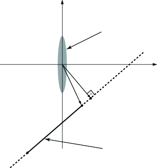
Figure 9: Relation between a curvelet $\gamma_{a,b,\theta}$, a line segment $Seg(a,b,\theta)$, its affine hull $Line(a,b,\theta)$, and the points $P_{L}$ and $P_{S}$.

Proof. Set

$$L(y):=D_{{1}/{a}}R_{-\theta}\left(\begin{array}[]{c}-b_{1}\\ y-b_{2}\end{array}\right).$$

Then

$$\|L(y)\|_{2}^{2} = \|(a^{-1}(-b_{1}\cos\theta+(y-b_{2})\sin\theta),a^{-1/2}(b_{1}\sin\theta+(y-b_{2})\cos\theta)\|_{2}^{2}$$ (9.6)

$$= b_{1}^{2}\sigma_{2}^{2}+(y-b_{2})^{2}\sigma_{1}^{2}+2b_{1}(y-b_{2})\tau.$$

Since

$$\frac{d}{dy}\|L(y)\|_{2}^{2}=2(y-b_{2})\sigma_{1}^{2}+2b_{1}\tau,$$

it follows by definition of $P_{L}$ that

$$P_{L}=L(b_{2}-\sigma_{1}^{-2}b_{1}\tau).$$ (9.7)

Hence, by (9.6),

$$d_{1}^{2}=\|P_{L}\|_{2}^{2}=b_{1}^{2}\sigma_{2}^{2}+(-\sigma_{1}^{-2}b_{1}\tau)^{2}\sigma_{1}^{2}+2b_{1}(-\sigma_{1}^{-2}b_{1}\tau)\tau=b_{1}^{2}(\sigma_{2}^{2}-\sigma_{1}^{-2}\tau).$$

This proves (i).

To prove (ii), observe that, by (9.7), $P_{L}\in Seg(a,b,\theta)$ if and only if $b_{2}-\sigma_{1}^{-2}b_{1}\tau\in[-\rho,\rho]$, which are the two different cases the definition of $d_{2}^{2}$ is separated into. Now, if $P_{L}\in Seg(a,b,\theta)$, then, obviously, $d_{2}^{2}=0$. Next assume that $P_{L}\not\in Seg(a,b,\theta)$. Then

$$d_{2}^{2} = \min_{\pm}\|L(\pm\rho)-P_{L}\|_{2}^{2}$$

$$= \min_{\pm}\;(\pm\rho-b_{2})^{2}\sigma_{1}^{2}+\sigma_{1}^{-4}b_{1}^{2}\tau^{2}\sigma_{1}^{2}+2(\rho-b_{2})\sigma_{1}^{-2}b_{1}\tau\sigma_{1}^{2}$$

$$= \min_{\pm}\;((\pm\rho-b_{2})\sigma_{1}-\sigma_{1}^{-1}b_{1}\tau)^{2}.$$

$\Box$

Now define the ray integral

$$R_{N}(x_{0},y_{0})=\int_{y_{0}}^{\infty}\langle|(x_{0},t)|\rangle^{-N}dt,$$

i.e., we integrate along the vertical ray ${\cal R}(x_{0},y_{0})$ whose ‘lowest’ point is $(x_{0},y_{0})$. The geometry of the previous lemma allows to control the curvelet coefficient of a linear singularity by a ray integral, properly deployed. Farther below we will prove:

Lemma 9.2

Let

$$\langle w{\cal L},\gamma_{a,b,\theta}\rangle=\int_{-\rho}^{\rho}w(x_{2}/\rho)\gamma_{a,b,\theta}(0,x_{2})dx$$

where $\|w\|_{\infty}\leq 1$. Then

$$|\langle w{\cal L},\gamma_{a,b,\theta}\rangle|\leq a^{-3/4}\cdot\sigma_{1}^{-1}\cdot R_{N}(d_{1},\sigma_{1}d_{2}).$$

The next lemma gives a bound on the ray integral which, combined with the last lemma, finishes the proof of Lemma 5.1.

Lemma 9.3

For $y_{0}\geq 0$,

$$R_{N}(x_{0},y_{0})\leq\pi\cdot\langle|x_{0}|\rangle^{-1}\cdot\langle|(x_{0},y_{0})|\rangle^{2-N}.$$ (9.8)

Proof of Lemma 9.3. For $\beta\in(0,1)$,

$$\int_{0}^{\infty}|f(t)|dt\leq(\sup_{t\in(0,\infty)}|f(t)|^{\beta})\cdot\int_{0}^{\infty}|f(t)|^{1-\beta}dt.$$

Now setting $(1-\beta)N=2$ and $f(t)=\langle|(x_{0},y_{0}+t)|\rangle^{-N}$, we have

$$R_{N}(x_{0},y_{0})\leq(\sup_{v\in{\cal R}(x_{0},y_{0})}\langle|v|\rangle^{2-N})\cdot\int_{0}^{\infty}|\langle|(x_{0},y_{0}+t)|\rangle^{-2}dt.$$

Since

$$\int_{-\infty}^{\infty}|\langle|(x_{0},y)|\rangle^{-M}dy=\langle|x_{0}|\rangle^{-M}\cdot\int_{-\infty}^{\infty}\langle y/\langle x_{0}\rangle\rangle^{-M}dy=\langle|x_{0}|\rangle^{-M+1}\cdot\int_{-\infty}^{\infty}\langle t\rangle^{-M}dt,$$

setting $M=2$ and recalling $\pi=\int_{-\infty}^{\infty}(1+t^{2})^{-1}dt$, it follows that

$$\int_{0}^{\infty}|\langle|(x_{0},y_{0}+t)|\rangle^{-2}dt\leq\pi\cdot\langle|x_{0}|\rangle^{-1}.$$

Meanwhile, since $y_{0}\geq 0$,

$$\sup_{v\in{\cal R}(x_{0},y_{0})}\langle|v|\rangle^{2-N}=\langle|(x_{0},y_{0})|\rangle^{2-N}.$$

This proves (9.8). $\Box$

Proof of Lemma 9.2. By Lemma 3.2, Lemma 9.1, and using the fact that $\|w\|_{\infty}\leq 1$,

$$|\langle w{\cal L},\gamma_{a,b,\theta}\rangle| = \Big{|}\int_{-\rho}^{\rho}w_{2}(y/\rho)\gamma_{a,b,\theta}(0,y)dy\Big{|}$$

$$\leq \int_{-\rho}^{\rho}|\gamma_{a,b,\theta}(0,y)|dy$$

$$\leq \int_{Seg(a,b,\theta)}a^{-3/4}\langle|v|\rangle^{-N}dv$$

where we used an affine transformation of variables to turn the anisotropic norm $|(0,y)|_{a,\theta}$ into the Euclidean norm $|v|$; the same transformation turns $\{0\}\times[-\rho,\rho]$ into $Seg(a,b,\theta)$. In the final expression, the integral is along a non-unit-speed curve traversing $Seg(a,b,\theta)$, at speed $\sigma_{1}$. Now let $Ray(a,b,\theta)$ denote the ray starting from $P_{S}$ and initially traversing $Seg(a,b,\theta)$. We continue with

$$c_{N}\cdot a^{-3/4}\cdot\int_{Seg(a,b,\theta)}\langle|v|\rangle^{-N}dv \leq c_{N}\cdot a^{-3/4}\cdot\int_{Ray(a,b,\theta)}\langle|v|\rangle^{-N}dv$$

$$= c_{N}\cdot a^{-3/4}\cdot\sigma_{1}^{-1}\int_{\sigma_{1}\cdot Ray(a,b,\theta)}\langle|w|\rangle^{-N}dw$$

$$= c_{N}\cdot a^{-3/4}\cdot\sigma_{1}^{-1}\int_{\sigma_{1}d_{2}}^{\infty}\langle|(d_{1},t)|\rangle^{-N}dt$$

$$= c_{N}\cdot a^{-3/4}\cdot\sigma_{1}^{-1}\cdot R_{N}(d_{1},\sigma_{1}d_{2}).$$

In (9.4.1), the integral involves a unit-speed curve traversing $Ray(a,b,\theta)$, which explains the appearance of the speed factor $\sigma_{1}$. $\Box$

9.4.2 Proof of Lemma 5.2

By definition of the line singularity $w{\cal L}$ and by (5.1), we can rewrite $\langle w{\cal L},\gamma_{a,b,\theta}\rangle$ in the following way:

$$2\pi\langle w{\cal L},\gamma_{a,b,\theta}\rangle=\int(\hat{w}\star\hat{\gamma}_{a,b,\theta})(\xi_{1},0)d\xi_{1}.$$ (9.10)

Since

$$(\hat{w}\star\hat{\gamma}_{a,b,\theta})(\xi)=\int\rho\cdot\hat{w}_{2}(\rho(\xi_{2}-\eta_{2}))\delta_{0}(\xi_{1}-\eta_{1})\hat{\gamma}_{a,b,\theta}(\eta)d\eta,$$

it follows that

$$(\hat{w}\star\hat{\gamma}_{a,b,\theta})(\xi_{1},0) = e^{ib_{1}\xi_{1}}\int\rho\cdot\hat{w}_{2}(-\rho\eta_{2})\hat{\gamma}_{a,0,\theta}(\xi_{1},\eta_{2})e^{ib_{2}\eta_{2}}d\eta_{2}.$$

By (9.10), this implies

$$2\pi\langle w{\cal L},\gamma_{a,b,\theta}\rangle=\int e^{ib_{1}\xi_{1}}\Big{[}\int\rho\cdot\hat{w}_{2}(-\rho\eta_{2})\hat{\gamma}_{a,0,\theta}(\xi_{1},\eta_{2})e^{ib_{2}\eta_{2}}d\eta_{2}\Big{]}d\xi_{1}.$$

Repeatedly applying integration by parts, and incorporating analyst’s brackets $\langle|\,\cdot\,|\rangle$ as in the proof of Lemma 4.1, we obtain

$$2\pi|\langle w{\cal L},\gamma_{a,b,\theta}\rangle|\leq\langle|b_{1}|\rangle^{-L}\cdot\langle|b_{2}|\rangle^{-M}\cdot\|h_{L,M}\|_{L^{1}({\bf R})},$$ (9.11)

where

$$h_{L,M}(\xi_{1})=\rho\cdot\int D^{L,M}\Big{(}\hat{w}_{2}(-\rho\eta_{2})\hat{\gamma}_{a,0,\theta}(\xi_{1},\eta_{2})e^{ib_{2}\eta_{2}}\Big{)}d\eta_{2}$$

and for some ‘nice’ $f\in L^{2}({\bf R}^{2})$,

$$D^{L,M}f(\eta_{1},\eta_{2})=\left(\frac{\partial}{\partial\eta_{1}}\right)^{L}\left(\frac{\partial}{\partial\eta_{2}}\right)^{M}f(\eta_{1},\eta_{2}).$$

Next, we will estimate the term $|h_{L,M}(\xi_{1})|$ from (9.11), and prove that

$$|h_{L,M}(\xi_{1})|\leq c\cdot a^{3/4}\cdot e^{-\rho\frac{|\sin\theta|}{2a}}\cdot(a^{1/2}|\sin\theta|+a|\cos\theta|)^{L}\cdot(\rho+a^{1/2}|\cos\theta|+a|\sin\theta|)^{M}.$$ (9.12)

Let $\Xi_{a,\theta}(\xi_{1})$ denote the support of the function $\xi_{1}\mapsto D^{L,M}(\hat{w}(\rho\eta_{2})\hat{\gamma}_{a,0,\theta}(\xi_{1},\eta_{2})e^{ib_{2}\eta_{2}})$. Then $h_{L,M}$ can be written as

$$h_{L,M}(\xi_{1})=\rho\cdot\int_{\Xi_{a,\theta}(\xi_{1})}D^{L,M}\Big{(}\hat{w}_{2}(-\rho\eta_{2})\hat{\gamma}_{a,0,\theta}(\xi_{1},\eta_{2})e^{ib_{2}\eta_{2}}\Big{)}d\eta_{2}.$$ (9.13)

We next rewrite the integrand as

$$D^{L,M}\Big{(}\hat{w}_{2}(-\rho\eta_{2})\hat{\gamma}_{a,0,\theta}(\xi_{1},\eta_{2})e^{ib_{2}\eta_{2}}\Big{)}$$

$$= \sum_{m=0}^{M}\left(\begin{array}[]{c}M\\ m\end{array}\right)\hat{w}^{(m)}_{2}(-\rho\eta_{2})(-\rho)^{m}D^{L,M-m}(\hat{\gamma}_{a,0,\theta}(\xi_{1},\eta_{2})e^{ib_{2}\eta_{2}}).$$

This allows us to estimate $|h_{L,M}(\xi_{1})|$ using (9.13) and (6.2) by

$$|h_{L,M}(\xi_{1})| \leq \sum_{m=0}^{M}\left(\begin{array}[]{c}M\\ m\end{array}\right)\Big{|}\int_{\Xi_{a,\theta}(\xi_{1})}\hat{w}^{(m)}_{2}(-\rho\eta_{2})(-\rho)^{m}D^{L,M-m}(\hat{\gamma}_{a,0,\theta}(\xi_{1},\eta_{2})e^{ib_{2}\eta_{2}})d\eta_{2}\Big{|}$$ (9.17)

$$\leq \sum_{m=0}^{M}\left(\begin{array}[]{c}M\\ m\end{array}\right)\rho^{m+1}\cdot\|\hat{w}^{(m)}_{2}(\rho\,\cdot)\|_{L^{1}[|\sin\theta|/(2a),\infty)}N^{L,M-m}(a,\theta)$$ (9.20)

$$\leq c\cdot\sum_{m=0}^{M}\left(\begin{array}[]{c}M\\ m\end{array}\right)\rho^{m+1}\cdot e^{-\rho\frac{|\sin\theta|}{2a}}\cdot N^{L,M-m}(a,\theta),$$ (9.23)

where

$$N^{L,M-m}(a,\theta)=\|D^{L,M-m}\hat{\gamma}_{a,0,\theta}(\xi_{1},\eta_{2})\|_{L^{\infty}(\Xi_{a,\theta}(\xi_{1}))}.$$

Since, by simple decay estimates,

$$|D_{1}^{L}\hat{\gamma}_{a,0,\theta}(\eta_{1},\eta_{2})|\leq C_{L}\cdot a^{3/4}\cdot(a|\cos\theta|+a^{1/2}|\sin\theta|)^{L}$$

and

$$|D_{2}^{M}\hat{\gamma}_{a,0,\theta}(\eta_{1},\eta_{2})|\leq C_{M}\cdot a^{3/4}\cdot(a^{1/2}|\cos\theta|+a|\sin\theta|)^{M},$$

the term $N^{L,M-m}(a,\theta)$ can be estimated by

$$N^{L,M-m}(a,\theta)\leq c_{L,M}\cdot a^{3/4}\cdot(a|\cos\theta|+a^{1/2}|\sin\theta|)^{L}(a^{1/2}|\cos\theta|+a|\sin\theta|)^{M}.$$

Combining this finding with (9.23) proves (9.12).

Thus, in particular, by the support of the function $h_{L,M}$, the $L^{1}$-norm of this function can be estimated as

$$\|h_{L,M}\|_{L^{1}({\bf R})}$$

$$\leq c\cdot a^{-1}\cdot|\cos\theta|\cdot a^{3/4}\cdot e^{-\rho\frac{|\sin\theta|}{2a}}\cdot(a^{1/2}|\sin\theta|+a|\cos\theta|)^{L}\cdot(\rho+a^{1/2}|\cos\theta|+a|\sin\theta|)^{M}.$$

Combining this estimate with (9.11) yields

$$|\langle w{\cal L},\gamma_{a,b,\theta}\rangle| \leq c_{M,L}\cdot a^{-1/4}\cdot|\cos\theta|\cdot e^{-\rho\frac{|\sin\theta|}{2a}}\cdot\langle|b_{1}|\rangle^{-L}\cdot(a^{1/2}|\sin\theta|+a|\cos\theta|)^{L}$$

$$\cdot\langle|b_{2}|\rangle^{-M}\cdot(\rho+a^{1/2}|\cos\theta|+a|\sin\theta|)^{M},$$

as claimed. $\Box$

9.5 Proofs of Results from Section 7

9.5.1 Proof of Lemma 7.8

Proof. Below, various constants will appear, which for simplicity shall all be denoted by $c$. Also we write $b_{\tilde{k}}$, $b_{k^{\prime}}$, etc. in place of the full notation $b_{\tilde{j},\tilde{k},\tilde{\ell}}=R_{\theta_{j,\ell}}D_{2^{-j}}k$, etc. Throughout the proof we associate $\tilde{\eta}$ with the triple $(\tilde{j},\tilde{k},\tilde{\ell})$ and similarly for $\eta^{\prime}$ and $(j^{\prime},k^{\prime},\ell^{\prime})$.

Suppose first that $j^{\prime}\geq\tilde{j}$. Then

$$\omega(\eta^{\prime},\tilde{\eta})$$

$$= 2^{|\tilde{j}-j^{\prime}|}\left(1+\min\{2^{\tilde{j}},2^{j^{\prime}}\}\left[|\theta_{\tilde{j},\tilde{\ell}}-\theta_{j^{\prime},\ell^{\prime}}|^{2}+|b_{\tilde{k}}-b_{k^{\prime}}|^{2}+|\langle e_{\eta^{\prime}},b_{\tilde{k}}-b_{k^{\prime}}\rangle|\right]\right)$$

$$\leq c\cdot\left(2^{j^{\prime}-\tilde{j}}+|\tilde{\ell}-2^{(\tilde{j}-j^{\prime})/2}\ell^{\prime}|^{2}+2^{\tilde{j}}\cdot|b_{\tilde{k}}-b_{k^{\prime}}|^{2}+2^{\tilde{j}}|\langle e_{\eta^{\prime}},b_{\tilde{k}}-b_{k^{\prime}}\rangle|\right).$$

Similarly, if $j^{\prime}<\tilde{j}$:

$$\omega(\eta^{\prime},\tilde{\eta}) \leq c\cdot\left(2^{\tilde{j}-j^{\prime}}+|2^{(j^{\prime}-\tilde{j})/2}\tilde{\ell}-\ell^{\prime}|^{2}+2^{j^{\prime}}\cdot|b_{\tilde{k}}-b_{k^{\prime}}|^{2}+2^{j^{\prime}}|\langle e_{\eta^{\prime}},b_{\tilde{k}}-b_{k^{\prime}}\rangle|\right).$$ (9.24)

Using the model (7.6), we now seek to prove that, for sufficiently large $j$,

$$\#\{\eta^{\prime}:|\tilde{M}_{j}^{i}(\eta^{\prime},\eta)|\geq c_{N}\cdot n_{j}^{-N}\}=\#\{\eta^{\prime}:\omega(\eta^{\prime},(\tilde{j},\tilde{k},\tilde{\ell}))\leq n_{j}\}\geq n_{j}.$$ (9.25)

We first study the case $j^{\prime}<\tilde{j}$. Let $\tilde{\omega}(\eta^{\prime},\tilde{\eta})$ denote the RHS of (9.24). Note that, if we can prove (9.25) with $\tilde{\omega}(\eta^{\prime},\tilde{\eta})$ in place of $\omega(\eta^{\prime},\tilde{\eta})$, this immediately implies the original claim of (9.25). We repeatedly use the (trivial)

Lemma 9.4

For each fixed $x\in{\bf R}$, the set of $k\in{\bf Z}$ satisfying $|k-x|\leq R$ has cardinality $\geq R-1$.

Define $C_{j,j^{\prime},\tilde{j}}=n_{j}/c-2^{j^{\prime}-\tilde{j}}$, where $c$ is the constant in (9.24). The condition $\tilde{\omega}\leq n_{j}$ is equivalent to

$$\|2^{(j^{\prime}-\tilde{j})/2}\tilde{\ell}-\ell^{\prime}|^{2}+2^{j^{\prime}}\cdot|b_{\tilde{k}}-b_{k^{\prime}}|^{2}+2^{j^{\prime}}|\langle e_{\eta^{\prime}},b_{\tilde{k}}-b_{k^{\prime}}\rangle| \leq C_{j,j^{\prime},\tilde{j}}.$$ (9.26)

We next derive conditions making each of the three terms smaller than $C_{j,j^{\prime},\tilde{j}}/3$, thus implying (9.26). Fix $j^{\prime}$. By Lemma 9.4, there are at least $C_{j,j^{\prime},\tilde{j}}^{1/2}/\sqrt{3}-1$ integer values $\ell^{\prime}\in{\bf Z}$ obeying

$$|2^{(j^{\prime}-\tilde{j})/2}\tilde{\ell}-\ell^{\prime}|^{2}\leq\frac{1}{3}C_{j,j^{\prime},\tilde{j}}.$$ (9.27)

Now, define $\tilde{x}=\tilde{x}(\tilde{\eta},\eta^{\prime})=R_{\theta_{j^{\prime},\ell^{\prime}}}^{-1}b_{\tilde{k}}$. Since $R_{\theta_{j^{\prime},\ell^{\prime}}}$ is an isometry,

$$|b_{\tilde{k}}-b_{k}|^{2}=|\tilde{x}-D_{2^{-j^{\prime}}}k^{\prime}|^{2}.$$

At the same time,

$$|\langle e_{\eta^{\prime}},b_{\tilde{k}}-b_{k^{\prime}}\rangle|=|\tilde{x}_{1}-2^{-j^{\prime}}k_{1}^{\prime}|.$$

Now there are at least $C_{j,j^{\prime},\tilde{j}}^{1/2}/\sqrt{6}-1$ integers $k_{2}^{\prime}\in{\bf Z}$ obeying

$$|2^{j^{\prime}/2}\tilde{x}_{2}-k^{\prime}_{2}|\leq C_{j,j^{\prime},\tilde{j}}^{1/2}/\sqrt{6}.$$ (9.28)

For large $j^{\prime}$, there are at least $C_{j,j^{\prime},\tilde{j}}/3-1$ integers $k_{1}^{\prime}\in{\bf Z}$ obeying both

$$|2^{j^{\prime}}\tilde{x}_{1}-k^{\prime}_{1}|\leq 2^{j^{\prime}/2}\cdot C_{j,j^{\prime},\tilde{j}}^{1/2}/\sqrt{6}$$

and

$$|2^{j^{\prime}}\tilde{x}_{1}-k^{\prime}_{1}|\leq C_{j,j^{\prime},\tilde{j}}/3.$$ (9.29)

Every pair $k^{\prime}=(k^{\prime}_{1},k^{\prime}_{2})\in{\bf Z}^{2}$ satisfying the conditions (9.28)-(9.29) simultaneously, satisfies

$$|b_{\tilde{k}}-b_{k}|^{2}\leq C_{j,j^{\prime},\tilde{j}}/3\quad\mbox{and}\quad|\langle e_{\eta^{\prime}},b_{\tilde{k}}-b_{k^{\prime}}\rangle|\leq C_{j,j^{\prime},\tilde{j}}/3.$$ (9.30)

Combining the above displays, we have at least $(C_{j,j^{\prime},\tilde{j}}/3-1)\cdot(C_{j,j^{\prime},\tilde{j}}^{1/2}/\sqrt{6}-1)$ points $k^{\prime}=(k^{\prime}_{1},k^{\prime}_{2})\in{\bf Z}^{2}$ satisfying (9.30). Every pair $(k^{\prime},\ell^{\prime})$ satisfying (9.30) and (9.27) satisfies (9.26). So focusing just on $j^{\prime}=j$, we obtain a large number of pairs $(k^{\prime},\ell^{\prime})$ satisfying (9.26): $\geq c\cdot C_{j,j^{\prime},\tilde{j}}^{2}\sim c\cdot n_{j}^{2}\gg n_{j}$ such pairs. In particular, for all large $j$, inequality $\omega(\tilde{\eta},\eta^{\prime})\leq n_{j}$ is satisfied by at least $n_{j}$ triples $\eta^{\prime}=(j^{\prime},k^{\prime},\ell^{\prime})$.

For the case $j^{\prime}<\tilde{j}$, using (9.24), we can similarly prove that $\omega\leq n_{j}$ is satisfied by at least $n_{j}$ triples $(j^{\prime},k^{\prime},\ell^{\prime})$.

Finally, we observe that $\omega(\tilde{\eta},\eta^{\prime})\leq n_{j}$ can only hold if

$$|j^{\prime}-\tilde{j}|\leq c\cdot\log n_{j},\quad|2^{(j^{\prime}-\tilde{j})/2}\tilde{\ell}-\ell^{\prime}|\leq c\cdot n_{j}$$ (9.31)

and

$$2^{j^{\prime}}\cdot\max\{|b_{\tilde{k}}-b_{k^{\prime}}|^{2},|b_{\tilde{k}}-b_{k^{\prime}}|\}\leq c\cdot n_{j}.$$ (9.32)

Concluding, each $\eta^{\prime}$ contained in the sets in (9.25) must satisfy both (9.31) and (9.32). $\Box$

9.5.2 Proof of Lemma 7.9

For $\eta\in\tilde{{\cal S}}_{j}$, we have $\theta=0$ and $|b_{2}|<n_{j}/2^{j}$ while $|b_{1}|<2\rho/2^{j/2}$. WLOG suppose that, for the patch $i$ in question, we have that the $\eta^{\prime}\in S_{j}^{i}$ of interest has $b^{\prime}=R_{\theta^{\prime}}D_{2^{-j^{\prime}}}k^{\prime}$ for some $\theta$ obeying $|\theta|\leq cn_{j}/2^{j/2}$. For such a pair $(\eta,\eta^{\prime})$, note that

$$k=D_{2^{j}}R_{0}^{-1}b,\qquad k^{\prime}=D_{2^{j^{\prime}}}R_{\theta^{\prime}}^{-1}b^{\prime};$$

it is also convenient to define $x^{\prime}=D_{2^{j-j^{\prime}}}k^{\prime}$. Then

$$k_{2}-x^{\prime}_{2}=2^{j/2}\left((1-\cos(\theta^{\prime}))b_{2}^{\prime}+(b_{2}-b^{\prime}_{2})-\sin(\theta^{\prime})b^{\prime}_{1}\right).$$

Now $|b^{\prime}_{1}|<C$ for $\eta^{\prime}\in\mbox{\sc fwd}(\eta)$, and, from Lemma 7.8 we infer

$$|1-\cos(\theta^{\prime})|<cn_{j}^{2}/2^{j},\qquad|b^{\prime}_{2}-b_{2}|<cn_{j}/2^{j},\qquad|\sin(\theta^{\prime})|<cn_{j}/2^{j/2}.$$

Combining these,

$$|k_{2}-x^{\prime}_{2}|<2cn_{j}^{2},$$

so $|x^{\prime}_{2}|>|k_{2}|-2cn_{j}^{2}$, and

$$|k^{\prime}_{2}|=2^{(j^{\prime}-j)/2}|x^{\prime}_{2}|\geq 2^{-|j-j^{\prime}|/2}\cdot\left(|k_{2}|-2cn_{j}^{2}\right).$$

Now $2^{|j-j^{\prime}|}<cn_{j}$ for $\eta^{\prime}\in\mbox{\sc fwd}(\eta)$, so $|k(\eta)|\leq|k_{2}(\eta)|+|k_{1}(\eta)|\leq|k_{2}(\eta)|+cn_{j}$, for $\eta\in\tilde{{\cal S}}_{j}$. So

$$|k(\eta^{\prime})|\geq|k^{\prime}_{2}|\geq 2^{-|j-j^{\prime}|/2}\cdot\left(|k_{2}|-2cn_{j}^{2}\right),\qquad j>j_{0}.$$

$\Box$

9.5.3 Proof of Lemma 7.10

Let $Q_{\ell}$ denote the square of sidelength $2^{\ell}+1$ centered at the origin. Within each annulus $A_{\ell}=Q_{\ell}-Q_{\ell-1}$ there are, for $\ell\geq 2$, fewer than $2^{2\ell}$ points in the annulus and each one has $\ell^{2}$ norm at least $2^{\ell-2}$. Partition the sum $\sum_{{\bf Z}^{2}}=\sum_{Q_{1}+A_{2}+A_{3}+\dots}$. Starting at $\ell=2$ each annulus contributes at most $2^{2\ell}\cdot\langle(a2^{\ell-2}-b)_{+}\rangle^{-N}$ to the sum, and the inner square $Q_{1}$ contributes at most 9. Then

$$\sum_{k\in{\bf Z}^{2}}\langle(a|k|-b)_{+}\rangle^{-N} \leq 9+\sum_{m=2}^{\infty}2^{2\ell}\cdot\langle(a2^{\ell-2}-b)_{+}\rangle^{-N}$$

$$= 9+16\cdot\left(\sum_{m=0}^{\infty}2^{2m}\cdot\langle(a2^{m}-b)_{+}\rangle^{-N}\right).$$

Let $m_{0}$ satisfy $2b\geq a2^{m_{0}}\geq b$. Now

$$T_{1}:=\sum_{m=0}^{m_{0}}2^{2m}\langle|a2^{m}-b|_{+}\rangle^{-N} \leq \sum_{m=0}^{m_{0}}2^{2m}\leq 2^{2m_{0}+1}.$$

Now $2^{2m_{0}}\leq(2b/a)^{2}$, so $2^{m_{0}}\leq 2b/a$. So $T_{1}\leq 2\cdot(2b/a)^{2}$.

On the other hand, $a2^{m}-b\geq 0$ for $m\geq m_{0}$, while $a2^{m-m_{0}}\leq a2^{m}-b$. Then

$$T_{2}:=\sum_{m>m_{0}}2^{2m}\langle|a2^{m-m_{0}}|\rangle^{-N} \leq \sum_{m=m_{0}+1}^{\infty}2^{2m}(a2^{m-m_{0}})^{-N}$$

$$\leq 2^{2(m_{0}+1)}(a2^{-m_{0}})^{N}\sum_{h=0}^{\infty}2^{2h}2^{-hN}$$

$$= 2^{m_{0}(2-N)}\cdot a^{N}\cdot 2\cdot(1-2^{-(N-2)})^{-1}$$

$$\leq (b/a)^{2-N}\cdot a^{N}\cdot 4$$

$$\leq 4\cdot(2b/a)^{2}\cdot b^{-N}$$

Hence

$$T_{1}+T_{2}\leq(b/a)^{2}\cdot\left(8+16b^{-N}\right).$$

Combining these displays gives the lemma, with explicit constants. $\Box$

References

- [1] J. Bobin, J.-L. Starck, M.J. Fadili, Y. Moudden, and D.L. Donoho, Morphological Component Analysis: An Adaptive Thresholding Strategy, IEEE Trans. Image Proc. 16(11) (2007), 2675–2681.
- [2] L. Borup, R. Gribonval, and M. Nielsen, Beyond Coherence : Recovering Structured Time-Frequency Representations, Appl. Comput. Harmon. Anal. 24(1) (2008), 120–128.
- [3] A.M. Bruckstein, D.L. Donoho, and M. Elad, From Sparse Solutions of Systems of Equations to Sparse Modeling of Signals and Images, SIAM Review 51(1) (2009), 34–81.
- [4] F. Bunea, A. Tsybakov and M. Wegkamp, Aggregation for Gaussian Regression, Annals of Statistics 35(4) (2007), 1674–1697.
- [5] E. J. Candès and L. Demanet, The curvelet representation of wave propagators is optimally sparse, Comm. Pure Appl. Math. 58(11) (2005), 1472–1528.
- [6] E. J. Candès and D. L. Donoho, New tight frames of curvelets and optimal representations of objects with singularities, Comm. Pure Appl. Math. 56(2) (2004), 219–266.
- [7] E. J. Candès and D. L. Donoho, Continuous curvelet transform: I. Resolution of the wavefront set, Appl. Comput. Harmon. Anal. 19(2) (2005), 162–197.
- [8] E. J. Candès and D. L. Donoho, Continuous curvelet transform: II. Discretization of frames, Appl. Comput. Harmon. Anal. 19(2) (2005), 198–222.
- [9] E. J. Candès, J. K. Romberg, and T. Tao, Stable signal recovery from incomplete and inaccurate measurements, Comm. Pure Appl. Math. 59(8) (2006), 1207–1223.
- [10] S. S. Chen, D. L. Donoho, and M. A. Saunders, Atomic decomposition by basis pursuit, SIAM Rev. 43 (2001), 129–159.
- [11] O. Christensen, An introduction to frames and Riesz bases, Birkhäuser, Boston, 2003.
- [12] R. R. Coifman and M. V. Wickerhauser, Wavelets and adapted waveform analysis. A toolkit for signal processing and numerical analysis, Different perspectives on wavelets (San Antonio, TX, 1993), 119–153, Proc. Sympos. Appl. Math., 47, Amer. Math. Soc., Providence, RI, 1993.
- [13] D. L. Donoho, Compressed sensing, IEEE Trans. Inform. Theory 52(4) (2006), 1289–1306.
- [14] D. L. Donoho, For most large underdetermined systems of linear equations the minimal -norm solution is also the sparsest solution, Comm. Pure Appl. Math. 59(6) (2006), 797–829.
- [15] D. L. Donoho, For most large underdetermined systems of equations, the minimal -norm near-solution approximates the sparsest near-solution, Comm. Pure Appl. Math. 59(7) (2006), 907–934.
- [16] D. L. Donoho and M. Elad, Optimally sparse representation in general (nonorthogonal) dictionaries via minimization, Proc. Natl. Acad. Sci. USA 100(5) (2003), 2197–2202.
- [17] D. L. Donoho, M. Elad, and V. N. Temlyakov, Stable recovery of sparse overcomplete representations in the presence of noise, IEEE Trans. Inform. Theory 52(1) (2006), 6–18.
- [18] D. L. Donoho and X. Huo, Uncertainty principles and ideal atomic decomposition, IEEE Trans. Inform. Theory 47(7) (2001), 2845–2862.
- [19] D. L. Donoho, I. M. Johnstone, J. C. Hoch, and A. S. Stern, Maximum entropy and the nearly black object, J. Roy. Statist. Soc. Ser. B 54(1) (1992), 41–81.
- [20] D. L. Donoho and G. Kutyniok, Geometric Separation by Single Pass Alternating Thresholding, manuscript (2010).
- [21] D. L. Donoho and G. Kutyniok, Sparsity Equivalence of Anisotropic Decompositions, manuscript (2010).
- [22] D. L. Donoho and B. F. Logan, Signal recovery and the large sieve, SIAM J. Appl. Math. 52(2) (1992), 577–591.
- [23] D. L. Donoho and P. B. Stark, Uncertainty principles and signal recovery, SIAM J. Appl. Math. 49(3) (1989), 906–931.
- [24] M. Elad and A. M. Bruckstein, A Generalized Uncertainty Principle and Sparse Representation in Pairs of Bases, IEEE Trans. Inform. Theory 48(9) (2002), 2558–2567.
- [25] M. Elad, J.-L. Starck, P. Querre, and D. L. Donoho, Simultaneous cartoon and texture image inpainting using morphological component analysis (MCA), Appl. Comput. Harmon. Anal. 19(3) (2005), 340–358.
- [26] R. Gribonval and E. Bacry, Harmonic decomposition of audio signals with matching pursuit, IEEE Trans. Signal Proc. 51(1) (2003), 101–111.
- [27] R. Gribonval and M. Nielsen, Sparse representations in unions of bases, IEEE Trans. Inform. Theory 49(12) (2003), 3320–3325.
- [28] K. Guo, G. Kutyniok, and D. Labate, Sparse Multidimensional Representations using Anisotropic Dilation und Shear Operators, in Wavelets und Splines (Athens, GA, 2005), G. Chen und M. J. Lai, eds., Nashboro Press, Nashville, TN (2006), 189–201.
- [29] L. Hörmander, The analysis of linear partial differential operators. I. Distribution theory and Fourier analysis, Springer-Verlag, Berlin, 2003.
- [30] M. Kowalski and B. Torrésani, Sparsity and Persistence: mixed norms provide simple signal models with dependent coefficients, Signal, Image and Video Processing, to appear.
- [31] G. Kutyniok and D. Labate, Resolution of the Wavefront Set using Continuous Shearlets, Trans. Amer. Math. Soc. 361(5) (2009), 2719–2754.
- [32] G. Kutyniok and T. Sauer, Adaptive Directional Subdivision Schemes and Shearlet Multiresolution Analysis, SIAM J. Math. Anal. 41(4) (2009), 1436–1471.
- [33] G. Kutyniok, M. Shahram, and D. L. Donoho, Development of a Digital Shearlet Transform Based on Pseudo-Polar FFT, in Wavelets XIII (San Diego, CA, 2009), D. Van De Ville, V. K. Goyal und M. Papadakis, eds., 74460B-1 - 74460B-13, SPIE Proc. 7446, SPIE, Bellingham, WA, 2009.
- [34] S. G. Mallat and Z. Zhang, Matching pursuits with time-frequency dictionaries, IEEE Trans. Signal Proc. 41(12) (1993), 3397–3415.
- [35] F. G. Meyer, A. Averbuch, and R. R. Coifman, Multi-layered Image Representation: Application to Image Compression, IEEE Trans. on Image Processing 11(9) (2002), 1072–1080.
- [36] Y. Meyer (2001) Oscillating patterns in image processing and nonlinear evolution equations. Providence: Amer. Math. Soc.
- [37] L. Vese and S. Osher (2003). Modeling Textures with Total Variation Minimization and Oscillating Patterns in Image Processing. Journal of Scientific Computing 19, 553–572.
- [38] H. F. Smith, A Hardy space for Fourier integral operators, J. Geom. Anal. 8, 629–653.
- [39] J.-L. Starck, E. Candès, and D. L. Donoho, Astronomical Image Representation by the Curvelet Tansform, Astronomy and Astrophysics 398 (2003), 785–800.
- [40] J.-L. Starck, M. Elad, and D. L. Donoho, Redundant Multiscale Transforms and their Application for Morphological Component Analysis, Journal of Advances in Imaging and Electron Physics 132 (2004), 287–348.
- [41] J.-L. Starck, M. Elad, and D. L. Donoho, Image decomposition via the combination of sparse representations and a variational approach, IEEE Trans. Image Proc. 14(10) (2005), 1570–1582.
- [42] J.-L. Starck, Y. Moudden, J. Bobin, M. Elad, and D.L. Donoho, Morphological Component Analysis, Wavelets XI (San Diego, CA, 2005), SPIE Proc. 5914, SPIE, Bellingham, WA, 2005.
- [43] J.-L. Starck, M. Nguyen, and F. Murtagh, Wavelets and curvelets for image deconvolution: A combined approach, Signal Process. 83 (2003), 2279–2283.
- [44] G. Teschke, Multi-frame representations in linear inverse problems with mixed multi-constraints, Appl. Comput. Harmon. Anal. 22(1) (2007), 43–60.
- [45] J. A. Tropp, Greed is good: algorithmic results for sparse approximation, IEEE Trans. Inform. Theory 50(10) (2004), 2231–2242.
- [46] M. Yuan and Y. Lin, Model selection and estimation in regression with grouped variables, Journal of The Royal Statistical Society Series B 68(1) (2006).
- [47] M. Zibulevsky and B. Pearlmutter, Blind source separation by sparse decomposition in a signal dictionary, Neur. Comput. 13 (2001), 863–882.