Stability and dynamics of two-soliton molecules

Abstract

The problem of soliton-soliton force is revisited. From the exact two solitons solution of a nonautonomous Gross-Pitaevskii equation, we derive a generalized formula for the mutual force between two solitons. The force is given for arbitrary solitons amplitude difference, relative speed, phase, and separation. The latter allows for the investigation of soliton molecules formation, dynamics, and stability. We reveal the role of the time-dependent relative phase between the solitons in binding them in a soliton molecule. We derive its equilibrium bond length, spring constant, frequency, effective mass, and binding energy of the molecule. We investigate the molecule’s stability against perturbations such as reflection from surfaces, scattering by barriers, and collisions with other solitons.

I Introduction

The old-new interest in the problem of soliton-soliton intertaction and soliton molecules has been increasingly accumulating particularly over the past few years. This is mainly motivated by the application of optical solitons as data carriers in optical fibers solitons_books ; soliton_book and the realization of matter-wave solitons in Bose-Einstein condensates randy ; schreck . One major problem limiting the high-bit rate data transfer in optical fibers is the soliton-soliton interaction. On the one hand, soliton-soliton interaction is considered as a problem since it may destroy information coded by solitons sequences. On the other hand, it is part of the problem’s solution, since the interaction between solitons leads to the formation of stable soliton molecules which can be used as data carriers with larger “alphabet” mitschke1 .

The interaction force between solitons was first studied by Karpman and Solov’ev using perturbation analysis solov , Gordon who used the exact two solitons solution gordon , and Anderson and Lisak who employed a variational approach anderson . It was shown that the force of interaction decays exponentially with the separation between the solitons and depends on the phase difference between them such that in-phase solitons attract and out-of-phase solitons repel. This feature was demonstrated experimentally in matter-wave solitons of attractive Bose-Einstein condensates randy ; schreck where a variational approach accounted for this repulsion and showed that, in spite of the attractive interatomic interaction, the phase difference between neighboring solitons indeed causes their repulsion usama_randy .

For shorter separations between the solitons, Malomed malomed used a perturbation approach to show that stationary solutions in the form of bound states of two solitons are possible. However, detailed numerical analysis showed that such bound states are unstable afan . Stable bound states were then discovered by Akhmediev akhmed and a mechanism of creating robust three-dimensional soliton molecules was suggested by Crasovan et al. victor . Recently, soliton molecules were realized experimentally by Stratmann et al. in dispersion-managed optical fibers mitschke1 and their phase structure was also measured mitschke2 . Perurbative analysis was used to account theoretically for the binding mechanism and the molecule’s main features mitschke3 ; olivier . Quantization of the binding energy was also predicted numerically by Komarov et al. sanchez . In Refs.gardiner ; lei , a hamiltonian is constructed to describe the interaction dynamics of solitons.

The mechanism by which the relative phase between the solitons leads to their force of interaction, and hence the binding mechanism, is understood only qualitatively as follows. For in-phase (out-of-phase) solitons, constructive (destructive) interference takes place in the overlap region resulting in enhancement (reduction) in the intensity. As a result, the attractive intensity-dependent nonlinear interaction causes the solitons to attract (repel) desem . A more quantitative description is given in Refs. mitschke3 ; olivier .

In view of its above-mentioned importance from the applications and fundamental physics point of views, we address here the problems of soliton-soliton interaction and soliton molecule formation using the exact two solitons solution. This approach has been long pioneered by Gordon gordon where he used the exact two solitons solution of the homogeneous nonlinear Schr$\rm\ddot{o}$dinger equation to derive a formula for the force of interaction between two solitons, namely

$${\ddot{\Delta}}=-8\exp{(-\Delta)}\,\cos{\left(\Delta\phi\right)},$$ (1)

where $\Delta(t)$ is the solitons separation and $\Delta\phi(t)$ is their phase difference. This formula was derived in the limit of large solitons separation and for small difference in the center-of-mass speeds and intensities, which limits its validity to slow collisions. With appropriately constructed hamiltonian, Wu et al. have derived, essentially, a similar formula that gives the force between two identical solitons and reliefs the condition on slow collisions lei .

Here, we present a more comprehensive treatment where we derive the force between two solitons for arbitrary solitons intensities, center-of-mass speeds, and separation. We also generalize Gordon’s formula to inhomogeneous cases corresponding to matter-wave bright solitons in attractive Bose-Einstein condensates with time-dependent parabolic potentials randy ; schreck and to optical solitons in graded-index waveguide amplifiers ragavan . Many interesting situations can thus be investigated. This includes the various soliton-soliton collision regimes with arbitrary relative speeds, intensities, and phases. Most importantly, soliton-soliton interaction at short solitons separations will now be accounted for more quantitatively than before. Specifically, soliton molecule formation is clearly shown to arise from the time-dependence of the relative phase which plays the role of the restoring force. In this case, the force between the two solitons is shown to be composed of a part oscillating between attractive and repulsive, which arises from the relative phase, and an attractive part that arises from the nonlinear interaction. The time-dependence of the relative phase results in a natural oscillation of the molecule’s bond length around an equilibrium value. The various features of the soliton molecule, including its equilibrium bond length, spring constant, frequency and amplitude of oscillation, and effective mass, will be derived in terms of the fundamental parameters of the solitons, namely their intensities and the nonlinear interaction strength.

The two solitons solution is derived here using the Inverse Scattering method salle . Although the two solitons solution of the homogeneous nonlinear Schr$\rm\ddot{o}$dinger equation is readily known gordon ; desem , here we not only generalize this solution to inhomogeneous cases, but also present it in a new form that facilitates its analysis. The solution will be given in terms of the four fundamental parameters of each soliton, namely the initial amplitude, center-of-mass position and speed, and phase. The main features of the solution will be shown clearly such as the contribution of the nonlinear interaction to the actual separation and phase difference between solitons where it turns that the separation between the two solitons increases with logarithm of the difference between the amplitudes of the two solitons. Furthermore, the general statement that a state of two equal solitons with zero relative speed and finite separation does not exist as a stationary state for the homogeneous nonlinear Schr$\rm\ddot{o}$dinger equation, will be transparently and rigorously proved.

Stability of soliton molecules is an important issue since, in real systems, perturbations caused by various sources such as losses, Raman scattering, higher order dispersion, and scattering from local impurities, tend to destroy the molecules. To investigate the stability of the soliton molecules described by our formalism, we have considered three situations. First, we studied the reflection of the molecule from a hard wall and a softer one. While for the hard wall the molecule preserves its molecular structure after reflection, it generally breaks up for the softer ones due to energy losses at the interface. Secondly, the scattering of the molecule by a potential barrier was also investigated. We show that the molecular structure is maintained only for some specific heights of the barrier. This suggests a quantization in the binding energy as predicted by Komarov et al. sanchez . The oscillation period of the reflected molecule is noticed to be smaller than for the incident one. In addition, the outcome of scattering depends on the phase of the molecule’s oscillation at the interface of the barrier. For instance, a dramatic change in the scattering outcome takes place if the coalescence point of the molecule lies exactly at the interface. In such a case, the otherwise totally transmitting molecule will now split into reflecting and tunneling solitons. Thirdly, we have considered the collision between a single soliton with a stationary soliton molecule. The effects of different initial speeds, amplitudes, and phases of the scatterer soliton were studied. It turns out that for slower collisions, it is easier for the scatterer soliton to break up the soliton molecule, while for fast collisions the scatterer soliton expels and then replaces one of the solitons in the molecule. The phase of the scatterer soliton plays also a crucial rule in preserving or breaking the bond of the molecule, which can be used as key tool to code or uncode data in the molecule.

The rest of the paper is organized as follows. In section II, we use the Inverse-Scattering method to derive the two solitons solution of the inhomogeneous nonlinear Schr$\rm\ddot{o}$dinger equation and present the solution in the above-mentioned appealing form. The main features of the solution will be discussed in subsection II.1. The center-of-mass positions and relative phases will be derived in subsections II.2 and II.3, respectively. The force between solitons will be derived in section II.4 where Gordon’s formula will be extracted as a special case in subsection II.4.1 and our more general formula will be derived in subsection II.4.2. In subsection II.4.3, we compare our formula with the numerical calculation. In section III, we show the possibility of forming soliton molecules, derive their main features in subsection III.1, and investigate their stability in subsection III.2. We end in section IV with a summary of results and conclusions. The details of the derivation of the two solitons solution and the center-of-mass positions are relegated to Appendices A and B, respectively.

II The exact two solitons solution

Matter-wave solitons of trapped Bose-Einstein condensates and optical solitons in optical fibers can be both described by the dimensionless Gross-Pitaevskii equation

$$i{\partial\over\partial t}\Psi(x,t)+{1\over 2}{\partial^{2}\over\partial x^{2}}\Psi(x,t)+{1\over 2}\left({\dot{\gamma}}(t)^{2}-{\ddot{\gamma}}(t)\right)x^{2}\Psi(x,t)+g_{0}\,e^{\gamma(t)}|\Psi(x,t)|^{2}\Psi(x,t)=0,$$ (2)

where $\gamma(t)$ is a dimensionless arbitrary real function. For matter-wave solitons, length is scaled to the characteristic length of the harmonic potential, $a_{x}=\sqrt{\hbar/m\omega_{x}}$, time to $1/\omega_{x}$, and the wavefunction $\Psi(x,t)$ to $1/\sqrt{2a_{x}\omega_{\perp}/\omega_{x}}$, where $\omega_{x}$ and $\omega_{\perp}$ are the characteristic frequencies of the quasi one-dimensional ($\omega_{\perp}\gg\omega_{x}$) trapping potential in the axial and radial directions, respectively. In these units, the strength of the interatomic interaction will be given by the ratio $g_{0}=a_{s}/a_{x}$, where $a_{s}$ is the $s$-wave scattering length. For the case of optical solitons, the function $\Psi(x,t)$ represents the beam envelope, $t$ is the propagation distance, $x$ is the radial direction, and the intensity-dependent term represents the Kerr nonlinearity. In this case, scaling is in terms of the characteristic parameters of the fiber, as for instance in Ref. lei . The specific form of the prefactors of the inhomogeneous and nonlinear terms guarantees the integrability of this equation serk ; usama_vib . For the special case of $\gamma(t)=0$, the homogeneous case is retrieved. Other interesting special cases have also been considered liang ; serk ; usama_vib .

As outlined in Appendix A, we use the Darboux transformation method to derive the two solitons solution of this Gross-Pitaevskii equation, which can be put in the form

$$\Psi(x,t) = \sqrt{\frac{n_{1}\alpha_{11}(t)}{2}}e^{i(\phi_{01}+\phi_{1}(x,t))}\text{ }{\rm{sech}}[\alpha_{11}(t)(x-x_{\rm cm1}(t))]$$ (3)

$$+ \sqrt{\frac{n_{2}\alpha_{22}(t)}{2}}e^{i(\phi_{01}+\phi_{02}+\phi_{2}(x,t)+\tan^{-1}({\alpha_{2}\over\alpha_{1}})+\tan^{-1}({\alpha_{4}\over\alpha_{3}}))}$$

$$\times {\rm{sech}}\left[\alpha_{22}(t)(x-x_{\rm cm2}(t))+\frac{1}{2}\log\left(\frac{\alpha_{1}^{2}+\alpha_{2}^{2}}{\alpha_{3}^{2}+\alpha_{4}^{2}}\right)\right],$$

where

$x_{\rm cmj}(t)=e^{-\gamma_{0}-\gamma(t)}\left(x_{j}e^{2\gamma_{0}}+g(t)\eta_{j}\right)$, $\hskip 28.45274ptj=1,2$,

$v_{\rm cmj}(t)={\dot{x}}_{\rm cmj}(t)$,

$\phi_{j}(x,t)=\frac{1}{8}g(t)\left(4e^{-2\gamma_{0}}\eta_{j}^{2}+n_{j}^{2}g_{0}^{2}\right)-\frac{1}{2}x_{\rm cmj}(t)^{2}{\dot{\gamma}}(t)+v_{\rm cmj}(t)(x-x_{\rm cmj}(t))-\frac{1}{2}(x-x_{\rm cmj}(t))^{2}{\dot{\gamma}}(t)$,

$\alpha_{jj}(t)={1\over 2}n_{j}g_{0}e^{\gamma(t)}$,

$\alpha_{1}=f_{1}+e^{y_{m}}\cos{z}$,

$\alpha_{2}=f_{2}+e^{y_{m}}\sin{z}$,

$\alpha_{3}=\frac{f_{3}}{2n_{1}g_{0}}-2n_{1}g_{0}e^{y_{p}}\cos{z}$,

$\alpha_{4}=\frac{f_{2}}{2n_{1}g_{0}}-2n_{1}g_{0}e^{y_{p}}\sin{z}$,

${f_{1}}=(n_{2}+n_{1})g_{0}+(n_{2}-n_{1})g_{0}e^{y}$,

${f_{2}}=2(\eta_{2}-\eta_{1})e^{-\gamma_{0}}\left(1+e^{y}\right)$,

${f_{3}}=-(n_{2}-n_{1})g_{0}-(n_{2}+n_{1})g_{0}e^{y}$,

$y_{m}=\frac{1}{2}e^{\gamma(t)}g_{0}((n_{1}-n_{2})x-(n_{1}x_{\rm cm1}(t)-n_{2}x_{\rm cm2}(t)))$,

$y_{p}=\frac{1}{2}e^{\gamma(t)}g_{0}((n_{1}+n_{2})x-(n_{1}x_{\rm cm1}(t)+n_{2}x_{\rm cm2}(t)))$,

$y=e^{\gamma(t)}n_{1}g_{0}(x-x_{\rm cm1}(t))$,

$z_{jj}=-x_{j}\eta_{j}+e^{-2\gamma_{0}}\eta_{j}^{2}g(0)+e^{-\gamma_{0}+\gamma(t)}x\eta_{j}+\frac{1}{8}e^{-2\gamma_{0}}g(t)\left(-4\eta_{j}^{2}+e^{2\gamma_{0}}n_{j}^{2}g_{0}^{2}\right)$,

$z=-\phi_{02}+z_{11}-z_{22}$,

$\eta_{j}=v_{j}+x_{j}{\dot{\gamma}}(0)$,

$g(t)=\int_{0}^{t}e^{2\gamma(t^{\prime})}d\,t^{\prime}$.

The solution is put in this suggestive form to facilitate its analysis. The first sech part corresponds to the exact single soliton solution with center-of-mass position $x_{\rm cm1}(t)$, width $1/\alpha_{11}(t)$, phase $\phi_{01}+\phi_{1}(x,t)$, and normalization $n_{1}$. Hence, $x_{1}$ and $v_{1}$ correspond to the initial center-of-mass position and speed, respectively. The second sech term contains the same features in addition to a shift in both the center-of-mass position and phase. It should be noted, however, that $x_{\rm cmj}(t)$, $v_{\rm cmj}(t)$, $n_{j}$, and $\phi_{j}(x,t)$ correspond to the center-of-mass position and speed, normalization, and phase of the single noninteracting solitons. Due to the interaction between solitons, these four characteristic quantities may not correspond exactly to the values of the same physical quantities as they did for the single soliton solution. For instance, $x_{\rm cm1}(t)$ will not correspond to the center-of-mass of one of the solitons. Instead, the soliton may be shifted from that position due to the interaction with the other soliton. In the following, we present a detailed analysis of the locations and phases of the two solitons.

II.1 Main features of the solution

Inspection shows that there are two main regimes for the two solitons solution, namely the regime of resolved solitons and the regime of overlapping solitons. In the former case, the center-of-mass concept is well defined and analysis of the relative dynamics becomes feasible. The solitons are considered resolved as long as the two main peaks are not overlapping, which means that partial overlap may occur in this regime. The analysis in this section assumes the resolved solitons regime.

In the resolved solitons regime, the argument of the second sech term of Eq. (3), namely $q=\alpha_{22}(t)(x-x_{\rm cm2}(t))+(1/2)\log\left[(\alpha_{1}^{2}+\alpha_{2}^{2})/(\alpha_{3}^{2}+\alpha_{4}^{2})\right]$, simplifies to a function with three roots. The fact that the sech function is peaked at the roots of its argument, leads to that the second sech term corresponds to three “solitons”. This is shown in Fig 1. We denote these solitons as the “left”, “central”, and “right” solitons with peak locations at $x_{l}$, $x_{c}\approx x_{\rm cm1}(t)$, and $x_{r}$, respectively. We notice that the central soliton is located at the position of the soliton of the first sech term, namely near $x_{\rm cm1}(t)$. Further inspection shows that the two solitons at this location are out of phase and interfere destructively such that they do not appear in the total profile. Therefore, the two solitons that our solution of Eq. (3) describes are in fact the left and right solitons arising from the second sech term. This is different from what one aught to conclude from the form of the exact solution, namely that the first sech term corresponds to one soliton and the second sech term corresponds to the other soliton.

In general, the center-of-mass locations of the left and right solitons, $x_{l}$ and $x_{r}$, do not match $x_{\rm cm1}(t)$ and $x_{\rm cm2}(t)$. Typically, $x_{l}$ will be shifted to the left of $x_{\rm cm1}(t)$, $x_{r}$ will be shifted to the right of $x_{\rm cm2}(t)$, while $x_{c}$ remains near $x_{\rm cm1}(t)$. The amount of shift depends mainly on the normalization difference $n_{2}-n_{1}$ and the relative speed $v_{2}-v_{1}$, as will be shown in the next subsection. An interesting general and exact result is that, for the homogeneous case $\gamma(t)=0$, a state of two equal solitons, $n_{1}=n_{2}$, with zero relative speed, $v_{1}=v_{2}$, and finite separation, does not exist as an exact solution of the Gross-pitaevskii equation. This can be proven by substituting $n_{1}=n_{2}$ and $v_{1}=v_{2}$ in $q$ to find that the right and left solitons migrate to $\infty$ and $-\infty$, respectively, while the center-of-mass of the central soliton matches exactly $x_{\rm cm1}(t)$. Furthermore, we show in section II.3 that the phase difference between this central soliton and that of the first sech term equals, in this case, $\pi$; guaranteeing their destructive interference. Thus, the three solitons disappear in such a special case and $\Psi(x,t)$ becomes the trivial solution.

In view of the above, a need arises to derive formulae for the center-of-mass positions, $x_{l}$ and $x_{r}$ in terms of the solitons parameters, which will then be used to derive the force between the two solitons.

II.2 Center-of-mass positions

In this section, we derive formulae for the three roots of $q$ which correspond to the locations of the left, central, and right solitons, $x_{l}$, $x_{c}$, and $x_{r}$, respectively. To facilitate the derivation, we define $X=\exp{(y_{m})}=\exp{\left[\frac{1}{2}e^{\gamma(t)}g_{0}\left((n_{1}-n_{2})x-(n_{1}\,x_{\rm cm1}(t)-n_{2}\,x_{\rm cm2}(t))\right)\right]}$, $Y=\exp{(y)}=\exp{\left[e^{\gamma(t)}n_{1}g_{0}(x-x_{\rm cm1}(t))\right]}$, $n_{d}=n_{2}-n_{1}$, $n_{s}=n_{1}+n_{2}$, $\eta_{d}=\eta_{2}-\eta_{1}$, and $\eta_{s}=\eta_{1}+\eta_{2}$. The equation $q(X,Y)=0$ is a third-order polynomial in both $X$ and $Y$. In principle, this equation can be solved algebraically for $X$ or $Y$. However, extracting $x$ from the resulting three roots will not be possible analytically for general $n_{1}\neq n_{2}$. Alternatively, and as can be seen from Fig. 1, we can exploit the simple linear behavior of $q$ near its roots.

Assuming, without loss of generality, $x_{\rm cm2}(t)>x_{\rm cm1}(t)$, and noting that in the resolved solitons regime the solitons separation $|x_{\rm cm2}(t)-x_{\rm cm1}(t)|$ is large, we argue in Appendix B.1 that $X\gg 1$ for all $x$, $Y\gg 1$ for $x\sim x_{r}$, $Y\sim 1$ for $x\sim x_{c}$, and $Y\ll 1$ for $x\sim x_{l}$. Based on this, the center-of-mass position $x_{r}$ can be derived from a Taylor expansion of $q$ in powers of large $X$ and $Y$. Expanding $q$ in powers of large $X$ only and leaving $Y$ arbitrary, accounts for $x_{c}$ and $x_{l}$ simultaneously. Keeping terms up to first order of $1/X$, we show in Appendix B.1 that the position of the right soliton is given by

$$x_{r}=x_{\rm cm2}(t)-\frac{2e^{-\gamma(t)}\log{Y_{r}}}{g_{0}({n_{d}}+{n_{s}})}+\frac{4{Y_{r}}^{\frac{{n_{s}}}{{n_{d}}+{n_{s}}}}\left(g_{0}{n_{s}}e^{\gamma_{0}}\cos{z_{r}}-2{\eta_{d}}\sin{z_{r}}\right)e^{-\gamma(t)+\gamma_{0}}}{g_{0}({n_{d}}+{n_{s}})\left(g_{0}^{2}{n_{d}}^{2}e^{2\gamma_{0}}+4{\eta_{d}}^{2}\right)}\,e^{-\frac{1}{4}g_{0}{x_{d}}({n_{s}}-{n_{d}})e^{\gamma(t)}},$$ (4)

where

$$Y_{r}=\frac{g_{0}^{2}({n_{d}}-{n_{s}})^{2}\left(g_{0}^{2}{n_{d}}^{2}e^{2\gamma_{0}}+4{\eta_{d}}^{2}\right)}{g_{0}^{2}{n_{s}}^{2}e^{2\gamma_{0}}+4{\eta_{d}}^{2}},$$ (5)

and the position of the the left soliton is given by

$$x_{l}={x_{\rm cm1}}(t)-\frac{2e^{-\gamma(t)}\log{Y_{+}}}{g_{0}({n_{d}}-{n_{s}})}-\frac{4{C_{+}}\,e^{-\gamma(t)}}{\sqrt{g_{0}^{2}e^{2\gamma_{0}}\left({n_{d}}^{2}-6{n_{d}}{n_{s}}+{n_{s}}^{2}\right)-32{\eta_{d}}^{2}}}e^{-\frac{1}{4}g_{0}{x_{d}}({n_{s}}+{n_{d}})e^{\gamma(t)}},$$ (6)

where $x_{d}(t)=x_{\rm cm2}(t)-x_{\rm cm1}(t)$, $z_{r}=z(x_{r})$, and $C_{+}$ and $Y_{+}$ are given in Appendix B.1.

The second and third terms on the right hand side of Eqs. (4) and (6) account for the shift in the center-of-mass position with respect to the single soliton ones. The third terms are much smaller than the second ones since they decay exponentially with the solitons distance $x_{d}$. In the limit $n_{d}\rightarrow 0$ and $\eta_{d}\rightarrow 0$, both $\log{Y_{r}}$ and $\log{Y_{+}}$ take the form $\log{[(n_{d}^{2}+4e^{-2\gamma_{0}}\eta_{d}^{2}/g_{0}^{2})/n_{s}^{2}]}$. Thus, it is obvious that for $n_{d}=\eta_{d}=0$, $x_{r}=\infty$ and $x_{l}=-\infty$. This agrees with our earlier result that two equal solitons with zero relative speed and finite separation, do not exist as an exact solution.

II.3 Relative Phases

In this section, we calculate the phases of the left, central, and right solitons in reference to the phase of the soliton of the first sech part in the two solitons solution. For simplicity, the special case of $n_{d}\ll 1$ and $\eta_{d}\ll 1$ will be assumed. The phase difference between the left, central, and right solitons on one hand and the soliton of the first sech term on the other hand is generally given by

$$\Delta\phi=\phi_{2}(x,t)+\phi_{02}+{\rm tan}^{-1}({\alpha_{2}\over\alpha_{1}})+{\rm tan}^{-1}({\alpha_{4}\over\alpha_{3}})-\phi_{1}(x,t),$$ (7)

which by observing that for all $x$

$$\phi_{2}(x,t)+\phi_{02}-\phi_{1}(x,t)=z$$ (8)

reduces to

$$\Delta\phi=z+{\rm tan}^{-1}({\alpha_{2}\over\alpha_{1}})+{\rm tan}^{-1}({\alpha_{4}\over\alpha_{3}}).$$ (9)

This expression gives the phases of the right soliton $\phi_{r}$, the central soliton $\phi_{c}$, and the left soliton $\phi_{l}$, for $x\sim x_{r}$, $x_{c}$, and $x_{l}$, respectively.

To calculate these phases we express the parameters $\alpha_{1-4}$ in terms of $X$ and $Y$, as follows

$$\alpha_{1}=n_{s}\,g_{0}+n_{d}\,g_{0}\,Y+X\,\cos{z},$$ (10)

$$\alpha_{2}=\eta_{d}\,e^{-\gamma_{0}}(1+Y)+X\,\sin{z},$$ (11)

$$\alpha_{3}=-{n_{d}+n_{s}\,Y\over n_{s}-n_{d}}-(n_{s}-n_{d})\,g_{0}\,{Y\over X}\,\cos{z},$$ (12)

$$\alpha_{4}={2\eta_{d}\,e^{-\gamma_{0}}(1+Y)\over(n_{s}-n_{d})\,g_{0}}-(n_{s}-n_{d})\,g_{0}\,{Y\over X}\,\sin{z}.$$ (13)

In general, $X\gg 1$ for all $x$, but $Y\gg 1$ only for $x>x_{\rm cm1}(t)$, and $Y=X\,e^{e^{\gamma(t)}g_{0}n_{2}(x-x_{\rm cm2}(t))/2}\gg X$ for $x>x_{\rm cm2}(t)$, as shown in Appendix B.1.

I.    Phase of the right soliton $\phi_{r}$:

In this case $x>x_{\rm cm2}(t)$ which leads to $Y\gg X$ and thus $\alpha_{1}=n_{d}\,g_{0}\,Y$, $\alpha_{2}=2\eta_{d}\,e^{-\gamma_{0}}\,Y$, $\alpha_{3}=-n_{s}\,Y/(n_{s}-n_{d})$, $\alpha_{4}=2\eta_{d}\,Y\,e^{-\gamma_{0}}/((n_{s}-n_{d})g_{0})$. Therefore


$\tan^{-1}{\alpha_{2}\over\alpha_{1}}=\tan^{-1}\left({2\eta_{d}\,e^{-\gamma_{0}}\over g_{0}\,n_{d}}\right)=\left\{\begin{array}[]{ccc}0,&n_{d}\neq 0,\eta_{d}=0,&\\ \\ {\pi/2},&n_{d}=0,\eta_{d}\neq 0,&\\ \\ \theta(n_{d},\eta_{d}),&n_{d}\neq 0,\eta_{d}\neq 0,&\\ \\ \end{array}\right.$


and $\tan^{-1}{\alpha_{4}\over\alpha_{3}}=\tan^{-1}\left({-2\eta_{d}\,e^{-\gamma_{0}}\over g_{0}\,n_{s}}\right)=\pi$, which gives

$$\phi_{r}=\pi+\theta-z,$$ (14)

where $\theta$ is a function that depends on the ratio $\eta_{d}/n_{d}$ for nonzero $\eta_{d}$ and $n_{d}$.

II.    Phase of the central soliton $\phi_{c}$:

In this case $x=x_{\rm cm1}(t)$ which gives $Y=1$, and hence $\tan^{-1}{\alpha_{2}\over\alpha_{1}}=z$, and $\tan^{-1}{\alpha_{4}\over\alpha_{3}}=\tan^{-1}\left({-1,0}\right)=\pi$. Finally, we get

$$\phi_{c}=\pi.$$ (15)

The last result shows that, for $\eta_{d}=n_{d}=0$, i.e., two equal solitons with zero relative speed, the central soliton and the soliton of the first sech term of the two solitons solution are out of phase and therefore interfere destructively.


III.    Phase of the left soliton $\phi_{l}$:

In this case $x<x_{\rm cm1}(t)$ which results in $Y\ll 1$ and $\alpha_{1}=X\,\cos{z}$, $\alpha_{2}=X\,\sin{z}$, $\alpha_{3}=-n_{d}/(n_{s}-n_{d})$, $\alpha_{4}=2\eta_{d}\,e^{-\gamma_{0}}/(n_{s}-n_{d})\,g_{0}$. Therefore, $\tan^{-1}{\alpha_{2}\over\alpha_{1}}=z$ and $\tan^{-1}{\alpha_{4}\over\alpha_{3}}=\tan^{-1}\left({-n_{d}\over 2\eta_{d}e^{-\gamma_{0}}/g_{0}}\right)=\pi-\theta$, which gives

$$\phi_{l}=2\theta-z.$$ (16)

The phase difference between the left and right solitons is thus given by $\Delta\phi=\phi_{r}-\phi_{l}=2\theta-z.$ Noting that $\theta=0$ for $\eta_{d}=0$ and small but finite $n_{d}$, and $\theta=\pi/2$ for $n_{d}=0$ and small but finite $\eta_{d}$, we finally conclude that the phase difference between the two solitons is given by

$$\Delta\phi=\phi_{r}-\phi_{l}=\left\{\begin{array}[]{cc}\pi-z,&n_{d}=0,\,\eta_{d}\neq 0,\\ \\ -z,&\eta_{d}=0,\,n_{d}\neq 0.\end{array}\right.$$ (17)

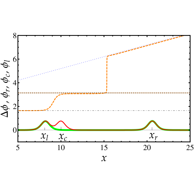
Figure 2: (Color online) The phase of solitons (dashed curves) and solitons intensity profiles (solid curves). Long dashed curve (orange) corresponds to the exact phase of the solitons calculated directly from the two solitons solution, Eq. (3). Dotted (blue) curve corresponds to the phase of the right soliton, $\phi_{r}$, calculated from Eq. (14). Thick dashed curve corresponds to the phase of the central soliton, $\phi_{c}$, calculated from Eq. (15). Dashed-dotted curve corresponds to the phase of the left soliton, $\phi_{l}$, calculated from Eq. (16). The solid curves correspond to the density profiles as in Fig. 1. The parameters used are: $\gamma(t)=0$, $n_{1}=1$, $n_{2}=1.01$, $x_{1}=10$, $x_{2}=20$, $v_{1}=1$, $v_{2}=1.2$, $g_{0}=3$, $\phi_{01}=\phi_{02}=0$, and $t=0$.

The above results are verified in Fig. 2, where we plot $\Delta\phi$, $\phi_{r}$, $\phi_{l}$, and $\phi_{c}$ versus $x$. The agreement between our estimated values and the exact curve is evident.

II.4 Soliton-soliton force

In this section, we use the results of the previous two subsections to derive the force between the left and right solitons. The force is proportional to the acceleration of the solitons separation

$$\Delta = x_{r}-x_{l}$$ (18)

$$= {x_{d}}(t)+\alpha e^{-\gamma(t)}$$

$$+ \left[{\beta_{1}}\cos({z_{r}}(t))e^{\frac{1}{4}g_{0}{n_{d}}{x_{d}}(t)e^{\gamma(t)}-\gamma(t)+2\gamma_{0}}\right.$$

$$+ {\beta_{2}}\cos({z_{l}}(t))e^{-\frac{1}{4}g_{0}{n_{d}}{x_{d}}(t)e^{\gamma(t)}-\gamma(t)}$$

$$+ {\beta_{3}}\sin({z_{l}}(t))e^{-\frac{1}{4}g_{0}{n_{d}}{x_{d}}(t)e^{\gamma(t)}-\gamma(t)-\gamma_{0}}$$

$$+ \left.{\beta_{4}}\sin({z_{r}}(t))e^{\frac{1}{4}g_{0}{n_{d}}{x_{d}}(t)e^{\gamma(t)}-\gamma(t)+\gamma_{0}}\right]\,e^{-\frac{1}{4}g_{0}{n_{s}}{x_{d}}(t)e^{\gamma(t)}},$$

where

$$\alpha=\frac{2(({n_{s}}-{n_{d}})\log({Y_{r}})+({n_{d}}+{n_{s}})\log({Y_{+}}))}{g_{0}\left({n_{d}}^{2}-{n_{s}}^{2}\right)},$$ (19)

and the coefficients $\beta_{1-4}$ are given in Appendix B.2. The first two terms on the right hand side of Eq. (18) are the dominant ones since they correspond to the noninteracting solitons separation, $x_{d}(t)$, and their logarithmic shifts $\propto\alpha$ arising from the interaction between solitons. The time-dependence of $\Delta$ originates from $\gamma(t)$, $z_{r,l}(t)$, and $x_{d}(t)$. The acceleration can thus be derived

$${\ddot{\Delta}}(t)=\left({\dot{\gamma}}(t)^{2}-{\ddot{\gamma}}(t)\right)\,\Delta(t)+\frac{1}{64}\,\left[{\beta_{5}}\sin({z_{l}}(t))+{\beta_{6}}\sin({z_{r}}(t))+{\beta_{7}}\cos({z_{l}}(t))+{\beta_{8}}\cos({z_{r}}(t))\right]\,e^{-\frac{1}{4}g_{0}n_{s}{\Delta}(t)e^{\gamma(t)}+3\gamma(t)},$$ (20)

where the coefficients $\beta_{5-8}$ are given in Appendix B.2. In the last equation, we have used Eq. (18) with only the first two terms of its right hand side to substitute for $x_{d}(t)$ in terms of $\Delta(t)$ in the exponential factor. The first term on the right hand side of Eq. (20) corresponds to the force due to the external potential which vanishes for the homogeneous case. The rest of the terms correspond to the force of interaction between the solitons. The interaction force depends, as expected, on the phase difference of the two solitons and decays exponentially with their separation. It should be noted that this equation is a generalization of Gordon’s formula gordon in two aspects. First, it is derived for a time-dependent inhomogeneous medium. Secondly we have, essentially, no restriction on the difference between the two solitons amplitudes and speeds; apart from some extreme cases which were mentioned in Appendix B.1 and will be discussed further below.

II.4.1 Gordon’s formula

For the homogeneous case, $\gamma(t)=0$, and in the limits $n_{d}\rightarrow 0$ and $\eta_{d}\rightarrow 0$, the acceleration formula, Eq. (20), simplifies considerably. An apparent inconsistency occurs when switching the order of these two limits, namely

$$\lim_{n_{d}\rightarrow 0}\,\lim_{\eta_{d}\rightarrow 0}\,{\ddot{\Delta}}(t)=-{1\over 8}\,(n_{s}\,g_{0})^{3}\,e^{-{1\over 4}n_{s}\,g_{0}\,\Delta}\,\cos{z},$$ (21)

while

$$\lim_{\eta_{d}\rightarrow 0}\,\lim_{n_{d}\rightarrow 0}\,{\ddot{\Delta}}(t)={1\over 8}\,(n_{s}\,g_{0})^{3}\,e^{-{1\over 4}n_{s}\,g_{0}\,\Delta}\,\cos{z},$$ (22)

which differ by an overall minus sign. The conflict is resolved by invoking Eq. (17) where it is shown that in the first case: $z=\Delta\phi$, while in the second case: $z=\pi-\Delta\phi$. Therefore, the two approaches agree on the following result

$${\ddot{\Delta}}(t)=-{1\over 8}\,(n_{s}\,g_{0})^{3}\,e^{-{1\over 4}n_{s}\,g_{0}\,\Delta}\,\cos{\Delta\phi}.$$ (23)

This is essentially Gordon’s result, Eq. (1), since in his derivation Gordon took $g_{0}=1$ and soliton amplitude $n_{j}\sqrt{g_{0}}/2=1$, $j=1,2$, as can be seen in Eqs.(1) and (6) of Ref. gordon . Substituting $g_{0}=1$ and $n_{s}=4$ in the last equation, it becomes identical to Eq. (1). It should be mentioned here that Eq. (1) was also derived in Ref. solov using a perturbation analysis based on the Inverse Scattering method, and in Ref. anderson using a variational calculation.

II.4.2 Our formula

For nonzero $\gamma(t)$ and in the limits $n_{d}\rightarrow 0$ and $\eta_{d}\rightarrow 0$, the acceleration formula takes the form

$${\ddot{\Delta}}(t)=\left({\dot{\gamma}}(t)^{2}-{\ddot{\gamma}}(t)\right)\,\Delta(t)-\frac{1}{16}\,(g_{0}\,n_{s})^{3}\,e^{-\frac{1}{4}g_{0}n_{s}\Delta(t)\,e^{\gamma(t)}+3\gamma(t)-\gamma_{0}}\,(1+e^{\gamma_{0}})\,\cos({\Delta\phi}).$$ (24)

This is a generalization to Gordon’s formula for the inhomogeneous case as modeled by Eq. (2). Depending on the specific form of $\gamma(t)$, the two force terms, namely the external (first term) and the interaction (second term), can be repulsive, attractive, or oscillatory. In addition, the phase difference $\Delta\phi(t)$ also depends on $\gamma(t)$. It is established in the homogeneous case, as will also be shown in section III, that the time-dependence of the phase difference is responsible for binding the two solitons in the soliton molecule. Here, in addition to the possibility of forming soliton molecules, the dependence of $\Delta\phi(t)$ on $\gamma(t)$ allows for controlling the parameters of the molecule such as its equilibrium bond length, period, and spring constant. This and possibly other interesting phenomena will be left for future investigation.

II.4.3 Comparison with numerical calculations

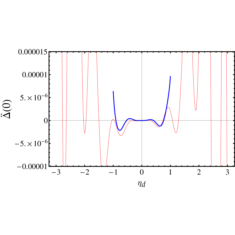
Figure 3: (Color online) The initial acceleration of the solitons separation, ${\ddot{\Delta}}(0)$, versus $\eta_{d}$. Thick (blue) curve is calculated from Eq. (20). Light (red) curve is calculated numerically from the exact two solitons solution, Eq. (3). The parameters used are: $\gamma(t)=0$, $n_{1}=1$, $n_{2}=1.01$, $x_{1}=10$, $x_{2}=20$, $v_{1}=1$, $g_{0}=3$, $\phi_{01}=\phi_{02}=0$, and $t=0$.

To obtain an estimate of the accuracy of the general acceleration formula, Eq. (20), we calculate numerically the acceleration from the exact two solitons solution, Eq. (3), and compare the two results. The distance between the two solitons of the function $|\Psi(x,t)|^{2}$ is determined using a numerical algorithm that employs our formulae for $x_{l}$ and $x_{r}$ given by Eqs. (4) and (6) to calculate seed values. The distance is then differentiated numerically twice at $t=0$. In Fig. 3, we compare the two results. Good agreement is obtained for $|\eta_{d}|\lesssim 1$. The analytical solution diverges at $\eta_{d}\thickapprox\pm 1$. The value at which divergence takes place is set by the specific choice of parameters in Fig. 3. As pointed out in section II.2, the divergence occurs due to the merging of the central and left solitons. This artifact divergency can be remedied by associating the location of the local maximum of $q$ to $x_{l}$ once this maximum has reached the $x$-axis from above.

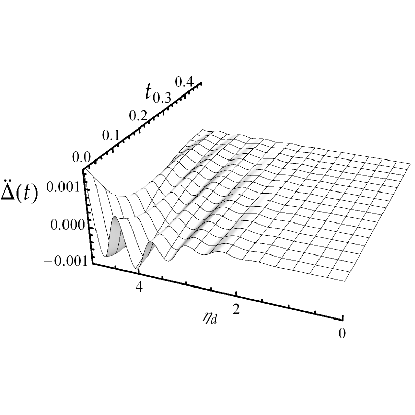
Figure 4: The acceleration of the solitons separation, ${\ddot{\Delta}}(0)$, versus $\eta_{d}$ and $t$. The parameters used are: $\gamma(t)=0$, $n_{1}=1$, $n_{2}=1.01$, $x_{1}=10$, $x_{2}=20$, $v_{1}=1$, $g_{0}=3$, $\phi_{01}=\phi_{02}=0$.

Restricting our study to the region where agreement is obtained, we interestingly notice that the acceleration is oscillating between positive and negative values. This means that the force between the solitons is oscillating between attractive and repulsive. The possibility of having attractive forces for finite $\eta_{d}$ is particularly interesting; for two solitons with nonzero relative positive speed, i.e. the solitons are initially diverging from each other, the force between them is attractive. This suggests that, if the force remains attractive for sufficient time, the two solitons will slow down and eventually converge at some point. If true, this should occur at small distances since the force decays exponentially with distance and when the two solitons are allowed to diverge even for a short while, the force might be weakened such that the two solitons can not return back. To be able to judge on such a possibility, we need to know what happens to the acceleration at later times. To that end, we calculate numerically the acceleration in terms of $\eta_{d}$ and $t$. The result is plotted in Fig. 4, where it is clear that the acceleration indeed decays with time for all $\eta_{d}$. This leads to that any nontrivial effect of the oscillating force is most likely to take place at short solitons separations. This is what we find in the next section where the possibility of forming stable soliton molecules is pointed out.

III Soliton molecule

We have shown in the previous section that, as a result of the solitons time-dependent relative phase, the force of interaction between solitons is oscillating between repulsive and attractive. Since the force decays exponentially with the solitons separations, this oscillation will have a tangible effect only when the two solitons are close to each other. In this section, we investigate the force of interaction between solitons for short solitons separation. In such a special case, Eq. (18) takes a simple form that accounts for the solitons separation in terms of their relative phase. Using this formula, we show that the solitons will be bound to oscillate around some equilibrium distance where the phase plays the role of the restoring force. Comparison with exact numerical calculations shows that this formula is accurate for almost the full range of the solitons separation, except at the coalescence point (if any). In subsection III.1, we discuss the main features of the resulting soliton molecules, and in subsection III.2, we investigate numerically their stability in different scattering regimes.

To focus on the role of relative phase, we simplify the analysis by restricting our treatment to the homogeneous case, $\gamma(t)=0$, and zero relative speed, $\eta_{d}=v_{d}=v_{2}-v_{1}=0$. We also set $x_{1}=x_{2}$ so that any separation between the solitons to be as small as possible which in this case arises only from the logarithmic shifts ($\sim\alpha$ in Eq. (18)). In this case, the solitons separation $\Delta$, given by Eq. (18), simplifies in the limit $n_{d}\ll n_{s}$ to

$$\Delta(t)=\frac{4}{g_{0}n_{s}}\log\left[1+2\,n_{s}\,g_{0}\,\cos{\left(\frac{1}{8}\,g_{0}^{2}\,n_{d}\,n_{s}\,t\right)+(n_{s}\,g_{0})^{2}}\right]-\frac{4}{g_{0}n_{s}}\log\left(\frac{g_{0}n_{d}^{2}}{n_{s}}\right),$$ (25)

and the acceleration is given by

$${\ddot{\Delta}}(t)=-{1\over 8}\,(n_{s}\,g_{0})^{3}\,\frac{2\,n_{s}\,g_{0}+(n_{s}\,g_{0})^{2}\,\cos\left(\frac{1}{8}\,g_{0}^{2}\,n_{d}\,n_{s}\,t\right)+\cos\left(\frac{1}{8}\,g_{0}^{2}\,n_{d}\,n_{s}\,t\right)}{1+2\,n_{s}\,g_{0}\,\cos\left(\frac{1}{8}\,g_{0}^{2}\,n_{d}\,n_{s}\,t\right)+(n_{s}\,g_{0})^{2}}\,e^{-\frac{1}{4}g_{0}n_{s}{\Delta\,x}}.$$ (26)

It is noted that for $n_{s}\,g_{0}\gg 1$ or $n_{s}\,g_{0}\ll 1$, Gordon’s formula is retrieved, but here with an explicit time-dependence of the phase, $\Delta\phi=n_{d}\,n_{s}\,g_{0}\,t/8$. This acceleration formula deviates considerably from Gordon’s formula for $n_{s}\,g_{0}\sim 1$. Specifically, for $n_{s}\,g_{0}=1$, $\Delta$ diverges to $-\infty$ at $\cos{(n_{d}\,n_{s}\,g_{0}\,t/8)}=-1$, which indicates that the two solitons coalesce. This is confirmed below by examining the exact solution at this condition. We note here that an approximate expression for the solitons separation was also derived in Refs. solov ; anderson ; desem . In addition, our predicted molecule’s oscillation frequency (see Eq. (33) below) agrees with these references.

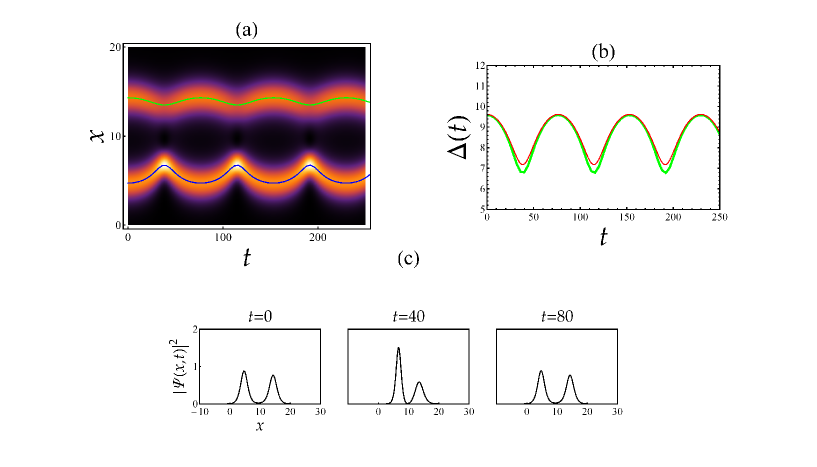
Figure 5: (Color online) Density profile of the soliton molecule and the solitons center-of-mass trajectories and separations. (a) Density plot corresponds to solitons density. Curves correspond to solitons trajectories calculated numerically from the exact solution (3). (b) Thick (green) curve is solitons separation calculated from the exact solution (3). Light (red) curve is the solitons separation calculated from formula (25). (c) Density profile at some specific times. The parameters used are: $\gamma(t)=0$, $n_{1}=2.37$, $n_{d}=0.5$, $x_{1}=x_{2}=10$, $v_{1}=v_{2}=0$, $g_{0}=0.5$, $\phi_{01}=\phi_{02}=0$.

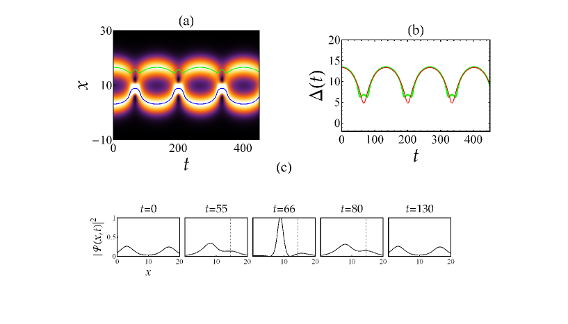
Figure 6: Same as Fig. 5 but with $n_{1}=1.25$.

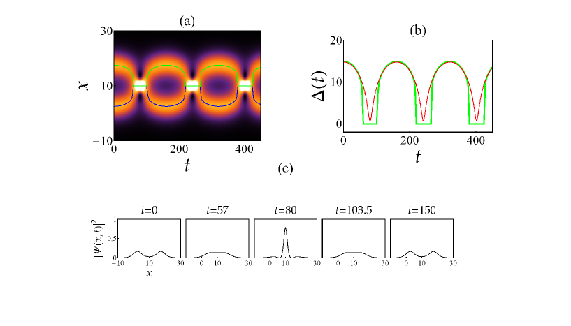
Figure 7: Same as Fig. 5 but with $n_{1}=1$.

To verify this feature, we calculate numerically the distance between the two solitons directly from the exact solution, Eq. (3), for different values of $n_{s}\,g_{0}$. For $n_{s}\,g_{0}=2.5$, the density plot in Fig. 5a, shows a soliton molecule of two clearly resolved solitons with a separation oscillating around some nonzero equilibrium distance. Approaching the solitons coalescence point with $n_{s}\,g_{0}=1.5$, the density plot in Fig. 6a, shows the two solitons approaching each other more than the previous case. Furthermore, this figure shows a slight bounce back by one of the solitons in the region of collision. Approaching further the coalescence condition with $n_{s}\,g_{0}=1.25$, we indeed observe in Fig. 7a that the two solitons merge almost completely. For a more quantitative comparison, we calculate numerically the center-of-mass trajectories of the two solitons. We show the trajectory curves in the density plots of Figs. 5a-7a. In Figs. 5b-7b, we plot the solitons separation obtained from formula (25) and the numerical trajectories obtained from the exact solution. It is clear from these figures that this formula agrees well with the exact soliton separation except near the collision region. In Fig. 5b, the two solitons remain away from each other during the collision, and therefore good agreement is obtained with the exact result even in the collision region. In Fig. 6b the two solitons approach each other further such that formula (25) does not account for the above-mentioned slight bounce of one of the solitons. In Fig. 7b, agreement with the exact solution in the collision region is qualitative. We found that at the condition $n_{s}\,g_{0}=1$ and for $n_{d}\ll n_{s}$, the analytic curve overlaps with that of the exact solution; apart from the horizontal segments where formula (25) diverges to $-\infty$. Further insight is obtained by plotting the density profile of the soliton molecule at some specific times, as shown in Figs. 5c-7c. In Fig. 5c, we observe that the initial amplitude imbalance is never removed during the dynamics. Instead, it becomes maximum when the two solitons are closest to each other. In addition, we notice that the oscillation amplitude of the larger soliton around its equilibrium position is larger. Figure 6c shows clearly the soliton bounce which takes place in the time interval $t=55$ to $t=80$. In these subfigures we plot two vertical dashed lines that indicate the position of the solitons at the closest approach. It is clear that after first closest approach at $t=55$, the right soliton bounces back with a maximum displacement at $t=66$. In Fig. 7c, it is shown that, although the two solitons coalesce, two small symmetric $\it wings$ appear. A detailed examination of these wings shows that they are the remnants of the two solitons after they coalesce and they both bounce back in the collision region similar to the case of Fig. 6.

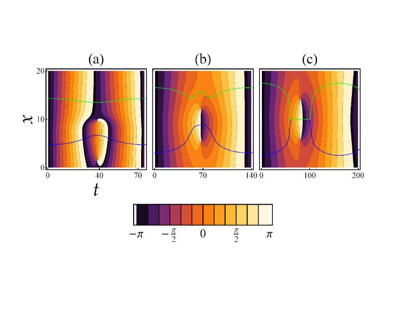
Figure 8: Contour plots showing the phase of the soliton molecules of Figs. 5-7. Subfigures (a), (b), and (c), correspond to Fig. 5, Fig. 6, and Fig. 7, respectively. The blue (lower) and green (upper) curves correspond to the center-of-mass trajectories of the left and right solitons, respectively.

It is also instructive to show the dynamics of the phase profile during the molecule’s oscillation. This is shown with the contour plots of Fig. 8 which correspond to the molecules of Figs. 5-7. In Fig. 8a, which corresponds to Fig. 5, the two solitons start initially in phase. By time the phase of the right soliton, which is the one with higher intensity amplitude and larger oscillation displacement, starts to exceed that of the left soliton. At the point of closest approach, the phase difference is exactly $\pi$. After that point, the two solitons diverge again, the phase difference starts to decrease, and the cycle is repeated. Similar behavior is seen in Fig. 8b. However, in Fig. 8c, where the two solitons coalesce for a considerable amount of time, the phase difference during the coalescence time is zero. It is thus not completely understood why, in this case, the two solitons still repel each other and eventually split.

III.1 Molecule formation and dynamics

Having established the existence of the soliton molecule from the exact two solitons solution and derived a formula that describes its bond length, here we use this formula to examine more closely the propertie of the soliton molecule and its mechanism of binding.

It is clear from Eq. (26) that the sinusoidal time-dependence of the solitons relative phase leads to a force of interaction that oscillates between attractive and repulsive and hence allowing for soliton molecule formation. Further details of the mechanism of binding will be uncovered by expressing the acceleration, ${\ddot{\Delta}}(t)$ in terms of $\Delta(t)$ by substituting for $\cos{(n_{s}\,n_{d}\,g_{0}^{2}\,t/8)}$ from Eq. (25) into Eq. (26), to get

$${\ddot{\Delta}}=\frac{1}{16}g_{0}n_{s}\left(1-g_{0}^{2}n_{s}^{2}\right){}^{2}\left(\frac{n_{s}}{n_{d}}\right)^{2}e^{-\frac{1}{2}g_{0}n_{s}{\Delta}}-\frac{1}{16}\left(g_{0}n_{s}\right){}^{2}\left(g_{0}^{2}n_{s}^{2}+1\right)e^{-\frac{1}{4}g_{0}n_{s}{\Delta}}.$$ (27)

This shows that the interaction force between the two solitons is the resultant of an attractive part and a repulsive part. The equilibrium bond length, defined by ${\ddot{\Delta}}(\Delta=\Delta_{\rm eq})=0$, is given by

$${\Delta_{\rm eq}}=\frac{4}{g_{0}n_{s}}\log\left(\frac{n_{s}\left(g_{0}^{2}n_{s}^{2}-1\right){}^{2}}{{n_{d}^{2}}\,g_{0}\left(g_{0}^{2}n_{s}^{2}+1\right)}\right).$$ (28)

In consistence with our previous result, the equilibrium bond length diverges as $-\log{n_{d}}$. Solving the last equation for $n_{d}^{2}$ and then substituting in Eq. (27), ${\ddot{\Delta}}$ simplifies to

$${\ddot{\Delta}}=\frac{1}{16}g_{0}^{2}n_{s}^{2}\left(g_{0}^{2}n_{s}^{2}+1\right)\left[\left(e^{-\frac{1}{4}g_{0}n_{s}\left({\Delta}-\frac{{\Delta_{\rm eq}}}{2}\right)}\right){}^{2}-e^{-\frac{1}{4}g_{0}n_{s}{\Delta}}\right].$$ (29)

For small amplitude oscillations, $\Delta\simeq\Delta_{\rm eq}$, the last equation gives

$${\ddot{\Delta}}=-\frac{1}{64}g_{0}^{3}n_{s}^{3}\left(g_{0}^{2}n_{s}^{2}+1\right)({\Delta}-\Delta_{\rm eq})e^{-\frac{1}{4}g_{0}n_{s}{\Delta_{\rm eq}}}.$$ (30)

The restoring force ($\sim\Delta$) originates from the phase-dependent terms, $\cos{(n_{d}\,n_{s}\,g_{0}^{2}\,t/8)}$. This appealing form of the force of interaction shows that the force between the solitons is of Hooke’s law type with a spring constant

$$k=\frac{m}{64}g_{0}^{3}n_{s}^{3}\left(g_{0}^{2}n_{s}^{2}+1\right)e^{-\frac{1}{4}g_{0}n_{s}{\Delta_{\rm eq}}},$$ (31)

where $m$ is the bare mass of the molecule. Expressed in terms of $n_{s}$ and $n_{d}$, the spring constant takes the form

$$k=\frac{g_{0}^{4}n_{d}^{2}n_{s}^{2}\left(g_{0}^{2}n_{s}^{2}+1\right){}^{2}}{64\left(g_{0}^{2}n_{s}^{2}-1\right)^{2}}\,m,$$ (32)

which shows that $k=0$ for $n_{d}=0$; corresponding to a soliton molecule of infinite bond length. Furthermore, $k$ diverges for $n_{s}\,g_{0}=1$, which signifies soliton coalescence, as we have pointed out in the previous subsection. Since the frequency of the soliton molecule is given by

$$\omega={1\over 8}\,n_{d}\,n_{s}\,g_{0}^{2},$$ (33)

and the spring constant is given in Eq. (32), the effective mass $m^{*}=k/\omega^{2}$ will be given by

$$m^{*}=\frac{\left(g_{0}^{2}n_{s}^{2}+1\right){}^{2}}{\left(g_{0}^{2}n_{s}^{2}-1\right)^{2}}\,m,$$ (34)

which again diverges at the soliton coalescence condition, $n_{s}\,g_{0}=1$. Having determined the main properties of the soliton molecule, we can now return back to Eq. (25) to express $\Delta$ as

$${\Delta}={\Delta_{0}}+\frac{4}{g_{0}n_{s}}\log\left(\frac{g_{0}^{2}n_{s}^{2}+2g_{0}n_{s}\cos(\omega\,t)+1}{\left(g_{0}n_{s}+1\right){}^{2}}\right),$$ (35)

where $\Delta_{0}$ is the initial value of $\Delta$, which is given by the solitons parameters through

$${\Delta_{0}}={\Delta_{\rm eq}}+\frac{4}{g_{0}\,n_{s}}\,\log\left(\frac{1+g_{0}^{2}{n_{s}}^{2}}{\left(1-g_{0}{n_{s}}\right)^{2}}\right).$$ (36)

The amplitude of the oscillation $\Delta_{\rm max}=\Delta_{0}-\Delta_{\rm eq}$ is thus given by

$$\Delta_{\rm max}=\frac{4}{g_{0}\,n_{s}}\,\log\left(\frac{1+g_{0}^{2}{n_{s}}^{2}}{\left(1-g_{0}{n_{s}}\right)^{2}}\right),$$ (37)

which gives an elastic potential energy

$$E={1\over 2}\,k\,\Delta_{\rm max}^{2}={1\over 8}\,g_{0}^{2}\,n_{d}^{2}\,{\left(1+g_{0}^{2}{n_{s}}^{2}\over{1-g_{0}^{2}{n_{s}}^{2}}\right)^{2}}\,{\log^{2}\left(\frac{1+g_{0}^{2}{n_{s}}^{2}}{\left(1-g_{0}{n_{s}}\right)^{2}}\right)}.$$ (38)

It should be noted here that this is equal to the mechanical energy since the initial speed vanishes, ${\dot{\Delta}}(0)=0$. The fact that the potential energy diverges at the coalescence condition $n_{s}\,g_{0}=1$ is a gain an artifact of the calculation, but it at least indicates that the bond is tighter than cases where $n_{s}\,g_{0}\gg 1$ or $n_{s}\,g_{0}\ll 1$.

III.2 Stability

Here, we investigate the stability of the soliton molecule against break up in the following three collision regimes: $i)$ reflection by a hard wall, $ii)$ crossing a finite potential barrier, and $iii)$ collision with a single soliton. To that end we solve the Gross-Pitaevskii equation, Eq. (2), numerically. As an initial state, we use, for cases $i)$ and $ii)$ the two solitons solution, Eq. (3), which represents the soliton molecule. For case $iii)$, we use the superposition of the exact single soliton, Eq. (44), with the two solitons solution.

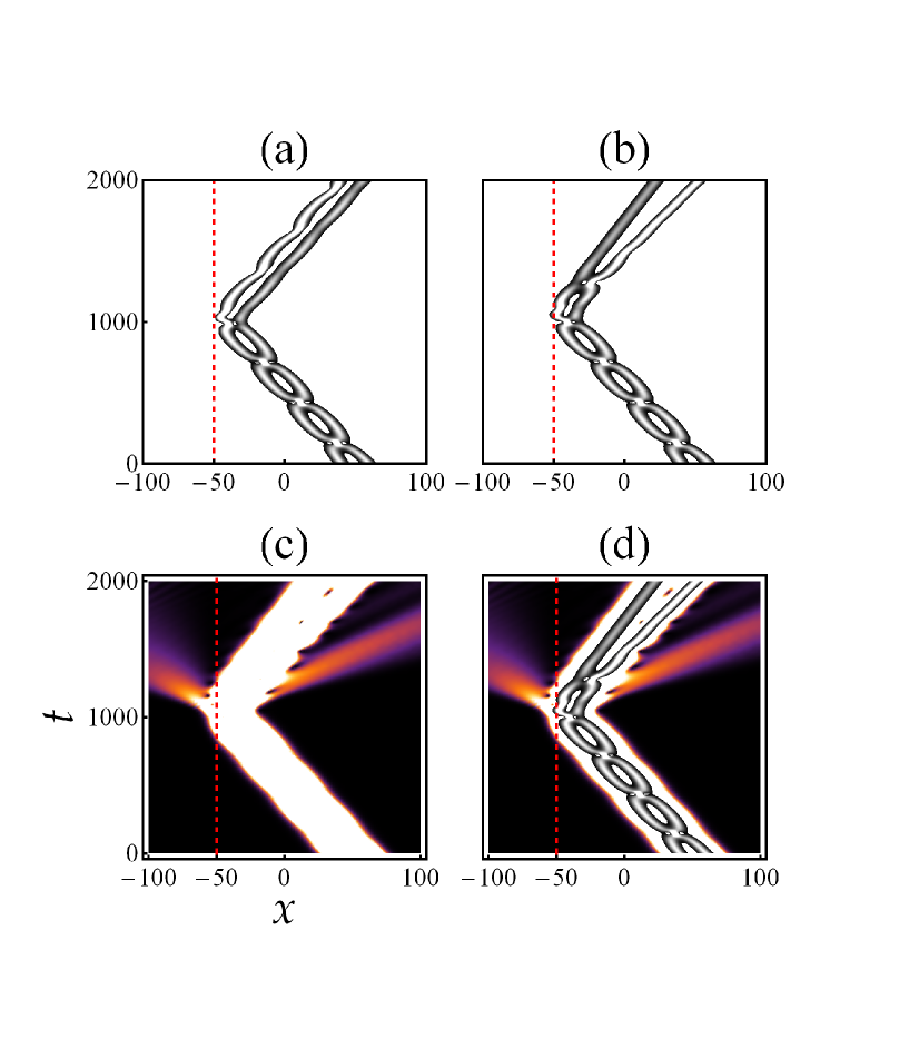
Figure 9: Soliton molecule reflection by a potential step given by Eq. (39). The dashed vertical line represents the interface of the potential step. The parameters used are: $g_{0}=0.5$, $x_{2}=x_{1}=50$, $\phi_{01}=\phi_{02}=c=0$, $n_{d}=0.3$, $n_{1}=1.0$, $\eta=-0.1$, $x_{0}=-50$. (a) $V_{0}=100$. (b),(c),(d) $V_{0}=0.075$.

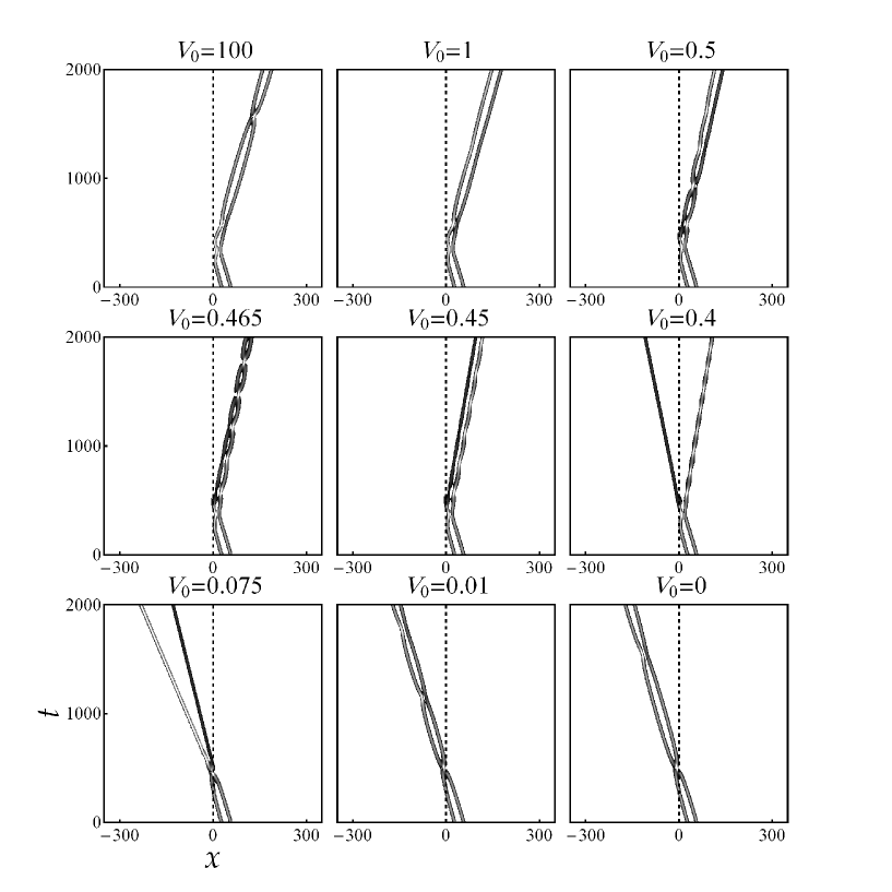
Figure 10: Soliton molecule reflection by and transmitting through a potential barrier given by Eq. (40) for different barrier heights. The parameters used are: $g_{0}=0.5$, $x_{2}=x_{1}=42$, $\phi_{01}=\phi_{02}=c=0$, $n_{d}=0.1$, $n_{1}=0.95$, $\eta=-0.1$, $d=0.005$, $x_{0}=0$.

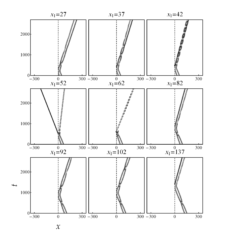
Figure 11: Soliton molecule reflection by a potential barrier given by Eq. (40) for different initial positions of the molecule. The parameters used are: $x_{2}=x_{1}$, $g_{0}=0.5$, $\phi_{01}=\phi_{02}=c=0$, $n_{d}=0.1$, $n_{1}=0.95$, $\eta=-0.1$, $V_{0}=0.465$, $d=0.005$, $x_{0}=0$.

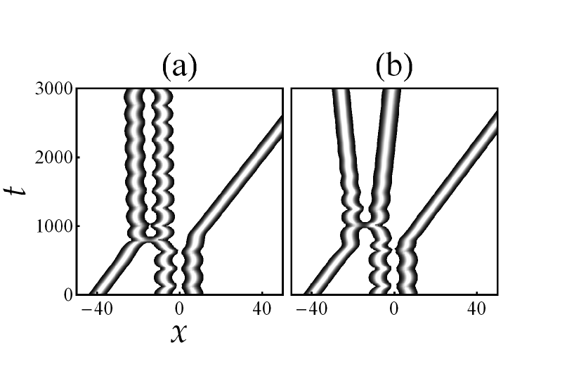
Figure 12: Collision between a single soliton and a soliton molecule for two single soliton phases. $g_{0}=0.5$, $x_{2}=x_{1}=\phi_{01}=\phi_{02}=c=0$, $n_{d}=0.2$, $n_{1}=1.9$, $n_{3}=2$, $x_{3}=-40$, $\eta_{3}=0.025$. The phase difference between the injected soliton of (b) and that of (a) equals $\pi$.

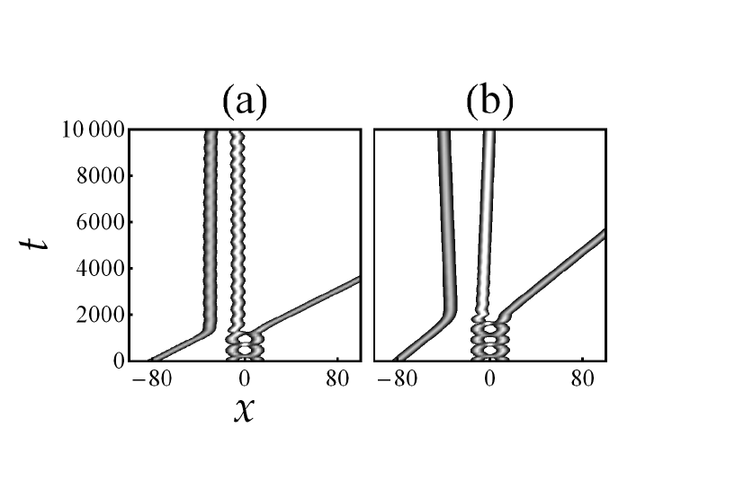
Figure 13: Collision between a single soliton and a soliton molecule for two single soliton initial speeds. $g_{0}=0.5$, $x_{2}=x_{1}=\phi_{01}=\phi_{02}=c=0$, $n_{d}=0.2$, $n_{1}=1$, $n_{3}=1$, $x_{3}=-80$. (a) $\eta_{3}=-0.04$, (b) $\eta_{3}=-0.025$.

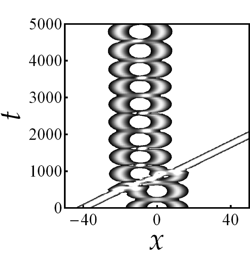
Figure 14: Collision between a high intensity single soliton and a soliton molecule. $g_{0}=0.5$, $x_{2}=x_{1}=\phi_{01}=\phi_{02}=c=0$, $n_{d}=0.2$, $n_{1}=1$, $n_{3}=2$, $\eta_{3}=0.04$, $x_{3}=-40$.

Before starting the discussion of results, we point out that in Figs. 9-14, we present the results of this section using spacio-temporal density plots. Since the solitons are too thin compared to the spacial range that we consider, a density plot with full spacial and time ranges will not show a clear solitons peak density or center-of-mass path, as Fig. 9c shows. To solve this problem, we restricted the density plotting to a finite range of $|\Psi(x,t)|^{2}$, namely between 0.025 and 0.15 corresponding to the upper part of the solitons peaks. This results in an easier tracking of both the solitons peak density and center-of-mass path, as shown in Fig. 9a,b,d and the rest of subsequent figures.

For reflection from a hard wall we solve Eq. (2) with a potential step of the form

$$V(x)=\left\{\begin{array}[]{cc}V_{0}\,,&x<x_{0},\\ \\ 0\,,&x\geq x_{0},\end{array}\right.$$ (39)

where $V_{0}$ and $x_{0}$ are the hight and location of the potential wall, respectively. The result of reflection from this hard wall, with $V_{0}=100$, is shown in Fig. 9a. The soliton molecule preserves its molecular structure but with different characteristics. The solitons in the reflected molecule do not coalesce as in the incident molecule. In other words, the equilibrium bond length becomes larger. The density plot shows that initially the two solitons are of comparable intensities. After reflection, the brighter color of the left soliton and darker color of the right soliton indicate that the left soliton acquires higher intensity on the expense of the right soliton. We also notice that the left soliton performs two reflections from the potential interface. After the first reflection, it collides with the right soliton and then collides with the potential interface for the second time.

The picture becomes different when the hight of the wall is reduced to $V_{0}=0.075$, as shown in Fig. 9b. The soliton molecule breaks up after reflection. This is due to loss of energy at the interface of the potential. Part of the soliton molecule transmits as a nonsolitonic pulse that broadens and decays in intensity by time. By plotting $|\Psi(x,t)|^{2}$ in Fig. 9c with its full range, we can see the nonsolitonic part as the left- and right-going two red ejections corresponding to the transmitted and reflected nonsolitonic pulses, respectively. In Fig. 9d, we combine Fig. 9b and Fig. 9c to show the locations of the nonsolitonic ejections with respect to the solitons centers. In the case of reflection from a hard wall, the nonsolitonic ejections are essentially not present which results in the stability of the molecular structure.

For reflection from a potential barrier we solve Eq. (2) with the potential

$$V(x)=\left\{\begin{array}[]{cc}V_{0},&x_{0}-d<x<x_{0},\\ \\ 0&{\rm elsewhere},\end{array}\right.$$ (40)

where $V_{0}$, $d$, and $x_{0}$, are the height, width, and location of the right side of the barrier, respectively. In Fig. 10, we show the many different possibilities that result when the height of the barrier is changed. The free evolution case with $V_{0}=0$ is shown as a reference plot. The full reflection case is shown for $V_{0}=100$, which is similar to the previous case of reflection from a hard wall. Reducing the height of the barrier to $V_{0}=1$, we notice that the soliton molecule breaks up after reflection. As pointed above, this is due to the nonsolitonic ejections taking place at the interfaces of the potential. Reducing the height of the barrier to $V_{0}=0.5$, a sign of solitons recombining appears in the form of a soliton molecule of a short lifetime. At $V_{0}=0.465$ a stable molecule is remarkably formed with a considerably shorter period than for the incident molecule. We have confirmed numerically that this molecule remains stable for much longer time provided that the soliton molecule remains sufficiently far from the boundaries of the spacial grid. This unique structure remains for some small domain around $V_{0}=0.465$, but is lost for $V_{0}=0.45$, where the molecule breaks for long evolution times. Decreasing the height of the barrier to $V_{0}=0.4$, the molecule breaks at the interface and splits into a reflected and transmitted solitons. For $V_{0}=0.075$, the molecule breaks at the interface, but both solitons transmit through the barrier. For $V_{0}=0.01$, the transmitted solitons show a sign of recombining again but with shorter period than for the free evolution case and larger than in the case of $V_{0}=0.465$.

Motivated by the fact that at the coalescence point the intensity of the molecule is considerably higher than at other instants, we expect to find different scattering dynamics when the soliton molecule meets the interface of the potential at different phases of its periodic oscillation. In Fig. 11, this is investigated by fixing the height of the potential barrier at $V_{0}=0.465$ and changing the initial launching position of the molecule. Starting at $x_{1}=27$, the molecule breaks after reflection. A shortly-lived molecule is obtained at $x_{1}=37$, and a stable molecule is found for $x_{1}=42$, which corresponds to the $V_{0}=0.465$ case of Fig. 10. At $x_{1}=52$, the soliton splits at the interface into transmitted and reflected solitons. The coalescence point is, in this case, located at the interface. Transmission takes place due to the high intensity of the soliton at the coalescence point. At $x_{1}=62$, the two solitons still split as in the previous subfigure but with a weak transmitted soliton intensity less than 0.025 and hence will not be shown in our density plots which are restricted to the intensities between 0.025 and 0.15, as pointed out previously. For $x_{1}=82$, the coalescence point takes place before the molecule reaches the interface and both solitons reflect but the molecule breaks up. For $x_{1}=92$ the two reflected solitons start to recombine forming a stable molecule at $x_{1}=102$. At $x_{1}=137$ the reflected molecule starts to break up since the second coalescence point becomes close to the interface. Thus, the conclusion from this figure is that the soliton molecule is more vulnerable to break up when it meets the interface at the coalescence point. Equivalently, soliton molecules with larger equilibrium bond length, such that coalescence does not occur, will be more stable against breakup post reflection from barriers.

Finally, we present in Figs. 12-14 the results of scattering of a soliton molecule by a single soliton described by Eq. (43) with normalization $n_{3}$, center-of-mass position and speed $x_{3}$ and $\eta_{3}=v_{3}$, respectively. The effects of the phase, speed, and amplitude of the injected soliton are investigated separately. In Fig. 12a, a soliton initially at $x=-40$ is launched towards a stationary soliton molecule near $x=0$. At the impact, the molecule brakes up, its right soliton is ejected in the direction of the positive $x$-axis, and the left soliton combines with the scatterer soliton to form a new stationary molecule shifted by about a bond length to the left. We point out here that for such an outcome to occur, it is essential that the amplitude of the scatterer soliton is nearly equal to that of the right soliton of the molecule. Otherwise, a different outcome, as that of Fig. 14, will be obtained. In Fig. 12b, the same numerical experiment is repeated but with adding a $\pi$ to the phase of the scatterer soliton. Clearly, this phase addition prevents the formation of a new molecule resulting in three solitons diverging from each other. From applications point of view, the phase of $\pi$ could be used as a “key” to “unlock” the molecule for the purpose of extracting stored data. In Fig. 13, we show the effect of the initial speed of the injected soliton. In contrary to one’s first judgment, the molecule preserves its structure for fast collisions, as in Fig. 13a, and breaks up for slower collisions, as in Fig. 13b. In Fig. 14, the injected soliton has an amplitude that is approximately two times larger than any of the two solitons of the molecule. The injected soliton penetrates the molecule leaving it almost unchanged apart from a center-of-mass shift to the left.

IV Conclusions

We have used the Inverse Scattering method to derive the two solitons solution of a nonlinear Schr$\rm\ddot{o}$diner equation with a parabolic potential and cubic nonlinearity with time-dependent coefficients, as given by Eq. (2). The solution was then simplified and put in a suggestive form in terms of the fundamental parameters of the two solitons, namely their amplitudes, center-of-mass positions and speeds, and their phases. In this form, two different regimes of the solution, namely the resolved solitons and overlapping solitons, were distinguished and the main features such as the solitons separation and relative phase were extracted. From the expression for the solitons separation we find that for the homogeneous case and zero solitons relative speed, the solitons separation diverges logarithmically with the solitons amplitude difference such that, for equal solitons, the trivial solution is obtained.

The force of interaction was then derived, essentially, for arbitrary solitons parameters. This resulted in generalizing Gordon’s formula gordon to i) the generalized inhomogeneous case considered here, ii) arbitrary solitons relative speed and amplitudes, and iii) short solitons separations (compared to their width). With this formula, the possibility of forming soliton molecules emerged naturally, where the force at short distance was shown to be composed of an attractive part, resulting from the nonlinearity, and another part that oscillates between repulsive and attractive resulting from the time-dependent relative phase. The main features of the soliton molecule, including its equilibrium bond length and bond spring constant, frequency and amplitude of oscillation, effective mass, and its elastic potential energy, where then calculated in terms of the solitons parameters. It turns out that the amplitudes difference $n_{d}=n_{2}-n_{1}$ plays an important role in determining these quantities. Furthermore, we show that at the condition $g_{0}\,n_{s}=1$, the two solitons coalesce while away from this condition, the solitons approach each other but remain resolved. At this condition, the molecule’s effective mass and spring constant have maximum values. In our expressions Eqs. (32) and (34) diverge because these formulae were derived assuming the solitons remain resolved.

To have a sense of its stability we investigated numerically i) the collision of the soliton molecule with a hard wall and softer one, ii) scattering by a potential barrier, and iii) collision with a single molecule. The first case showed that while the molecular structure is preserved after reflection from a hard wall, it breaks when reflecting from a softer one. Reflection from a finite barrier showed that the molecular structure is preserved only for specific heights of the barrier. For an incident molecule with the coalescence condition satisfied, the molecule will be most vulnerable to break up when the coalescence point takes place at the interface of the barrier. This is simply understood by the fact that the intensity of the soliton molecule is maximum when the two solitons coalesce such that tunneling becomes possible. Stability of the molecule was also investigated by scattering the molecule with a single soliton. It turned that slower collisions tend to break up the molecule more easily than faster ones. In addition, the outcome of the collision depends on the phase of the incoming soliton such that a scatterer soliton which is in-phase with the molecule will typically preserve its molecular structure, but for an out-of-phase soliton, the molecule breaks up.

The two solitons solution presented here and the analysis that shows how to extract the solitons separation and relative phase may constitute the basis for a more accurate and detailed investigation of the origin of the soliton-soliton force, especially for short separations and at coalescence. The results of this paper will be hopefully of relevance to possible future applications of soliton molecules as data carriers or memories.

Appendix A Deriving the two solitons solution

The Lax pair associated with the Gross-Pitaevskii equation, Eq. (2), is obtained using our Lax pair search method usama_lax ; usama_vib and reads

$${\bf\Phi}_{x}=\zeta\,{\bf J}\cdot{\bf\Phi}\cdot{\bf\Lambda}+{\bf P}\cdot{\bf\Phi},$$ (41)

$${\bf\Phi}_{t}=i\,\zeta^{2}\,{\bf J}\cdot{\bf\Phi}\cdot{\bf\Lambda}\cdot{\bf\Lambda}+\zeta\,\left(i\,{\bf P}+x\,{\dot{\gamma}}\,{\bf J}\right)\cdot{\bf\Phi}\cdot{\bf\Lambda}+{\bf W}\cdot{\bf\Phi},$$ (42)

where

${\bf\Phi}(x,t)=\left(\begin{array}[]{cc}\psi_{1}(x,t)&\psi_{2}(x,t)\\ \phi_{1}(x,t)&\phi_{2}(x,t)\end{array}\right)$,     ${\bf\Lambda}=\left(\begin{array}[]{cc}\lambda_{1}&0\\ 0&\lambda_{2}\end{array}\right)$,     ${\bf J}=\left(\begin{array}[]{cc}1&0\\ 0&-1\end{array}\right)$,     ${\bf P}=\left(\begin{array}[]{cc}0&\sqrt{g_{0}}\,Q\\ -\sqrt{g_{0}}\,Q^{*}&0\end{array}\right)$,


${\bf W}=\left(\begin{array}[]{cc}i\,g_{0}\,|Q|^{2}/2&\sqrt{g_{0}}\,x\,{\dot{\gamma}}\,Q+i\,\sqrt{g_{0}}\,Q_{x}/2\\ -\sqrt{g_{0}}\,x\,{\dot{\gamma}}\,Q^{*}+i\,\sqrt{g_{0}}\,Q^{*}_{x}/2&-i\,g_{0}\,|Q|^{2}/2\end{array}\right)$,


$\zeta(t)=\sqrt{2}\,e^{\gamma(t)}$, $Q(x,t)=\Psi(x,t)\,e^{(\gamma(t)+i\,{\dot{\gamma}}(t)\,x^{2})/2}$, and $\lambda_{1}$ and $\lambda_{2}$ are arbitrary constants. Here, $\Psi(x,t)$ is the solution of Eq. (2) and ${\bf\Phi}$ is the auxiliary field.

The compatibility condition ${\bf\Phi}_{xt}={\bf\Phi}_{tx}$ of the linear system, Eqs. (41) and (42), is equivalent to the Gross-Pitaevskii equation, Eq. (2), and its complex conjugate. For a known seed solution, $\Psi_{0}(x,t)$, of Eq. (2) the linear system will have the solution ${\bf\Phi_{0}}$. The Darboux transformation is defined as ${\bf\Phi}[1]={\bf\Phi}\cdot{\Lambda}-{\bf\sigma}\,{\bf\Phi}$, where ${\bf\Phi}[1]$ is the transformed field and ${\bf\sigma}={\bf\Phi_{0}}\cdot{\bf\Lambda}\cdot{\bf\Phi_{0}}^{-1}$. Requiring the linear system to be covariant under the Darboux transformation imposes the transformation ${\bf P}[1]={\bf P}+{\bf J}\cdot{\bf\sigma}-{\bf\sigma}\cdot{\bf J}$, where ${\bf P}[1]$ is the transformed ${\bf P}$. This gives the new solution in terms of the seed solution as

$$\Psi(x,t)=\Psi_{0}(x,t)-\sqrt{8\over g_{0}}\,(\lambda_{1}-\lambda_{2})\,e^{(\gamma(t)-i\,{\dot{\gamma}}(t)\,x^{2})/2}{\psi_{1}(x,t)\,\psi_{2}(x,t)\over\phi_{2}(x,t)\,\psi_{1}(x,t)-\phi_{1}(x,t)\,\psi_{2}(x,t)}.$$ (43)

Using the trivial solution $\Psi(x,t)=0$ as a seed, the Darboux transformation generates the well-known sech-shaped single soliton solution usama_vib

$$\psi(x,t)=\sqrt{n_{1}\,\alpha_{11}\over 2}\,e^{i\phi_{1}(x,t)}\,{\rm sech}\left({\alpha_{11}(x-x_{\rm cm1}(t))}\right),$$ (44)

where

$$\phi_{1}(x,t)=\phi_{0}(t)+{\dot{x}_{\rm cm1}}(t)\,(x-x_{\rm cm1}(t))-{1\over 2}{\dot{\gamma}}(t)(x-x_{\rm cm1}(t))^{2},$$ (45)

$$x_{\rm cm1}(t)=\left(x_{1}\,e^{2\gamma_{0}}+\eta_{1}\,g(t)\right)e^{-\gamma(t)-\gamma_{0}},$$ (46)

$$\phi_{0}(t)=\phi_{01}+{1\over 8}\,g(t)\,\left(4\,e^{-2\gamma_{0}}\eta_{1}^{2}+(n_{1}g_{0})^{2}\right)-{1\over 2}\,{\dot{\gamma}}(t)\,x_{\rm cm1}^{2}(t)$$ (47)

$g(t)=\int_{0}^{t}e^{2\gamma(t^{\prime})}dt^{\prime}$, $\alpha_{11}=e^{\gamma(t)}\,n_{1}\,g_{0}/2$, $\gamma(0)=\gamma_{0}$, and the constant $\phi_{01}$ corresponds to an arbitrary overall phase. This solution corresponds to a soliton density profile that is localized at $x_{\rm cm1}(t)$, moving with center-of-mass speed ${\dot{x}}_{\rm cm1}(t)$, and normalized to $n_{1}$.

Using this single soliton solution as a seed, the Darboux transformation generates a two solitons solution. The solution of the linear system, Eqs. (41) and (42), can in this case be derived and simplified to the following form

$${\psi_{1}}(x,t)=e^{\frac{\sqrt{2}y{\lambda_{1}}}{g_{0}{n_{1}}}+{y_{2}}}\left(\frac{\exp\left({y_{1}}+y\left(\frac{1}{2}+\frac{-2\sqrt{2}{\lambda_{1}}+ie^{-\gamma_{0}}{\eta_{1}}}{g_{0}{n_{1}}}\right)\right)}{e^{y}+1}-\frac{g_{0}{n_{1}}\left(e^{y}-1\right)}{e^{y}+1}+2\left(2\sqrt{2}{\lambda_{1}}-ie^{-\gamma_{0}}{\eta_{1}}\right)\right),$$ (48)

$${\psi_{2}}(x,t)=e^{\frac{-\sqrt{2}y{\lambda_{1}^{*}}}{g_{0}{n_{1}}}+{y_{3}}}\left(-\frac{2g_{0}{n_{1}}\exp\left(-{y_{1}^{*}}+y\left(\frac{1}{2}+\frac{2\sqrt{2}{\lambda_{1}^{*}}+ie^{-\gamma(0)}{\eta_{1}}}{g_{0}{n_{1}}}\right)\right)}{e^{y}+1}+\frac{-2\sqrt{2}{\lambda_{1}^{*}}-ie^{-\gamma_{0}}{\eta_{1}}}{g_{0}{n_{1}}}-\frac{e^{y}-1}{2\left(e^{y}+1\right)}\right),$$ (49)

$${\varphi_{1}}(x,t)=\psi_{2}^{*}(x,t),$$ (50)

$${\varphi_{2}}(x,t)=-\psi_{1}^{*}(x,t),$$ (51)

$$\lambda_{2}=-\lambda_{1}^{*},$$ (52)

where,

$$y=g_{0}{n_{1}}e^{\gamma(t)}(x-x_{\rm cm1}(t)),$$ (53)

$$y_{1}=\frac{1}{8}e^{-2\gamma_{0}}\left(-ie^{2\gamma_{0}}g(t)\left(32{\lambda_{1}}^{2}-g_{0}^{2}{n_{1}}^{2}\right)-16\sqrt{2}e^{\gamma_{0}}{\eta_{1}}{\lambda_{1}}g(t)+4i{\eta_{1}}^{2}g(t)\right),$$ (54)

$$y_{2}=\left(\sqrt{2}e^{-\gamma_{0}}\eta_{1}+2i\lambda_{1}\right)\lambda_{1}g(t),$$ (55)

$$y_{3}=-{\lambda_{1}^{*}}g(t)\left(\sqrt{2}e^{-\gamma_{0}}{\eta_{1}}-2i{\lambda_{1}^{*}}\right)+i{\varphi_{01}}.$$ (56)

Finally, the two solitons solution is obtained by substituting for $\psi_{1,2}$ and $\phi_{1,2}$ in Eq. (43), which upon substituting $\lambda_{1}=n_{2}\,g_{0}/(4\sqrt{2})+i\,e^{-\gamma_{0}}\eta_{2}/\sqrt{8}$ and further simplification can then be put in the form of Eq. (3).

Appendix B Deriving center-of-mass positions and acceleration

B.1 Center-Of-Mass Positions

Since $X$ and $Y$ are functions of $x$, we start by examining their values near the roots of $q$. This task can be simplified by rewriting $X$ as $X=e^{\frac{1}{2}e^{\gamma(t)}g_{0}(n_{1}(x-x_{\rm cm1}(t))-n_{2}(x-x_{\rm cm2}(t))}$. For $x\simeq x_{\rm cm1}(t)$, we get $X\simeq e^{\frac{1}{2}e^{\gamma(t)}g_{0}\,n_{2}(x_{\rm cm2}(t)-x_{\rm cm1}(t))}\gg 1$, and for $x\simeq x_{\rm cm2}(t)$, we have $X\simeq e^{\frac{1}{2}e^{\gamma(t)}g_{0}\,n_{1}(x_{\rm cm2}(t)-x_{\rm cm1}(t))}\gg 1$. For $x>x_{\rm cm2}(t)$ the first term in the exponent of $X$ is larger than the second one, provided that $n_{1}$ is not much larger than $n_{2}$, as remarked at the end of this section, hence $X\gg 1$. For $x<x_{\rm cm1}(t)$ the magnitude of the first term in the exponent of $X$ is smaller than the magnitude of the second one, which again leads to $X\gg 1$. For the region $x_{\rm cm1}(t)<x<x_{\rm cm2}(t)$, the condition $X\gg 1$ is always satisfied. In conclusion, $X\gg 1$ for all $x$, apart from situations with extreme values of $n_{1}/n_{2}$. The situation is simpler for $Y$: $Y\gg 1$ for $x>x_{\rm cm2}(t)$, $Y\simeq 1$ for $x\simeq x_{\rm cm1}(t)$, and $Y\simeq 0$ for $x<x_{\rm cm1}(t)$. Thus, to find $x_{r}$, we expand $q$ in powers of large $X$ and $Y$ and to find $x_{l}$ and $x_{c}$, we expand $q$ in powers of large $X$.

Expanding $q$ in powers of $X$ and $Y$ around $\infty$ up to first order in $1/X$ and $1/Y$, we find

$$q = \frac{1}{2}\left(\log{Y}-2\log{X}+\log{Y_{r}}\right)-\frac{g_{0}^{2}e^{\gamma_{0}}({n_{d}}-{n_{s}})^{2}\left(g_{0}{n_{s}}e^{\gamma(0)}\cos{z}-2{\eta_{d}}\sin{z}\right)}{X\left(g_{0}^{2}{n_{s}}^{2}e^{2\gamma_{0}}+4{\eta_{d}}^{2}\right)},$$ (57)

where

$$Y_{r}=\frac{g_{0}^{2}({n_{d}}-{n_{s}})^{2}\left(g_{0}^{2}{n_{d}}^{2}e^{2\gamma_{0}}+4{\eta_{d}}^{2}\right)}{g_{0}^{2}{n_{s}}^{2}e^{2\gamma_{0}}+4{\eta_{d}}^{2}}.$$ (58)

The root of this equation gives the center-of-mass position of the right soliton. The first two log terms equal $n_{2}\,g_{0}\,(x-x_{\rm cm2}(t))$. The third log term is constant and diverges for $n_{d}=\eta_{d}=0$. The last term is small since it is proportional to $1/X$, but it is needed because it contains the phase-dependent contributions. Due to the combination of $\log{X}$ and $X$, finding an algebraic expression for the root of this equation will not be possible. Instead, we ignore at first the $1/X$ term to obtain the dominant contribution which will then be used to find the $1/X$ contribution. This gives

$$x_{r}=x_{\rm cm2}(t)-{2e^{-\gamma(t)}\over{g_{0}({n_{d}}+{n_{s}})}}{\log Y_{r}}.$$ (59)

Substituting back in Eq. (57) and solving for $x$, we finally get

$$x_{r}=x_{\rm cm2}(t)-\frac{2e^{-\gamma(t)}\log{Y_{r}}}{g_{0}({n_{d}}+{n_{s}})}+\frac{4{Y_{r}}^{\frac{{n_{s}}}{{n_{d}}+{n_{s}}}}\left(g_{0}{n_{s}}e^{\gamma_{0}}\cos{z_{r}}-2{\eta_{d}}\sin{z_{r}}\right)}{g_{0}({n_{d}}+{n_{s}})\left(g_{0}^{2}{n_{d}}^{2}e^{2\gamma_{0}}+4{\eta_{d}}^{2}\right)}\,e^{\frac{1}{4}g_{0}{xd}({n_{d}}-{n_{s}})e^{\gamma(t)}-\gamma(t)+\gamma_{0}},$$ (60)

where $z_{r}=z(x=x_{r})$.

For the left and central solitons, we expand $q$ in powers of $X$; leaving $Y$ arbitrary. In this manner, we account for the two roots, $x_{l}$ and $x_{c}$, simultaneously. Expanding $q$ in powers of large $X$, we get

$$q={1\over 2}\log{{Y}}+\frac{1}{2}\log\left(\frac{({n_{d}}-{n_{s}})^{2}}{{4({Y}+1)^{2}e^{-2\gamma_{0}}{\eta_{d}}^{2}}/{g_{0}^{2}}+({n_{d}}+{n_{s}}{Y})^{2}}\right)+\frac{C}{X},$$ (61)

where

$$C = ({Y}+1)^{2}e^{-\gamma_{0}}\left[2g_{0}^{2}e^{2\gamma_{0}}{\eta_{d}}\sin{z}\left({n_{d}}^{2}+{n_{s}}^{2}{Y}\right)+4g_{0}e^{\gamma_{0}}{\eta_{d}}^{2}\cos{z}({n_{d}}{Y}+{n_{s}})\right.$$ (62)

$$+ \left.g_{0}^{3}{n_{d}}{n_{s}}e^{3\gamma_{0}}\cos{z}({n_{d}}+{n_{s}}{Y})+8({Y}+1){\eta_{d}}^{3}\sin{z}\right]$$

$$/ {\left(g_{0}^{2}e^{2\gamma_{0}}({n_{d}}+{n_{s}}{Y})^{2}+4({Y}+1)^{2}{\eta_{d}}^{2}\right)}.$$

Similar to the above procedure for $x_{r}$, we solve first Eq. (61) without the $1/X$ term, which gives

$$Y_{\pm}=\frac{g_{0}e^{\gamma_{0}}\left[g_{0}e^{\gamma_{0}}\left({n_{d}}^{2}-4{n_{d}}{n_{s}}+{n_{s}}^{2}\right)\pm\sqrt{M}({n_{d}}-{n_{s}})\right]-8{\eta_{d}}^{2}}{2g_{0}^{2}{n_{s}}^{2}e^{2\gamma_{0}}+8{\eta_{d}}^{2}},$$ (63)

where

$$M=g_{0}^{2}e^{2\gamma_{0}}\left({n_{d}}^{2}-6{n_{d}}{n_{s}}+{n_{s}}^{2}\right)-32{\eta_{d}}^{2}.$$ (64)

In the limit $n_{d}\rightarrow 0$ and $\eta_{d}\rightarrow 0$, the solution $Y_{+}$ approaches 0, which corresponds to $x_{l}=x_{\rm cm1}(t)+(\log{Y_{+}})/(n_{1}\,g_{0}\,e^{\gamma(t)})\rightarrow-\infty$. The solution $Y_{-}$ approaches 1, which corresponds to $x_{c}=x_{\rm cm1}(t)$. Thus, the solutions $Y_{+}$ and $Y_{-}$ correspond the left and central solitons, respectively. Since we will be interested only in the left and right solitons, we take for the rest of this section the $Y_{+}$. To find the contribution of the $1/X$ term, we substitute for $Y_{+}$ in the $1/X$ term of Eq. (61), and then solve for $Y$ to get a corrected expression for $Y_{+}$

$${Y_{+}}=\frac{g_{0}e^{\gamma_{0}}\left[({n_{d}}-{n_{s}})\sqrt{M_{+}}+g_{0}e^{\gamma_{0}}\left(e^{\frac{2{C_{+}}}{{X_{+}}}}({n_{d}}-{n_{s}})^{2}-2{n_{d}}{n_{s}}\right)\right]-8{\eta_{d}}^{2}}{2g_{0}^{2}{n_{s}}^{2}e^{2\gamma_{0}}+8{\eta_{d}}^{2}},$$ (65)

where $M_{+}=g_{0}^{2}e^{2\left(\frac{{C_{+}}}{{X_{+}}}+\gamma_{0}\right)}\left(e^{\frac{2{C_{\pm}}}{{X_{+}}}}({n_{d}}-{n_{s}})^{2}-4{n_{d}}{n_{s}}\right)-16{\eta_{d}}^{2}\left(e^{\frac{2{C_{\pm}}}{{X_{+}}}}+1\right)$, ${X_{+}}=e^{\frac{1}{4}g_{0}{x_{d}}({n_{d}}+{n_{s}})e^{\gamma(t)}+\gamma_{0}}$, $x_{d}=x_{\rm cm2}(t)-x_{\rm cm1}(t)$, $C_{+}=C(Y=Y_{+},x=x_{l},z=z_{l})$, and $z_{l}=z(x_{l})$. Expanding for large $X_{+}$ and then solving for $x$, we finally get

$$x_{l}={x_{\rm cm1}}(t)-\frac{2e^{-\gamma(t)}\log({Y_{+}})}{g_{0}({n_{d}}-{n_{s}})}-\frac{4{C_{+}}\,e^{\gamma_{0}-\gamma(t)}}{{X_{+}}\sqrt{g_{0}^{2}e^{2\gamma_{0}}\left({n_{d}}^{2}-6{n_{d}}{n_{s}}+{n_{s}}^{2}\right)-32{\eta_{d}}^{2}}}.$$ (66)

Final remarks about the validity of the above derivation are in order. The condition $X\gg 1$ will be met in the region $x>x_{\rm cm2}(t)$ only for $n_{1}/n_{2}>(x_{r}-x_{\rm cm2}(t))/(x_{r}-x_{\rm cm1}(t))$. Note that the numerator of the right hand side of this inequality is less than the denominator by at least $x_{\rm cm2}(t)-x_{\rm cm1}(t)$. For $x<x_{\rm cm1}(t)$, the condition $X\gg 1$ will be met only for $n_{1}/n_{2}<(x_{\rm cm2}(t)-x_{l})/(x_{\rm cm1}(t)-x_{l})$. Here, the numerator of the right hand side of this inequality is larger than the denominator by at least $x_{\rm cm2}(t)-x_{\rm cm1}(t)$. A more quantitative estimate for the ratio $n_{1}/n_{2}$ can be obtained using the above results for $x_{l}(n_{1},n_{2})$ and $x_{r}(n_{1},n_{2})$.

Furthermore, the above-derived formula for $x_{l}$ is limited to values of the parameters for which the quantities $M$ and $M_{+}$ are positive. At $M=0$, the two roots $x_{l}$ and $x_{c}$ coincide. In Fig. 1, this corresponds to the maximum of the $q$-curve lying on the $x$-axis. For $M<0$, the maximum of the curve is below the $x$-axis and the two roots become nonreal.

B.2 Acceleration

Solitons separation $\Delta=x_{r}-x_{l}$ is calculated using Eqs. (60) and (66). This gives rise to Eq. (18) with coefficients

$${\beta_{1}}=\frac{4{n_{s}}{Y_{r}}^{\frac{{n_{s}}}{{n_{d}}+{n_{s}}}}}{({n_{d}}+{n_{s}})\left(g_{0}^{2}{n_{d}}^{2}e^{2\gamma_{0}}+4{\eta_{d}}^{2}\right)},$$ (67)

$${\beta_{2}}=\frac{4g_{0}({Y_{+}}+1)^{2}\left(g_{0}^{2}{n_{d}}{n_{s}}e^{2\gamma_{0}}({n_{d}}+{n_{s}}{Y_{+}})+4{\eta_{d}}^{2}({n_{d}}{Y_{+}}+{n_{s}})\right)}{\sqrt{M}\left(g_{0}^{2}e^{2\gamma_{0}}({n_{d}}+{n_{s}}{Y_{+}})^{2}+4({Y_{+}}+1)^{2}{\eta_{d}}^{2}\right)},$$ (68)

$${\beta_{3}}=\frac{8({Y_{+}}+1)^{2}{\eta_{d}}\left(g_{0}^{2}e^{2\gamma_{0}}\left({n_{d}}^{2}+{n_{s}}^{2}{Y_{+}}\right)+4({Y_{+}}+1){\eta_{d}}^{2}\right)}{\sqrt{M}\left(g_{0}^{2}e^{2\gamma_{0}}({n_{d}}+{n_{s}}{Y_{+}})^{2}+4({Y_{+}}+1)^{2}{\eta_{d}}^{2}\right)},$$ (69)

$${\beta_{4}}=-\frac{8{\eta_{d}}{Y_{r}}^{\frac{{n_{s}}}{{n_{d}}+{n_{s}}}}}{g_{0}({n_{d}}+{n_{s}})\left(g_{0}^{2}{n_{d}}^{2}e^{2\gamma_{0}}+4{\eta_{d}}^{2}\right)}.$$ (70)

Noting that:
${{\dot{x}}_{d}}(t)={\eta_{d}}e^{\gamma(t)-\gamma_{0}}-{x_{d}}(t){\dot{\gamma}}(t),$
${{\ddot{x}}_{d}}(t)={x_{d}}(t)\left({\dot{\gamma}}(t)^{2}-{\ddot{\gamma}}(t)\right),$
${\dot{z}}_{l}(t)=-\frac{1}{8}e^{2\gamma(t)-2\gamma_{0}}\left(g_{0}^{2}n_{d}n_{s}e^{2\gamma_{0}}-4{\eta_{d}}^{2}\right),$
${\ddot{z}}_{l}(t)=-\frac{1}{4}e^{2\gamma(t)-2\gamma_{0}}{\dot{\gamma}}(t)\left(g_{0}^{2}n_{d}n_{s}e^{2\gamma(0)}-4{\eta_{d}}^{2}\right),$
${\dot{z}}_{r}(t)=-\frac{1}{8}e^{2\gamma(t)-2\gamma_{0}}\left(g_{0}^{2}n_{d}n_{s}e^{2\gamma_{0}}+4{\eta_{d}}^{2}\right),$
${\ddot{z}}_{r}(t)=-\frac{1}{4}e^{2\gamma(t)-2\gamma_{0}}{\dot{\gamma}}(t)\left(g_{0}^{2}n_{d}n_{s}e^{2\gamma(0)}+4{\eta_{d}}^{2}\right)$,

the acceleration, ${\ddot{\Delta}}(t)$, can be calculated to take the form of Eq. (20) with coefficients

$$\beta_{5} = \frac{{Y_{+}}^{\frac{n_{d}+n_{s}}{2n_{d}-2n_{s}}}}{64\sqrt{{Y_{r}}}}e^{\left(-\frac{1}{4}g_{0}\Delta n_{d}e^{\gamma(t)}-5\gamma_{0}\right)}\left(4g_{0}e^{2\gamma_{0}}{\eta_{d}}^{2}\left(g_{0}{\beta_{3}}\left(n_{d}^{2}+4n_{d}n_{s}+n_{s}^{2}\right)+4{\beta_{2}}{\eta_{d}}(n_{d}+n_{s})\right)\right.$$

$$- \left.g_{0}^{3}n_{d}n_{s}e^{4\gamma_{0}}\left(g_{0}n_{d}n_{s}{\beta_{3}}+4{\beta_{2}}{\eta_{d}}(n_{d}+n_{s})\right)-16{\beta_{3}}{\eta_{d}}^{4}\right),$$

$$\beta_{6} = -\frac{{Y_{r}}^{\frac{n_{d}}{n_{d}+n_{s}}-\frac{1}{2}}}{64\sqrt{{Y_{+}}}}e^{\left(\frac{1}{4}g_{0}\Delta n_{d}e^{\gamma(t)}-3\gamma_{0}\right)}\left(-4g_{0}e^{2\gamma_{0}}{\eta_{d}}^{2}\left(g_{0}{\beta_{4}}\left(n_{d}^{2}-4n_{d}n_{s}+n_{s}^{2}\right)+4{\beta_{1}}{\eta_{d}}(n_{d}-n_{s})\right)\right.$$

$$+ \left.g_{0}^{3}n_{d}n_{s}e^{4\gamma_{0}}\left(g_{0}n_{d}n_{s}{\beta_{4}}+4{\beta_{1}}{\eta_{d}}(n_{s}-n_{d})\right)+16{\beta_{4}}{\eta_{d}}^{4}\right),$$

$$\beta_{7} = \frac{{Y_{+}}^{\frac{n_{d}+n_{s}}{2n_{d}-2n_{s}}}}{64\sqrt{{Y_{r}}}}e^{\left(-\frac{1}{4}g_{0}\Delta n_{d}e^{\gamma(t)}-4\gamma_{0}\right)}\left(4g_{0}^{2}e^{2\gamma_{0}}{\eta_{d}}\left(g_{0}n_{d}n_{s}{\beta_{3}}(n_{d}+n_{s})+{\beta_{2}}{\eta_{d}}\left(n_{d}^{2}+4n_{d}n_{s}+n_{s}^{2}\right)\right)\right.$$

$$+ \left.g_{0}^{4}n_{d}^{2}n_{s}^{2}{\beta_{2}}\left(-e^{4\gamma_{0}}\right)-16{\eta_{d}}^{3}\left(g_{0}{\beta_{3}}(n_{d}+n_{s})+{\beta_{2}}{\eta_{d}}\right)\right),$$

$$\beta_{8} = -\frac{{Y_{r}}^{\frac{n_{d}}{n_{d}+n_{s}}-\frac{1}{2}}}{64\sqrt{{Y_{+}}}}e^{\left(\frac{1}{4}g_{0}\Delta n_{d}e^{\gamma(t)}-2\gamma_{0}\right)}\left(-4g_{0}^{2}e^{2\gamma_{0}}{\eta_{d}}\left(g_{0}n_{d}n_{s}{\beta_{4}}(n_{s}-n_{d})+{\beta_{1}}{\eta_{d}}\left(n_{d}^{2}-4n_{d}n_{s}+n_{s}^{2}\right)\right)\right.$$

$$+ \left.g_{0}^{4}n_{d}^{2}n_{s}^{2}{\beta_{1}}e^{4\gamma_{0}}+16{\eta_{d}}^{3}\left(g_{0}{\beta_{4}}(n_{d}-n_{s})+{\beta_{1}}{\eta_{d}}\right)\right).$$

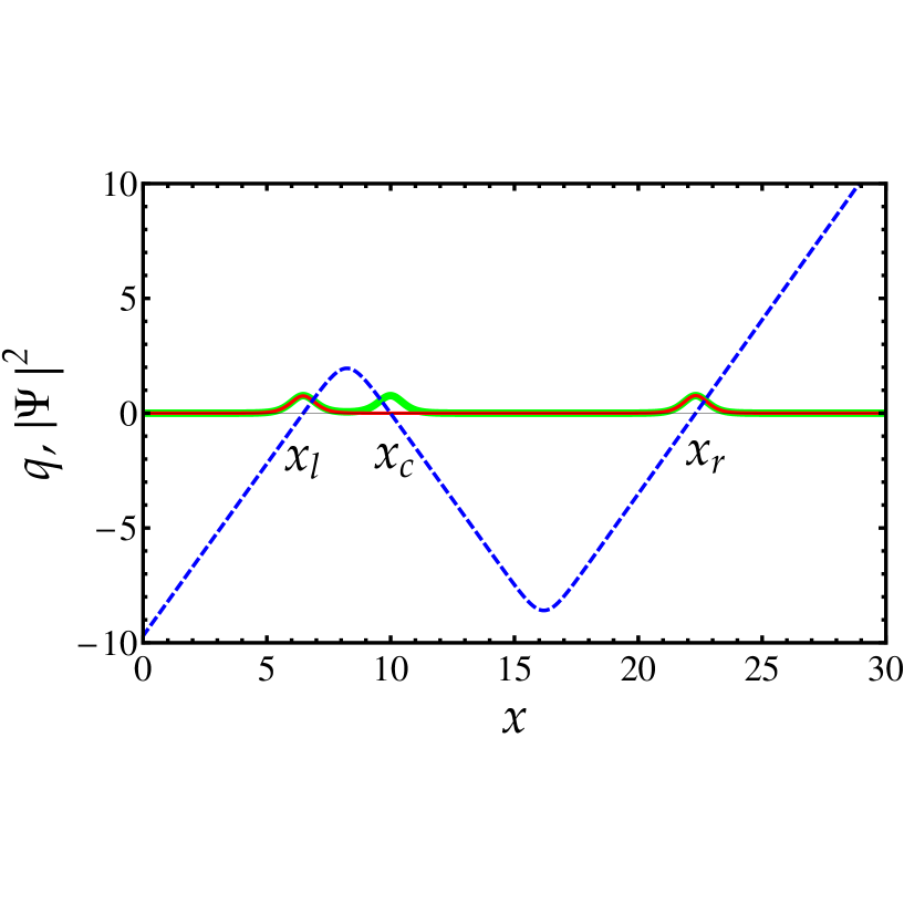
Figure 1: (Color online) Dashed (blue) curve: The argument of the second sech term in the two solitons solution, Eq. (3), $q=\alpha_{22}(t)(x-x_{\rm cm2}(t))+(1/2)\log\left[(\alpha_{1}^{2}+\alpha_{2}^{2})/(\alpha_{3}^{2}+\alpha_{4}^{2})\right]$. Thick (green) curve: The soliton intensity $|\Psi^{2}(x,t)|^{2}$. Light (red) curve: The soliton intensity with only the second sech term of Eq. (3). The parameters used are: $\gamma(t)=0$, $n_{1}=1$, $n_{2}=1.01$, $x_{1}=10$, $x_{2}=20$, $v_{1}=v_{2}=0$, $g_{0}=3$, $\phi_{01}=\phi_{02}=0$, and $t=0$.

References

• (1) A. Hasegawa and Y. Kodama, Solitons in Optical Communications (Oxford University Press, New York, 1995); L.F. Mollenauer and J.P. Gordon, Solitons in Optical Fibers (Acadamic Press, Boston, 2006); G.P. Agrawal, Nonlinear Fiber Optics (Academic Press, San Diego, 2001), 3rd ed.; N.N. Akhmediev and A. Ankiexicz, Solitons: Nonlinear Pulses and Beams (Chapman and Hall, London, 1997).
• (2) J.R. Taylor, Optical Solitons - Theory and Experiment (Cambridge University Press, Cambridge, 1992).
• (3) K.E. Strecker, G.B. Partridge, A.G. Truscott, and R.G. Hulet, Nature 417, 150 (2002).
• (4) L. Khaykovich, F. Schreck, G. Ferrari, T. Bourde, J. Cubizolles, L.D. Carr, Y. Castin, C. Salomon, Science 296, 1290 (2002).
• (5) M. Stratmann, T. Pagel, and F. Mitschke, Phys. Rev. Lett. 95, 143902 (2005).
• (6) V.I. Karpman and V.V. Solov’ev, Physica D 3, 487 (1981).
• (7) J.P. Gordon, Opt. Lett. 8, 596 (1983).
• (8) D. Anderson and M. Lisak, Opt. Lett. 11, 174 (1986).
• (9) U. Al Khawaja, H.T.C. Stoof, R.G. Hulet, K.E. Strecker, G.B. Partridge, Phys. Rev. Lett., 89, 200404 (2002).
• (10) B.A. Malomed, Phys. Rev. A 44, 6954 (1991).
• (11) V.V. Afanasjev and N. Akhmediev, Phys. Rev. E 53, 6471 (1996); V.V. Afanasjev, B.A. Malomed, and P. Chu, Phys. Rev. E 56, 6020 (1997).
• (12) N.N. Akhmediev, A. Ankiewicz, and J.M. Soto-Crespo, Phys. Rev. Lett. 79, 4047 (1997).
• (13) L. Crasovan, Y.V. Kartashov, D. Mihalache, L. Torner, Y. S. Kivshar, and V.M.P. Garcia, Phys. Rev. E 67, 046610 (2003).
• (14) A. Hause, H. Hartwig, B. Seifert, H. Stolz, M. B$\rm\ddot{o}$hm, and F. Mitschke, Phys. Rev. A 75, 063836 (2007).
• (15) A. Hause, H. Hartwig, M. B$\rm\ddot{o}$hm, and F. Mitschke, Phys. Rev. A 78, 063817 (2008).
• (16) M. Olivier and Michel Piché, Optics Express 17, 405 (2009).
• (17) A. Komarov, K. Komarov, and F. Sanchez, Phys. Rev. A 79, 033807 (2009).
• (18) A.D. Martin, C.S. Adams, and S.A. Gardiner, Phys. Rev. Lett. 98, 020402 (2007).
• (19) L. Wu, Jie-Fang Zhang, L. Li, C. Finot, and K. Porsezian, Phys. Rev. A 78, 053807 (2008).
• (20) See C. Desem and P.L. Chu in Ref.soliton_book and references theirin.
• (21) S. Raghavan and G.P. Agrawal, Opt. Commun. 180, 377 (2000).
• (22) See for instance: V.B. Matveev and M.A. Salle, Dardoux Transformations and Solitons (Springer Series in Nonlinear Dynamics, Springer-Verlag, Berlin, 1991).
• (23) U. Al Khawaja, J. Phys. A: Theor. Gen. 42, 265206 (2009).
• (24) V.N. Serkin, Akira Hasegawa, and T. L. Belyaeva, Phys. Rev. Lett. 98, 074102 (2007).
• (25) Z.X. Liang, Z.D. Zhang, and W.M. Liu, Phys. Rev. Lett. 94, 050402 (2005).
• (26) U. Al Khawaja, J. Phys. A: Theor. Gen. 39, 9679 (2006).
Refer to caption