Testing two-component jet models of GRBs with orphan afterglows

Abstract

In the Swift era, two-component jet models were introduced to explain the complex temporal profiles and the diversity of early afterglows. In this paper, we concentrate on the two-component jet model; first component is the conventional afterglow and second is the emission due to the late internal dissipation such as the late-prompt emission. We suggest herein that the two-component jet model can be probed by the existence of two optical peaks for orphan GRB afterglows. Each peak is caused by its respective jet as its relativistic beaming cone widens to encompass the off-axis line of sight. Typically, the first peak appears at $10^{4}-10^{5}$ s and the second at $10^{5}-10^{6}$ s. Furthermore, we expect to observe a single, bright X-ray peak at the same time as the first optical peak. Because orphan afterglows do not have prompt emission, it is necessary to monitor the entire sky every $10^{4}$ s in the X-ray regime. We can test the model with orphan afterglows through the X-ray all-sky survey collaboration and by using ground-based optical telescopes.

1 Introduction

The complex temporal profiles of early X-ray afterglows discovered by the Swift on-board X-ray telescope (XRT) were unexpected in the pre-Swift era. Explaining these results is one of the most difficult problems in the field of gamma-ray bursts (GRBs) (Evans et al. 2009). Most X-ray afterglows have the following three phases: steep decay, plateau, and normal decay. During the steep-decay phase, the X-ray afterglow decays with a slope of approximately $\sim-3$ or steeper: this phase extends up to $10^{2}-10^{3}$ s. The most popular interpretation of this phase attributes it to the tail of the prompt emission (Kumar & Panaitescu 2000; Zhang et al. 2006; Yamazaki et al. 2006). The plateau phase follows the steep-decay phase and begins with a slope of approximately $\sim-0.5$ or flatter and covers the time range $10^{3}-10^{4}$ s, during which a temporal break occurs. The normal decay phase then begins; the afterglow breaks and decays with a slope of approximately $\sim-1.2$, which is in agreement with the predictions of the afterglow model (Mészáros & Rees 1997; Sari et al. 1998).

However, two major problems exist with this interpretation of X-ray afterglows. The first is that the plateau phase is not completely explained by the external-shock models. To address this discrepancies, various models have been proposed, such as the energy-injection model (Nousek et al. 2006; Zhang et al. 2006; Granot & Kumar 2006), the inhomogeneous or two-component jet model (Toma et al. 2006; Eichler & Granot 2006; Granot et al. 2006), the time-dependent microphysics model (Ioka et al. 2006; Granot et al. 2006; Fan & Piran 2006), and the prior activity model (Ioka et al. 2006; Yamazaki 2009). The second problem is that the conventional afterglow models (Mészáros & Rees 1997; Sari et al. 1998) cannot explain the difference between the epoch of the breaks in light curves in the X-ray and optical observations.

Ghisellini et al. (2009) reported that the observed light curves are well explained by a two-component (early and late) jet model. Early component is responsible for the conventional afterglow emission and late component for the plateau phase. When the latter dominates the former, the X-ray light curve exhibits a plateau phase. However, there is little evidence that the early and late jet models are correct and no way to distinguish these models from other models such as the energy-injection model or the time-dependent micro-physics model. We show that observations of orphan afterglows are crucial for testing a part of the early and late jet models such as the late-prompt emission model (Ghisellini et al. 2007).

In this study, we calculate the light curves of orphan afterglows for the late-prompt emission model. We find that the two components can be distinguished in the optical regime by observing from off-axis. Therefore, if the orphan afterglows present two optical peaks, this fact becomes a strong evidence that GRB afterglows consist of two components. Moreover, we estimate the detection rate of the orphan afterglows on the basis of the late-prompt emission model and find that it would be possible to detect them and thereby test this model.

This article is organized as follows: In Section 2, we explain the motivation for considering the two-component (early and late) jet models by reviewing the results of Ghisellini et al. (2009) and introduce the late-prompt emission model. In Section 3, we describe the numerical method to calculate the off-axis light curves. The results and their qualitative interpretations are presented in Section 4. Finally, in Section 5, we summarize and discuss the possibility of observing orphan afterglows.

2 Two-component jet Model

We begin with the two-component (early and late) jet model, which explains the complex light curves, especially the plateau phase and the chromatic jet break. The model assumes that the observed GRB light curves are the sum of two components. The first component is the early emission from the forward shock due to the interaction of a fireball with the inter-stellar medium (conventional afterglow emission). The second component is caused by the late internal dissipation which produces the plateau phase. With this model, the difference in the break epoch between the X-ray and the optical regime is explained by the fact that the origin of the optical flux is different from that of the X-ray flux.

Ghisellini et al. (2009) showed that their model explains well the observed light curves; that is, the early emission and the late emission due to a central engine activity that lives long after the prompt emission. They assumed that the plateau phase is realized by the late emission, which we call the late-prompt emission which can be expressed as the broken power law

$$L\propto\left\{\begin{array}[]{ll}T^{-\alpha_{1}}&(T\leq T_{a}),\\ T^{-\alpha_{2}}&(T\geq T_{a}),\\ \end{array}\right.$$ (3)

where $T_{a}$ is the time at which the plateau phase ends, and the constants are typically $\alpha_{1}\sim 0$ and $\alpha_{2}\sim 1.6$ (Ghisellini et al. 2009).

They obtained several parameters for this model by fitting it to 33 GRBs with known redshifts. As an example, we present one of the 33 fit results in Figure 1. The lines show the fit by Ghisellini’s model; the red, blue, and black lines represent the early emission, the late-prompt emission, and their sum, respectively. The solid and dashed lines refer to the X-ray light curves and the optical light curves, respectively. The dynamics of this GRB exhibit a plateau phase in the X-ray regime but not in the optical regime. The sum of these two components describes well the light curve of the plateau phase and the normal phase in both bands. In this article, we concentrate on the late-prompt emission model and suggest a method to verify whether these two components exist.

3 Numerical Method

In this section, we describe our calculation of the off-axis light curves of the early emission and the late-prompt emission. Because of the strong beaming effect, the observed off-axis emission does not exhibit prompt emission and therein is often called the ”orphan” afterglow. Here, we define the time $T$ as the observed time elapse since the GRB trigger if the prompt emission were isotropic.

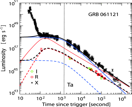
Figure 1: X-ray ($0.3-10$ keV) (black crosses) and optical (green and red circles) light curves. The lines show the fit by the two-component jet model (Ghisellini et al. 2009); the red, blue, and black lines represent the early emission, the late-prompt emission, and their sum, respectively. The solid and dashed lines refer to the X-ray light curves and the optical ones, respectively. The vertical line corresponds to $T_{a}$. The data are taken from Page et al. 2007 (and references therein).

3.1 Orphan early emission

The dynamics of the orphan early emissions have already been predicted by several authors (Totani & Panaitescu 2002; Granot et al. 2002; Granot 2005 ). Assume that a photon emitted at lab-frame time $t$ (the frame of the central engine), radius $R$, and angle $\theta$ from the line-of-sight reaches the observer at $T$. In this case, $T$ is given by $\frac{T}{1+z}=t-\frac{R\cos\theta}{c}$, where $z$ is the GRB redshift and $R$ is given by

$$R=c\int^{t}_{0}\beta(t^{\prime})dt^{\prime}\simeq ct-\int^{R}_{0}\frac{dR^{\prime}}{2\gamma^{2}},$$ (4)

for $\gamma\gg 1$. For simplicity, we assume the ”thin shell” case, for which the width and expansion of the shell are neglected in calculating its deceleration. The dynamics of the forward shock are determined by the self-similar solution (Blandford & McKee 1976). The Lorentz factor as a function of $R$ is $\gamma(R)\simeq\eta$ for $R<R_{\rm{dec}}$ and $\gamma(R)\simeq\eta(R/R_{\rm{dec}})^{-3/2}$ for $R>R_{\rm{dec}}$, where $\eta$ is the initial Lorentz factor of the shell (typically $\eta\sim 10^{2}$) and $R_{\rm{dec}}$ is the deceleration radius. With these relationships, the flux density in the thin-shell case is given by

$$F_{\nu}(T)=\frac{(1+z)}{d_{L}^{2}(z)}$$

$$\hskip 14.22636pt\times\int d^{4}x\delta\Big{(}t-\frac{T}{1+z}-\frac{R\cos\theta}{c}\Big{)}\frac{j^{\prime}_{\nu^{\prime}}}{\gamma^{2}(1-\beta\cos\theta)^{2}},$$ (5)

where $d_{L}(z)$ is the luminosity distance and $L^{\prime}_{\nu^{\prime}}$ and $\nu^{\prime}$ are the spectral luminosity in units of erg s^-1 Hz^-1 and the frequency in the comoving frame, respectively. The quantity $L^{\prime}_{\nu^{\prime}}$ may be expressed as a function of $R$ and $\nu^{\prime}$ (Sari 1998, Granot et al 2002).

By integrating the right-hand side of Eq.(3), we can express the flux density as

$$F_{\nu}(T)=\frac{(1+z)}{8\pi d_{L}^{2}(z)}\int d\cos\theta\frac{L^{\prime}_{\nu^{\prime}}(R)}{\gamma^{3}(1-\beta\cos\theta)^{3}}\frac{\Delta\phi}{2\pi},$$ (6)

where $\frac{\Delta\phi}{2\pi}$ is the correction factor when the viewing angle is larger than the jet opening angle ($\theta_{v}>\theta_{j}$). Certainly, for $\theta_{v}=0$, $\frac{\Delta\phi}{2\pi}=1$ for $0<\theta<\theta_{j}$. Outside the jet angle, the correction factor is given by

$$\frac{\Delta\phi}{2\pi}\simeq\left\{\begin{array}[]{ll}0&(\theta<\theta_{v}-\theta_{j}),\\ \frac{\phi}{\pi}&(\theta_{v}-\theta_{j}<\theta<\theta_{v}+\theta_{j}),\\ 0&(\theta_{v}+\theta_{j}<\theta),\\ \end{array}\right.$$ (10)

$$\cos\phi=\frac{\cos\theta_{j}-\cos\theta_{v}\cos\theta}{\sin\theta_{v}\sin\theta},$$ (11)

(Woods & Loeb 1999, Yamazaki et al. 2003). Using these relationships, we can integrate to obtain the flux density of the early emission received by the observer at $T$.

3.2 Orphan late-prompt emission

We apply the above formula to the off-axis late-prompt emission. We begin with a brief description of the late-prompt emission model (Ghisellini et al. 2007). This model assumes that the central engine continues after the prompt emission to create relativistic shells with smaller Lorentz factors $\gamma_{L}(T)$ and lower powers. Initially, $\gamma_{L}\gg\theta_{jL}^{-1}$, where $\theta_{jL}$ is the late-prompt jet opening angle. Then, the emission area seen from on-axis observer is the order of $(R/\gamma_{L})^{2}$ because of the beaming effect. When $\gamma_{L}$ decreases with time and becomes smaller than $\theta_{jL}^{-1}$, the emission area becomes $(R\theta_{jL})^{2}$. Thus, the observed luminosity (erg s^-1) of the late-prompt emission can be expressed as

$$L\propto\left\{\begin{array}[]{ll}R^{2}\Delta R^{\prime}j^{\prime}(T)\propto T^{-\alpha_{1}}&(T\leq T_{a}),\\ (R\theta_{j})^{2}\Delta R^{\prime}\gamma_{L}^{2}j^{\prime}(T)\propto T^{-\alpha_{2}}&(T\geq T_{a}),\\ \end{array}\right.$$ (14)

where $j^{\prime}(T)$ is the bolometric emissivity in the comoving frame and $T_{a}$ is the time when $\gamma_{L}(T_{a})=\theta_{jL}^{-1}$. When $T=T_{a}$, one sees the jet break as in the early emission. In this model, the time $T_{a}$ corresponds to the transition from the plateau phase to the normal decay phase. Moreover, assuming that $j^{\prime}(T)$ has a constant slope before and after $T_{a}$, it is shown that $\gamma_{L}(T)\propto T^{-\Delta\alpha/2}$ ($\Delta\alpha=\alpha_{2}-\alpha_{1}$). Note that the time dependence of $\gamma_{L}$ is phenomenologically introduced to explain the plateau phase. In addition, the dissipation processes responsible for the late-prompt emission would be the same as that for the prompt emission (e.g., internal shocks). Then, this model assumes that the emission occurs at a fixed radius $R$ and the observed spectrum is well approximated by the Band function (Band et al. 1993); $f(\nu)\propto\nu^{-\beta_{\rm o}}~{}(\nu^{-\beta_{\rm X}})$ for $\nu<\nu_{b}$ ($\nu>\nu_{b}$, respectively) and the indices are typically $\beta_{\rm o}\sim 0.1$ and $\beta_{\rm X}\sim 1.0$ (Ghisellini et al. 2009). With these relations, we can obtain the flux density

$$F_{\nu}(T)=\frac{(1+z)}{8\pi d_{L}^{2}(z)}\int d\cos\theta\frac{\tilde{f}(T,\nu)}{\gamma_{L}^{2}(1-\beta_{L}\cos\theta)^{2}}\frac{\Delta\phi}{2\pi},$$ (15)

where $\tilde{f}(T,\nu)\propto T^{-\alpha_{1}}f(\nu)$. By integrating the right-hand side, we can therefore obtain the off-axis light curves of the late-prompt emission just like the orphan early emission.

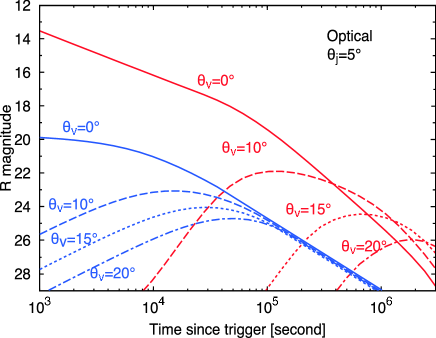
Figure 2: Optical decay curves (R-band) for the early emission (red lines) and the late-prompt emission (blue lines) when the early emission dominates the late-prompt emission. Two peaks are present, which are distinguished more clearly for larger viewing angles. The jet-opening half angle, $\theta_{j}=\theta_{Lj}=5^{\circ}$. The physical parameters of the jets are $E=10^{52}$ erg, $\epsilon_{B}=0.01$, $\epsilon_{e}=0.1$, $n=1.0$ cm^-3, $p=2.4$, $\eta=200$, $z=1$, $\alpha_{1}=0.1$, $\alpha_{2}=1.6$, $\beta_{\rm X}=0.9$, $\beta_{\rm o}=0$ and $\nu_{b}=5\times 10^{16}$ Hz, $T_{a}=10^{4}$ s, $L_{X}|_{T_{a}}=10^{47}$ erg s^-1. These parameters of the jets are taken to be typical values shown in Ghisellini et al. (2009).

4 Results

We begin with a short description for the qualitative nature of the off-axis light curves. First, we focus on the radiation from the early emission component. Because the Lorentz factor of shells producing emission initially is relativistic and the beaming effect is strong, the off-axis observer cannot see the emission. When the Lorentz factor decreases to $\theta_{v}^{-1}$, its relativistic beaming cone widens to encompass the off-axis observer. Then, the radiation can reach the off-axis observer and he observes the emission as a single peak. After that, the off-axis light curves undergo a power-law decay like the on-axis dynamics. For the early emission, the relation between the jet break time $T_{j}$ and the peak time $T_{p}$ ($\gamma\simeq\theta_{v}^{-1}$) is given by Totani & Panaitescu (2002);

$$T_{p}=\Big{(}5+2\ln\frac{\theta_{v}}{\theta_{j}}\Big{)}\Big{(}\frac{\theta_{v}}{\theta_{j}}\Big{)}^{2}T_{j}.$$ (16)

When $\theta_{v}\simeq(2-5)\times\theta_{j}$, we obtain $T_{p}\simeq 7(\theta_{v}/\theta_{j})^{2}T_{j}$.

For the late-prompt emission, the relation between the transition time $T_{a}$ and the peak time $T_{pL}$ ($\gamma_{L}\simeq\theta_{v}^{-1}$) is given by

$$T_{pL}=\Big{(}\frac{\theta_{v}}{\theta_{jL}}\Big{)}^{2/\Delta\alpha}T_{a}.$$ (17)

From Eq.(16) and Eq.(17), we have

$$\frac{T_{p}}{T_{pL}}=7\Big{(}\frac{\theta_{jL}}{\theta_{j}}\Big{)}^{2}\frac{T_{j}}{T_{a}},$$ (18)

where we set $\Delta\alpha=1$. Unfortunately, the magnitude relation of the two jet opening angles ($\theta_{jL}$ and $\theta_{j}$) is an uncertainty. When the jet opening angle of the late-prompt emission is larger than that of the early emission $\theta_{jL}\geq\theta_{j}$, we obtain $(T_{p}/T_{pL})>$ a few $(T_{j}/T_{a})$. Thus, we find $T_{p}\simeq(10-100)\times T_{pL}$ because typically $T_{j}\simeq 10^{5}-10^{6}$ s and $T_{a}\simeq 10^{4}$ s from the observational facts. If the peak amplitudes of the early emission and the late-prompt emission are the same order, therefore, we are able to observe two peaks in the light curve by viewing from off-axis. On the other hand, when the late-prompt emission is encompassed by the early emission, i.e., $\theta_{jL}<\theta_{j}$, the peak times of each emission can become the same order ($T_{p}\sim T_{pL}$) . In this case, even if the peak fluxes of two emissions are the same order, the two peaks overlap and are difficult to distinguish clearly. In this paper, we concentrate on the case of $\theta_{jL}\simeq\theta_{j}$.

Next, we present the results of our calculation and explain the behavior of the early emission and the late-prompt emission. Figure 2 and 3 show the optical and X-ray light curves, respectively, for various viewing angles ($\theta_{v}=0^{\circ}$, $10^{\circ}$, $15^{\circ}$, and $20^{\circ}$) relative to the center of the jet ($\theta_{j}=\theta_{jL}=5^{\circ}$). In Figure 4, we present the observed optical light curves: that is, the sum of the early emission and the late-prompt emission.

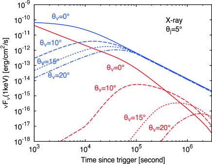
Figure 3: X-ray light curves (1 keV) for the early emission (red lines) and the late-prompt emission (blue lines) when the late-prompt emission dominates the early emission. The light curves observed off-axis (the early emission plus the late-prompt emission) have a single peak. The physical parameters used for the jets are the same as for Figure 2.

In Figure 2, we show the optical light curves for various viewing angle when the early emission (red lines) dominates the late-prompt emission (blue lines). In this case, as shown in Figure 2, we can observe the optical flux with two peaks due to the orphan early emission and the orphan late-prompt emission viewing from off-axis because both peak amplitudes are the same order. In addition, we find that the two peaks are more clearly distinguished and each peak becomes dimmer for larger viewing angle (see Figure 4). By observing two peaks in the optical, therefore, we can verify that GRB light curves consist of two components or not.

In Figure 3, we show the light curves when the X-ray flux is dominated by the late-prompt emission. According to Ghisellini et al. (2009), the X-ray flux is dominated by the late-prompt emission or by a mixture of both emissions. In this case, the observed off-axis light curves (the sum of red and blue lines for each viewing angle $\theta_{v}$) have a single peak because the early emission is dominated by the late-prompt emission. As show in Figure 3, the amplitude ratio (on/off) for the early emission is larger than the amplitude ratio for the late-prompt emission and the early emission’s peak decreases at a great rate than the late-prompt emission’s peak as the viewing angle increases. Thus, for larger viewing angle, the late-prompt emission always dominates the early emission and the characteristic that the observed light curves have a single peak does not change.

Furthermore, since the transition at $T_{a}$ corresponds to a phenomenon like the jet break in this model, the peak amplitude observed off-axis is three to five orders of magnitude larger than that expected from the conventional models (due to the orphan early emission). Thus, we can observe more orphan afterglows than expected from the conventional models if the plateau phase is attributed to the late-prompt emission. For these reasons, X-ray observation facilitates the detection of orphan GRB afterglows.

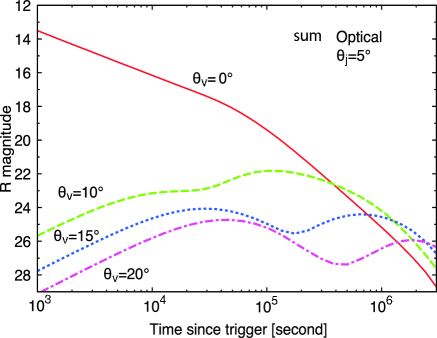
Figure 4: Observed optical light curves (R-band); sum of the early emission and the late-prompt emission. The physical parameters are the same as in Figure 2.

5 Summary & Discussion

In this study, we consider the late-prompt emission model and calculate the off-axis observed light curves. Then, we find that the off-axis observer is able to see the emission with two peaks in the optical (Figure 4) and with a single peak in the X-ray (Figure 3). We here suggest a method to test whether two components actually exist or not by applying the characteristics of off-axis light curves.

In this section, we discuss the possibility of observing the emission from off-axis. As seen in Section 4, in the late-prompt model, the single peak in the X-ray regime is roughly as bright as the flux amplitude at the transition time $T_{a}$. Then, we expect that the emission with a single peak in the X-ray is observable. We can easily estimate the detection rate of the X-ray flux viewed off-axis for the late-prompt model by using the same samples as in Ghisellini et al. (2009). Assuming that the properties of GRBs are not affected by the accuracy with which the redshift is determined, we can extrapolate the flux distribution of all Swift bursts from the above samples. Here, we suppose that the average jet angle of the GRBs is 5^∘. Next, the real number $N_{\rm{real}}(F)$ of GRBs per year for flux $F$ is not the number $N_{\rm{obs}}(F)$ of GRBs inferred from observations, but $2N_{\rm{obs}}(F)/(1-\cos\theta_{j})$. From our calculation, we find the relationship between the viewing angle $\theta_{v}$ and the peak flux for the late-prompt emission to be $F_{\rm{peak}}(\theta_{v})\propto\theta_{v}^{-2.09}$ ($\theta_{v}>\theta_{j}$). The detection rate $N_{\rm{exp}}$ is then estimated as

$$N_{\rm{exp}}=\int\frac{d\phi d\cos\theta_{v}}{4\pi}N_{\rm{real}}(F_{\rm{peak}}(\theta_{v})>F_{\rm{lim}}),$$ (19)

where $F_{\rm{lim}}$ is the instrument sensitivity.

Because the GRB observed off-axis do not have the prompt emission, the all-sky survey that monitors the whole sky is necessary to detect the single peak in the X-ray. For example, such peak with duration time of $10^{4}$ s can be detected by the current X-ray survey missions with Monitor of All-sky X-ray Image (MAXI) (Matsuoka et al. 2009). The sensitivity of MAXI is 20 mCrab ($7\times 10^{-10}$ erg cm^-2 s^-1 over the energy band $2-30$ keV) for observations during a single orbit. Because MAXI observes a point of sky every $90$ min, it is suitable for detecting the peak. In this case, the detection rate by MAXI is estimated to be $\sim 0.41$ events per year. As seen Figure 3, the peak amplitudes of the orphan late-prompt emission are a little lower than the MAXI sensitivity. In case of the orphan late-prompt emission, however, the number of GRBs whose relativistic beaming cones encompass the observer increases by a factor of $(1-\cos\theta_{v})/(1-\cos\theta_{j})$. The event rate we estimate is as much as the event rate that MAXI detects on-axis afterglows without prompt emissions. This forecast is an important outcome of the late-prompt model. Because the angular resolution of MAXI is about 0.1 arcminute, we can follow up the afterglows with ground-based optical telescopes (e.g., Gamma-Ray Burst Optical/Near-Infrared Detector; GROND) and observe emission with two peaks. Typical amplitudes of the first peak are about $24$ to $25$ in R-band magnitude. Because this sensitivity is of the same order as that of GROND (Greiner et al. 2008), it should be possible to observe the first optical peak. Although the second peak is slightly dimmer than the first, we consider that after a few days, the second peak can be observed by GROND or the larger optical telescopes. Seven bands of GROND observation help to distinguish the afterglows from other variables. The second peak, which has a synchrotron spectrum because of the external shock, can be distinguished from supernovae.

In this study, we calculate the off-axis light curves in the late-prompt model by integrating the analytical expressions. However, in recent study, van Eerten, Zhang & MacFadyen (2010) show that the off-axis light curves calculated analytically are different from the results with a two-dimensional axisymmetric hydrodynamics simulation. Then, it is significant to calculate the off-axis late-prompt emission in order to discuss whether two peaks are distinguishable. Furthermore, the late-prompt emission model assumes the radius $R$ to be constant. If the radius expands of the emission area, the peak time $T_{pL}$ for the late-prompt emission more delays in the same way as the peak time $T_{p}$ for the early emission as the viewing angle increases. In this case, it may be, therefore, difficult to distinguish the optical two peaks in the optical with the observation of orphan afterglows.

Finally, we mention other late-internal dissipation models. In these models, the transition time $T_{a}$ does not necessarily correspond to the jet break but to the time scale for the matter accretion (Kumar et al. 2008) or the spin-down time scale for the magnetar scenarios (Zhang & Mészáros 2001; Thompson et al. 2004). If this is the case, then the Lorentz factor evolution history of the late outflow is unpredictable, and the predicted orphan afterglow light curves would be subject to even larger uncertainties. In future works, we should discuss other possibilities for testing two-component jet models. Nevertheless, if we observe a characteristic light curve, which has a bright single peak in the X-ray and two peaks in the optical, we obtain an evidence that GRBs light curves are composed of the early and late jet, and may restrict other models than the early and late jet model.

We would like to thank T. Nakamura for his continuous encouragement and K. Murase, K. Yagi, M. Hayashida, S. Inoue, Y. Inoue, and Y. Doleman for useful discussions. This work is supported in part by the Grant-in-Aid for the global COE program The Next Generation of Physics, Spun from Universality and Emergence at Kyoto University. RT is supported by a Grant-in-Aid for the Japan Society for the Promotion of Science (JSPS) Fellows and is a research fellow of JSPS.

References

- [Band et al.(1993)] Band, D., et al. 1993, ApJ, 413, 281
- [Blandford & McKee(1976)] Blandford, R. D., & McKee, C. F. 1976, Physics of Fluids, 19, 1130
- [Eichler & Granot(2006)] Eichler, D., & Granot, J. 2006, ApJ, 641, L5
- [Evans et al.(2009)] Evans, P. A., et al. 2009, MNRAS, 397, 1177
- [Fan & Piran(2006)] Fan, Y., & Piran, T. 2006, MNRAS, 369, 197
- [Ghisellini et al.(2007)] Ghisellini, G., Ghirlanda, G., Nava, L., & Firmani, C. 2007, ApJ, 658, L75
- [Ghisellini et al.(2009)] Ghisellini, G., Nardini, M., Ghirlanda, G., & Celotti, A. 2009, MNRAS, 393, 253
- [Granot(2005)] Granot, J. 2005, ApJ, 631, 1022
- [Granot et al.(2006)] Granot, J., Königl, A., & Piran, T. 2006, MNRAS, 370, 1946
- [Granot & Kumar(2006)] Granot, J., & Kumar, P. 2006, MNRAS, 366, L13
- [Granot et al.(2002)] Granot, J., Panaitescu, A., Kumar, P., & Woosley, S. E. 2002, ApJ, 570, L61
- [Greiner et al.(2008)] Greiner, J., et al. 2008, PASP, 120, 405
- [Ioka et al.(2006)] Ioka, K., Toma, K., Yamazaki, R., & Nakamura, T. 2006, A&A, 458, 7
- [Kumar et al.(2008)] Kumar, P., Narayan, R., & Johnson, J. L. 2008, MNRAS, 388, 1729
- [Kumar & Panaitescu(2000)] Kumar, P., & Panaitescu, A. 2000, ApJ, 541, L51
- [Matsuoka et al.(2009)] Matsuoka, M., et al. 2009, PASJ, 61, 999
- [Meszaros & Rees(1997)] Mészáros, P. & Rees, M. J. 1997, ApJ, 476, 232
- [Nousek et al.(2006)] Nousek, J. A., et al. 2006, ApJ, 642, 389
- [Page et al.(2007)] Page, K. L., et al. 2007, ApJ, 663, 1125
- [Sari(1998)] Sari, R. 1998, ApJ, 494, L49
- [Sari et al.(1998)] Sari, R., Piran, T., & Narayan, R. 1998, ApJ, 497, L17
- [Thompson et al.(2004)] Thompson, T. A., Chang, P., & Quataert, E. 2004, ApJ, 611, 380
- [Toma et al.(2006)] Toma, K., Ioka, K., Yamazaki, R., & Nakamura, T. 2006, ApJ, 640, L139
- [Totani & Panaitescu(2002)] Totani, T., & Panaitescu, A. 2002, ApJ, 576, 120
- [van Eerten et al.(2010)] van Eerten, H., Zhang, W., & MacFadyen, A. 2010, ApJ, 722, 235
- [Woods & Loeb(1999)] Woods, E., & Loeb, A. 1999, ApJ, 523, 187
- [Yamazaki(2009)] Yamazaki, R. 2009, ApJ, 690, L118
- [Yamazaki et al.(2003)] Yamazaki, R., Ioka, K., & Nakamura, T. 2003, ApJ, 593, 941
- [Yamazaki et al.(2006)] Yamazaki, R., Toma, K., Ioka, K., & Nakamura, T. 2006, MNRAS, 369, 311
- [Zhang et al.(2006)] Zhang, B., Fan, Y. Z., Dyks, J., Kobayashi, S., Mészáros, P., Burrows, D. N., Nousek, J. A., & Gehrels, N. 2006, ApJ, 642, 354
- [Zhang & Mészáros(2001)] Zhang, B., & Mészáros, P. 2001, ApJ, 552, L35