Fluctuations of the Josephson current and electron-electron interactions in superconducting weak links

Abstract

We derive a microscopic effective action for superconducting contacts with arbitrary transmission distribution of conducting channels. Provided fluctuations of the Josephson phase remain sufficiently small our formalism allows to fully describe fluctuation and interaction effects in such systems. As compared to the well studied tunneling limit our analysis yields a number of qualitatively new features which occur due to the presence of subgap Andreev bound states in the system. We investigate the equilibrium supercurrent noise and evaluate the electron-electron interaction correction to the Josephson current across superconducting contacts. At $T=0$ this correction is found to vanish for fully transparent contacts indicating the absence of Coulomb effects in this limit.

I Introduction

It is well known that supercurrent can flow through a non-superconducting barrier between two superconducting reservoirs. Initially this effect was predicted BJ and microscopically analyzed AB for a specific case of (usually very thin) tunnel insulating barriers. Later it was understood that non-dissipative transport of Cooper pairs between two superconductors is also possible in many other types of weak links, such as, e.g., quantum point contacts KO and superconductor-normal-metal-superconductor ($SNS$) junctions SNScl ; SNSd , i.e. if a piece of a normal metal is placed in-between two superconductors. In contrast to tunnel junctions, in $SNS$ systems at sufficiently low temperatures appreciable supercurrent can flow even though a normal layer can be as thick as few microns.

It turned out that the Josephson effect in superconducting weak links without tunnel barriers is directly related to another fundamentally important phenomenon: Andreev reflection AR . Suffering Andreev reflections at both $NS$ interfaces, quasiparticles with energies below the superconducting gap are effectively “trapped” inside the junction forming a discrete set of levels which can be tuned by passing the supercurrent across the system. At the same time, these subgap Andreev levels themselves contribute to the supercurrent thus making the behavior of superconducting point contacts and $SNS$ junctions in many respects different from that of tunnel barriers. For an extended review summarizing various features of dc Josephson effect in different types of superconducting weak links we refer the reader to Refs. lam, ; bel, ; SaMiZhe, .

The number of Cooper pairs transferred between two superconductors and, hence, the Josephson current can fluctuate around its mean value Madrid ; Averin ; Yip . While at non-zero temperatures thermal fluctuations of the supercurrent should naturally exist in all types of weak links, in the limit $T\to 0$ the relevant physics is essentially determined by the presence or absence of subgap Andreev states. Provided such states are present fluctuations of the supercurrent do in general occur even at $T=0$ and at subgap frequencies. E.g., the equilibrium supercurrent correlation functions show pronounced peaks at frequencies equal to the distance between Andreev levels inside the weak link. The amplitudes of such peaks turn out to scale as Madrid $\sum_{n}T_{n}^{2}(1-T_{n})$, where $T_{n}$ is the normal transmission of the $n$-th conducting mode of the barrier and the sum is taken over all such modes. The latter dependence implies that ground state fluctuations of the supercurrent can be expected neither in the limit of low barrier transmissions $T_{n}\to 0$ (i.e. in tunnel barriers where no Andreev states are present) nor in fully open contacts with $T_{n}\to 1$.

Note that the above considerations remain applicable if one can neglect Coulomb effects. In small-size superconducting contacts, however, such effects can be important and should in general be taken into account. A lot is known about interplay between fluctuations and charging effects in superconducting tunnel barriers SZ . Here we examine the properties of superconducting junctions going beyond the tunneling limit. We will analyze fluctuation and interaction effects and demonstrate that Coulomb blockade in such junctions weakens with increasing barrier transmissions and eventually disappears in the limit of fully open superconducting contacts.

The structure of our paper is as follows. In Sec. II we derive an effective action for superconducting contacts with arbitrary distribution of channel transmissions which enables one to describe equilibrium fluctuations of the current and interaction effects. In Sec. III we make use of this action and evaluate the supercurrent noise in superconducting contacts. Low frequency current response and capacitance renormalization due to retardation effects are discussed in Sec. IV. In Sec. V we analyze the interaction correction to the Josephson current. A brief summary of our main results is presented in Sec. VI. Some general expressions and technical details are relegated to Appendix.

II Effective action and phase fluctuations

In what follows we will adopt the standard model of a superconducting contact and consider two big superconductors connected with each other via a normal conductor (see Fig. 1) characterized by arbitrary transmission distribution $T_{n}$ of its spin-degenerate conducting channels. Below we will only consider the limit of sufficiently short normal conductors with effective Thouless energy $\varepsilon_{\rm Th}$ strongly exceeding the superconducting gap $\Delta$ in both reservoirs, $\varepsilon_{\rm Th}\gg\Delta$. In addition, the normal conductor length is assumed to be much shorter than dephasing and inelastic relaxation lengths. Coulomb interaction between electrons in the contact area is described in a standard manner by an effective capacitance $C$.

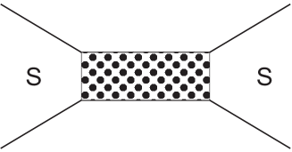
Figure 1: Short coherent conductor between two superconducting reservoirs.

We will assume that the contact is biased by external current $I$ which does not exceed the critical one $I_{C}$ and, hence, can flow through the contact without any dissipation, i.e. $I\equiv I_{S}$. In the absence of fluctuations this external current sets the value of the order parameter phase difference $\chi=\chi_{L}-\chi_{R}$ between two superconductors. The corresponding implicit dependence of $\chi$ on the supercurrent $I_{S}$ has the form KO

$$I_{S}(\chi)=\frac{e\Delta\sin\chi}{2}\sum_{n}\frac{T_{n}}{\sqrt{1-T_{n}\sin^{2}(\chi/2)}}$$ (1)

$$\times\tanh\frac{\Delta\sqrt{1-T_{n}\sin^{2}(\chi/2)}}{2T}.$$

Here and below we set $\hbar=1$ and define the electron charge to be $-e$.

In order to analyze fluctuation and interaction effects in such superconducting contacts we will allow for fluctuations of the superconducting phase difference around its average value $\chi$ and employ the effective action formalism combined with the scattering matrix technique. This approach was proven to be very successful in the case of normal conductors GZ01 ; GGZ03 ; KN ; GZ04 and NS hybrid structures GZ06 ; GZ09 . Following the usual procedure we express the kernel $J$ of the evolution operator on the Keldysh contour in terms of a path integral over the fermionic fields which can be integrated out after the standard Hubbard-Stratonovich decoupling of the interacting term SZ . Then the kernel $J$ acquires the form

$$J=\int{\cal D}\varphi_{1}{\cal D}\varphi_{2}\exp(iS_{c}[\varphi]+iS_{t}[\varphi]),$$ (2)

where the terms $S_{c}[\varphi]$ and $S_{t}[\varphi]$ account respectively for charging effects and for the transfer of electrons and Cooper pairs between two superconducting reservoirs. Both these terms represent the functionals of the fluctuating phase variables $\varphi_{1,2}(t)$ defined on the forward and backward parts of the Keldysh contour and related to fluctuating voltages $V_{1,2}$ across the conductor as $\dot{\varphi}_{1,2}(t)=eV_{1,2}$. With the aid of the Josephson relation one trivially identifies the superconducting phase difference on two branches of the Keldysh contour as $\chi+2\varphi_{1,2}(t)$.

The charging term is taken in the standard form SZ

$$S_{c}[\varphi]=\frac{C}{2e^{2}}\int\limits_{0}^{t}dt^{\prime}(\dot{\varphi}_{1}^{2}-\dot{\varphi}_{2}^{2})\equiv\frac{C}{e^{2}}\int\limits_{0}^{t}dt\dot{\varphi}^{+}\dot{\varphi}^{-},$$ (3)

where we also introduced “classical” and “quantum” parts of the phase, respectively $\varphi_{+}=(\varphi_{1}+\varphi_{2})/2$ and $\varphi_{-}=\varphi_{1}-\varphi_{2}$. The structure of the term $S_{t}[\varphi]$ is the same as in the normal case, one should only replace normal propagators by $2\times 2$ Green-Gorkov matrix functions SZ ; Z ; SN . The corresponding result can be expressed in the form SN

$$S_{t}[\varphi]=-\frac{i}{2}\sum_{n}{\rm Tr}\ln\left[1+\frac{T_{n}}{4}\left(\left\{\check{Q}_{L}(\varphi),\check{Q}_{R}\right\}-2\right)\right],$$ (4)

where $\check{Q}_{L,R}$ are $4\times 4$ Green-Keldysh matrices of the left and right superconducting electrodes. The product of these matrices implies time convolution and curly brackets denote anticommutation.

Without loss of generality we can set the electric potential (and, hence, fluctuating phases) of the right superconducting terminal equal to zero. Then the Green-Keldysh matrix of this electrode can be written in a simple form

$$\check{Q}_{R}=\check{g}=\left(\begin{array}[]{cc}\hat{g}^{R}&\hat{g}^{K}\\ 0&\hat{g}^{A}\end{array}\right),$$ (5)

where $\hat{g}^{R,A}$ are retarded and advanced $2\times 2$ matrix functions

$$\hat{g}^{R,A}=\frac{\epsilon\hat{\tau}_{3}+\hat{\Delta}}{\xi^{R,A}},\quad\xi^{R,A}=\pm\sqrt{(\epsilon\pm i\delta)^{2}-\Delta^{2}}$$ (6)

and $\hat{g}^{K}=\hat{g}^{R}F-F\hat{g}^{A}$ is the Keldysh matrix, where $F(\epsilon)=\tanh(\epsilon/2T)$ is the Fourier transform of $F(t)=-iT/\sinh[\pi Tt]$ and $\hat{\tau}_{i}$ are the Pauli matrices. For simplicity we choose the order parameter $\Delta$ of the right superconductor real and, hence, we can set $\hat{\Delta}=i\Delta\hat{\tau}_{2}$. In order to properly account for analytic properties of the functions $\xi^{R,A}$ here we keep an infinitesimally small imaginary part $i\delta$ which allows to define $\xi^{R,A}=\pm{\rm sgn}\,\epsilon\sqrt{\epsilon^{2}-\Delta^{2}}$ for $|\epsilon|>\Delta$ and $\xi^{R,A}=i\sqrt{\Delta^{2}-\epsilon^{2}}$ for $|\epsilon|<\Delta$.

The Green-Keldysh matrix $\check{Q}_{L}$ of the left superconducting electrode reads

$$\check{Q}_{L}(\varphi)(t,t^{\prime})=\check{\cal L}\check{\cal M}_{+}(t)\check{\cal L}\check{g}(t,t^{\prime})\check{\cal L}\check{\cal M}_{-}(t^{\prime})\check{\cal L},$$ (7)

where we defined the matrices

$$\check{\cal L}=\frac{1}{\sqrt{2}}\left(\begin{array}[]{cc}\hat{1}&\hat{1}\\ \hat{1}&-\hat{1}\end{array}\right)$$

and

$$\check{\cal M}_{\pm}=$$

$$\left(\begin{array}[]{cc}\exp\left[\pm i\left(\frac{\chi}{2}+\varphi_{1}(t)\right)\hat{\tau}_{3}\right]&0\\ 0&\exp\left[\pm i\left(\frac{\chi}{2}+\varphi_{2}(t)\right)\hat{\tau}_{3}\right]\end{array}\right).$$ (10)

Substituting the above expressions for $\check{Q}_{L}$ and $\check{Q}_{R}$ into Eq. (4) we arrive at the action which fully describes transfer of electrons and Cooper pairs to all orders in $T_{n}$. In the case of tunnel barriers the channel transmissions remain small and one can expand $S_{t}$ in powers of $T_{n}$. Keeping the lowest order terms $\sim T_{n}$ of this expansion one recovers the well-known Ambegaokar-Eckern-Schön (AES) action SZ . Here, however, we will go beyond the tunneling limit and analyze fluctuation effects at arbitrary transmission values $T_{n}$.

To this end we will proceed similarly to Ref. GZ09, and introduce the matrix

$$\check{X}_{0}=1-T_{n}/2+(T_{n}/4)\left\{\check{Q}_{L},\check{Q}_{R}\right\}|_{\varphi_{\pm}=0}.$$ (11)

As the action $S_{t}$ vanishes for $\varphi_{-}(t)=0$ one has ${\rm Tr}\ln\check{X}_{0}=0$. Making use of this property we can identically transform the action (4) to

$$S_{t}=-\frac{i}{2}\sum_{n}{\rm Tr}\ln\left[1+\check{X}_{0}^{-1}\circ\check{X}^{\prime}\right],$$ (12)

where

$$\check{X}^{\prime}=1+(T_{n}/4)\left(\left\{\check{Q}_{L},\check{Q}_{R}\right\}-2\right)-\check{X}_{0}.$$ (13)

With the aid of the above expressions for $\check{Q}_{L,R}$ we obtain

$$\check{X}_{0}^{-1}=\left(\begin{array}[]{cc}\frac{\xi^{2}\hat{1}}{(\epsilon+i\delta)^{2}-\epsilon_{n}^{2}}&\frac{-i\pi\xi^{2}\hat{1}}{\epsilon_{n}}\tanh\frac{\epsilon_{n}}{2T}\sum_{\pm}\delta(\epsilon\pm\epsilon_{n})\\ 0&\frac{\xi^{2}\hat{1}}{(\epsilon-i\delta)^{2}-\epsilon_{n}^{2}}\end{array}\right),$$ (14)

where $\xi^{2}=\epsilon^{2}-\Delta^{2}$ and the subgap Andreev level inside the contact with energies $\pm\epsilon_{n}(\chi)$ are defined in a usual way as

$$\epsilon_{n}(\chi)=\Delta\sqrt{1-T_{n}\sin^{2}(\chi/2)}.$$ (15)

Now let us assume that fluctuating phases $\varphi_{\pm}(t)$ (or fluctuating voltages) at the junction are sufficiently small and perform regular expansion of the exact effective action in powers of these phases. Expanding $\check{Q}_{L}(\varphi)$ up to the second order in $\varphi_{\pm}$ (thus finding the matrix $\check{X}^{\prime}$), from Eq. (12) we obtain

$$iS_{t}=-\frac{i}{e}\int\limits_{0}^{t}dt^{\prime}I_{S}(\chi)\varphi_{-}(t^{\prime})+iS_{R}-S_{I},$$ (16)

where the supercurrent $I_{S}(\chi)$ is defined in Eq. (1) and

$$S_{R} = \int\limits_{0}^{t}dt^{\prime}\int\limits_{0}^{t}dt^{\prime\prime}{\cal R}(t^{\prime}-t^{\prime\prime})\varphi^{-}(t^{\prime})\varphi^{+}(t^{\prime\prime}),$$ (17)

$$S_{I} = \int\limits_{0}^{t}dt^{\prime}\int\limits_{0}^{t}dt^{\prime\prime}{\cal I}(t^{\prime}-t^{\prime\prime})\varphi^{-}(t^{\prime})\varphi^{-}(t^{\prime\prime})$$ (18)

with both kernels ${\cal R}(t)$ and ${\cal I}(t)$ being real functions. The general expressions for these functions turn out to be somewhat lengthy and for this reason are presented in Appendix. Here we only emphasize some of the properties of ${\cal R}(t)$ and ${\cal I}(t)$.

To begin with, it is straightforward to verify that in the lowest order in barrier transmissions $T_{n}$ the result (16)-(18) reduces to the standard AES action SZ for tunnel barriers in the limit of small phase fluctuations. Qualitatively new features emerge in higher orders in $T_{n}$ being directly related to the presence of subgap Andreev levels $\pm\epsilon_{n}(\chi)$ inside the contact. Consider, for instance, the kernel ${\cal I}(t)$ defined in Eq. (62). It can be split into three contributions of different physical origin

$${\cal I}(t)={\cal I}_{1}(t)+{\cal I}_{2}(t)+{\cal I}_{3}(t).$$ (19)

The first of these terms, ${\cal I}_{1}(t)$, represents the subgap contribution due to discrete Andreev states. The Fourier transform of this term has the form (cf. the first line in Eq. (62))

$${\cal I}_{1\omega}=\frac{\pi\Delta^{4}}{4}\sum_{n}\bigg{\{}\frac{T_{n}^{2}\sin^{2}\chi}{2\epsilon_{n}^{2}(\chi)\cosh^{2}(\epsilon_{n}(\chi)/2T)}\delta(\omega)$$

$$+\frac{T_{n}^{2}(1-T_{n})\sin^{4}(\chi/2)}{\epsilon^{2}_{n}(\chi)}\left[1+\tanh^{2}(\epsilon_{n}(\chi)/2T)\right]$$

$$\times[\delta\left(\omega-2\epsilon_{n}(\chi)\right)+\delta\left(\omega+2\epsilon_{n}(\chi)\right)]\bigg{\}}.$$ (20)

It is obvious that this contribution is not contained in the AES action at all. The general expression for the second term ${\cal I}_{2}(t)$ is defined by the second and third lines of Eq. (62). In the limit of small barrier transmissions this term scales as ${\cal I}_{2}\propto T_{n}^{3/2}$ and, hence, is not contained in the AES action either. This contribution can be interpreted as the ”interference term” between subgap Andreev levels and quasiparticle states above the gap. In the low temperature limit $T\to 0$ the Fourier transform of this term ${\cal I}_{2\omega}$ differs from zero only at sufficiently high frequencies $|\omega|>\Delta+\epsilon_{n}(\chi)$. At higher temperatures $T\gtrsim\epsilon_{n}(\chi)$, however, ${\cal I}_{2\omega}$ vanishes only for $|\omega|<\Delta-\epsilon_{n}(\chi)$ and remains non-zero otherwise. Finally, the third term ${\cal I}_{3}(t)$ accounts for the contribution of quasiparticles with energies above the gap. The Fourier transform of this term ${\cal I}_{3\omega}$ is defined by the fourth and fifth lines of Eq. (62). In the high frequency limit $\omega\gg\Delta$ or for $\Delta\to 0$ this term reduces to the standard result for a normal conductor

$${\cal I}_{3\omega}\to\frac{\omega}{2e^{2}R_{N}}\coth\frac{\omega}{2T},$$ (21)

where $R_{N}$ is the normal contact resistance determined by the Landauer formula

$$\frac{1}{R_{N}}=\frac{e^{2}}{\pi}\sum_{n}T_{n}.$$ (22)

Turning now to the function ${\cal R}(t)$ in Eq. (17) we note that its Fourier transform can be represented as ${\cal R}_{\omega}={\cal R}^{\prime}_{\omega}+i{\cal R}^{\prime\prime}_{\omega}$, where both ${\cal R}^{\prime}_{\omega}$ and ${\cal R}^{\prime\prime}_{\omega}$ are real functions. The function ${\cal R}^{\prime}_{\omega}$ is even in $\omega$ while ${\cal R}^{\prime\prime}_{\omega}$ is an odd function of $\omega$, thus implying that the function ${\cal R}(t)$ is real.

The functions ${\cal R}(t)$ and ${\cal I}(t)$ are not independent. For instance, the Fourier transform ${\cal R}^{\prime\prime}_{\omega}$ is related to ${\cal I}_{\omega}$ by means of the fluctuation-dissipation relation

$${\cal R}^{\prime\prime}_{\omega}=2{\cal I}_{\omega}\tanh\frac{\omega}{2T}.$$ (23)

The two functions ${\cal R}^{\prime}_{\omega}$ and ${\cal R}^{\prime\prime}_{\omega}$ are in turn linked to each other by the causality principle: the function ${\cal R}(t)$ should vanish for $t<0$. The general expression for ${\cal R}^{\prime}_{\omega}$ (63) and further details are presented in Appendix.

Finally we would like to point out that with the aid of the above Gaussian effective action one can easily evaluate the phase-phase correlation functions for our problem. Combining Eqs. (16)-(18) with (3) one finds

$$\langle\varphi_{+}(t_{1})\varphi_{+}(t_{2})\rangle=$$ (24)

$$-\int\limits_{-\infty}^{\infty}\frac{d\omega}{2\pi}{\rm Im}\left(\frac{1}{C\omega^{2}/e^{2}+{\cal R}_{\omega}}\right)\coth\frac{\omega}{2T}e^{-i\omega(t_{1}-t_{2})},$$

$$\langle\varphi_{+}(t_{1})\varphi_{-}(t_{2})\rangle=$$

$$i\int\limits_{-\infty}^{\infty}\frac{d\omega}{2\pi}\left(\frac{1}{{C\omega^{2}/e^{2}+\cal R}_{\omega}}\right)e^{-i\omega(t_{1}-t_{2})},$$

$$\langle\varphi_{-}(t_{1})\varphi_{-}(t_{2})\rangle=0.$$

Note that these expressions do not include the effect of (possibly existing) external impedance which we do not specify here. If needed, corresponding modifications can easily be implemented in a standard manner SZ .

In addition to the above phase-phase correlation functions in what follows we will also need to define the expectation value of the current operator

$$\langle\hat{I}(t)\rangle=ie\int{\cal D}\varphi_{\pm}\frac{\delta}{\delta\varphi_{-}(t)}e^{iS_{c}[\varphi]+iS_{t}[\varphi]}$$ (25)

and the current-current correlation function $\langle\hat{I}(t)\hat{I}(t^{\prime})\rangle$. For the symmetrized version of this correlator we have

$$\langle\hat{I}(t)\hat{I}(t^{\prime})+\hat{I}(t^{\prime})\hat{I}(t)\rangle$$

$$=-2e^{2}\int{\cal D}\varphi_{\pm}\frac{\delta^{2}}{\delta\varphi_{-}(t)\delta\varphi_{-}(t^{\prime})}e^{iS_{c}[\varphi]+iS_{t}[\varphi]}.$$ (26)

III Equilibrium supercurrent noise

We first employ our results in order to describe fluctuation effects in superconducting contacts in the absence of electron-electron interactions. In this case after performing functional derivatives with respect to $\varphi_{-}(t)$ in Eqs. (25) and (26) one should formally set $\varphi_{-}=0$.

Let us define the noise spectrum ${\cal S}_{\omega}$ as

$$\frac{1}{2}\langle\hat{I}(t_{1})\hat{I}(t_{2})+\hat{I}(t_{2})\hat{I}(t_{1})\rangle-I_{S}^{2}=\int\limits_{-\infty}^{\infty}\frac{d\omega}{2\pi}{\cal S}_{\omega}e^{-i\omega(t_{1}-t_{2})}.$$ (27)

Then from Eq. (26) for $\omega\ll 1/R_{N}C$ we easily find

$${\cal S}_{\omega}=2e^{2}{\cal I}_{\omega}.$$ (28)

Together with Eq. (62) this result provides the complete expression for the equilibrium noise power spectrum in superconducting contacts with arbitrary distribution of channel transmissions $T_{n}$.

In the low temperature limit $T\to 0$ and at subgap frequencies $0\leq\omega<2\Delta$ the above general result reduces to the following expression

$${\cal S}_{\omega}=e^{2}\sum_{n}\bigg{\{}\frac{\pi\Delta^{2}T_{n}^{2}(1-T_{n})\sin^{4}(\chi/2)}{1-T_{n}\sin^{2}(\chi/2)}\delta\left(\omega-2\epsilon_{n}(\chi)\right)$$

$$+T_{n}^{3/2}\left|\sin\frac{\chi}{2}\right|\frac{\Delta\left(\omega\epsilon_{n}(\chi)-\Delta^{2}(1+\cos\chi)\right)}{\epsilon_{n}(\chi)\left((\omega-\epsilon_{n}(\chi))^{2}-\epsilon^{2}_{n}(\chi)\right)}$$

$$\times\sqrt{(\omega-\epsilon_{n}(\chi))^{2}-\Delta^{2}}\theta(\omega-\Delta-\epsilon_{n}(\chi))\bigg{\}},$$ (29)

where $\theta(t)$ is the Heaviside step function. Eq. (29) demonstrates that the contribution of each transmission channel to the noise spectrum at has a narrow peak at $\omega=2\epsilon_{n}(\chi)$ while at higher frequencies $\omega>\Delta+\epsilon_{n}(\chi)$ continuous noise spectrum sets in. For even higher frequencies $\omega>2\Delta$ also quasiparticles with energies above the gap contribute to the noise spectrum and in the high frequency limit $\omega\gg\Delta$ Eqs. (28), (62) reduce to the standard Nyquist expression for normal conductors

$${\cal S}_{\omega}\simeq\frac{\omega}{R_{N}}\coth\frac{\omega}{2T}.$$ (30)

We also note that the expression presented in the first line of our Eq. (29) matches with the result previously derived in Ref. Madrid, .

Let us discuss some properties of the quantum low frequency current noise (29) in more details. We observe that ${\cal S}_{\omega}$ essentially depends both on the channel transmission values $T_{n}$ and on the phase difference $\chi$. The amplitude of the peak at the frequency $\omega=2\epsilon_{n}(\chi)$ increases with $T_{n}$ at small transmissions and decreases at higher $T_{n}$ vanishing in the limit of perfect channel transmission $T_{n}\to 1$ except for a special point $\chi=\pi$ in which case the contribution of a fully open channel reduces to the universal peak at zero frequency. Combining this peak with the continuous spectrum contribution, for a fully open single channel at $T=0$ and $\chi=\pi$ we obtain

$${\cal S}_{\omega}=\pi e^{2}\Delta^{2}\delta(\omega)+e^{2}\Delta\sqrt{1-\frac{\Delta^{2}}{\omega^{2}}}\theta(\omega-\Delta).$$ (31)

Figure 2: Low temperature noise spectrum for diffusive superconducting contacts at $\chi=2.5,1.5,0.5$ (from top to bottom).

In the case of many conducting channels with different $T_{n}$ narrow peaks originating from different channels occur at different frequencies and a smoother noise spectrum is observed. An important example is a diffusive conductor characterized by the the so-called bimodal transmission distribution

$$P(T_{n})\propto\frac{1}{T_{n}\sqrt{1-T_{n}}}.$$ (32)

Averaging the result (29) with this transmission distribution we arrive at the equilibrium zero temperature noise spectrum of diffusive superconducting contacts. The corresponding results are displayed in Fig. 2 for different values of the phase difference $\chi$. The noise spectrum is zero for $\omega<2\Delta|\cos(\chi/2)|$, it increases with $\omega$ at $\omega>2\Delta|\cos(\chi/2)|$ reaching the maximum at

$$\frac{\omega}{\Delta}=\frac{\sqrt{1+\cos\chi+\sqrt{(1+\cos\chi)(17+\cos\chi)}}}{\sqrt{2}}$$ (33)

and showing cusps at $\omega=\Delta(1+|\cos(\chi/2)|)$ and $\omega=2\Delta$. In the limit $\omega\gg 2\Delta$ the Nyquist noise (30) is recovered.

At non-zero temperatures there appear additional contributions to the noise spectrum. In particular, an extra peak at zero frequency emerges with the amplitude which depends on temperature as $\propto\cosh^{-2}(\epsilon_{n}(\chi)/2T)$, cf. Eq. (20). This additional thermal noise peak was previously discussed in Refs. Madrid, ; Averin, .

Finally, we would like to point out that very recently a general analysis of persistent current noise in normal rings was developed SZ10 . Similarly to our present findings, this analysis demonstrates that persistent current noise spectrum has the form of sharp peaks occuring at zero frequency and at frequencies determined by the interlevel distances for quantum states with nonzero transition matrix elements. In the low temperature limit the zero frequency peak disappears while the peaks at non-zero $\omega$ persist down to $T=0$. Essentially the same situation is observed in superconducting contacts analyzed here.

IV Capacitance renormalization

Let us now take into account small voltage fluctuations $V(t)$ across the contact. Since our present consideration is restricted to small fluctuations of the phase $\varphi_{+}(t)=e\int_{0}^{t}dt^{\prime}V(t^{\prime})\ll 1$, the constant in time part of the voltage should be equal to zero and the Fourier amplitude of its fluctuating part should obey the condition $eV_{\omega}\ll\omega$.

Under these conditions the total current $I$ across the superconducting contact takes the form

$$I=I_{S}(\chi)+\frac{C}{e}\ddot{\varphi}_{+}(t)-e\int dt^{\prime}{\cal R}(t-t^{\prime})\varphi_{+}(t^{\prime})+\delta I(t),$$ (34)

where $I_{S}(\chi)$ is the supercurrent (1), the term involving $C$ represents the displacement current, the ${\cal R}$-dependent term accounts for the retarded current response on the fluctuating voltage $V(t)$ and $\delta I(t)$ is the stochastic contribution to the current with the correlator $\langle\delta I\delta I\rangle_{\omega}={\cal S}_{\omega}$ studied in the previous section. Eq. (34) represents the quasiclassical Langevin equation describing small fluctuations of the Josephson phase in superconducting contacts.

Let us analyze the Fourier amplitude $I_{\omega}$ of the current in the limit of small temperatures and frequencies

$$T,\omega\ll 2\epsilon_{n}(\chi).$$ (35)

We remark that the condition (35) may yield parametrically different restrictions for weakly and highly transparent channels, cf. Eq. (15). In the limit (35) the noise term $\delta I$ in Eq. (34) vanishes, while the kernel ${\cal R}$ can be expanded in $\omega$ up to $\sim\omega^{2}$ terms. Then we obtain

$$I_{\omega}=e\Delta\varphi_{+\omega}\sum_{n}\frac{T_{n}\left(\cos\chi+T_{n}\sin^{4}(\chi/2)\right)}{\left(1-T_{n}\sin^{2}(\chi/2)\right)^{3/2}}$$

$$-\frac{C^{*}(\chi)}{e}\omega^{2}\varphi_{+\omega}.$$ (36)

The first term in this expression accounts for the shift of $\chi$ in Eq. (1) by $2\varphi_{+\omega}$. The renormalized capacitance $C^{*}(\chi)$ involved in the second term of Eq. (36) is defined as

$$C^{*}(\chi)=C+\delta C(\chi),$$ (37)

where in the limit $T\to 0$ we have

$$\delta C(\chi)=\frac{e^{2}}{4\Delta}\sum_{n}\bigg{\{}\frac{2-(2-T_{n})\sin^{2}(\chi/2)}{T_{n}\sin^{4}(\chi/2)}$$ (38)

$$-\left(1-T_{n}\sin^{2}(\chi/2)\right)^{-5/2}\bigg{[}2T_{n}(T_{n}-2)\sin^{2}(\chi/2)$$

$$+5+T_{n}+\frac{2-2(1+2T_{n})\sin^{2}(\chi/2)}{T_{n}\sin^{4}(\chi/2)}\bigg{]}\bigg{\}}.$$

Let us analyze some important limiting cases of the above general expression for $\delta C(\chi)$. In the tunneling limit $T_{n}\ll 1$ this result reduces to

$$\delta C(\chi)=\frac{3\pi}{32\Delta R_{N}}\left(1-\frac{\cos\chi}{3}\right).$$ (39)

The first – $\chi$-independent – term describes the well known capacitance renormalization in Josephson tunnel junctions due to quasiparticle tunneling SZ . The second – $\chi$-dependent – term (which originates from the so-called $\beta$-terms in the AES action SZ ) is usually neglected in the literature. This approximation is justified provided Coulomb effects are pronounced, phase fluctuations are strong and, hence, $\langle\cos\chi\rangle_{\chi}\to 0$. Here, however, we are dealing with small phase fluctuations in which case the $\chi$-dependent terms need to be fully accounted for.

In the case of small Josephson phases $\chi\ll\pi$ Eq. (38) reduces to the universal expression

$$\delta C\simeq\frac{\pi}{16\Delta R_{N}}$$ (40)

which remains applicable for any distribution of channel transmissions. Provided all channels are transparent, i.e. $T_{n}\simeq 1$, Eq. (38) yields

$$\delta C\simeq\frac{\pi}{16\Delta R_{N}\cos^{4}(\chi/4)}$$ (41)

in the region $0<\chi<\pi$ for $\chi$ not too close to $\pi$. Starting from $\pi-\chi\sim(1-T_{n})^{1/5}$ the function $\delta C(\chi)$ deviates from Eq. (41) and tends to

$$\delta C\simeq\frac{e^{2}}{4\Delta}\sum_{n}\frac{1}{(1-T_{n})^{3/2}}.$$ (42)

for $\chi=\pi$. In the important case of diffusive contacts averaging of Eq. (38) with the bimodal transmission distribution (32) yields

$$\delta C\simeq\frac{1.05}{\Delta R_{N}(\pi-\chi)^{2}}$$ (43)

for $\pi-\chi\ll\pi$, while for small values of $\chi$ we again reproduce Eq. (40). We observe, that the renormalized capacitance (43) for diffusive superconducting contacts diverges as the phase difference $\chi$ approaches $\pi$. This behavior is quite natural since (i) the contribution of almost fully open channels (42) becomes large in this limit and (ii) many such channels are available in diffusive barriers. The behavior of the renormalized capacitance is also illustrated in Fig. 3.

Figure 3: The capacitance $\delta C(\chi)$ normalized by $C_{0}=\pi/16\Delta R_{N}$. As indicated in the plot, three curves correspond to uniform barriers with channel transmissions $T_{n}=0.1,0.4,0.9$, while the fourth curve corresponds to diffusive contacts.

Eq. (36) also allows to determine the low temperature Josephson plasma frequency $\omega_{J}$ of oscillations near the bottom of the Josephson potential well. We obtain

$$\omega_{J}^{2}=\frac{e^{2}\Delta}{C^{*}(\chi)}\sum_{n}\frac{T_{n}\cos\chi+T_{n}^{2}\sin^{4}(\chi/2)}{(1-T_{n}\sin^{2}(\chi/2))^{3/2}},$$ (44)

where $C^{*}(\chi)$ is defined in Eqs. (37), (38). Strictly speaking, this expression applies only provided the condition (35) is fulfilled. However, qualitatively it remains valid also at $\omega_{J}\sim 2\epsilon_{n}(\chi)$ up to a prefactor of order one. With this in mind, below we will employ the above expressions also in this case.

In the limit of large geometric capacitance of the junction $C\gg\delta C$ the capacitance renormalization can be neglected. In this case we have $\omega_{J}\propto 1/\sqrt{C}$. In many cases, however, geometric capacitance turns out to be negligibly small so that $C^{*}\simeq\delta C$. In such cases the combination $\omega_{J}/\Delta$ depends only on $\chi$ and on the barrier transmissions. This situation will be considered below.

For small $\chi\ll\pi$ and $T\to 0$ the Josephson current (1) reduces to $I_{S}(\chi)=\pi\Delta\chi/(2eR_{N})$ for any transmission distribution. Combining this expression with Eq. (40) we get $\omega_{J}/\Delta=4$. This result universally holds for small values of the Josephson phase. For higher values of $\chi$ the Josephson plasma frequency becomes smaller. E.g. in the case of tunnel barriers $T_{n}\ll 1$ for $-\pi/2<\chi<\pi/2$ one trivially finds

$$\frac{\omega_{J}}{\Delta}=4\sqrt{\frac{2\cos\chi}{3-\cos\chi}}.$$ (45)

In the case of the highly transparent contacts the Josephson plasma frequency can be written as

$$\frac{\omega_{J}}{\Delta}=4\cos^{2}\frac{\chi}{4}\sqrt{\cos\frac{\chi}{2}},$$ (46)

where we assume that $-\pi<\chi<\pi$ and $\pi-|\chi|>(1-T_{n})^{1/5}$. As in this case the critical current is achieved at $\chi_{max}\simeq\pi-2(1-T_{n})^{1/4}$, for $\chi$ close to $\chi_{max}$ we obtain

$$\frac{\omega_{J}}{\Delta}=2\sqrt{2}(1-T_{n})^{1/8}\sqrt{\chi_{max}-\chi}.$$ (47)

Figure 4: The Josephson plasma frequencies of highly transparent ($T_{n}=0.9$), diffusive and tunnel barriers (from top to bottom) in the limit $\delta C\gg C$.

Provided the current is close to the critical one, the Josephson plasma frequency tends to zero as

$$\frac{\omega_{J}}{\Delta}=\gamma\left(1-\frac{I_{S}^{2}}{I_{C}^{2}}\right)^{1/4},$$ (48)

where $\gamma=4\sqrt{2/3}$ for tunnel barriers, $\gamma\simeq 2.53$ in the diffusive limit and $\gamma=2\sqrt{2}(1-T_{n})^{1/8}$ for highly transparent junctions. The behavior of $\omega_{J}(\chi)$ for tunnel, diffusive and highly transparent barriers is also illustrated in Fig. 4.

Finally, let us display the adiabatic form of effective action for a superconducting contact which remains applicable for small phase fluctuations under the condition (35). It reads

$$S_{c}+S_{t}\simeq$$ (49)

$$\int\limits_{0}^{t}dt^{\prime}\left[\frac{C^{*}(\chi)}{e^{2}}\dot{\varphi}^{+}\dot{\varphi}^{-}-\frac{I_{S}(\chi+2\varphi_{+}(t^{\prime}))}{e}\varphi_{-}(t^{\prime})\right],$$

where $I_{S}(\chi)$ is defined in Eq. (1).

V Interaction correction to supercurrent

Let us now turn to the electron-electron interaction correction to the equilibrium Josephson current (1). Previously such correction was analyzed in the case of Josephson tunnel barriers in the presence of linear Ohmic dissipation PZ (see also SZ ). The task at hand is to investigate the interaction correction to the supercurrent in contacts with arbitrary transmission distribution. As before in this paper, we do not include any external impedance into our consideration.

In order to evaluate the interaction correction it is necessary to go beyond the Gaussian effective action (16)-(18) and to evaluate the higher order contribution $\sim\varphi^{3}$. It is easy to observe that the interaction correction to the supercurrent is provided by the following non-Gaussian terms in the effective action:

$$\delta(iS_{t})=$$ (50)

$$\int\int\int dt_{1}dt_{2}dt_{3}Y(t_{1},t_{2},t_{3})\varphi_{-}(t_{1})\varphi_{+}(t_{2})\varphi_{+}(t_{3})$$

$$+\int\int\int dt_{1}dt_{2}dt_{3}Z(t_{1},t_{2},t_{3})\varphi_{+}(t_{1})\varphi_{-}(t_{2})\varphi_{-}(t_{3}).$$

The function $Y(t_{1},t_{2},t_{2})$ can be written as

$$Y(t_{1},t_{2},t_{3})=$$ (51)

$$\int\int\frac{d\omega_{1}}{2\pi}\frac{d\omega_{2}}{2\pi}Y(\omega_{1},\omega_{2})e^{-i\omega_{1}(t_{1}-t_{2})}e^{-i\omega_{2}(t_{1}-t_{3})},$$

where $Y(\omega_{1},\omega_{2})=Y(\omega_{2},\omega_{1})$. The function $Z(t_{1},t_{2},t_{3})$ can be expressed in a similar way.

Adding the non-Gaussian terms (50) to the action and employing Eq. (25) we arrive at the following expression for the interaction correction

$$\delta I_{S}(\chi)=ie\int\limits_{-\infty}^{\infty}\frac{d\omega}{2\pi}Y(\omega,-\omega)\langle\varphi_{+}\varphi_{+}\rangle_{\omega}$$

$$+2ie\int\limits_{-\infty}^{\infty}\frac{d\omega}{2\pi}Z(0,-\omega)\langle\varphi_{+}\varphi_{-}\rangle_{\omega},$$ (52)

where the phase-phase correlators are defined in Eq. (24).

Let us consider the first term in the right-hand side of Eq. (52). It is easy to see that in the limit of low temperatures only frequencies $|\omega|>\Delta+\epsilon_{n}(\chi)$ contribute to the integral in Eq. (24) for $\langle\varphi_{+}\varphi_{+}\rangle$ while the contribution from the frequency interval $|\omega|<\Delta+\epsilon_{n}(\chi)$ vanishes. Furthermore, the leading contribution from the first term in Eq. (52) is picked up logarithmically from the interval $2\Delta\ll|\omega|\ll 1/R_{N}C$ where

$$\langle\varphi_{+}\varphi_{+}\rangle_{\omega}\simeq\frac{e^{2}R_{N}}{|\omega|}$$ (53)

and the function $Y(\omega,-\omega)$ tends to a frequency independent value.

After a straightforward but tedious calculation (some relevant details are presented in Appendix) in the interesting frequency range $\omega\gg\Delta$ from Eq. (4) one finds

$$Y(\omega,-\omega)=\frac{i\Delta\sin\chi}{4}$$ (54)

$$\times\sum_{n}\frac{T_{n}(1-T_{n})(2-T_{n}\sin^{2}(\chi/2))}{(1-T_{n}\sin^{2}(\chi/2))^{3/2}}F(\epsilon_{n}(\chi)).$$

Similarly to the third term in Eq. (68) this high-frequency term involves the factor $1-T_{n}$, i.e. it vanishes for fully open conducting channels. Combining Eqs. (53), (54) with (52), we arrive at the expression for the supercurrent

$$I(\chi)=I_{S}(\chi)+\delta I_{S}(\chi).$$ (55)

In the limit of low temperatures the interaction correction reads

$$\delta I_{S}(\chi)=-\frac{e\Delta}{2g_{N}}\ln\left(\frac{1}{2\Delta R_{N}C}\right)\sin\chi$$ (56)

$$\times\sum_{n}\frac{T_{n}(1-T_{n})}{(1-T_{n}\sin^{2}(\chi/2))^{3/2}}\left(2-T_{n}\sin^{2}\frac{\chi}{2}\right),$$

where $g_{N}=2\pi/(e^{2}R_{N})$ is the dimensionless normal state conductance of the contact. This result is justified as long as the Coulomb correction $\delta I_{S}(\chi)$ remains much smaller than the non-interacting term $I_{S}(\chi)$ (1). Typically this condition requires the dimensionless conductance to be large $g_{N}\gg\ln(1/2\Delta R_{N}C)$.

Note that Eq. (56) was derived only from the first term in Eq. (52). The second term in this equation involving the function $Z(0,-\omega)$ and the correlator $\langle\varphi_{+}\varphi_{-}\rangle$ can be treated analogously. The corresponding analysis demonstrates that the contribution of this term turns out to be smaller than that of the first term by the logarithmic factor $\sim\ln(1/2\Delta R_{N}C)$. Accordingly, the second term in Eq. (52) can be safely neglected for our purposes.

Let us emphasize again an important property of the result (56): The interaction correction contains the factor $1-T_{n}$ and, hence, vanishes for fully open barriers. In other words, no Coulomb blockade of the Josephson current is expected in fully transparent superconducting contacts. Note that this conclusion is also consistent with numerical results in Ref. Madrid2, .

The expression for the interaction correction (56) can further be specified in the case of diffusive contacts. In the absence of interactions the Josephson current in such contacts follows from (1) and takes the well known form

$$I_{S}(\chi)=\frac{\pi\Delta}{2eR_{N}}\cos\frac{\chi}{2}\ln\frac{1+\sin\frac{\chi}{2}}{1-\sin\frac{\chi}{2}}.$$ (57)

Including interactions and averaging (56) with the bimodal transmission distribution (32) one finds

$$\delta I_{S}(\chi)=-\frac{e}{8}\Delta\ln\left(\frac{1}{2\Delta R_{N}C}\right)\cot(\chi/2)$$ (58)

$$\times\left[\left(\sin\frac{\chi}{2}+\sin^{-1}\frac{\chi}{2}\right)\ln\frac{1+\sin(\chi/2)}{1-\sin(\chi/2)}-2\right].$$

Note that the result (56) can formally be reproduced if one substitutes $T_{n}\to T_{n}+\delta T_{n}$ into Eq. (1), where

$$\delta T_{n}=-\frac{2}{g_{N}}\ln\left(\frac{1}{2\Delta R_{N}C}\right)T_{n}(1-T_{n}),$$ (59)

and then expands the result to the first order in $\delta T_{n}$. Interestingly, the same transmission renormalization (59) follows from the renormalization group (RG) equations KN ; GZ04

$$\frac{dT_{n}}{dL}=-\frac{T_{n}(1-T_{n})}{\sum_{k}T_{k}},\quad L=\ln\left(\frac{1}{\epsilon R_{N}C}\right)$$ (60)

derived for normal conductors. In order to arrive at Eq. (59) one should just start the RG flow at $\epsilon=1/R_{N}C$ and stop it at $\epsilon=2\Delta$. Thus, the result (56) can be interpreted in a very simple manner: Coulomb interaction provides high frequency renormalization $T_{n}+\delta T_{n}$ (59) of the barrier transmissions which should be substituted into the classical expression for the supercurrent (1). It should be stressed, however, that the last step would by no means appear obvious without our rigorous derivation since the Coulomb correction to the Josephson current originates from the term $\sim\varphi_{-}\varphi_{+}^{2}$ in the effective action which is, of course, totally absent in the normal case.

VI Discussion

The analysis employed in this paper demonstrates that fluctuation and interaction effects in superconducting contacts with arbitrary transmissions of conducting modes show a number of qualitatively new features as compared to the case of Josephson tunnel barriers SZ . The main physical reason behind such differences is the presence of subgap Andreev bound states (15) inside the system.

In the limit of sufficiently small fluctuations of the Josephson phase difference we derived the complete expression for the effective action of superconducting contacts. This expression allowed us to obtain the general result for the equilibrium current-current correlation function describing Josephson current noise in such contacts. Due to the presence of subgap bound states this current noise essentially depends on the Josephson phase $\chi$ and remains non-zero even in the zero temperature limit and at subgap frequencies. For instance, in a physically important case of diffusive contacts at $T=0$ the equilibrium current noise spectrum differs from zero at all frequencies exceeding the threshold value $2\Delta|\cos(\chi/2)|$ and has the form displayed in Fig. 2.

Another important effect studied here is capacitance renormalization. While geometric capacitance of superconducting contacts can be small, retardation effects yield additional “capacitance-like” contributions which depend on both the transmission distribution $T_{n}$ and the Josephson phase $\chi$ and can well exceed the geometric capacitance term. In particular, in the limit $\chi\to\pi$ the renormalized capacitance was found to diverge in highly transparent and diffusive contacts, see Fig. 3. This behavior differs from that of tunnel junctions SZ and can also substantially affect the frequency of Josephson plasma oscillations, see Fig. 4.

Finally, our effective action formalism enabled us to analyze the correction to the Josephson current due to electron-electron interactions. Provided this Coulomb correction $\delta I_{C}$ remains small as compared to the Josephson critical current $I_{C}$ one finds the universal result

$$\frac{\delta I_{C}}{I_{C}}=-\frac{\alpha}{g_{N}}\ln\left(\frac{1}{2\Delta R_{N}C}\right),$$ (61)

where the numerical prefactor $\alpha$ depends on the transmission distribution. This prefactor reaches its maximum value $\alpha=2$ in the case of tunnel barriers and becomes smaller for higher transmissions, e.g. $\alpha\simeq 0.72$ for diffusive contacts. In the case of fully open barriers the prefactor $\alpha$ tends to zero, $\alpha\to 0$, implying that no Coulomb blockade of the Josephson current is expected in such barriers.

Our results for the interaction correction, e.g., Eq. (61), might explain a rapid change between superconducting and insulating behavior recently observed Bezr in comparatively short metallic wires with resistances close to the quantum resistance unit $\sim 6.5$ K$\Omega$ in-between two bulk superconductors. Previously it was already argued AGZ that such a superconductor-to-insulator crossover can be due to Coulomb effects. Our present results provide further quantitative arguments in favor of this conclusion.

Let us again stress that in this paper we only considered the limit of relatively short contacts in which case the characteristic Thouless energy of the contact $\epsilon_{\rm Th}$ exceeds the superconducting order parameter $\Delta$. In the opposite case of long junctions $\epsilon_{\rm Th}\ll\Delta$ (which appears to be more relevant to the experiments Bezr ) the interaction correction to the supercurrent turns out to have the same structure (61) with $2\Delta$ substituted by $\epsilon_{\rm Th}$ (see also GZ06 ). The corresponding analysis will be published elsewhere.

Acknowledgment

This work was supported in part by RFBR grant 09-02-00886.

Appendix A

Let us present our results for the kernels ${\cal I}(t)$ and ${\cal R}(t)$ in Eqs. (17), (18). The Fourier transform ${\cal I}_{\omega}$ of the kernel ${\cal I}(t)$ is even in $\omega$, real and non-negative function. Hence, ${\cal I}(t)$ is a real function. For $\omega\geq 0$ we have

$${\cal I}_{\omega}=\sum_{n}\left\{\frac{\pi T_{n}^{2}}{8\epsilon_{n}^{2}(\chi)}\Delta^{4}\sin^{2}\chi\left[1-F^{2}(\epsilon_{n}(\chi))\right]\delta(\omega)+\frac{\pi T_{n}^{2}(1-T_{n})}{4\epsilon^{2}_{n}(\chi)}\Delta^{4}\sin^{4}\frac{\chi}{2}\left[1+F^{2}(\epsilon_{n}(\chi))\right]\delta\left(\omega-2\epsilon_{n}(\chi)\right)\right.$$ (62)

$$+T_{n}^{3/2}\left[1-F(\epsilon_{n}(\chi))F(\omega+\epsilon_{n}(\chi))\right]\theta(\omega-\Delta+\epsilon_{n}(\chi))\left|\sin\frac{\chi}{2}\right|\frac{\Delta\left(\omega\epsilon_{n}(\chi)+\Delta^{2}(1+\cos\chi)\right)}{4\epsilon_{n}(\chi)\left((\omega+\epsilon_{n}(\chi))^{2}-\epsilon^{2}_{n}(\chi)\right)}\sqrt{(\omega+\epsilon_{n}(\chi))^{2}-\Delta^{2}}$$

$$+T_{n}^{3/2}\left[1+F(\epsilon_{n}(\chi))F(\omega-\epsilon_{n}(\chi))\right]\theta(\omega-\Delta-\epsilon_{n}(\chi))\left|\sin\frac{\chi}{2}\right|\frac{\Delta\left(\omega\epsilon_{n}(\chi)-\Delta^{2}(1+\cos\chi)\right)}{4\epsilon_{n}(\chi)\left((\omega-\epsilon_{n}(\chi))^{2}-\epsilon^{2}_{n}(\chi)\right)}\sqrt{(\omega-\epsilon_{n}(\chi))^{2}-\Delta^{2}}$$

$$+T_{n}\int\limits_{\Delta}^{\infty}\frac{d\epsilon}{2\pi}\frac{\sqrt{\epsilon^{2}-\Delta^{2}}\sqrt{(\epsilon+\omega)^{2}-\Delta^{2}}}{(\epsilon^{2}-\epsilon^{2}_{n}(\chi))((\epsilon+\omega)^{2}-\epsilon^{2}_{n}(\chi))}\left(\epsilon(\omega+\epsilon)+\Delta^{2}\cos\chi+T_{n}\Delta^{2}\sin^{2}\frac{\chi}{2}\right)\left(1-F(\epsilon)F(\epsilon+\omega)\right)+$$

$$\left.\frac{T_{n}}{2}\theta(\omega-2\Delta)\int\limits_{\Delta}^{\omega-\Delta}\frac{d\epsilon}{2\pi}\frac{\sqrt{\epsilon^{2}-\Delta^{2}}\sqrt{(\omega-\epsilon)^{2}-\Delta^{2}}}{(\epsilon^{2}-\epsilon^{2}_{n}(\chi))((\omega-\epsilon)^{2}-\epsilon_{n}^{2}(\chi))}\left(\epsilon(\omega-\epsilon)-\Delta^{2}\cos\chi-T_{n}\Delta^{2}\sin^{2}\frac{\chi}{2}\right)\left(1+F(\epsilon)F(\omega-\epsilon)\right)\right\}.$$

The Fourier transform of the function ${\cal R}(t)$ can be written in the form ${\cal R}_{\omega}={\cal R}^{\prime}_{\omega}+i{\cal R}^{\prime\prime}_{\omega}$, where the real functions ${\cal R}^{\prime}_{\omega}$ and ${\cal R}^{\prime\prime}_{\omega}$ are respectively even and odd in $\omega$. Hence, ${\cal R}(t)$ is also a real function. The function ${\cal R}^{\prime\prime}_{\omega}$ is linked to ${\cal I}$ by means of FDT relation(23), and the function ${\cal R}^{\prime}_{\omega}$ for $\omega>0$ reads

$${\cal R}^{\prime}_{\omega}=\sum_{n}\left\{T_{n}(1-T_{n})\frac{F(\epsilon_{n}(\chi))}{\epsilon_{n}(\chi)}\Delta^{2}\sin^{2}\frac{\chi}{2}-2\frac{T_{n}^{2}(1-T_{n})F(\epsilon_{n}(\chi))}{(\omega^{2}-4\epsilon^{2}_{n}(\chi))\epsilon_{n}(\chi)}\Delta^{4}\sin^{4}\frac{\chi}{2}\right.$$ (63)

$$+2T_{n}\int\limits_{\Delta-{\rm min}\{\omega,2\Delta\}}^{\Delta}\frac{d\epsilon}{2\pi}\frac{F(\epsilon+\omega)\left(\epsilon(\omega+\epsilon)+\Delta^{2}\cos\chi+T_{n}\Delta^{2}\sin^{2}(\chi/2)\right)}{(\epsilon^{2}-\epsilon^{2}_{n}(\chi))((\epsilon+\omega)^{2}-\epsilon^{2}_{n}(\chi))}\sqrt{\Delta^{2}-\epsilon^{2}}\sqrt{(\epsilon+\omega)^{2}-\Delta^{2}}$$

$$+\frac{T_{n}^{3/2}\Delta|\sin(\chi/2)|F(\epsilon_{n}(\chi))}{2\epsilon_{n}(\chi)}\left[\theta(\Delta-\epsilon_{n}(\chi)-\omega)\frac{\Delta^{2}(1+\cos\chi)+\omega\epsilon_{n}(\chi)}{(\omega+\epsilon_{n}(\chi))^{2}-\epsilon^{2}_{n}(\chi)}\sqrt{\Delta^{2}-(\omega+\epsilon_{n}(\chi))^{2}}+\right.$$

$$\left.\left.+\theta(\Delta+\epsilon_{n}(\chi)-\omega)\frac{\Delta^{2}(1+\cos\chi)-\omega\epsilon_{n}(\chi)}{(\omega-\epsilon_{n}(\chi))^{2}-\epsilon^{2}_{n}(\chi)}\sqrt{\Delta^{2}-(\omega-\epsilon_{n}(\chi))^{2}}\right]\right\}.$$

The integral in this expression is taken in the v.p. sense. The functions ${\cal R}^{\prime}_{\omega}$ and ${\cal R}^{\prime\prime}_{\omega}$ are also related by the causality principle: the function ${\cal R}(t)$ should vanish for $t<0$. E.g., the contribution of Andreev bound states to ${\cal R}^{\prime\prime}_{\omega}$ has the form

$$\pi T_{n}^{2}(1-T_{n})\frac{F(\epsilon_{n}(\chi))}{\epsilon^{2}_{n}(\chi)}\Delta^{4}\sin^{4}\frac{\chi}{2}\left[\delta(\omega-2\epsilon_{n}(\chi))\right.$$

$$\left.-\delta(\omega+2\epsilon_{n}(\chi))\right].$$ (64)

It contributes to ${\cal R}(t)$ as

$$T_{n}^{2}(1-T_{n})\frac{F(\epsilon_{n}(\chi))}{\epsilon^{2}_{n}(\chi)}\Delta^{4}\sin^{4}\frac{\chi}{2}\sin[2\epsilon_{n}(\chi)t].$$ (65)

The corresponding contribution from discrete Andreev states to ${\cal R}^{\prime}_{\omega}$ reads

$$-4\frac{T_{n}^{2}(1-T_{n})F(\epsilon_{n}(\chi))}{(\omega^{2}-4\epsilon^{2}_{n}(\chi))\epsilon_{n}(\chi)}\Delta^{4}\sin^{4}\frac{\chi}{2}.$$ (66)

One half of this contribution comes from the second term in Eq. (63), the other half stems from the second Heaviside function in Eq. (63). Making use of the integral

$$\int\limits_{0}^{\infty}dx\frac{\cos(bx)}{x^{2}-y^{2}}=-\frac{\pi}{2y}\sin(|b|y),$$ (67)

taken in the v.p. sense, we observe, that the contribution (65) increases by the factor two for $t>0$ and it vanishes for $t<0$. Hence, the total contribution of Andreev levels to ${\cal R}(t)$ is given by the last term of Eq. (68).

One can also write

$${\cal R}(t)=\sum_{n}\left\{-\frac{2}{\pi}\theta(t)\int_{0}^{\infty}d\omega\sin(\omega t)\left(f_{\omega}+\frac{T_{n}}{\pi}\omega\right)\right.$$

$$-\frac{T_{n}}{\pi}\delta^{\prime}(t)+T_{n}(1-T_{n})\frac{F(\epsilon_{n}(\chi))}{\epsilon_{n}(\chi)}\Delta^{2}\sin^{2}\frac{\chi}{2}\delta(t)$$ (68)

$$\left.+2T_{n}^{2}(1-T_{n})\frac{F(\epsilon_{n}(\chi))}{\epsilon^{2}_{n}(\chi)}\Delta^{4}\sin^{4}\frac{\chi}{2}\theta(t)\sin(2\epsilon_{n}(\chi)t)\right\},$$

where

$$f_{\omega}=2T_{n}\int\limits_{\Delta}^{\infty}\frac{d\epsilon}{2\pi}\frac{\sqrt{\epsilon^{2}-\Delta^{2}}\sqrt{(\epsilon+\omega)^{2}-\Delta^{2}}}{(\epsilon^{2}-\epsilon^{2}_{n}(\chi))((\epsilon+\omega)^{2}-\epsilon^{2}_{n}(\chi))}\left(\epsilon(\omega+\epsilon)+\Delta^{2}\cos\chi+T_{n}\Delta^{2}\sin^{2}\frac{\chi}{2}\right)\left(F(\epsilon)-F(\epsilon+\omega)\right)$$ (69)

$$-T_{n}\theta(\omega>2\Delta)\int\limits_{\Delta}^{\omega-\Delta}\frac{d\epsilon}{2\pi}\frac{\sqrt{\epsilon^{2}-\Delta^{2}}\sqrt{(\omega-\epsilon)^{2}-\Delta^{2}}}{(\epsilon^{2}-\epsilon^{2}_{n}(\chi))((\omega-\epsilon)^{2}-\epsilon^{2}_{n}(\chi))}\left(\epsilon(\omega-\epsilon)-\Delta^{2}\cos\chi-T_{n}\Delta^{2}\sin^{2}\frac{\chi}{2}\right)\left(F(\epsilon)+F(\omega-\epsilon)\right)$$

$$-\frac{T_{n}^{3/2}\Delta}{2\epsilon_{n}(\chi)}\left|\sin\frac{\chi}{2}\right|\left[\frac{\omega\epsilon_{n}(\chi)+\Delta^{2}(1+\cos\chi)}{(\omega+\epsilon_{n}(\chi))^{2}-\epsilon^{2}_{n}(\chi)}\sqrt{(\epsilon_{n}(\chi)+\omega)^{2}-\Delta^{2}}\left[F(\omega+\epsilon_{n}(\chi))-F(\epsilon_{n}(\chi))\right]\theta(\omega-\Delta+\epsilon_{n}(\chi))\right.$$

$$\left.+\frac{\omega\epsilon_{n}(\chi)-\Delta^{2}(1+\cos\chi)}{(\omega-\epsilon_{n}(\chi))^{2}-\epsilon^{2}_{n}(\chi)}\sqrt{(\omega-\epsilon_{n}(\chi))^{2}-\Delta^{2}}\left[F(\omega-\epsilon_{n}(\chi))+F(\epsilon_{n}(\chi))\right]\theta(\omega-\Delta-\epsilon_{n}(\chi))\right].$$

The second term in Eq. (68) describes Ohmic damping and the third contribution represents the supercurrent correction. Note that this correction turns out to be proportional to the factor $T_{n}(1-T_{n})$. Finally, the last term accounts for the effect of discrete Andreev levels as it is described above.

Setting $\epsilon_{m}={\rm max}\{\Delta,T\}$, for $\epsilon_{m}t\ll 1$ with the logarithmic accuracy we obtain

$$\frac{2}{\pi}\theta(t)\int\limits_{0}^{\infty}d\omega\sin(\omega t)\left(f_{\omega}+\frac{T_{n}}{\pi}\omega\right)\simeq$$ (70)

$$\frac{2}{\pi}\theta(t)T_{n}\left(\Delta^{2}\cos\chi+T_{n}\Delta^{2}\sin^{2}\frac{\chi}{2}\right)\ln\frac{1}{t\epsilon_{m}}.$$

Let us also present some details relevant for the calculation of the kernel $Y(\omega,-\omega)$ in the limit $\omega\gg\Delta$. This kernel can be represented as a sum

$$Y=Y^{(1)}+Y^{(2)}+Y^{(3)},$$ (71)

where $Y^{(1,2,3)}$ define respectively the first, second and third order terms in the expansion of the logarithm in Eq. (12). They read

$$Y^{(1)}=\frac{iT_{n}}{2}\frac{F(\epsilon_{n}(\chi))}{\epsilon_{n}(\chi)}\Delta^{2}\sin\chi,$$ (72)

$$Y^{(2)}=-\frac{iT_{n}^{2}}{2}\frac{F(\epsilon_{n}(\chi))}{\epsilon_{n}(\chi)}\Delta^{2}\sin\chi$$

$$+\frac{iT_{n}^{2}}{8}\frac{F(\epsilon_{n}(\chi))}{\epsilon^{3}_{n}(\chi)}\Delta^{2}\sin\chi(\epsilon^{2}_{n}(\chi)-\Delta^{2}\cos\chi),$$

$$Y^{(3)}=-\frac{iT_{n}^{3}}{8}\frac{F(\epsilon_{n}(\chi))}{\epsilon^{3}_{n}(\chi)}\Delta^{4}\sin\chi\sin^{2}\frac{\chi}{2}.$$

Combining these expressions with Eq. (71) we arrive at Eq. (54). Consider, e.g., a typical summand

$$\delta(iS_{t})=\frac{iT_{n}^{3}}{256}\int\int\int dt_{1}dt_{2}dt_{3}\varphi_{-}(t_{1})\varphi_{+}(t_{2})\varphi_{+}(t_{3}){\rm Tr}\left[\left(\check{O}\check{X}_{0}^{-1}\check{Q}_{R}\right)_{t_{1},t_{2}}\left(\check{\tau}_{3}\check{Q}_{L}\check{X}_{0}^{-1}\check{Q}_{R}\right)_{t_{2},t_{3}}\left(\check{\tau}_{3}\check{Q}_{L}\check{X}_{0}^{-1}\check{Q}_{R}\check{Q}_{L}\right)_{t_{3},t_{1}}\right.$$

$$\left.-\left(\check{O}\check{Q}_{L}\check{Q}_{R}\check{X}_{0}^{-1}\check{Q}_{R}\right)_{t_{1},t_{2}}\left(\check{\tau}_{3}\check{Q}_{L}\check{X}_{0}^{-1}\check{Q}_{R}\right)_{t_{2},t_{3}}\left(\check{\tau}_{3}\check{Q}_{L}\check{X}_{0}^{-1}\right)_{t_{3},t_{1}}\right]$$ (73)

which emerges in the third order. Here the matrices $\check{Q}_{L,R}$ are taken for $\varphi_{\pm}=0$ but for non-zero $\chi$, the indices stand for the temporal arguments of the convolutions and

$$\check{\tau}_{3}=\left(\begin{array}[]{cc}\hat{\tau}_{3}&0\\ 0&\hat{\tau}_{3}\end{array}\right),\quad\check{O}=\left(\begin{array}[]{cc}0&\hat{\tau}_{3}\\ \hat{\tau}_{3}&0\end{array}\right).$$ (74)

The contribution of Eq. (73) to $Y^{(3)}(\omega,-\omega)$ reads

$$\delta Y^{(3)}(\omega,-\omega)=\frac{iT_{n}^{3}}{256}\int\frac{d\epsilon}{2\pi}{\rm Tr}\left[\left(\check{Q}_{L}\check{X}_{0}^{-1}\check{Q}_{R}\check{Q}_{L}\check{O}\check{X}_{0}^{-1}\check{Q}_{R}-\check{Q}_{L}\check{X}_{0}^{-1}\check{O}\check{Q}_{L}\check{Q}_{R}\check{X}_{0}^{-1}\check{Q}_{R}\right)_{\epsilon+\omega}\left(\check{\tau}_{3}\check{Q}_{L}\check{X}_{0}^{-1}\check{Q}_{R}\check{\tau}_{3}\right)_{\epsilon}\right].$$ (75)

Taking the limit $\omega\gg\Delta$ and using the property

$$\delta(x-b)\left(\frac{1}{(x-i\delta)^{2}-b^{2}}+\frac{1}{(x+i\delta)^{2}-b^{2}}\right)$$

$$=-\frac{1}{2b^{2}}\delta(x-b),$$ (76)

we find

$$\delta Y^{(3)}=\frac{iT_{n}^{3}F(\epsilon_{n}(\chi)}{128\epsilon_{n}^{3}(\chi)}\Delta^{2}\sin\chi\left(\Delta^{2}\cos\chi-\epsilon^{2}_{n}(\chi)\right).$$ (77)

Depending on the way of counting there are about 50 contributions to $iS_{t}$ similar to Eq. (73). The calculation of the corresponding contributions to $Y$ is analogous to that presented above.

References

• (1) B. Josephson, Phys. Lett. A 1, 251 (1962).
• (2) V. Ambegaokar and A. Baratoff, Phys. Rev. Lett. 10, 486 (1963); 11, 104 (1963).
• (3) I.O. Kulik and A.N. Omel’yanchuk, Fiz. Nizk. Temp. 4, 296 (1978) [Sov. J. Low Temp. Phys. 4, 142 (1978)]; W. Haberkorn, H. Knauer, and J. Richter, Phys. Stat. Solidi (A) 47, K161 (1978); C.W.J. Beenakker, Phys. Rev. Lett. 67, 3836 (1991).
• (4) I.O. Kulik, Zh. Eksp. Teor. Fiz. 57, 1745 (1969) [Sov. Phys. JETP 30, 944 (1970)]; C. Ishii, Progr. Theor. Phys. 44, 1525 (1970); A.V. Galaktionov and A.D. Zaikin, Phys. Rev. B 65, 184507 (2002).
• (5) A.D. Zaikin and G.F. Zharkov, Fiz. Nizk. Temp. 7, 375 (1981) [Sov. J. Low Temp. Phys. 7, 184 (1981)]; F.K. Wilhelm, A.D. Zaikin and G. Schön, J. Low Temp. Phys. 106, 305 (1997); P. Dubos, H. Courtois, B. Pannetier, F.K. Wilhelm, A.D. Zaikin and G. Schön, Phys. Rev. B 63, 064502 (2001).
• (6) A.F. Andreev, Zh. Eksp. Teor. Fiz. 46, 1823 (1964) [Sov. Phys. JETP 19, 1228 (1964)].
• (7) C.J. Lambert and R. Raimondi, J. Phys. Cond. Mat. 10, 901 (1998).
• (8) W. Belzig, F.K. Wilhelm, C. Bruder, G. Schön, and A.D. Zaikin, Superlatt. Microstr. 25, 1251 (1999).
• (9) A.A. Golubov, M.Yu. Kupriyanov, and E. Il’ichev, Rev. Mod. Phys. 76, 411 (2004).
• (10) A. Martin-Rodero, A. Levy Yeyati, and F.J. Garcia-Vidal, Phys. Rev. B 53, R8891 (1996).
• (11) D. Averin and H.T. Imam, Phys. Rev. Lett. 76, 3814 (1996).
• (12) S. Yip, Phys. Rev. B 68, 024511 (2003).
• (13) G. Schön and A.D. Zaikin, Phys. Rep. 198, 237 (1990).
• (14) D.S. Golubev and A.D. Zaikin, Phys. Rev. Lett. 86, 4887 (2001).
• (15) A.V. Galaktionov, D.S. Golubev, and A.D. Zaikin, Phys. Rev. B 68, 085317 (2003); ibid. 68, 235333 (2003).
• (16) M. Kindermann and Yu.V. Nazarov, Phys. Rev. Lett. 91, 136802 (2003); D.A. Bagrets and Yu.V. Nazarov, Phys. Rev. Lett. 94, 056801 (2005).
• (17) D.S. Golubev and A.D. Zaikin, Phys. Rev. B 69, 075318 (2004); D.S. Golubev, A.V. Galaktionov, and A.D. Zaikin, Phys. Rev. B 72, 205417 (2005).
• (18) A.V. Galaktionov and A.D. Zaikin, Phys. Rev. B 73, 184522 (2006).
• (19) A.V. Galaktionov and A.D. Zaikin, Phys. Rev. B 80, 174527 (2009).
• (20) A.D. Zaikin, Physica B 203, 255 (1994).
• (21) I. Snyman and Yu.V. Nazarov, Phys. Rev. B 77, 165118 (2008).
• (22) A.G. Semenov and A.D. Zaikin, arXiv:1002.3104.
• (23) A.D. Zaikin and S.V. Panyukov, JETP Lett. 43, 670 (1986); S.V. Panyukov and A.D. Zaikin, Physica B 152, 162 (1988).
• (24) A. Levy Yeyati, J.C. Cuevas, and A. Martin-Rodero, Phys. Rev. Lett. 95, 056804 (2005).
• (25) A.T. Bollinger, A. Rogachev, and A. Bezryadin, Europhys. Lett., 76, 505 (2006); A.T. Bollinger, R.C. Dinsmore III, A. Rogachev, and A. Bezryadin, Phys. Rev. Lett. 101, 227003 (2008).
• (26) K.Yu. Arutyunov, D.S. Golubev, and A.D. Zaikin, Phys. Rep. 464, 1 (2008).