Abstract

This paper derives for non-linear, time-varying and feedback linearizable systems simple controller designs to achieve specified state-and time-dependent complex convergence rates. This approach can be regarded as a general gain-scheduling technique with global exponential stability guarantee. Typical applications include the transonic control of an aircraft with strongly Mach or time-dependent eigenvalues or the state-dependent complex eigenvalue placement of the inverted pendulum.

As a generalization of the LTI Luenberger observer a dual observer design technique is derived for a broad set of non-linear and time-varying systems, where so far straightforward observer techniques were not known. The resulting observer design is illustrated for non-linear chemical plants, the Van-der-Pol oscillator, the discrete logarithmic map series prediction and the lighthouse navigation problem.

These results [23] allow one to shape globally the state- and time-dependent convergence behaviour ideally suited to the non-linear or time-varying system. The technique can also be used to provide analytic robustness guarantees against modelling uncertainties.

The derivations are based on non-linear contraction theory [18], a comparatively recent dynamic system analysis tool whose results will be reviewed and extended.

1 Introduction

Non-Linear contraction theory [8, 17, 18, 19, 20, 21, 22, 23, 24, 36, 37] is a comparatively recent dynamic analysis and design tool based on an exact differential analysis of convergence. Similarly to chaos theory, contraction theory converts a non-linear stability problem into a LTV (linear time-varying) first-order stability problem by considering the convergence behaviour of neighbouring trajectories. Global convergence can be concluded since a chain of neighbouring converging trajectories also implies convergence over a finite distance. A brief summary of contraction theory is given in section 3.

Whereas chaos [3] and LTV theory [12] in section 2 compute numerically the transition matrix and hence the time-averaged convergence rates in form of the Lyapunov exponents, contraction theory provides explicit analytical bounds on the instantaneous convergence or contraction rate. Note that the incremental stability approach in [2] extends these instantaneous analytical contraction rates to the integrated convergence of neighbouring trajectories.

Since contraction theory assesses the convergence of all neighbouring trajectories to each other, it is a stricter stability condition than Lyapunov convergence, which only considers convergence to an equilibrium point. It is this difference which enables observer or tracking controller designs, which do not converge to an equilibrium point. Also, contraction convergence results are typically exponential, and thus stronger than those based on most Lyapunov-like methods.

So far contraction analysis relied in section 3 on finding a suitable metric to bound the contraction rate of a system. Depending on the application, the metric may be trivial (identity or rescaling of states), or obtained from physics (say, based on the inertia matrix in a mechanical system), combination of simpler contracting subsystems [18], semi-definite programming [21], sums-of-squares programming [4], or recently contraction analysis of Hamiltoninan systems [24].

This paper [23] shows that the computation of the metric may be largely simplified or indeed avoided altogether by extending the first-order exact differential analysis to the placement of state-or time-dependent contraction rats of $n$-th-order ($n\geq 1$) continuous systems in controllability form

$${\bf x}^{(n)}={\bf f}({\bf x},...,{\bf x}^{(n-1)},t)+{\bf G}({\bf x},...,{\bf x}^{(n-1)},t){\bf u}$$

with $N$-dimensional position ${\bf x}$, $M$-dimensional control input ${\bf u}$ and time $t$. In addition a dual observer design is derived for smooth $n$-th order dynamic systems in observability form

$${\bf x}^{(n)}={\bf a}_{1}^{(n-1)}({\bf x},t)+{\bf a}_{2}^{(n-2)}({\bf x},t)+...+{\bf a}_{n}({\bf x},t)$$

with $M$-dimensional measurement ${\bf y}({\bf x},t)$, $N$-dimensional position ${\bf x}$, $N$-dimensional non-linear plant dynamics ${\bf a}_{j}({\bf x},t)$ and time $t$.

A similar method to place state- and time-dependent contraction rates will also be derived for the corresponding discrete controllability form

$${\bf x}^{i+n}={\bf f}({\bf x}^{i},...,{\bf x}^{i+n-1},i)+{\bf G}({\bf x}^{i},...,{\bf x}^{i+n-1},i){\bf u}^{i}$$

with $N$-dimensional position ${\bf x}^{i}$, $M$-dimensional control input ${\bf u}^{i}$ and time index $i$. In addition a dual observer design is derived for smooth $n$-th order dynamic systems in observability form

$${\bf x}^{i+n}={\bf a}_{1}^{(+n-1)}({\bf x}^{i},i)+{\bf a}_{2}^{(+n-2)}({\bf x}^{i},i)+...+{\bf a}_{n}({\bf x}^{i},i)$$

with $M$-dimensional measurement ${\bf y}({\bf x}^{i},i)$, $N$-dimensional position ${\bf x}^{i}$, $N$-dimensional non-linear plant dynamics ${\bf a}_{j}({\bf x}^{i},i)$ and time index $i$. The superscript $(+j)$ implies now and in the following that the function is mapped $j$ times in the future.

The following example illustrates the relation of this paper to the design of standard LTI controllers and shows that for non-linear, time-varying systems, stable convergence is not quantified by the linearized eigenvalues, but by the contraction rates as defined in this paper.

• Example 1.1

  : Consider the simplified A/C angle-of-attack dynamics

  $$\ddot{\alpha}+D(q_{c},Ma)\dot{\alpha}+K(q_{c},Ma)\alpha=G(q_{c},Ma)u$$

  with angle-of-attack $\alpha$, dynamic pressure $q_{c}(t)$, Mach number $Ma(t)$ and control input $u$. In a generalization of feedback linearization let us now schedule the complex eigenvalues $\lambda_{1}(Ma,q_{c})$ and $\lambda_{2}(Ma,q_{c})$ with $Ma(t)$ and $q_{c}(t)$ to reflect this strong non-linear plant dependence in the A/C controller. This yields the hierarchical or cascaded system with $z_{1}=\alpha$

  $$\dot{z}_{1} = \lambda_{1}z_{1}+z_{2}$$

  $$\dot{z}_{2} = \lambda_{2}z_{2}+u_{d}(t)$$

  which implies the control input $u$

  $$\ddot{\alpha} = -D(q_{c},Ma)\dot{\alpha}-K(q_{c},Ma)\alpha+G(q_{c},Ma)u$$

  $$= u_{d}(t)+(\lambda_{1}+\lambda_{2})\dot{\alpha}-(\lambda_{1}\lambda_{2}-\dot{\lambda}_{1})\alpha$$

  where $\lambda_{1}$ and $\lambda_{2}$ have to be chosen such that $u$ stays real. The key difference to standard gain-scheduling techniques (see e.g. [14]) is the term $\dot{\lambda}_{1}(Ma,q_{c})$. Only with this term exponential convergence with $\lambda_{1}$ and $\lambda_{2}$ to the desired trajectory, defined by $u_{d}(t)$, is guaranteed. $\Box$

A major point of this paper will be the extension of example 1.1 to the observer and controller design of complex state- and time-dependent contraction rates, considering the time-derivatives of the contraction rates to make the analysis correct.

In section 4 state- and time-dependent contraction rates are “placed”, as a generalization of standard feedback linearization methods (see e.g. [11],[9] or [31]). The generalization is that we can choose state- or time-dependent contraction rates $\lambda_{j}({\bf z}_{j},t)$ to simplify $u$, to handle only piece-wise controllable systems (under-actuacted or intermittently controlled systems), as e.g. in the inverted pendulum or in legged locomotion, or simply to achieve state- or time-dependent system performance. In contrast to standard gain-scheduling techniques (see e.g. [14], [26], [31]) global exponential stability guarantees of the state- and time-dependent contraction rates are still given.

Section 5 derives a corresponding non-linear observer design. It extends the LTV Luenberger observer of constant eigenvalues in [38] to higher-order non-linear systems with designed state- and time-dependent desired contraction rates.

The corresponding stability analysis of a given higher-order system is presented in section 6. This technique also allows to bound analytically the robustness of a given controller and observer design with respect to modelling uncertainties.

Section 7, 8 and 9 extend the controller and observer design technique to the discrete case. We e.g. assess the stability of a non-linear price/demand dynamics, design an observer for the logistic map problem or derive a simple non-linear global observer for the standard bearings-only or lighthouse problem, of navigating a vehicle using only angular measurements with respect to a fixed point in space [5]. The algorithm is non-linear but very simple. It is new to our knowledge, and provides explicit global convergence guarantees. The algorithm’s stochastic version should serve as a simpler and “exact” alternative to approaches based on linearization and the extended Kalman filter, both in the pure bearings-only problem and as part of more complex questions such as simultaneous localization and mapping (SLAM).

Concluding remarks are offered in section 10.

2 Relation to chaos theory

Contraction theory and chaos make extensive use of virtual displacements, which are differential displacements at fixed time borrowed from mathematical physics and optimization theory. Formally, if we view the $N$-dimensional position ${\bf x}$ of the system at time $t$ as a smooth function of the initial condition ${\bf x}^{o}$ and of time, $\ {\bf x}={\bf x}({\bf x}^{o},t)\$ we get $\ \delta{\bf x}=\Phi(0,t)\ \delta{{\bf x}^{o}}$ with the transition matrix $\Phi(0,t)=\frac{\partial{\bf x}}{\partial{\bf x}^{o}}({\bf x}^{o}(0),0,{\bf x}(t),t)$.

Consider now an $N$-dimensional, non-linear, time-varying discrete system

$${\bf x}^{i+1}={\bf f}({\bf x}^{i},i)$$

The convergence behaviour of neighbouring trajectories is then given by the discrete virtual dynamics

$$\delta{\bf x}^{i+1}={\bf F}\delta{\bf x}^{i}$$

with ${\bf F}=\frac{\partial{\bf f}}{\partial{\bf x}^{i}}({\bf x}^{i},i)$. The transition of any virtual displacement from $0$ to $i$ is then given by

$$\delta{\bf x}^{i}=\Phi(0,i)\delta{\bf x}^{o}$$

with the transition matrix

$$\Phi(0,i)={\bf F}^{(-1)}...{\bf F}^{(-i)}$$ (1)

where the superscript $(+j)$ implies that the function is mapped $j$ times in the future.

Consider now an $N$-dimensional, non-linear, time-varying continuous system

$$\dot{\bf x}={\bf f}({\bf x},t)$$

The convergence behaviour of neighbouring trajectories is then given by the continuous virtual dynamics

$$\delta\dot{\bf x}={\bf F}({\bf x},t)\delta{\bf x}$$

with ${\bf F}=\frac{\partial{\bf f}}{\partial{\bf x}}({\bf x},t)$. The transition of any virtual displacement from $0$ to $t$ is then given by

$$\delta{\bf x}=\Phi(0,t)\delta{\bf x}^{o}$$

with the transition matrix

$$\Phi(0,t)={\bf I}+\int_{0}^{t}{\bf F}(\tau_{1})d\tau_{1}+\int_{0}^{t}{\bf F}(\tau_{1})\int_{0}^{\tau_{1}}{\bf F}(\tau_{2})d\tau_{2}d\tau_{1}+...$$ (2)

which is equivalent to $e^{\int_{o}^{t}{\bf F}dt}$ for a diagonal Jacobian ${\bf F}$.

The Lyapunov components (see e.g. [3]) simply correspond to the N’th square root of the singular values of $\Phi(0,t)$ or $\Phi(0,i)$. Note that the coordinate invariance of this dynamics under smooth coordinate transformations is shown for $i,t\rightarrow\infty$ in [3]. The major problem of chaos theory is that in general the above has to be computed numerically.

What is new in contraction theory is that the transition matrices above can be exponentially over/under-bounded in analytical form. This will be shown in the following section in Theorem 4 and 8.

3 First-order contraction theory

Consider now an $N$-dimensional, non-linear, time-varying, complex continuous system

$$\dot{\bf x}={\bf f}({\bf x},t)$$

The convergence behaviour of neighbouring trajectories is then given by the continuous virtual dynamics

$$\delta\dot{\bf x}=\frac{\partial{\bf f}}{\partial{\bf x}}({\bf x},t)\delta{\bf x}$$

Introducing a general complex $N$-dimensional virtual displacement $\delta{\bf z}={\bf\Theta}({\bf x},t)\delta{\bf x}$ leads to the general virtual dynamics

$$\frac{d}{dt}\delta{\bf z}\ =\ {\bf F}\delta{\bf z}$$

with complex ${\bf F}\ =\ \left(\dot{\bf\Theta}+{\bf\Theta}\frac{\partial{\bf f}}{\partial{\bf\bf x}}\right){\bf\Theta}^{-1}$. The rate of change of a differential length $\delta s=\sqrt{\delta{\bf z}^{\ast T}\delta{\bf z}}\geq 0$ can now be bounded by

$$\lambda_{\min}\delta s\leq\frac{d}{dt}\delta s=\frac{\delta{\bf z}^{\ast T}\left({\bf F}^{\ast T}+{\bf F}\right)\delta{\bf z}}{2\delta s}\leq\lambda_{\max}\delta s$$

where $\lambda_{\max}(\lambda_{\min})$ is the largest (smallest) eigenvalue of the Hermitian part of ${\bf F}$.

Recall that a complex square matrix ${\bf A}$ is said to be Hermitian if ${\bf A}^{T}={\bf A}^{*}$, where ^T denotes matrix transposition and ^∗ complex conjugation. The Hermitian part of any complex square matrix ${\bf A}$ is the Hermitian matrix $1/2({\bf A}+{\bf A}^{*T})$ . All eigenvalues of a Hermitian matrix are real numbers. A Hermitian matrix ${\bf A}$ is said to be positive definite if all its eigenvalues are strictly positive $-$ this implies in turn that for any non-zero real or complex vector ${\bf x}$, one has ${\bf x}^{*T}{\bf A}{\bf x}>0$.

Let us now define a finite distance $s=\min_{s}\int_{{\bf x}(s)={\bf x}_{1}}^{{\bf x}_{2}}\delta s\geq 0$ between two arbitrary trajectories ${\bf x}_{1}$ and ${\bf x}_{2}$ of the dynamics as the minimum path integral over all connecting paths $s$ [25]. The rate of change of a finite length can now be bounded by

$$\lambda_{\min}s\leq\dot{s}=\min_{s}\int_{{\bf x}(s)={\bf x}_{1}}^{{\bf x}_{2}}\frac{d}{dt}\delta s\leq\lambda_{\max}s$$

where $\lambda_{\max}(\lambda_{\min})$ is the largest (smallest) eigenvalue of the Hermitian part of ${\bf F}$ along the path $s$.

The basic theorem of contraction analysis [18, 19] can hence be stated as

Theorem 1

Consider the deterministic system $\ \dot{\bf x}={\bf f}({\bf x},t)\$, where ${\bf f}$ is a differentiable nonlinear complex function of ${\bf x}$ within $C^{N}$.

Any trajectory ${\bf x}_{1}$ with a distance $s=\min_{s}\int_{{\bf x}(s)={\bf x}_{1}}^{\bf x_{2}}\sqrt{\delta{\bf x}^{\ast T}{\bf M}\delta{\bf x}}\geq 0$ to a given other trajectory ${\bf x}_{2}$ in a metric ${\bf M(x},t)={\bf\Theta}({\bf x},t)^{\ast T}\ {\bf\Theta}({\bf x},t)\geq 0$ exponentially converges to ${\bf x}_{2}$ within the bounds

$$\lambda_{\max}\geq\frac{\dot{s}}{s}\geq\lambda_{\min}$$ (3)

$\lambda_{\max}$ ($\lambda_{\min}$) is defined as the largest (smallest) eigenvalue of the Hermitian part of the generalized Jacobian

$${\bf F}\ =\ \left(\dot{\bf\Theta}+{\bf\Theta}\frac{\partial{\bf f}}{\partial{\bf\bf x}}\right){\bf\Theta}^{-1}$$

in the ball of radius $s$ around ${\bf x}_{2}$.

The system is said to be contracting (diverging) for uniformly negative $\lambda_{\max}$ (uniformly positive $\lambda_{\min}$). The system is said to be semi-contracting (semi-diverging) for negative $\lambda_{\max}$ (positive $\lambda_{\min}$) and indifferent for $\lambda_{\max}=\lambda_{\min}=0$.

For a u.p.d. and bounded metric also the distance $\min_{s}\int_{{\bf x}(s)={\bf x}_{1}}^{\bf x_{2}}\sqrt{\delta{\bf x}^{*T}\delta{\bf x}}$ converges uniformly exponentially with the rates above, where however initial overshoots can occure.

Note that the region of convergence of two arbitrary trajecctories with distance dynamics $\dot{s}/s$ in (3) can be extended beyond the contracting region with Lyapunovs direct method for the specific case that explicite orthonormal Cartesian coordinates ${\bf z}({\bf x},t)$ with dimension $\geq N$ exist as

$$\frac{\dot{s}}{s}=\frac{\Re\left(\left(\dot{\bf z}_{1}-\dot{\bf z}_{2}\right)^{\ast T}\left({\bf z}_{1}-{\bf z}_{2}\right)\right)}{\left({\bf z}_{1}-{\bf z}_{2}\right)^{\ast T}\left({\bf z}_{1}-{\bf z}_{2}\right)}$$ (4)

Figure 1: Convergence of two trajectories with finite distance

Note that the theorem above also applies to non-differentiable ${\bf f}$ if $\lambda_{max}$ and $\lambda_{min}$ are defined over any limit $lim_{\Delta{\bf\bf x}\rightarrow 0}\frac{\Delta{\bf f}}{\Delta{\bf\bf x}}$ instead of the term $\frac{\partial{\bf f}}{\partial{\bf\bf x}}$.

Note that for a semi-contracting system (i.e. with negative semi definite ${\bf F}$) we can conclude on asymptotic convergence if the indefinite subspace of the symmetric part of ${\bf F}$ becomes negative-definite in one of the higher time-derivatives of $\delta{\bf x}^{T}\delta{\bf x}$ before it eventually becomes positive definite since $\delta{\bf x}$ cannot get stuck as long as it is unequal zero.

It can be shown conversely that the existence of a uniformly positive definite metric with respect to which the system is contracting is also a necessary condition for global exponential convergence of trajectories. In the linear time-invariant case, a system is globally contracting if and only if it is strictly stable, with ${\bf F}$ simply being a normal Jordan form of the system and ${\bf\Theta}$ the coordinate transformation to that form.

The following example shows how for complex systems the contraction region of neighbouring trajectories and the region of convergence of trajectories with a finite distance can be computed with Theorem 4:

• Example 3.1

  : Let us now schedule non-linear complex contraction rates for a second-order system by requiring the first-order complex dynamics

  $$\dot{z}=-\frac{1}{2}z^{2}-2z+u_{d}(t)$$ (5)

  with complex contraction rate $\lambda=-z-2$ of Theorem 4. In principle any differentiable complex function can be used here to schedule the state-dependent complex contraction rates as we want.

  The convergence rate of an arbitrary trajectory $z_{1}$ to another trajectory $z_{2}$ is

  $$\frac{\dot{s}}{s}=\frac{\Re\left(\left(\dot{z}_{1}-\dot{z}_{2}\right)^{\ast}\left(z_{1}-z_{2}\right)\right)}{(z_{1}-z_{2})^{\ast}(z_{1}-z_{2})}=\Re(-\frac{1}{2}(z_{1}+z_{2})-2)$$ (6)

  according to (4) Theorem 4. This region of convergence is naturally larger then the contraction region $\Re(\lambda)\leq 0$.

  The complex dynamics is illustrated in figure 2 for $u_{d}=0$. We can see that the $\Re(\lambda)$ decreases to the right. We find exactly two equilbrium points at $z_{1}=0$ and $z_{2}=-4$ with constant distance $\frac{\dot{s}}{s}=0$.

  

  Figure 2: Quadratic complex state space dynamics

  The complex dynamics is with $x=\Re(z)$ and $y=\Im(z)$ equivalent to

  $$\dot{x} = -\frac{1}{2}x^{2}+\frac{1}{2}y^{2}-2x+u(t)$$

  $$\dot{y} = -xy-2y$$

  with corresponding Jacobian

  $$\left(\begin{array}[]{cc}-x-2&y\\ -y&-x-2\end{array}\right)$$

  that is contracting with $\Re(\lambda)=-x-2$.

  Hence the corresponding real second-order plant dynamics of (5) is

  $$\ddot{x}=-(6+3x)\dot{x}-x^{3}-6x^{2}-8x+(2x+4)u_{d}(t)+\dot{u}_{d}$$

  to which the same convergence results apply. $\Box$

For the general $N$-dimensional continuous case contraction theory [17, 18] can be regarded as time-varying, complex generalization of [10, 13, 30, 33, 16] with given exponential convergence rate. In addition the introduction of the virtual displacements in [17, 18] lead to a generalization of the well-established stability and design principles of LTI systems (see e.g. [12]) to the general non-linear and time-varying case. This lead to the practical controller or observer designs in [8, 17, 18, 19, 20, 21, 23, 24, 37] and serves as a basis for this paper.

An appropriate metric to show that the system is contracting may be obtained from physics, combination of contracting subsystems [18], semi-definite programming [21], or sums-of-squares programming [4]. The goal of this paper is to show that the computation of the metric may be largely simplified or avoided altogether by considering the system’s higher-order virtual dynamics.

Similarly, for a discrete system we can state

Theorem 2

Consider the deterministic system $\ {\bf x}^{i+1}={\bf f}({\bf x}^{i},i)\$, where ${\bf f}$ is a smooth non-linear complex function of ${\bf x}^{i}$ within $C^{N}$.

Any trajectory ${\bf x}_{1}^{i}$ with a distance $s^{i}=\min_{s^{i}}\int_{{\bf x}^{i}(s^{i})={\bf x}_{1}^{i}}^{{\bf x}_{2}^{i}}\sqrt{\delta{\bf x}^{i\ast T}{\bf M}\delta{\bf x}^{i}}\geq 0$ to a given other trajectory ${\bf x}_{2}^{i}$ in a metric ${\bf M(x}^{i},i)={\bf\Theta}({\bf x}^{i},i)^{\ast T}\ {\bf\Theta}({\bf x}^{i},i)\geq 0$ exponentially converges to ${\bf x}_{2}^{i}$ within the bounds

$$\sigma_{\max}\geq\frac{s^{i+1}}{s^{i}}\geq\sigma_{\min}$$ (7)

$\sigma_{\max}$ ($\sigma_{\min}$) is defined as the largest (smallest) singular value of the generalized Jacobian

$${\bf F}({\bf x}^{i},i)\ =\ {\bf\Theta}^{(+1)}\frac{\partial{\bf f}}{\partial{\bf x}^{i}}{\bf\Theta}^{-1}$$

in the ball of radius $s^{i}$ around ${\bf x}_{2}^{i}$.

The system is said to be contracting (diverging) for uniformly negative $\sigma_{\max}-1$ (uniformly positive $\sigma_{\min}-1$). The system is said to be contracting (diverging) for negative $\sigma_{\max}-1$ (positive $\sigma_{\min}-1$) and indifferent for $\sigma_{\max}=\sigma_{\min}=1$.

For a u.p.d. and bounded metric also the distance $\min_{s^{i}}\int_{{\bf x}^{i}(s^{i})={\bf x}_{1}^{i}}^{{\bf x}_{2}^{i}}\sqrt{\delta{\bf x}^{i\ast T}\delta{\bf x}^{i}}$ converges uniformly exponentially with the rates above, where however initial overshoots can occure.

Note that the region of convergence of two arbitrary trajecctories with distance dynamics $s^{i+1}/s^{i}$ in (7) can be extended beyond the contracting region with Lyapunovs direct method for the specific case that explicite orthonormal Cartesian coordinates ${\bf z}^{i}({\bf x}^{i},i)$ with dimension $\geq N$ exist as

$$\frac{s^{i+1}}{s^{i}}=\frac{\left({\bf z}_{1}^{i+1}-{\bf z}_{2}^{i+1}\right)^{\ast T}\left({\bf z}_{1}^{i+1}-{\bf z}_{2}^{i+1}\right)}{\left({\bf z}_{1}^{i}-{\bf z}_{2}^{i}\right)^{\ast T}\left({\bf z}_{1}^{i}-{\bf z}_{2}^{i}\right)}$$ (8)

This theorem can be regarded as a time-varying, complex generalization of the contraction mapping theorem (see e.g. [6]) to a general metric. This lead to the notation Contraction Theory.

4 Continuous-time controllers

In this section we consider $\forall t\geq 0$ a smooth $n$-th order real dynamic system in controllability form

$${\bf x}^{(n)}={\bf f}({\bf x},...,{\bf x}^{(n-1)},t)+{\bf G}({\bf x},...,{\bf x}^{(n-1)},t){\bf u}$$

with $N$-dimensional position ${\bf x}$, $M$-dimensional control input ${\bf u}$ and time $t$. The controllability conditions under which a general continuous, non-linear, dynamic system can be transformed in the form above is well established for feedback linearizable systems (see e.g. [9] or [31]).

Let us now generalize the well-known LTI eigenvalue-placement in Jordan form to the placement of the hierarchical complex dynamics

$$\dot{\bf z}_{j}=\int{\bf\Lambda}_{j}({\bf z}_{j},t)d{\bf z}_{j}+\Re({\bf z}_{j+1})\ \mbox{for }j=1,...,p$$ (9)

with $\Re({\bf z}_{1})={\bf x},{\bf z}_{p+1}=0$ and where $p$ is given by $n$ minus the number of complex contraction rate matrices ${\bf\Lambda}_{j}$. Taking the variation of the above implies the time- or state-dependent complex contraction rate matrices ${\bf\Lambda}_{j}({\bf z}_{j},t)$ in

$$\frac{d}{dt}\delta{\bf z}_{j}\ =\ {\bf\Lambda}_{j}({\bf z}_{j},t)\delta{\bf z}_{j}+\Re(\delta{\bf z}_{j+1})\ \mbox{for }j=1,...,p$$

According to Theorem 4 is the stability of this hierarchy given by the definiteness of the Hermitian part of ${\bf\Lambda}_{j}$.

Substituting the $p$ dynamics (9) recursively in each other leads to

Theorem 3

Given the smooth $n$-th order dynamic system in controllability form

$${\bf x}^{(n)}={\bf f}({\bf x},...,{\bf x}^{(n-1)},t)+{\bf G}({\bf x},...,{\bf x}^{(n-1)},t){\bf u}$$ (10)

with $N$-dimensional position ${\bf x}$, $M$-dimensional control input ${\bf u}$ and time $t$.

A controller ${\bf u}$ that places the complex, integrable contraction rates ${\bf\Lambda}_{j}({\bf z}_{j},t)$ in the characteristic equation

$$\left(\frac{d}{dt}-\int\Lambda_{p}d\right)\Re...\left(\frac{d}{dt}-\int\Lambda_{1}d\right){\bf x}={\bf 0}$$ (11)

with $\Re({\bf z}_{1})={\bf x}$ and ${\bf z}_{j+1}=\dot{\bf z}_{j}-\int\Lambda_{j}d{\bf z}_{j}$ implies global contraction behaviour with ${\bf\Lambda}_{j}({\bf z}_{j},t)$ according to Theorem 4.

$p$ is here given by $n$ minus the number of complex contraction rate matrices ${\bf\Lambda}_{j}$ and $\Re$ applies to its left-hand term. The open integral $\int$ implies a time-varying integration constant that can be chosen to shape a desired trajectory in the flow field without affecting the contraction behaviour.

The generalization to standard feedback linearization methods (see e.g. [9] or [31]) is that we can choose state- or time-dependent contraction rates ${\bf\Lambda}_{j}({\bf z}_{j},t)$ to simplify ${\bf u}$, to handle only piece-wisely controllable systems or simply to achieve state- or time-dependent system performance.

In contrast to well-known gain-scheduling techniques (see e.g. [14]), who also intend to achieve state-dependent stability behaviour, we can analytically proof global contraction behaviour with ${\bf\Lambda}_{j}({\bf z}_{j},t)$. Analytic robustness guarantees to modelling uncertainties are given in section 6.

Note that (11) can be modally solved as

$$\delta{\bf z}_{j}(t)=\Phi(0,t)\int_{o}^{t}\Re(\delta{\bf z}_{j+1}(\tau))\Phi(\tau,0)d\tau+\Phi(0,t)\delta{\bf z}_{j}^{o}$$

with the transition matrix $\Phi(0,t)$ in equation (2) which can be analytically over/under-bounded with Theorem 4. This extends the well-established LTI convolution principle to state- and time-dependent contraction rates.

Let us first consider LTV systems before we go to the non-linear case:

• Example 4.1

  : Consider the second-order real, time-varying dynamics

  $$\ddot{\bf x}+{\bf D}(t)\dot{\bf x}+{\bf K}(t){\bf x}={\bf u}(t)$$

  Real contraction rates ${\bf\Lambda}_{1}(t)$ and ${\bf\Lambda}_{2}(t)$ imply with the characteristic equation (11) in Theorem 3

  $${\bf D}(t) = -{\bf\Lambda}_{1}-{\bf\Lambda}_{2}$$

  $${\bf K}(t) = {\bf\Lambda}_{2}{\bf\Lambda}_{1}-\dot{\bf\Lambda}_{1}$$

  A complex contraction rate ${\bf\Lambda}_{1}(t)$ in

  $$\delta\dot{\bf z}_{1}={\bf\Lambda}_{1}\delta{\bf z}_{1}$$

  implies the real dynamics

  $$\delta\dot{\bf x} = {\bf Re}\delta{\bf x}+{\bf Im}\delta{\bf y}$$

  $$\delta\dot{\bf y} = -{\bf Im}\delta{\bf x}+{\bf Re}\delta{\bf y}$$

  with $\delta{\bf x}=\Re(\delta{\bf z}_{1})$, $\delta{\bf y}=\Im(\delta{\bf z}_{1})$, ${\bf Re}=\Re({\bf\Lambda}_{1})$ and ${\bf Im}=\Im({\bf\Lambda}_{1})$. Rewriting the above as second-order dynamics in $\delta{\bf x}$ implies

  $${\bf D}(t) = -2{\bf Re}-\dot{\bf Im}{\bf Im}^{-1}$$

  $${\bf K}(t) = -{\bf Re}{\bf Re}+{\bf Im}{\bf Im}-{\bf D}{\bf Re}-\dot{\bf Re}$$

  Note that only the additional time-derivative of ${\bf\Lambda}_{1}$ make this analytic stability result correct in comparison to a standard LTI approximation of the LTV system. $\Box$

Let us now consider real non-linear systems before we go to the complex non-linear case:

• Example 4.2

  : Let us now schedule $\lambda_{1}(z_{1},Ma,q_{c})$ and $\lambda_{2}(z_{2},Ma,q_{c})$ in example Example 1.1 (see e.g. [28]) in the characteristic equation (11) in Theorem 3

  $$\left(\frac{d}{dt}-\int\lambda_{2}d\right)\left(\dot{\alpha}-\int\lambda_{1}d\alpha\right)=0$$

  with $z_{1}=\alpha,z_{2}=\dot{z}_{1}-\int\lambda_{1}dz_{1}$ which is equivalent to

  $$\ddot{\alpha} = -D(q_{c},Ma)\dot{\alpha}-K(q_{c},Ma)\alpha+G(q_{c},Ma)u$$

  $$= \frac{d}{dt}\int\lambda_{1}dz_{1}+\int\lambda_{2}dz_{2}$$

  where the time-varying integration constant can be chosen to achieve tracking-behaviour of the controller.

  Again the difference to standard gain-scheduling techniques (see e.g. [14]) is the integration over $\lambda_{2}$ and the time derivative of $\lambda_{1}$. Only with these terms exponential convergence with the eigenvalues is given. $\Box$

Let us now go to complex state-dependent contraction rates. This extension allows to achieve global stability for partially controllable systems as e.g. the inverted pendulum.

• Example 4.3

  : Let us now place for the inverted pendulum without gravity

  $$\ddot{x}=u\cos(x)$$

  in figure 3 the complex contraction rate $\lambda=\cos(z)$ with $z=x+iy$ of the complex dynamics

  $$\dot{z}=\sin(z)$$

  We assume without loss of generality $-\pi\leq x\leq\pi$. The first-order complex dynamics is equivalent to

  $$\dot{x} = \sin(x)\cosh(y)$$

  $$\dot{y} = \cos(x)\sinh(y)$$

  whose real second-order plant dynamics is

  $$\ddot{x}=\cos(x)\dot{x}\cosh(y)+\sin(x)\sinh(y)\dot{y}=\cos(x)\sin(x)cosh(2y)$$

  with the control input $u={\sin x}\cosh(2y)$ that stays bounded for bounded $y$.

  The chosen contraction rate $\lambda$ is according to Theorem 4 diverging for the lower positions $\cos x>0$ and contracting for the upper positions $\cos x<0$.

  The convergence rate of an arbitrary trajectory $z_{1}$ to the lower pendulum position $z_{2}=0$ is

  $$\frac{\dot{s}}{s}=\frac{\Re\left(\dot{z}_{1}^{\ast}z_{1}\right)}{z_{1}^{\ast}z_{1}}=\frac{\sin(x)x\cosh(y)+\cos(x)\sinh(y)y}{x^{2}+y^{2}}\geq 0$$ (12)

  according to (4) Theorem 4. We can see that the upper (lower) pendulum position is globally stable (unstable) except the trajectory that starts exactly at the lower (upper) pendulum position. The corresponding complex dynamics is illustrated in figure 4.

  

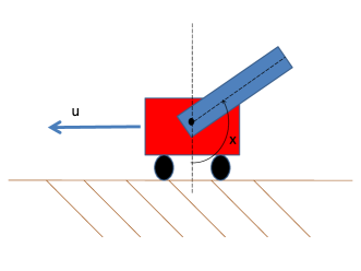
  Figure 3: Inverted pendulum

  

  Figure 4: Sinus complex state space dynamics of the inverted pendulum

  Let us now choose alternatively the complex dynamics

  $$\dot{z}=(1+i)\sin(\frac{z}{2})$$

  with $\lambda_{1}=\frac{1+i}{2}\cos(\frac{z}{2})$. The above is equivalent to

  $$\dot{x} = \sin(\frac{x}{2})\cosh(\frac{y}{2})-\cos(\frac{x}{2})\sinh(\frac{y}{2})$$

  $$\dot{y} = \sin(\frac{x}{2})\cosh(\frac{y}{2})+\cos(\frac{x}{2})\sinh(\frac{y}{2})$$

  whose real second-order plant dynamics is

  $$\ddot{x}=-\frac{1}{2}\cos(x)sinh(y)$$

  with the control input $u=-\frac{1}{2}\sinh(y)$ that stays bounded for bounded $y$. The complex dynamics is illustrated in figure 5. We can see that - as designed - every second upper position is globally stable / unstable.

  

  Figure 5: Sinus half complex state space dynamics of the inverted pendulum

  $\Box$

5 Continuous-time observers

In this section we consider $\forall t\geq 0$ a smooth $n$-th order dynamic system in observability form

$${\bf x}^{(n)}={\bf a}_{1}^{(n-1)}({\bf x},t)+{\bf a}_{2}^{(n-2)}({\bf x},t)+...+{\bf a}_{n}({\bf x},t)$$

with $M$-dimensional measurement ${\bf y}({\bf x},t)$, $N$-dimensional state ${\bf x}$, $N$-dimensional non-linear plant dynamics ${\bf a}_{j}({\bf x},t)$ and time $t$, which is equivalent to

$$\dot{{\bf x}}_{j}={\bf x}_{j+1}+{\bf a}_{j}(\hat{\bf x},t)\ \mbox{for }j=1,...,n$$ (13)

with ${\bf x}_{1}={\bf x}$ and ${\bf x}_{n+1}=0$

Let us now introduce the observer

$$\dot{\hat{{\bf x}}}_{j}=\hat{\bf x}_{j+1}+{\bf a}_{j}(\hat{\bf x},t)+{\bf e}_{j}(\hat{\bf y},t)-{\bf e}_{j}({\bf y},t)\ \mbox{for }j=1,...,n$$

with $\hat{\bf x}_{1}=\hat{\bf x}$ and $\hat{\bf x}_{n+1}=0$ that allows to extend the plant dynamics ${\bf a}_{j}$ with a chosable measurement feedback ${\bf e}_{j}$ in the equivalent $n$-th order observer dynamics

$$\hat{\bf x}^{(n)}=\sum_{j=1}^{n}\left({\bf a}_{j}(\hat{\bf x},t)+{\bf e}_{j}(\hat{\bf y},t)-{\bf e}_{j}({\bf y},t)\right)^{(n-j)}$$ (14)

Let us now generalize the well-known LTI eigenvalue-placement in Jordan form to the placement of the hierachical complex dynamics

$$\dot{\hat{{\bf z}}}_{j}=\int{\bf\Lambda}_{j}(\hat{\bf z}_{j},t)d\hat{\bf z}_{j}+\Re(\hat{\bf z}_{j+1})\ \mbox{for }j=1,...,p-1$$ (15)

with $\Re(\hat{\bf z}_{1})=\hat{\bf x},\hat{\bf z}_{p+1}=0$ and where $p$ is given by $n$ minus the number of complex contraction rate matrices ${\bf\Lambda}_{j}$. Taking the variation of the above implies the time- or state-dependent complex contraction rate matrices ${\bf\Lambda}_{j}$ in

$$\frac{d}{dt}\delta\hat{\bf z}_{j}\ =\ {\bf\Lambda}_{j}(\hat{\bf z}_{j},t)\delta\hat{\bf z}_{j}+\Re(\delta\hat{\bf z}_{j+1})\ \mbox{for }j=1,...,p$$

According to Theorem 4 is the stability of this hierachy given by the definiteness of the Hermitian part of ${\bf\Lambda}_{j}$.

Substituting the $p$ dynamics (15) recursively in each other leads to

Theorem 4

Given the smooth $n$-th order dynamic system in observability form

$${\bf x}^{(n)}={\bf a}_{1}^{(n-1)}({\bf x},t)+{\bf a}_{2}^{(n-2)}({\bf x},t)+...+{\bf a}_{n}({\bf x},t)$$ (16)

with $M$-dimensional measurement ${\bf y}({\bf x},t)$, $N$-dimensional state ${\bf x}$, $N$-dimensional non-linear plant dynamics ${\bf a}_{j}({\bf x},t)$ and time $t$.

An observer

$$\dot{\hat{{\bf x}}}_{j}=\hat{\bf x}_{j+1}+\left({\bf a}_{j}(\hat{\bf x},t)+{\bf e}_{j}(\hat{\bf y},t)-{\bf e}_{j}({\bf y},t)\right)\ \mbox{for }j=1,...,n$$ (17)

with $\hat{\bf x}_{1}=\hat{\bf x}$ and $\hat{\bf x}_{n+1}={\bf 0}$ allows to place with the measurement feedback terms ${\bf e}_{j}$ the time- or state-dependent, integrable, complex contraction rate matrices ${\bf\Lambda}_{j}(\hat{\bf z}_{j},t)$ in the characteristic equation

$$\left(\frac{d}{dt}-\int\Lambda_{p}d\right)\Re...\left(\frac{d}{dt}-\int\Lambda_{1}d\right)\hat{\bf x}={\bf 0}$$ (18)

with $\Re(\hat{\bf z}_{1})=\hat{\bf x},\Re(\hat{\bf z}_{j+1})={\dot{\hat{\bf z}}}_{j}-\int{\bf\Lambda}_{j}(\hat{\bf z}_{j},t)d\hat{\bf z}_{j}$

The definiteness of the Hermitian part of ${\bf\Lambda}_{j}(\hat{\bf z}_{j},t)$ implies global contraction behaviour of the observer state with ${\bf\Lambda}_{j}(\hat{\bf z}_{j},t)$ to the plant state according to Theorem 4.

$p$ is given by $n$ minus the number of complex contraction rate matrices ${\bf\Lambda}_{j}$ and $\Re$ applies to its left-hand term.

This theorem generalizes the extended LTV Luenberger observer design of constant eigenvalues (see e.g. [18], [26] or [38]) to non-linear or state-dependent contraction rates for non-linear, time-varying systems. It provides a systematic observer design technique compared to existing contraction observer designs (see e.g. [1, 27, 39])

Note that the global controller in Theorem 3 that uses the state estimates of the global observer in Theorem 4 satisfies a separation principle. Indeed, subtracting the plant dynamics (13), eventually extended by a control input ${\bf G}({\bf y},t){\bf u}(\hat{\bf x},t)$, from the observer dynamics (17), that is extended by the same control input ${\bf G}({\bf y},t){\bf u}(\hat{\bf x},t)$, leads with $\tilde{\bf x}=\hat{\bf x}-{\bf x}$ and the mid-point theorem to

$$\dot{\tilde{{\bf x}}}_{j}=\tilde{\bf x}_{j+1}+\frac{\partial\left({\bf a}_{n-j}+{\bf e}_{n-j}\right)}{\partial{\bf x}}({\bf\xi},t)\tilde{\bf x}\ \mbox{for }j=1,...,n$$

with $\tilde{\bf x}_{n+1}=0$ and where ${\bf\xi}$ is one point between ${\bf x}$ and $\hat{\bf x}$. We can see that the Jacobian of the error-dynamics of the observer is unchanged. Since $\frac{\partial{\bf u}}{\partial{\bf x}}$ in Theorem 3 is bounded the controller represents a hierarchical system [18]. As a result is the convergence rate of the controller unchanged as well.

Let us now show how a general $Nn$ dimensional plant

$$\dot{\underline{\bf x}}={\bf f}(\underline{\bf x},t)$$

with $N$-dimensional measurement ${\bf y}={\bf x}(\underline{\bf x},t)$ can be transformed to the higher-order observability form (16). A necessary condition is that the mapping

$$\left(\begin{array}[]{c}{\bf y}(\underline{\bf x},t)\\ \vdots\\ {\bf y}^{(n-1)}(\underline{\bf x},t)\end{array}\right)$$

can be inverted to $\underline{\bf x}({\bf y},...,{\bf y}^{(n-1)},t)$ such that we get an explicit dynamics (16)

$${\bf x}^{(n)}={\bf x}^{(n)}(\underline{\bf x}(({\bf x},...,{\bf x}^{(n-1)},t),t)$$

Hence a necessary (but not sufficient) observability condition is that the observability matrix

$${\bf O}=\left(\begin{array}[]{c}L^{o}{\bf c}\\ \vdots\\ L^{n-1}{\bf c}\end{array}\right)$$

with the Lie derivatives [25] $L^{o}{\bf c}=\frac{\partial{\bf y}}{\partial\underline{\bf x}}$ and $L^{j+1}{\bf c}=\frac{\partial{\bf y}^{(j+1)}}{\partial\underline{\bf x}}=L^{j}{\bf c}\frac{\partial{\bf f}}{\partial\underline{\bf x}}+\frac{d}{dt}L^{j}{\bf c}$ has piece-wisely full rank. Note that for LTV systems it is also sufficient.

Let us first consider a linear observer design with time-varying contraction rates.

• Example 5.1

  : Consider the vertical channel dynamics of a navigation system

  $$\ddot{x}=a(t)$$

  with measured altitude $y=x$ and measured vertical acceleration $a(t)$. We want to schedule with Theorem 4 the complex eigenvalues $\lambda_{1}(Ma)$ and $\lambda_{2}(Ma)$ with $Ma(t)$ in the observer (17)

  $$\left(\begin{array}[]{c}\dot{\hat{x}}_{1}\\ \dot{\hat{x}}_{2}\end{array}\right)=\left(\begin{array}[]{c}\hat{x}_{2}\\ a(t)\end{array}\right)+\left(\begin{array}[]{c}e_{1}(Ma)\\ e_{2}(Ma)\end{array}\right)\left(\hat{y}-y\right)$$

  with $\hat{x}=\hat{x}_{1}$ to optimize the vertical channel performance for changing altitude measurement accuracy in sub-, trans- and supersonic. Comparing the second-order observer error dynamics

  $$\ddot{\tilde{x}}=\frac{d}{dt}\left(e_{1}(Ma)\tilde{x}\right)+e_{2}(Ma)\tilde{x}$$

  with $\tilde{x}=\hat{x}-x$ to the characteristic equation (18)

  $$\left(\frac{d}{dt}-\lambda_{2}\right)\left(\frac{d}{dt}-\lambda_{1}\right)\tilde{x}=\ddot{\tilde{x}}-\frac{d}{dt}\left((\lambda_{1}+\lambda_{2})\tilde{x}\right)+(\lambda_{2}\lambda_{1}+\dot{\lambda}_{2})\tilde{x}=0$$

  leads to

  $$e_{1}(Ma) = \lambda_{1}+\lambda_{2}$$

  $$e_{2}(Ma,\dot{Ma}) = -\lambda_{2}\lambda_{1}-\dot{\lambda}_{2}$$

  The difference to standard gain-scheduling techniques (see e.g. [14]) is the term $\dot{\lambda}_{2}$ in the feedback gain computation. Only with this term exponential convergence with the eigenvalues $\lambda_{1}$ and $\lambda_{2}$ is given. $\Box$

Let us consider now observer designs for non-linear systems with time-varying contraction rates:

• Example 5.2

  : Consider the temperature-dependent reaction $A\rightarrow B$ in a closed tank

  $$\frac{d}{dt}\left(\begin{array}[]{c}c_{A}\\ T\end{array}\right)=\left(\begin{array}[]{c}-1\\ -10\end{array}\right)e^{-\frac{E}{T}}c_{A}$$

  with $c_{A}$ the concentration of A, $y=T$ the measured temperature, and $E$ the specific activation energy, where we want to build an observer with designed contraction rates $\lambda_{1}(t),\lambda_{2}(t)<0$.

  This reaction dynamics is equivalent to the following second-order dynamics in temperature

  $$\ddot{T}+\frac{-E}{T^{2}}\dot{T}^{2}=-e^{-\frac{E}{T}}\dot{T}$$

  Letting $x=\int_{o}^{T}e^{\frac{-E}{T}}dT$ yields the plant in observability form

  $$\ddot{x}=\dot{a}_{1}(x)$$

  with $a_{1}(x)=-\int e^{-\frac{E}{\hat{T}(x)}}dx$. Let us design the observer (17) with estimate $\hat{x}=\hat{x}_{1}$

  $$\left(\begin{array}[]{c}\dot{\hat{x}}_{1}\\ \dot{\hat{x}}_{2}\end{array}\right)=\left(\begin{array}[]{c}\hat{x}_{2}+a_{1}\\ 0\end{array}\right)+\left(\begin{array}[]{c}e_{1}(\hat{y})-e_{1}(y)\\ e_{2}(\hat{y})-e_{2}(y)\end{array}\right)$$

  with designed time-varying contraction rates $\lambda_{1}(t),\lambda_{2}(t)<0$. Comparing the equivalent second-order observer dynamics in $\hat{x}$

  $$\ddot{x}-\ddot{\hat{x}}=\frac{d}{dt}\left(a_{1}(\hat{x})-a_{1}(x)+e_{1}(\hat{x}_{1})-e_{1}(x)\right)+e_{2}(\hat{x}_{1})-e_{2}(x)$$

  with the characteristic equation (18)

  $$\left(\frac{d}{dt}-\lambda_{2}\right)\left(\frac{d}{dt}-\lambda_{1}\right)(\hat{x}-x)=0$$

  leads to the non-linear feedback gains

  $$e_{1}(\hat{y})+a_{1}(\hat{y}) = (\lambda_{1}+\lambda_{2})\hat{y}$$

  $$e_{2}(\hat{y}) = -(\lambda_{1}\lambda_{2}+\dot{\lambda}_{2})\hat{y}$$

  $\Box$

The following example gives an explicit equation for the feedback gains of time-dependent contraction rates:

• Example 5.3

  : Consider the $n$-dimensional non-linear system dynamics

  $${\bf x}^{(n)}={\bf a}_{1}^{(n-1)}({\bf x},t)+{\bf a}_{2}^{(n-2)}({\bf x},t)+\ldots+{\bf a}_{n}({\bf x},t)$$

  with non-linear plant dynamics ${\bf a}_{j}({\bf x},t)$ and measurement vector ${\bf y}({\bf x},t)$.

  Comparing the $n$-th order dynamics (14) of the observer (17) to the characteristic equation (18) of real time-varying contraction rates ${\bf\Lambda}_{j}(t)$ implies the feedback gains

  $${\bf e}_{1}(\hat{\bf y},t)+{\bf a}_{1}(\hat{\bf x},t) = \sum_{j=1}^{n}{\bf\Lambda}_{j}\hat{\bf x}$$

  $$\vdots$$

  $${\bf e}_{n}(\hat{\bf y},t)+{\bf a}_{n}(\hat{\bf x},t) = ad_{{\bf\Lambda}_{n}}...(ad_{{\bf\Lambda}_{2}}{\bf\Lambda}_{1})\hat{\bf x}$$

  with $ad_{\bf G}{\bf F}=-{\bf G}{\bf F}-\dot{\bf G}$. $\Box$

Finally let us consider a non-linear observer with state-dependent contraction rates:

• Example 5.4

  : Consider the Van-der-Pol oscillator

  $$\ddot{x}=\dot{a}_{1}(x)+a_{2}(x,t)$$

  with $a_{1}(x)=x-\frac{x^{3}}{3}$ and measured $y=x$. We want to build an observer (17) with estimate $\hat{x}=\hat{x}_{1}$

  $$\left(\begin{array}[]{c}\dot{\hat{x}}_{1}\\ \dot{\hat{x}}_{2}\end{array}\right)=\left(\begin{array}[]{c}\hat{x}_{2}+a_{1}(\hat{x}_{1})\\ a_{2}(\hat{x}_{1},t)\end{array}\right)+\left(\begin{array}[]{c}e_{1}(\hat{y})-e_{1}(y)\\ e_{2}(\hat{y})-e_{2}(y)\end{array}\right)$$

  with designed contraction rates $\lambda_{1}(\hat{x}),\lambda_{2}<0$. Comparing the equivalent second-order observer dynamics in $\hat{x}$

  $$\ddot{x}-\ddot{\hat{x}}=\frac{d}{dt}\left(a_{1}(\hat{x})-a_{1}(x)+e_{1}(\hat{x}_{1})-e_{1}(x)\right)+a_{2}(x,t)-a_{2}(x,t)+e_{2}(\hat{x}_{1})-e_{2}(x)$$

  with the characteristic equation (18)

  $$\left(\frac{d}{dt}-\int\lambda_{2}d\right)\left(\frac{d}{dt}-\int\lambda_{1}d\right)\hat{x} =$$

  $$\ddot{x}-\ddot{\hat{x}}-\frac{d}{dt}\int_{x}^{\hat{x}}(\lambda_{1}+\lambda_{2})d\hat{x}+\lambda_{2}\int_{x}^{\hat{x}}\lambda_{1}d\hat{x} = 0$$

  leads to the non-linear feedback gains

  $$e_{1}(\hat{y})+a_{1}(\hat{y}) = \int(\lambda_{1}+\lambda_{2})d\hat{y}$$

  $$e_{2}(\hat{y},t)+a_{2}(\hat{y},t) = -\lambda_{2}\int\lambda_{1}d\hat{y}$$

  $\Box$

6 Continuous higher-order analysis and robustness

Consider for $t\geq 0$ the $n$-dimensional ($n\geq 1$) system

$${\bf x}^{(n)}={\bf f}({\bf x},...,{\bf x}^{(n-1)},t)$$

with $N$-dimensional position ${\bf x}$.

In Theorem 3 and 4 the characteristic equation of the dynamics above is zero since we use the observer or controller feedback to precisely achieve the characteristic equation. For such a given controller or observer an additional modelling uncertainty ${\bf d}$ may have to be considered on top to the designed characteristic dynamics. This introduces the idea of the existence of a perturbation ${\bf d}$ in the characteristic equation if we analyse a given ODE.

Based on this thought let us approximate this dynamics with the complex, integrable contraction rates ${\bf\Lambda}_{j}({\bf z}_{j},t)$ - that eventually correspond to the designed contraction rates - in the distorted characteristic equation

$$\left(\frac{d}{dt}-\int\Lambda_{p}d\right)\Re...\left(\frac{d}{dt}-\int\Lambda_{1}d\right){\bf x}={\bf d}({\bf z}_{p},..{\bf z}_{1},t)$$

with $\Re({\bf z}_{1})={\bf x}$ and $\Re({\bf z}_{j+1})=\dot{\bf z}_{j}-\int\Lambda_{j}d{\bf z}_{j}$.

Taking the variation of the above we get

$$\delta\dot{\bf z}_{p}-{\bf\Lambda}_{p}\delta{\bf z}_{p}=\frac{\partial{\bf d}}{\partial{\bf z}_{p}}\delta{\bf z}_{p}+\ ...\ +\frac{\partial{\bf d}}{\partial{\bf z}_{1}}\delta{\bf z}_{1}$$

The main idea is to construct in the following an exponential bound on the virtual displacement $\delta{\bf z}_{1}$ over $p$ time-derivatives, rather than over the first time-derivative as in [18].

Let us first bound the higher-order term part by taking the norm of the above

$$\left|\delta\dot{\bf z}_{p}-{\bf\Lambda}_{p}\delta{\bf z}_{p}\right|\leq\left|\frac{\partial{\bf d}}{\partial{\bf z}_{p}}\right||\delta{\bf z}_{p}|+\ldots+\left|\frac{\partial{\bf d}}{\partial{\bf z}_{1}}\right||\delta{\bf z}_{1}|$$ (19)

where now and in the following the norm of a matrix is the largest singular value of that matrix and the norm of a vector is the root of the vector multiplied with its conjungate vector.

Let us now select a real $\eta({\bf z}_{1}(t),...{\bf z}_{p}(t),t)$ that fulfils

$$L^{p}\eta\geq|\frac{\partial{\bf d}}{\partial{\bf z}_{p}}|L^{p}\eta+\ \ldots\ +|\frac{\partial{\bf d}}{\partial{\bf z}_{1}}|$$ (20)

$\forall t\geq 0$ with $L^{j+1}\eta=\dot{L^{j}\eta}+\eta L^{j}\eta\geq 0,L^{o}\eta=1$ and let us bound the initial conditions at $t=0$ with real and constant $K\geq 0$ as

$$|\delta{\bf z}_{j}|\leq K\ L^{j-1}\eta\ e^{\int_{0}^{t}(\eta+\lambda_{max})dt},\ 1\leq j\leq p$$ (21)

where $\lambda_{max}({\bf z}_{1}(t),...{\bf z}_{p}(t),t)$ is the largest eigenvalue of the Hermitian part of all ${\bf\Lambda}_{j}({\bf z}_{j},t)$. Hence with (20) and (21) we can bound (19) at $t=0$ as

$$|\delta\dot{\bf z}_{p}-{\bf\Lambda}_{p}\delta{\bf z}_{p}| \leq K\ e^{\int_{0}^{t}(\eta+\lambda_{max})dt}\left(|\frac{\partial{\bf d}}{\partial{\bf z}_{p}}|L^{p}\eta+\ \ldots\ +|\frac{\partial{\bf d}}{\partial{\bf z}_{1}}|\right)$$ (22)

$$\leq K\ L^{p}\eta\ e^{\int_{0}^{t}(\eta+\lambda_{max})}$$

Theorem 4 on $\delta\dot{\bf z}_{j}={\bf\Lambda}_{j}\delta{\bf z}_{j}+\Re(\delta{\bf z}_{j+1})$ with the bounded distortion (21) and (22) implies at $t=0$

$$|\delta{\bf z}_{j}(t+dt)| \leq |\delta{\bf z}_{j}(t)|+K\ (\lambda_{max}L^{j-1}\eta(t)+L^{j}\eta(t))\ e^{\int_{0}^{t}(\eta+\lambda_{max})}dt$$

$$\leq K\ L^{j-1}\eta(t+dt)\ e^{\int_{0}^{t+dt}(\eta+\lambda_{max})},1\leq j\leq p$$

which implies with complete induction that (21) and (22) hold $\forall t\geq 0$. Using the above this allow to conclude:

Theorem 5

Consider for $t\geq 0$ the $n$-dimensional ($n\geq 1$) system

$${\bf x}^{(n)}={\bf f}({\bf x},...,{\bf x}^{(n-1)},t)$$

with $N$-dimensional position ${\bf x}$.

Let us approximate the above dynamics with the integrable complex contraction rates ${\bf\Lambda}_{j}({\bf z}_{j},t)$ in the distorted characteristic equation

$$\left(\frac{d}{dt}-\int\Lambda_{p}d\right)\Re...\left(\frac{d}{dt}-\int\Lambda_{1}d\right){\bf x}={\bf d}({\bf z}_{p},..{\bf z}_{1},t)\$$ (23)

with $\Re({\bf z}_{1})={\bf x}$ and ${\bf z}_{j+1}=\dot{\bf z}_{j}-\int\Lambda_{j}d{\bf z}_{j}$.

Bounding the effect of the distortion ${\bf d}$ with a real $\eta({\bf z}_{1}(t),...{\bf z}_{p}(t),t)$ that fulfils $\forall t\geq 0$

$$L^{p}\eta^{p}\geq|\frac{\partial{\bf d}}{\partial{\bf z}_{p}}|L^{p}\eta+\ \ldots\ +|\frac{\partial{\bf d}}{\partial{\bf z}_{1}}|$$ (24)

with $L^{j+1}\eta=\dot{L^{j}\eta}+\eta L^{j}\eta\geq 0,L^{o}\eta=1$ and the largest eigenvalue $\lambda_{max}({\bf z}_{1}(t),...{\bf z}_{p}(t),t)$ of the Hermitian part of all ${\bf\Lambda}_{j}({\bf z}_{j},t)$ leads to global contraction behaviour with

$${\bf\Lambda}_{j}({\bf z}_{j},t)+\eta$$ (25)

according to Theorem 4 where initial overshoots are bounded $\forall t\geq 0$ with constant $K>0$ by

$$|\delta{\bf z}_{j}|\leq K\ L^{j-1}\eta(t=0)\ \ e^{\int_{0}^{t}\eta+\lambda_{\max j}dt},\ 1\leq j\leq p$$ (26)

$p$ is given by $n$ minus the number of complex contraction rate matrices ${\bf\Lambda}_{j}$ and $\Re$ applies to its left-hand term.

Interpreting ${\bf\Lambda}_{j}({\bf z}_{j},t)$ as the desired contraction rates in Theorem 3 or 4 allows to bound the potential instabilities which come from modelling uncertainties of the plant. I.e. it allows to prove robustness for modelling uncertainties with a bounded de-stabilizing divergence rate $\eta$. Note that additional time-varying errors in the control input do not affect the contraction behaviour, but the desired trajectory ${\bf x}_{d}(t)$.

If we cannot design ${\bf\Lambda}_{j}({\bf z}_{j},t)$ per feedback then we have to approximate ${\bf\Lambda}_{j}$ to minimize the distortion ${\bf d}$, e.g. by transforming the higher-order system in its reduced form (i.e. a form in which ${\bf f}$ is independent of ${\bf x}^{(n-1)}$). This is illustrated in the following examples:

• Example 6.1

  : Consider the general (a)periodic dynamics

  $$\ddot{\bf x}+\frac{\partial\dot{U}}{\partial{\bf x}}+\frac{\partial^{2}U}{\partial{\bf x}^{2}}_{\min}\dot{\bf x}+\frac{\partial V}{\partial{\bf x}}=0$$

  with potentials $U({\bf x},t),V({\bf x},t)$, $N$-dimensional position ${\bf x}$ and where we assume without los of generality $\frac{\partial^{2}U}{\partial{\bf x}^{2}}_{\min}(t)=\min\left(\frac{\partial^{2}U}{\partial{\bf x}^{2}}\right)$ $\forall{\bf x}$ at a given $t$. The virtual dynamics is

  $$\delta\ddot{\bf x}+\left(\frac{\partial^{2}U}{\partial{\bf x}^{2}}+\frac{\partial^{2}U}{\partial{\bf x}^{2}}_{\min}\right)\delta\dot{\bf x}+\left(\frac{\partial^{2}V}{\partial{\bf x}^{2}}+\frac{\partial^{2}\dot{U}}{\partial{\bf x}^{2}}\right)\delta{\bf x}=0$$

  The distorted characteristic equation (23) is with ${\bf\Lambda}_{1}=-\frac{\partial^{2}U}{\partial{\bf x}^{2}},{\bf\Lambda}_{2}=-\frac{\partial^{2}U}{\partial{\bf x}^{2}}_{\min}$

  $$\left(\frac{d}{dt}-{\bf\Lambda}_{2}\right)\left(\frac{d}{dt}-{\bf\Lambda}_{1}\right)\delta{\bf x}=\left(\frac{\partial^{2}U}{\partial{\bf x}^{2}}_{\min}\frac{\partial^{2}U}{\partial{\bf x}^{2}}-\frac{\partial^{2}V}{\partial{\bf x}^{2}}\right)\delta{\bf x}$$

  The remaining instability $\eta$ in (24) is then given

  $$\dot{\eta}+\eta^{2}\geq\left|\frac{\partial^{2}U}{\partial{\bf x}^{2}}_{\min}\frac{\partial^{2}U}{\partial{\bf x}^{2}}-\frac{\partial^{2}V}{\partial{\bf x}^{2}}\right|$$

  We can hence bound with Theorem 5 the contraction rates with

  $$\frac{\partial^{2}U}{\partial x^{2}}_{min}+\eta\leq\frac{\partial^{2}U}{\partial x^{2}}_{min}+\sqrt{\left|\frac{\partial^{2}U}{\partial{\bf x}^{2}}_{\min}\frac{\partial^{2}U}{\partial{\bf x}^{2}}-\frac{\partial^{2}V}{\partial{\bf x}^{2}}\right|}_{max}$$

  Note that for the scalar case with constant damping this condition is equivalent to require that the complex poles $\frac{\partial^{2}U}{\partial x^{2}}\pm\sqrt{\frac{\partial^{2}U}{\partial x^{2}}^{2}-\frac{\partial^{2}V}{\partial x^{2}}(x,t)}$ lie $\forall x,t$ within the $\pm 45^{o}$ quadrant of the left-half complex plane. $\Box$

• Example 6.2

  : Consider the second-order non-linear system

  $$\ddot{x}+2\dot{x}+\frac{\partial V}{\partial x}=u(t)$$

  with potential energy $V=\ln\cosh(x-x_{d}(t))$, that increases the stabilizing force $-\frac{\partial V}{\partial x}=-\tanh(x-x_{d}(t))$ with the distance to the desired position $x_{d}(t)$. The corresponding variational dynamics is

  $$\delta\ddot{x}+2\delta\dot{x}+\frac{1}{\cosh^{2}(x-x_{d}(t))}\ \delta x=0$$

  Since the LTI poles lie within $\pm 45$ quadrant of the left-half complex plane we can conclude with Example 6.1 on contraction behaviour. $\Box$

7 Discrete-time controllers

In this section we consider $\forall i\geq 0$ a smooth $n$-th order discrete system in controllability form

$${\bf x}^{i+n}={\bf f}({\bf x}^{i},...,{\bf x}^{i+n-1},i)+{\bf G}({\bf x}^{i},...,{\bf x}^{i+n-1},i){\bf u}^{i}$$

with $N$-dimensional position ${\bf x}^{i}$, $M$-dimensional control input ${\bf u}^{i}$ and time index $i$. The controllability conditions under which a general discrete, non-linear, dynamic system can be transformed in the form above is well established for feedback linearizable systems (see e.g. [15, 29]).

Let us now generalize the well-known LTI eigenvalue-placement in Jordan form to the placement of the hierarchical complex dynamics

$${\bf z}_{j}^{i+1}=\int{\bf\Sigma}_{j}({\bf z}_{j}^{i},i)d{\bf z}_{j}^{i}+\Re({\bf z}_{j+1}^{i})\ \mbox{for }j=1,...,p$$ (27)

with $\Re({\bf z}_{1}^{i})={\bf x}^{i},{\bf z}_{p+1}^{i}=0$ and where $p$ is given by $n$ minus the number of complex contraction rate matrices ${\bf\Sigma}_{j}$. Taking the variation of the above implies the time- or state-dependent complex contraction rate matrices ${\bf\Sigma}_{j}$ in

$$\delta{\bf z}_{j}^{i+1}\ =\ {\bf\Sigma}_{j}({\bf z}_{j}^{i},i)\delta{\bf z}_{j}^{i}+\Re(\delta{\bf z}_{j+1}^{i})$$

According to Theorem 8 is the stability of this hierachy given by the singular values of of ${\bf\Sigma}_{j}$.

Substituting the $p$ dynamics (27) recursively in each other leads to:

Theorem 6

Given the smooth $n$-th order system in controllability form

$${\bf x}^{i+n}={\bf f}({\bf x}^{i},...,{\bf x}^{i+n-1},i)+{\bf G}({\bf x}^{i},...,{\bf x}^{i+n-1},i){\bf u}^{i}$$ (28)

with $N$-dimensional position ${\bf x}^{i}$, $M$-dimensional control input ${\bf u}^{i}$ and time index $i$.

A controller ${\bf u}^{i}$ that places the complex, integrable contraction rates ${\bf\Sigma}_{j}({\bf z}_{j}^{i},i)$ in the characteristic equation

$$\left({}^{(+1)}-\int{\bf\Sigma}_{p}d\right)\Re...\left({}^{(+1)}-\int{\bf\Sigma}_{1}d\right){\bf x}^{i}={\bf 0}$$ (29)

with $\Re({\bf z}_{1}^{i})={\bf x}^{i},\Re({\bf z}_{j+1}^{i})={\bf z}_{j}^{i+1}-\int{\bf\Sigma}_{j}({\bf z}_{j}^{i},i)d{\bf z}_{j}^{i}$ implies global contraction behaviour with ${\bf\Sigma}_{j}({\bf z}_{j}^{i},i)$ according to Theorem 8.

$p$ is here given by $n$ minus the number of complex contraction rate matrices ${\bf\Sigma}_{j}$ and $\Re$ applies to its left-hand term. The open integral $\int$ implies a time-varying integration constant that can be chosen to shape a desired trajectory in the flow field without affecting the contraction behaviour.

The generalization to standard feedback linearization methods (see e.g. [15, 29]) is that we can choose state- or time-dependent contraction rates ${\bf\Sigma}_{j}({\bf z}_{j}^{i},i)$ to simplify ${\bf u}^{i}$, to handle only piece-wisely controllable systems or simply to achieve a state- or time-dependent system performance.

In contrast to well-known gain-scheduling techniques (see e.g. [14]), who also intend to achieve state-dependent stability behaviour, we can analytically proof global contraction behaviour with ${\bf\Sigma}_{j}({\bf z}_{j}^{i},i)$. Analytic robustness guarantees to modelling uncertainties are given in section 9.

Note that (29) can be modally solved as

$$\delta{\bf z}_{j}^{i+1}=\sum_{l=0}^{i}\left(\Phi(l+1,i)\Re(\delta{\bf z}_{j+1}^{l})\right)+\Phi(0,i)\delta{\bf z}_{j}^{o}$$

with the transition matrix $\Phi(0,i)$ in equation (1) which can be analytically over/under-bounded with Theorem 8. This extends the well-established LTI convolution principle to state- and time-dependent contraction rates.

Let us first consider LTV systems before we go to real and then complex non-linear systems:

• Example 7.1

  : Consider the second-order real, time-varying dynamics

  $${\bf x}^{i+2}+{\bf D}(i){\bf x}^{i+1}+{\bf K}(i){\bf x}^{i}={\bf u}(i)$$

  Real contraction rates ${\bf\Sigma}_{1}(i)$ and ${\bf\Sigma}_{2}(i)$ imply with the characteristic equation (29) in Theorem 6

  $${\bf D}(i) = -{\bf\Sigma}_{1}^{(+1)}-{\bf\Sigma}_{2}$$

  $${\bf K}(i) = {\bf\Sigma}_{2}{\bf\Sigma}_{1}$$

  A complex contraction rate ${\bf\Sigma}_{1}(i)$ in

  $$\delta{\bf z}_{1}^{i+1}={\bf\Sigma}_{1}(i)\delta{\bf z}_{1}^{i}$$

  implies the real dynamics

  $$\delta{\bf x}^{i+1} = {\bf Re}^{i}\delta{\bf x}^{i}+{\bf Im}^{i}\delta{\bf y}^{i}$$

  $$\delta{\bf y}^{i+1} = -{\bf Im}^{i}\delta{\bf x}^{i}+{\bf Re}^{i}\delta{\bf y}^{i}$$

  with $\delta{\bf x}^{i}=\Re(\delta{\bf z}_{1}^{i})$, $\delta{\bf y}^{i}=\Im(\delta{\bf z}_{1}^{i})$, ${\bf Re}=\Re({\bf\Sigma}_{1})$ and ${\bf Im}=\Im({\bf\Sigma}_{1})$. Rewriting the above as second-order dynamics in $\delta{\bf x}^{i}$ implies

  $${\bf D}(i) = -{\bf Re}^{(+1)}-{\bf Im}^{(+1)}{\bf Re}{\bf Im}^{-1}$$

  $${\bf K}(i) = {\bf Im}^{(+1)}{\bf Re}{\bf Im}^{-1}{\bf Re}+{\bf Im}^{(+1)}{\bf Im}$$

  Note that only the change in the time-indices makes this analytic stability result correct in comparison to a standard LTI approximation of the LTV system. $\Box$

Let us now consider the placement of real and state-dependent contraction rates.

• Example 7.2

  : Consider the second-order discrete system

  $$x^{i+2}=f^{i}(x^{i+1},x^{i},i)+u^{i}$$

  with position $x^{i}$ and control input $u^{i}$.

  Let us now schedule $\sigma_{1}(z_{1}^{i},i)$ and $\sigma_{2}(z_{2}^{i},i)$ with $z_{1}^{i}=x^{i},z_{2}^{i}=z_{1}^{i+1}-\int\sigma_{1}dz_{1}^{i}$ in the characteristic equation (29) of Theorem 6

  $$\left({}^{(+1)}-\int\sigma_{2}d\right)\left({}^{(+1)}-\int\sigma_{1}d\right)x^{i}=0$$

  This is equivalent to require the control input $u^{i}$ in

  $$x^{i+2} = f^{i}(x^{i+1},x^{i},i)+u^{i}$$

  $$= -\int\sigma_{1}(z_{1}^{i+1},i+1)dz_{1}^{i+1}+\int\sigma_{2}(z_{2}^{i},i)dz_{2}^{i}$$

  where the time-varying integration constant can be chosen to achieve tracking-behaviour of the controller to a desired trajectory. $\Box$

Finally let us consider the placement of complex and state-dependent contraction rates.

• Example 7.3

  : Let us now schedule non-linear complex contraction rates for a second-order discrete system by requiring the first-order complex dynamics

  $$z^{i+1}=\frac{1}{2}(z^{i})^{2}+u_{d}^{i}(i)$$ (30)

  with complex contraction rate $\sigma=|z^{i}|$. In principle any differentiable complex function can be used here to schedule the state-dependent complex contraction rates as we want.

  The convergence rate of an arbitrary trajectory $z_{1}$ to another trajectory $z_{2}$ is

  $$\frac{s^{i+1}}{s^{i}}=\frac{\left({\bf z}_{1}^{i+1}-{\bf z}_{2}^{i+1}\right)^{\ast T}\left({\bf z}_{1}^{i+1}-{\bf z}_{2}^{i+1}\right)}{\left({\bf z}_{1}^{i}-{\bf z}_{2}^{i}\right)^{\ast T}\left({\bf z}_{1}^{i}-{\bf z}_{2}^{i}\right)}=\frac{1}{2}|{\bf z}_{1}^{i+1}+{\bf z}_{2}^{i+1}|$$

  according to (8) Theorem 8. This region of convergence is naturally larger then the contraction region $\sigma\leq 1$.

  The complex dynamics is illustrated in figure 6. We can see that $|\sigma|$ increases from the stable origin. We find excactly two equilibrium points at $z_{1}^{i}=0$ and $z_{2}^{i}=2$ with constant distance $\frac{s^{i+1}}{s^{i}}=1$.

  

  Figure 6: Quadratic complex discrete state space dynamics

  The complex dynamics is with $x^{i}=\Re(z^{i})$ and $y^{i}=\Im(z^{i})$ equivalent to

  $$x^{i+1} = \frac{1}{2}(x^{i})^{2}-\frac{1}{2}(y^{i})^{2}+u_{d}^{i}$$

  $$y^{i+1} = x^{i}y^{i}$$

  with corresponding Jacobian

  $$\left(\begin{array}[]{cc}x^{i}&-y^{i}\\ y^{i}&x^{i}\end{array}\right)$$

  that is contracting with $\sigma=\sqrt{(x^{i})^{2}+(y^{i})^{2}}$.

  Hence the corresponding real second-order plant dynamics to (30) is

  $$x^{i+2}=\frac{1}{2}(x^{i+1})^{2}+x^{i+1}(x^{i})^{2}-\frac{1}{2}(x^{i})^{4}-(x^{i})^{2}u^{i}+u^{i+1}$$

  to which the same convergence results apply. $\Box$

8 Discrete-time observers

In this section we consider $\forall i\geq 0$ a smooth $n$-th order dynamic system in observability form

$${\bf x}^{i+n}={\bf a}_{1}^{(+n-1)}({\bf x}^{i},i)+{\bf a}_{2}^{(+n-2)}({\bf x}^{i},i)+...+{\bf a}_{n}({\bf x}^{i},i)$$

with $M$-dimensional measurement ${\bf y}^{i}({\bf x}^{i},i)$, $N$-dimensional state ${\bf x}^{i}$, $N$-dimensional non-linear plant dynamics ${\bf a}_{j}({\bf x}^{i},i)$ and time index $i$, which is equivalent to

$${\bf x}^{i+1}_{j}={\bf x}_{j+1}^{i}+{\bf a}_{j}({\bf x}^{i},i)\ \mbox{for }j=1,...,n$$ (31)

with ${\bf x}^{i}_{1}={\bf x}^{i}$ and $\hat{\bf x}^{i}_{n+1}={\bf 0}$.

Let us now introduce the observer

$$\hat{\bf x}^{i+1}_{j}=\hat{\bf x}_{j+1}^{i}+{\bf a}_{j}(\hat{\bf x}^{i},i)+{\bf e}_{j}(\hat{\bf y}^{i},i)-{\bf e}_{j}({\bf y}^{i},i)\ \mbox{for }j=1,...,n$$

with $\hat{\bf x}^{i}_{1}=\hat{\bf x}^{i}$ and $\hat{\bf x}^{i}_{n+1}={\bf 0}$ that allows to extend the plant dynamics ${\bf a}_{j}$ with a chosable measurement feedback ${\bf e}_{j}$ in the equivalent $n$-th order observer dynamics

$$\hat{\bf x}^{i+n}=\sum_{j=1}^{n}\left({\bf a}_{j}(\hat{\bf x}^{i},i)+{\bf e}_{j}(\hat{\bf y}^{i},i)-{\bf e}_{j}({\bf y}^{i},i)\right)^{(+n-j)}$$ (32)

Let us now generalize the well-known LTI eigenvalue-placment in Jordan form to the placement of the hieracial complex dynamics

$$\hat{\bf z}_{j}^{i+1}=\int{\bf\Lambda}_{j}(\hat{\bf z}_{j}^{i},i)d\hat{\bf z}_{j}^{i}+\Re(\hat{\bf z}_{j+1}^{i})\ \mbox{for }j=1,...,p-1$$ (33)

with $\Re(\hat{\bf z}_{1}^{i})=\hat{\bf x}^{i},\hat{\bf z}_{p+1}^{i}=0$ and where $p$ is given by $n$ minus the number of complex contraction rate matrices ${\bf\Sigma}_{j}$. Taking the variation of the above implies the time-or state-dependent complex contraction rate matrices ${\bf\Sigma}_{j}^{i}$ in

$$\delta\hat{\bf z}_{j}^{i+1}\ =\ {\bf\Sigma}_{j}^{i}(\hat{\bf z}_{j}^{i},i)\delta\hat{\bf z}_{j}^{i}+\delta\hat{\bf z}_{j+1}^{i}\ \mbox{for }j=1,...,p$$

According to Theorem 8 is the stability of this hierachy given by the largest singular value of ${\bf\Sigma}_{j}$.

Substituting the $p$ dynamics (33) recursively in each other leads with to

Theorem 7

Given the smooth $n$-th order dynamic system in observability form

$${\bf x}^{i+n}={\bf a}_{1}^{(+n-1)}({\bf x}^{i},i)+{\bf a}_{2}^{(+n-2)}({\bf x}^{i},i)+...+{\bf a}_{n}({\bf x}^{i},i)$$ (34)

with $M$-dimensional measurement ${\bf y}({\bf x}^{i},i)$ of the $N$-dimensional state ${\bf x}^{i}$, $N$-dimensional non-linear plant dynamics ${\bf a}_{j}({\bf x}^{i},i)$ and time index $i$.

An observer

$$\hat{\bf x}^{i+1}_{j}=\hat{\bf x}_{j+1}^{i}+{\bf a}_{j}(\hat{\bf x}^{i},i)+{\bf e}_{j}(\hat{\bf y}^{i},i)-{\bf e}_{j}({\bf y}^{i},i)\ \mbox{for }j=1,...,n$$ (35)

with $\hat{\bf x}_{1}^{i}=\hat{\bf x}^{i}=\Re(\hat{\bf z}_{1})$ and $\hat{\bf x}^{i}_{n+1}={\bf 0}$ allows to place with the measurement feedback terms ${\bf e}_{j}$ the time- or state-dependent, integrable, complex contraction rate matrices ${\bf\Sigma}_{j}(\hat{\bf z}_{j}^{i},i)$ in the characteristic equation

$$\left({}^{(+1)}-\int\Sigma_{p}d\right)\Re...\left({}^{(+1)}-\int\Sigma_{1}d\right)\hat{\bf x}^{i}={\bf 0}$$ (36)

with $\Re(\hat{\bf z}_{1}^{i})=\hat{\bf x}^{i},\Re(\hat{\bf z}_{j+1}^{i})=\hat{\bf z}_{j}^{i+1}-\int{\bf\Lambda}_{j}(\hat{\bf z}_{j}^{i},i)d\hat{\bf z}_{j}^{i}$.

The largest singular value of ${\bf\Sigma}_{j}^{i}(\hat{\bf z}_{j}^{i},i)$ implies global contraction behavior of the observer state with ${\bf\Sigma}_{j}^{i}(\hat{\bf z}_{j}^{i},i)$ to the plant state according to Theorem 8.

$p$ is given by $n$ minus the number of complex contraction rate matrices ${\bf\Sigma}_{j}^{i}$ and $\Re$ applies to its left-hand term.

This theorem generalizes the extended LTV Luenberger observer design of constant eigenvalues (see e.g. [18], [26] or [38]) to non-linear or state-dependent contraction rates for non-linear, time-varying systems.

Note that the global controller in Theorem 6 that uses the state estimates of the global observer in Theorem 7 satisfies a separation principle. Indeed, subtracting the plant dynamics (31), eventually extended by a control input ${\bf G}({\bf y}^{i},i){\bf u}^{i}(\hat{\bf x}^{i},i)$, from the observer dynamics (35), that is extended by the same control input ${\bf G}({\bf y}^{i},i){\bf u}^{i}(\hat{\bf x}^{i},i)$, leads with $\tilde{\bf x}^{i}=\hat{\bf x}^{i}-{\bf x}^{i}$ and the mid-point theorem to

$$\tilde{{\bf x}}_{j}^{i+1}=\tilde{\bf x}_{j+1}^{i}-\frac{\partial\left({\bf a}_{j}+{\bf e}_{j}\right)}{\partial{\bf x}^{i}}({\bf\xi},i)\tilde{\bf x}^{i}\ \mbox{for }j=1,...,n$$

with $\tilde{\bf x}_{n+1}^{i}=0$ and where ${\bf\xi}$ is one point between ${\bf x}^{i}$ and $\hat{\bf x}^{i}$. We can see that the Jacobian of the error-dynamics of the observer is unchanged. Since $\frac{\partial{\bf u}^{i}}{\partial{\bf x}^{i}}$ in Theorem 3 is bounded the controller represents a hierarchical system [18]. As a result is the convergence rate of the controller unchanged as well.

Let us now show how a general $Nn$ dimensional plant

$$\underline{\bf x}^{i+1}={\bf f}(\underline{\bf x}^{i},i)$$

with $N$-dimensional measurement ${\bf y}^{i}={\bf x}^{i}(\underline{\bf x}^{i},i)$ can be transformed to the higher-order observability form (34). A necessary condition is that the mapping

$$\left(\begin{array}[]{c}{\bf y}^{i}(\underline{\bf x}^{i},i)\\ \vdots\\ {\bf y}^{i+n-1}(\underline{\bf x}^{i},i)\end{array}\right)$$

can be inverted to $\underline{\bf x}^{i}({\bf y}^{i},...,{\bf y}^{i+n-1},i)$ such that we get an explict dynamics (34)

$${\bf x}^{i+n}={\bf x}^{i+n}(\underline{\bf x}^{i}({\bf y}^{i},...,{\bf y}^{i+n-1},i),i)$$

Hence a necessary (but not sufficientI) observability condition is that the observability matrix

$${\bf 0}=\left(\begin{array}[]{c}L^{o}{\bf c}\\ \vdots\\ L^{n-1}{\bf c}\end{array}\right)$$

with the Lie derivatives [25] $L^{o}{\bf c}=\frac{\partial{\bf y}^{i}}{\partial\underline{\bf x}^{i}}$ and $L^{j+1}{\bf c}=\frac{\partial{\bf y}^{i+j+1}}{\partial\underline{\bf x}^{i}}=L^{j}{\bf c}^{(+1)}\frac{\partial{\bf f}}{\partial\underline{\bf x}}^{(+j)}$ has piece-wisely full rank. Note that for LTV systems it is also sufficient.

Let us now consider the observer design of a specific non-linear problem before we go to the general non-linear case:

• Example 8.1

  : Consider the logistic map dynamics

  $$b^{i+1}=c^{i}\ b^{i}\ (1-b^{i})$$

  with measured state $y^{i}=b^{i}$ and unknown constant gain $c^{i}$. We can rewrite the above as second-order system

  $$b^{i+2}=\frac{b^{i+1}\ b^{i+1}\ (1-b^{i+1})}{b^{i}(1-b^{i})}$$

  Introducing the complex state $x^{i}=\ln b^{i}$ we get

  $$x^{i+2}=a_{1}^{(+1)}+a_{2}$$

  with $a_{1}=\ln(b^{i}b^{i}(1-b^{i}))$ and $a_{2}=-\ln(b^{i}(1-b^{i}))$.

  We want to build an observer (35) with estimate $\hat{x}^{i}=\hat{x}_{1}^{i}$

  $$\left(\begin{array}[]{c}\hat{x}_{1}^{i+1}\\ \hat{x}_{2}^{i+1}\end{array}\right)=\left(\begin{array}[]{c}\hat{x}_{2}^{i}+a_{1}(\hat{x}^{i})\\ a_{2}(\hat{x}^{i})\end{array}\right)+\left(\begin{array}[]{c}e_{1}(\hat{y}^{i})-e_{1}(y^{i})\\ e_{2}(\hat{y}^{i})-e_{2}(y^{i})\end{array}\right)$$

  with designed constant contraction rates $|\sigma_{1}|,|\sigma_{2}|<1$. Comparing the equivalent second-order dynamics (32) in $\hat{x}^{i}$

  $$\hat{x}^{i+2}-x^{i+2}=\left(a_{1}(\hat{x}^{i})-a_{1}(x^{i})+e_{1}(\hat{x})-e_{1}(x^{i})\right)^{(+1)}+\left(a_{2}(\hat{x}^{i})-a_{2}(x^{i})+e_{1}(\hat{x})-e_{1}(x^{i})\right)$$

  with the characteristic equation (36)

  $$\left({}^{(+1)}-\int\sigma_{2}d\right)\left({}^{(+1)}-\int\sigma_{1}d\right)(\hat{x}^{i}-x^{i})=0$$

  leads to the non-linear feedback

  $$e_{1}(\hat{y}^{i})+a_{1}(\hat{y}^{i}) = (\sigma_{1}+\sigma_{2})\hat{y}^{i}$$

  $$e_{2}(\hat{y}^{i})+a_{2}(\hat{y}^{i}) = -\sigma_{1}\sigma_{2}\hat{y}^{i}$$

  Note that the observer can be transformed back to the real coordinates $\hat{b}_{1}^{i}=e^{\hat{x}_{1}^{i}},\hat{b}_{2}^{i}=e^{\hat{x}_{2}^{i}}$ as

  $$\left(\begin{array}[]{c}\hat{b}_{1}^{i+1}\\ \hat{b}_{2}^{i+1}\end{array}\right)=\left(\begin{array}[]{c}\hat{b}_{2}^{i}\ \hat{b}^{i}_{1}\hat{b}^{i}_{1}(1-\hat{b}^{i}_{1})\ e^{e_{1}(\hat{y}^{i})-e_{1}(y^{i})}\\ \frac{1}{b^{i}_{1}(1-\hat{b}^{i}_{1})}e^{e_{2}(\hat{y}^{i})-e_{2}(y^{i})}\end{array}\right)$$

  such that we can compute $\hat{b}^{i}=\hat{b}_{1}^{i}$ and the estimated unknown gain as

  $$\hat{c}^{i}=-\frac{\hat{b}^{i+1}_{1}}{\hat{b}^{i}_{1}\ (1-\hat{b}^{i}_{1})}=\hat{b}_{2}^{i}\ \hat{b}^{i}_{1}e^{e_{1}(\hat{y}^{i})-e_{1}(y^{i})}$$

  $\Box$

The following example gives an explicit equation for the feedback gains to achieve time-dependent contraction rates:

• Example 8.2

  : Consider the $n$-dimensional non-linear system dynamics

  $${\bf x}^{i+n}={\bf a}_{1}^{(+n-1)}({\bf x}^{i},i)+{\bf a}_{2}^{(+n-2)}+...+{\bf a}_{n}({\bf x}^{i},i)$$

  with non-linear plant dynamics ${\bf a}_{j}({\bf x}^{i},i)$ and measurement ${\bf y}^{i}(x^{i},i)$.

  Comparing the $n$-th order dynamics (32) of the observer (35) to the characteristic equation (36) of real time-varying contraction rates ${\bf\Sigma}_{j}(i)$ implies the feedback gains

  $${\bf e}_{n}(\hat{\bf y}^{i},i)+\hat{\bf a}_{n}(\hat{\bf x}^{i},i) = \Pi_{j=n}^{1}{\bf\Sigma}_{j}\hat{\bf x}^{i}$$

  $$\vdots$$

  $${\bf e}_{1}(\hat{\bf y}^{i},i)+\hat{\bf a}_{1}(\hat{\bf x}^{i},i) = \sum_{j=1}^{n}{\bf\Sigma}_{j}^{(-j+1)}\hat{\bf x}^{i}$$

  $\Box$

9 Discrete higher-order analysis and robustness

Consider for $i\geq 0$ the $n$-th dimensional ($n\geq 1$) system

$${\bf x}^{i+n}={\bf f}({\bf x}^{i},...,{\bf x}^{i+n-1},i)$$

with $N$-dimensional position ${\bf x}^{i}$.

In Theorem 6 and 7 the characteristic equation of the dynamics above is zero since we use the observer or controller feedback to precisely achieve the characteristic equation. For such a given controller or observer an additional modelling uncertainty ${\bf d}$ may have to be considered on top to the designed characteristic dynamics. This introduces the idea of the existence of a perturbation ${\bf d}$ in the characteristic equation if we analyse a given ODE.

Based on this thought let us approximate this dynamics with the complex, integrable contraction rates ${\bf\Sigma}_{j}^{i}({\bf z}_{j}^{i},i)$ - that eventually correspond to the designed contraction rates - in the distorted characteristic equation

$$\left({}^{(+1)}-\int{\bf\Sigma}_{p}d\right)\Re...\left({}^{(+1)}-\int{\bf\Sigma}_{1}d\right){\bf x}^{i}={\bf d}({\bf z}_{p}^{i},...{\bf z}_{1}^{i},i)$$

with $\Re({\bf z}_{1})={\bf x}$ and $\Re({\bf z}_{j+1}^{i})={\bf z}_{j}^{i+1}-\int{\bf\Sigma}_{j}({\bf z}_{j}^{i},i)d{\bf z}_{j}^{i}$. For a controller or observer of Theorem 6 or 7 ${\bf d}$ may represent the modelling uncertainities of the system.

Taking the variation of the above we get

$$\delta{\bf z}_{p}^{i+1}-{\bf\Sigma}_{p}\delta{\bf z}_{p}^{i}=\frac{\partial{\bf d}}{\partial{\bf z}_{p}^{i}}\delta{\bf z}_{p}^{i}+\ ...\ +\frac{\partial{\bf d}}{\partial{\bf z}_{1}^{i}}\delta{\bf z}_{1}^{i}$$

The main idea is to construct an exponential bound on the virtual displacement $\delta{\bf x}^{i}$ over $p$ time-steps, rather than over a single time-step as in [18].

Let us first bound the higher-order term by taking the norm of the above

$$|\delta{\bf z}_{p}^{i+1}-{\bf\Sigma}_{p}\delta{\bf x}_{p}^{i}|\leq|\frac{\partial{\bf d}}{\partial{\bf z}_{p}^{i}}||\delta{\bf z}_{p}^{i}|+\ldots+|\frac{\partial{\bf d}}{\partial{\bf z}_{1}^{i}}||\delta{\bf z}_{1}^{i}|$$ (37)

where now and in the following the norm of a matrix is the largest singular value of that matrix and the norm of a vector is the root of the vector multiplied with its conjungate vector.

Let us now select a real $\eta^{i}({\bf z}_{1}^{i},...,{\bf z}_{p}^{i},i)\geq 0$ that fulfils

$$\eta^{i+p-1}...\eta^{i}\geq|\frac{\partial{\bf d}}{\partial{\bf z}_{p}^{i}}|\eta^{i+p-2}...\eta^{i}+\ \ldots\ +|\frac{\partial{\bf d}}{\partial{\bf z}_{1}^{i}}|$$ (38)

$\forall i\geq 0$. Let us bound the initial conditions at $i=0$ with real and constant $K\geq 0$ as

$$|\delta{\bf z}_{j}^{i}|\leq K\ \eta^{i+j-2}...\eta^{i}\ \Pi_{k=0}^{i-1}(\eta^{k}+\sigma_{max}^{k}),\ 1\leq j\leq p$$ (39)

where $\sigma_{max}^{i}({\bf z}_{1}^{i},...,{\bf z}_{p}^{i},i)$ is the largest singular value of all ${\bf\Sigma}_{j}({\bf z}_{j}^{i},i)$. Hence with (38) and (39) we can bound (37) at $i=0$ as

$$|\delta{\bf z}_{p}^{i+1}-{\bf\Sigma}_{p}\delta{\bf z}_{n-1}^{i}| \leq K\ \Pi_{k=0}^{i-1}(\eta^{k}+\sigma_{max}^{k})\left(|\frac{\partial{\bf d}}{\partial{\bf z}_{p}^{i}}|\eta^{i+p-2}...\eta^{i}+\ \ldots\ +|\frac{\partial{\bf d}}{\partial{\bf z}_{1}^{i}}|\right)$$ (40)

$$\leq K\ \eta^{i+p-1}...\eta^{i}\ \Pi_{k=0}^{i-1}(\eta^{k}+\sigma_{max}^{k})$$

Theorem 8 on $\delta{\bf z}_{j}^{i+1}=\Lambda_{j}+\Re({\bf z}_{j+1})$ with the bounded distortion (39) and (40) implies at $i=1$

$$|\delta{\bf z}^{i+1}_{j}| \leq \sigma_{max}^{i}|\delta{\bf z}^{i}_{j}|+K\ \eta^{i+j-1}...\eta^{i}\ \Pi_{k=0}^{i-1}(\eta^{k}+\sigma_{max}^{k})$$

$$\leq K\ \eta^{i+j-1}...\eta^{i+1}\ \Pi_{k=0}^{i}(\eta^{k}+\sigma_{max}^{k}),1\leq j\leq p$$

which implies with complete induction that (39) and (40) hold $\forall i\geq 0$.

Using the above this allows to conclude:

Theorem 8

Consider for $i\geq 0$ the $n$-dimensional ($n\geq 1$) system

$${\bf x}^{i+n}={\bf f}^{i}({\bf x}^{i},...,{\bf x}^{i+n-1},i)$$

with $N$-dimensional position ${\bf x}^{i}$ at time $i$.

Let us approximate the above dynamics with the integrable, complex contraction rates ${\bf\Sigma}_{j}({\bf z}_{j}^{i},i)$ in the distorted characteristic equation

$$\left({}^{(+1)}-\int{\bf\Sigma}_{p}d\right)\Re...\left({}^{(+1)}-\int{\bf\Sigma}_{1}d\right){\bf x}^{i}={\bf d}({\bf z}_{p}^{i},...{\bf z}_{1}^{i},i)$$ (41)

with $\Re({\bf z}_{1}^{i})={\bf x}^{i}$ and $\Re({\bf z}_{j+1}^{i})={\bf z}_{j}^{i+1}-\int{\bf\Sigma}_{j}({\bf z}_{j}^{i},i)d{\bf z}_{j}^{i}$.

Bounding the effect of the distortion ${\bf d}$ with a real $\eta^{i}({\bf z}_{1}^{i},...,{\bf z}_{p}^{i},i)\geq 0$ that fulfils $\forall i\geq 0$

$$\eta^{i+n-1}...\eta^{i}\geq|\frac{\partial{\bf d}}{\partial{\bf z}_{p}}|\eta^{i+n-2}...\eta^{i}+\ \ldots\ +|\frac{\partial{\bf d}}{\partial{\bf z}_{1}}|$$ (42)

and the largest singular value $\sigma_{max}^{i}({\bf z}_{1}^{i},...,{\bf z}_{p}^{i},i)$ of all ${\bf\Sigma}_{j}({\bf z}_{j}^{i},i)$ leads to global contraction behaviour with

$${\bf\Sigma}_{j}({\bf z}_{j}^{i},i)+\eta^{i}$$ (43)

according to Theorem 8 where initial overshoots are bounded $\forall i\geq 0$ with constant $K>0$ by

$$|\delta{\bf z}_{j}^{i}|\leq K\ \eta^{j-1}...\eta^{o}(i=0)\ \ (\eta^{i-1}+\sigma_{\max j}^{i-1})...(\eta^{o}+\sigma_{\max j}^{0}),\ 1\leq j\leq p$$ (44)

$p$ is given by $n$ minus the number of complex contraction rate matrices ${\bf\Sigma}_{j}$ and $\Re$ applies to its left-hand term.

Figure 7 illustrates the exponential bound (39) which allows short-term over-shoots but implies exponential convergence on the long-term.

Figure 7: Bound on $\delta z_{j}^{i}$ over $i$

Interpreting ${\bf\Sigma}_{j}$ as the desired contraction rates in Theorem 6 or 7 allows to bound the potential instabilities which come from modelling uncertainties of the plant. I.e. it allows to prove robustness for modelling uncertainties with a bounded de-stabilizing divergence rate $\eta^{i}$. Note that additional time-varying errors in the control input do not affect the contraction behaviour, but the desired trajectory ${\bf x}_{d}^{i}(i)$.

If we cannot design ${\bf\Sigma}_{j}({\bf z}_{j}^{i},i)$ per feedback then we have to approximate ${\bf\Sigma}_{j}$ to minimize the distortion ${\bf d}$, e.g. by transforming the higher-order system in its reduced form (i.e. a form in which ${\bf f}$ is independent of ${\bf x}^{i+n-1}$). This is illustrated in the following examples:

• Example 9.1

  : In economics, consider the price dynamics

  $${\bf n}^{i+1} = {\bf f}({\bf p}^{i},i)$$

  $${\bf p}^{i+1} = {\bf g}({\bf n}^{i},i)$$

  with ${\bf n}^{i}$ the number of sold products at time $i$ and corresponding price ${\bf p}^{i}$.

  The first line above defines the customer demand as a reaction to a given price. The second line defines the price, given by the production cost under competition, as a reaction to the number of sold items. The dynamics above corresponds to the second-order economic growth cycle dynamics

  $${\bf n}^{i+2}={\bf f}\left({\bf g}({\bf n}^{i},i)\right)$$

  Contraction behaviour of this economic behaviour with contraction rate $\eta^{i}$ can then be concluded with equation (42) in Theorem 8 for ${\bf\Sigma}_{1}={\bf\Sigma}_{2}={\bf 0}$

  $$\eta^{i+1}\eta^{i}\geq\left|\frac{\partial{\bf f}}{\partial{\bf p}^{i}}\frac{\partial{\bf g}}{\partial{\bf n}^{i}}\right|$$ (45)

  That means we get stable (contraction) behaviour if the product of customer demand sensitivity to price and production cost sensitivity to number of sold items has singular values less than 1. We get unstable (diverging) behaviour for the opposite case.

  Note that this result even holds when no precise model of the sensitivity is known, which is usually the case in economic or game situations. Whereas the above is well known for LTI economic models we can see that the economic behaviour is unchanged for a non-linear, time-varying economic environment.

  The above also corresponds to a game situation (see e.g. [34] or [7]) between two players with strategic action ${\bf p}^{i}$ and ${\bf n}^{i}$. Both players optimize their reaction ${\bf g}$ and ${\bf f}$ with respect to the opponent’s action. We can then again conclude for (45) to global contraction behaviour to a unique time-dependent trajectory (in the autonomous case, the Nash equilibrium). $\Box$

• Example 9.2

  : Consider the general dynamics

  $${\bf x}^{i+2}+\frac{\partial U}{\partial{\bf x}^{i}}^{(+1)}+\frac{\partial^{2}U}{\partial({\bf x}^{i})^{2}}_{\min}{\bf x}^{i+1}+\frac{\partial V}{\partial{\bf x}^{i}}={\bf 0}$$

  with potentials $U({\bf x}^{i},i),V({\bf x}^{i},i)$, $N$-dimensional position ${\bf x}^{i}$ and where we assume without loss of generality that the singular values of $\frac{\partial^{2}U}{\partial({\bf x}^{i})^{2}}_{\min}$ correspond $\forall{\bf x}^{i}$ at a given $i$ to the minimal singular values of $\frac{\partial^{2}U}{\partial({\bf x}^{i})^{2}}$. The virtual dynamics is

  $$\delta{\bf x}^{i+2}+\left(\frac{\partial^{2}U}{\partial({\bf x}^{i})^{2}}^{(+1)}+\frac{\partial^{2}U}{\partial({\bf x}^{i})^{2}}_{\min}\right)\delta{\bf x}^{i+1}+\frac{\partial^{2}V}{\partial({\bf x}^{i})^{2}}\delta{\bf x}^{i}={\bf 0}$$

  The distorted characteristic equation (41) is with ${\bf\Sigma}_{1}=-\frac{\partial^{2}U}{\partial({\bf x}^{i})^{2}}$, ${\bf\Sigma}_{2}=-\frac{\partial^{2}U}{\partial({\bf x}^{i})^{2}}_{\min}$

  $$\left({}^{(+1)}-\Sigma_{2}\right)...\left({}^{(+1)}-\Sigma_{1}\right)\delta{\bf x}^{i}=\left(\frac{\partial^{2}U}{\partial({\bf x}^{i})^{2}}_{\min}\frac{\partial^{2}U}{\partial({\bf x}^{i})^{2}}^{(+1)}-\frac{\partial^{2}V}{\partial({\bf x}^{i})^{2}}\right)\delta{\bf x}^{i}$$

  The remaining instability $\eta^{i}$ in (42) is then given by

  $$\eta^{i+1}\eta^{i}\geq\left|\frac{\partial^{2}U}{\partial({\bf x}^{i})^{2}}_{\min}\frac{\partial^{2}U}{\partial({\bf x}^{i})^{2}}^{(+1)}-\frac{\partial^{2}V}{\partial({\bf x}^{i})^{2}}\right|$$

  We can hence bound with Theorem 8 the contraction rates with

  $$\frac{\partial^{2}U}{\partial(x^{i})^{2}}_{\min}+\eta^{i}\leq\frac{\partial^{2}U}{\partial(x^{i})^{2}}_{\min}+\sqrt{\left|\frac{\partial^{2}U}{\partial({\bf x}^{i})^{2}}_{\min}\frac{\partial^{2}U}{\partial({\bf x}^{i})^{2}}^{(+1)}-\frac{\partial^{2}V}{\partial({\bf x}^{i})^{2}}\right|}_{max}$$

  For the scalar case with constant damping this condition is equivalent to require that the complex poles $\frac{\partial^{2}U}{\partial(x^{i})^{2}}\pm\sqrt{\frac{\partial^{2}U}{\partial(x^{i})^{2}}^{2}-\frac{\partial^{2}V}{\partial(x^{i})^{2}}(x^{i},i)}$ lie $\forall x^{i},i$ within the green square of the complex plane in figure 8.

  

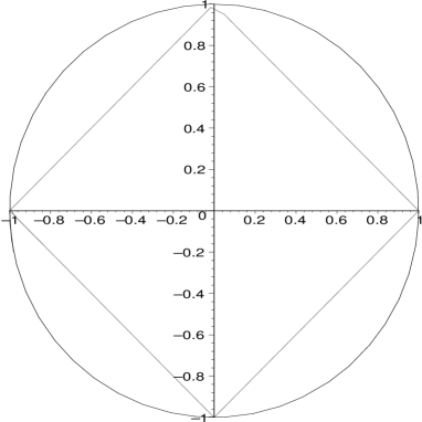
  Figure 8: LTI stability circle and non-linear contraction square in complex plane

  $\Box$

• Example 9.3

  : Consider the 2D lighthouse problem in figure 4 of navigating a vehicle using only azimuth measurements $y^{i}$ to a fixed point in space. The dynamic equations of the vehicle’s motion are

  $${\bf x}^{i+1}={\bf x}^{i}+{\bf u}^{i}$$

  with 2D position ${\bf x}^{i}=(x_{1}^{i},x_{2}^{i})^{T}$ and control input ${\bf u}^{i}=(u_{1}^{i},u_{2}^{i})^{T}$. The vehicle measures only the azimuth to the lighthouse, $\ y^{i}\ =\ \tan\psi^{i}\ =\ \frac{x_{1}^{i}}{x_{2}^{i}}\$.

  

  Figure 9: Lighthouse navigation

  Consider now the observer

  $$\hat{\bf x}^{i+1}=\hat{\bf x}^{i}+{\bf u}^{i}+(\gamma^{i}-1)\left(\begin{array}[]{c}\cos\psi^{i}\\ -\sin\psi^{i}\end{array}\right)\left(\begin{array}[]{cc}\cos\psi^{i}&-\sin\psi^{i}\end{array}\right)\hat{\bf x}^{i}$$ (46)

  From Theorem 8, this observer is semi-contracting for $-1\leq\gamma^{i}\leq 1$. Since the true dynamics is a particular solution of the observer dynamics we can then conclude on global convergence of $\hat{\bf x}^{i}$ to ${\bf x}$.

  In the case of no model or measurement uncertainty, the optimal choice of $\gamma^{i}$ is 0. Otherwise, the choice of $\gamma^{i}$ should trade-off the effect of these uncertainties, as e.g. in the contraction-based strap-down observer of [39].

  Let us now compute the Jacobian of (46)

  $$\frac{\partial{\bf f}^{i}}{\partial{\bf x}^{i}}=\left(\begin{array}[]{cc}\cos\psi^{i}&\sin\psi^{i}\\ -\sin\psi^{i}&\cos\psi^{i}\end{array}\right)\left(\begin{array}[]{cc}\gamma^{i}&0\\ 0&1\end{array}\right)\left(\begin{array}[]{cc}\cos\psi^{i}&-\sin\psi^{i}\\ \sin\psi^{i}&\cos\psi^{i}\\ \end{array}\right)$$

  We can compute for constant $\gamma^{i}=\gamma$ e.g. with MAPLE the square of the largest singular value of $\frac{\partial{\bf f}^{i+1}}{\partial{\bf x}^{i+1}}\frac{\partial{\bf f}^{i}}{\partial{\bf x}^{i}}$ as

  $$\frac{1}{2}(\gamma^{4}+1)\cos(\psi^{i+1}-\psi^{i})^{2}+\gamma^{2}\sin(\psi^{i+1}-\psi^{i})^{2}$$

  $$+\frac{1}{2}|\cos(\psi^{i+1}-\psi^{i})(\gamma^{2}-1)||\cos(\psi^{i+1}-\psi^{i})^{2}(\gamma^{2}-1)^{2}+4\gamma^{2})|^{-\frac{1}{2}}$$ (47)

  which simplifies for $\gamma=0$ to $|\cos(\psi^{i+1}-\psi^{i})|^{2}$. Using equation (42) in Theorem 8 for $\sigma_{1}^{i}=\sigma_{2}^{i}=0$ the exponential contraction rate is for $\gamma=0$

  $$\eta^{i+1}\eta^{i}\geq|\cos(\psi^{i+1}-\psi^{i})|$$ (48)

  Thus, we can conclude on contraction behaviour over several measurement updates if $\psi^{i}$ changes over different $i$.

  Let us now illustrate the above results with simple simulations in the 2D case with position $x_{1}^{i}$ and $x_{2}^{i}$ over the time index $i$ with measurement $y^{i}$.

  Figure 10 shows the motion of a vehicle with constant velocity vector, which is initially tangential to the lighthouse. Due to the tangential motion leads the observer (46) with $\gamma=0$ to global exponential convergence to the real trajectory with convergence rate (48).

  

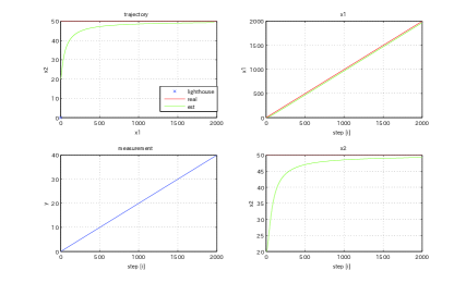
  Figure 10: Tangential movement with respect to lighthouse

  Figure 11 shows a vehicle with constant velocity vector radial to the lighthouse. The observer (46) with $\gamma=1$ achieves global semi-contraction behaviour, i.e. the tangential error disappears, whereas the non-observable radial error remains.

  

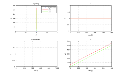
  Figure 11: Radial movement with respect to lighthouse

  Consider now the 3D lighthouse problem of navigating a vehicle using only azimuth $\psi^{i}$ and elevation measurements $\theta^{i}$ to a fixed point in space. The position dynamics of the vehicle’s motion is

  $${\bf x}^{i+1} = {\bf x}^{i}+{\bf u}^{i}$$

  with 3D position ${\bf x}^{i}=(x_{1}^{i},x_{2}^{i},x_{3}^{i})^{T}$ and control input ${\bf u}^{i}=(u_{1}^{i},u_{2}^{i},u_{3}^{i})^{T}$. The vehicle measures only azimuth $\ y_{1}^{i}\ =\ \tan\psi^{i}\ =\ \frac{x_{1}^{i}}{x_{2}^{i}}\$ and elevation $\ y_{2}^{i}\ =\ \tan\theta^{i}=\frac{x_{3}^{i}}{\sqrt{x_{1}^{i}x_{1}^{i}+x_{2}^{i}x_{2}^{i}}}\$ to the lighthouse.

  The measurement equations can be rewritten in a LTV form in ${\bf x}^{i}$ as

  $$x_{2}^{i}\tan\psi^{i}-x_{1}^{i} = 0$$

  $$x_{2}^{i}\tan\xi^{i}-x_{3}^{i} = 0$$

  $$x_{1}^{i}\tan\zeta^{i}-x_{3}^{i} = 0$$

  with $\tan\xi^{i}=\frac{\tan\theta^{i}}{\cos\psi^{i}}$ and $\tan\zeta^{i}=\frac{\tan\psi^{i}\tan\theta^{i}}{\cos\psi^{i}}$.

  Consider now the observer

  $$\hat{\bf x}^{i+1}=\hat{\bf x}^{i}+{\bf u}^{i} + (a^{i}(i)-1)\left(\begin{array}[]{c}\cos\psi^{i}\\ -\sin\psi^{i}\\ 0\end{array}\right)\left(\begin{array}[]{ccc}\cos\psi^{i}&-sin\psi^{i}&0\end{array}\right)\hat{\bf x}^{i}$$ (53)

  $$+ (b^{i}(i)-1)\left(\begin{array}[]{c}0\\ -\sin\xi^{i}\\ \cos\xi^{i}\end{array}\right)\left(\begin{array}[]{ccc}0&-\sin\xi^{i}&\cos\xi^{i}\end{array}\right)\hat{\bf x}^{i}$$ (58)

  $$+ (c^{i}(i)-1)\left(\begin{array}[]{c}-\sin\zeta^{i}\\ 0\\ \cos\zeta^{i}\end{array}\right)\left(\begin{array}[]{ccc}-\sin\zeta^{i}&0&\cos\zeta^{i}\end{array}\right)\hat{\bf x}^{i}$$ (63)

  This dynamics is a superposition of the 2D-lighthouse problem. Hence we can conclude horizontally with (47) or (48) on exponential convergence over several measurement updates if $\psi^{i}$ changes over different $i$. The vertical exponential convergence rate is then given by the minimum of $|b^{i}|$ or $|c^{i}|$.

  Since the true dynamics is a particular solution of the observer dynamics we can then conclude on global exponential convergence of $\hat{\bf x}^{i}$ to ${\bf x}$. $\Box$

10 Concluding Remarks

This paper derives, for non-linear time-varying systems in controllability form

$${\bf x}^{(n)} = {\bf f}({\bf x},...{\bf x}^{(n-1)},t)$$

$${\bf x}^{i+n} = {\bf f}({\bf x}^{i},...{\bf x}^{i+n-1},i)$$

simple controller designs in Theorem 3 and 6 to achieve specified exponential state-and time-dependent convergence rates. The approach can also be regarded as a general gain-scheduling technique with global exponential stability guarantees. The resulting design is illustrated for real and complex time- and state-dependent contraction rates, inclusive the inverted pendulum.

A dual observer design technique is also derived for non-linear time-varying systems in observability form

$${\bf x}^{(n)} = {\bf a}_{1}^{(n-1)}({\bf x},t)+{\bf a}_{2}^{(n-2)}({\bf x},t)+...+{\bf a}_{n}({\bf x},t)$$

$${\bf x}^{i+n} = {\bf a}_{1}^{(+n-1)}({\bf x}^{i},i)+{\bf a}_{2}^{(+n-2)}({\bf x}^{i},i)+...+{\bf a}_{n}({\bf x}^{i},i)$$

, where so far straightforward observer techniques were not known. The resulting observer design is illustrated for non-linear chemical plants, the Van-der-Pol oscillator, the discrete logarithmic map series prediction and lighthouse navigation problem.

These results allow one to shape state- and time-dependent global exponential convergence rates ${\bf\Lambda}_{j}({\bf z}_{j},t)$ and ${\bf\Sigma}_{j}({\bf z}_{j},t)$ ideally suited to the non-linear or time-varying system with the generalized characteristic equation

$$\left(\frac{d}{dt}-\int{\bf\Lambda}_{p}d\right)\Re...\left(\frac{d}{dt}-\int{\bf\Lambda}_{1}d\right){\bf x} = {\bf 0}$$

$$\left({}^{(+1)}-\int{\bf\Sigma}_{p}d\right)\Re...\left({}^{(+1)}-\int{\bf\Sigma}_{1}d\right){\bf x}^{i} = {\bf 0}$$

with $\Re({\bf z}_{1})={\bf x},\Re({\bf z}_{j+1})=\dot{\bf z}_{j}-\int{\bf\Lambda}_{j}({\bf z}_{j},t)d{\bf z}_{j}$ ( $\Re({\bf z}_{1}^{i})={\bf x}^{i},\Re({\bf z}_{j+1}^{i})={\bf z}_{j}^{i+1}-\int{\bf\Sigma}_{j}({\bf z}_{j}^{i},i)d{\bf z}_{j}^{i}$ ).

Analytic exponential robustness bounds on general non-linear, time-varying distortions ${\bf d}$ on the right-hand side of the characteristic equation are given with $\eta$ in Theorem 5 or 8. Both theorems can also be used to derive analytic state- and time-dependent approximated convergence rates for given general non-linear, time-varying higher-order systems.

Note that the general technique of this paper matches the eigenvalue analysis for LTI systems. For non-LTI systems additional time derivatives for continuous systems and index changes for discrete systems of the contraction rates have to be considered. Only with these changes exponential convergence guarantees with the time- and state-dependent contraction rates are given.

References

[1] Aghannan, N., Rouchon, P., An Intrinsic Observer for
a Class of Lagrangian Systems, IEEE Transactions on Automatic
Control, 48(6), 2003.
[2] Angeli, D., A Lyapunov approach to incremental
stability properties, IEEE Transactions on Automatic Control,
47, 2002.
[4] Aylward E., Parrilo P., and J.J.E. Slotine,
Stability and Robustness Analysis of Non-Linear Systems via
Contraction Metrics and SOS Programming, Automatica, 44(8), 2008
[5] Bekris, Evaluation of Algorithms for Bearings-Only
SLAM, e, IEEE International Conference on Robotics and
Automation, Orlando, FL, 2006.
[6] Bertsekas, D., and Tsitsiklis, J., Parallel and
distributed computation: numerical methods, Prentice-Hall, 1989.
[7] Bryson A., Ho, Y., Applied Optimal Control, Taylor and Francis, 1975.
[8] Chung Soon-Jo, Slotine, J.J.E, Cooperative Robot
Control and Concurrent Synchronization of Lagrangian Systems, IEEE Transactions on Robotics, Vol. 25, No. 3, June 2009.
[9] Fliess M., Levine J., Martin Ph., and Rouchon P.,
Flatness and defect of non-linear systems: introductory theory and
examples. International Journal of Control, 61(6), 1995.
[10] Hartmann, P. Ordinary differential equations, John
Wiley Sons, New York, 1964.
[11] Isidori, A., Non-Linear Control Systems, 3rd Ed.,
Springer Verlag, 1995.
[12] Kailath, T., Linear Systems, Prentice Hall,
1980.
[13] Krasovskii, N.N., Problems of the Theory of Stability
of Motion, Mir, Moskow, 1959.
[14] Lawrence, D.A., and Rugh, W.J., Gain-scheduling
dynamic linear controllers for a non-linear plant, Automatica,
31(3), 1995.
[15] Lee, H.G., Arapostathis, A., Marcus, S.I., Linearization
of discrete-time systems, International Journal of Control,
volume 45, number 5, 1987.
[16] Lewis, D.C., Metric properties of differential
equations, American Journal of Mathematics, 71, 1949.
[17] Lohmiller, W., and Slotine, J.J.E., On Metric
Controllers for Non-Linear Systems, IEEE Conference on Decisioin
and Control, Kobe, Japan, 1996.
[18] Lohmiller, W., and Slotine, J.J.E., On Contraction
Analysis for Non-Linear Systems, Automatica, 34(6), 1998.
[19] Lohmiller, W., and Slotine, J.J.E., Non-Linear Process
Control Using Contraction Theory, A. I. Che. Journal, March
2000.
[20] Lohmiller, W., and Slotine, J.J.E., Control System
Design for Mechanical Systems Using Contraction Theory, IEEE
Transactions on Automatic Control, 2000.
[21] Lohmiller, W., and Slotine, J.J.E., Contraction
Analysis of Non-Linear Distributed Systems, International Journal
Of Control, 78(9), 2005.
[22] Lohmiller, W, Contraction Analysis of Nonlinear
Systems, PhD Thesis at M.I.T., 1998.
[23] Lohmiller, W., and Slotine, J.J.E., Shaping
state-dependent convergence rates in non-linear control system design,
AIAA Guidance, Navigation, and Control Conference, 2008.
[24] Lohmiller, W., and Slotine, J.J.E., Exact Modal
Decomposition of Nonlinear Hamiltonian Systems,
AIAA Guidance, Navigation, and Control Conference, 2009.
[25] Lovelock D., and Rund, H., Tensors, Differential
Forms, and Variational Principles, Dover, 1989.
[26] Mracek, P., Cloutier, J., D’Souza C., A new Technique
for Non-Linear Estimation, I.E.E.E. International Conference on
Control Applications, Dearborn, Michigan, 1996.
[27] Nguyen, T.D., and Egeland, O. Observer Design for a
Towed Seismic Cable, American Control Conference, Boston, 2004
[28] Moritz N., and Osterhuber R. Three-Stage
Gradient-Based Optimization Scheme in Design of Feedback Gains within
Eurofighter Primary Control Laws, AIAA Guidance, Navigation, and
Control Conference, 2006.
[29] Nijmeijer, H., and Van der Schaft, A., Non-Linear
Dynamical Control Systems, Springer Verlag, 1990.
[30]Opial, Z., Sur la stabilité asymptotique des
solutions d’un système d’équations différentielles, Ann. Polinici Math, 7, 1960.
[31] Reboulet, C., and Champetier, C., A new method for
linearizing non-linear systems: the pseudo-linearization, International Journal of Control, 40, page 631, 1984.
[32] Schmalz, C., Lohmiller W. and Koehler T.,
Analytic error computation of the Strap-Down-Algorithm, AIAA
Conference, 2007.
[33] Seifert, G., On stability in the large for periodic
solution of differential systems, Annals of Math, 67(1), 1958.
[34] Shamma, J., and Gurdal, A., Dynamic Fictitious Play,
Dynamic Gradient Play and Distributed Convergence to Nash Equilibra,
IEEE Transactions on Automatic Control, March 2005.
[35] Slotine and Li, Applied Non-Linear Control, Prentice Hall, 1991.
[36] Slotine, J.J.E., and Lohmiller, W. Modularity,
Evolution, and the Binding Problem: A View from Stability Theory, Neural Networks, 14(2), 2001.
[37] Wang, W., and Slotine, J.J.E., On Partial Contraction
Analysis for Coupled Nonlinear Oscillators, Biological
Cybernetics, 92(1), 2004.
[38] Zeitz, M., The extended Luenberger observer for
non-linear systems, Systems and Control Letters 9 (1987) 149-156,
1987.
[39] Zhao, Y., and Slotine, J.J.E., Discrete Non-Linear
Observers for Inertial Navigation, Systems and Control Letters,
54(8), 2005.