The ACS Fornax Cluster Survey. VIII. The Luminosity Function of Globular Clusters in Virgo and Fornax Early-Type Galaxies and its Use as a Distance Indicator

Abstract

We use a highly homogeneous set of data from 132 early-type galaxies in the Virgo and Fornax clusters in order to study the properties of the globular cluster luminosity function (GCLF). The globular cluster system of each galaxy was studied using a maximum likelihood approach to model the intrinsic GCLF after accounting for contamination and completeness effects. The results presented here update our Virgo measurements and confirm our previous results showing a tight correlation between the dispersion of the GCLF and the absolute magnitude of the parent galaxy. Regarding the use of the GCLF as a standard candle, we have found that the relative distance modulus between the Virgo and Fornax clusters is systematically lower than the one derived by other distance estimators, and in particular it is 0.22mag lower than the value derived from surface brightness fluctuation measurements performed on the same data. From numerical simulations aimed at reproducing the observed dispersion of the value of the turnover magnitude in each galaxy cluster we estimate an intrinsic dispersion on this parameter of 0.21mag and 0.15mag for Virgo and Fornax respectively. All in all, our study shows that the GCLF properties vary systematically with galaxy mass showing no evidence for a dichotomy between giant and dwarf early-type galaxies. These properties may be influenced by the cluster environment as suggested by cosmological simulations.

1. Introduction

The distribution of globular cluster (GC) magnitudes has the remarkable property that it is observed to peak at a value of $M_{V}\approx-7.5$ mag in a near universal fashion (e.g., Jacoby et al. 1992, Harris 2001, Brodie & Strader 2006). This distribution, usually referred to as the GC luminosity function (GCLF), has been historically described by a Gaussian. By virtue of its near universality, the derived mean or “turnover” magnitude $\mu$ has seen widespread use as a distance indicator (e.g. Secker 1992, Sandage & Tammann 1995), even though some dispersion and discrepant results have been reported in the literature (see discussion in Ferrarese et al. 2000a).

There is nevertheless no solid theoretical explanation for the observed universality of the turnover magnitude. The luminosity function is a reflection of the more fundamental mass spectrum of the GCs, and as such the “universal” turnover magnitude corresponds to a cluster mass of $\sim 2\times 10^{5}\mathcal{M_{\odot}}$. Vast efforts have been undertaken from the theoretical point of view in order to explain the underlying universal mass function. The many publications on this topic can be separated into those trying to identify some particular initial condition that selects a certain mass scale for star formation (e.g., Peebles & Dicke 1968, Fall & Rees 1985, West 1993), and those looking for a destruction mechanism that selects clusters in a particular mass range starting from an initially wide mass spectrum (e.g., Fall & Rees 1977, Gnedin & Ostriker 1997, Prieto & Gnedin 2008)

At the high-mass end (i.e. $m_{gc}<\mu$) the mass function of globular clusters resembles very closely the mass function of young clusters and molecular clouds in the Milky Way and other nearby galaxies (see e.g. Harris & Pudritz 1994, Elmegreen & Efremov 1997, Gieles et al. 2006). On the other hand, neither young clusters nor molecular clouds show a turnover on their mass distributions, but they keep rising monotonically following a power-law to lower masses. Fall & Zhang (2001) used simple analytical models (including evaporation by two-body relaxation, gravitational shocks and mass loss by stellar evolution) to study the evolution of the GC mass function. They showed that, for a wide variety of initial conditions, an initial power-law mass function develops a turnover that, after 12 Gyr, is remarkably close to the observed turnover of the GCLF. Vesperini (2000, 2001) reaches a similar conclusion, but finds that a log-normal mass function provides a better fit to the data. Fainter than the turnover, the evolution would be dominated by two-body relaxation, and the mass function would end up having a constant number of GCs per unit mass, reflecting the fact that the masses of tidally limited clusters are assumed to decrease linearly with time until they are destroyed (other authors propose different mass-loss rates, see e.g., Lamers et al. 2006). Brighter than the turnover, the evolution is dominated by stellar evolution at early times and by gravitational shocks at late times. Recently, McLaughlin & Fall (2008) have shown that the GC mass function in the Milky Way depends on cluster half-mass density (i.e. the mean density within a radius containing half the total mass of the GC), in the sense that the turnover mass increases with half-mass density, while the width of the GC mass function decreases. But while there is currently a fairly good understanding of the dynamical processes that shape the GCLF, many details are still missing. In particular none of the theories proposed has been entirely successful on addressing the question of how the turnover magnitude can remain constant regardless of environmental properties and the mass of the host galaxy.

The use of deep HST data during the last years has resulted in high quality GCLF data, reaching 2 magnitudes beyond the turnover at the distance of the Virgo cluster ($\sim$16.5 Mpc, Mei et al. 2007). The use of these deeper observations has recently uncovered a strong correlation between the GCLF dispersion and the absolute magnitude of the parent galaxy (Jordán et al. 2006, 2007b), demonstrating the non-universality of this parameter and, as a consequence, of the GCLF as a whole. Here we present a study of the GCLF of 132 early type galaxies aimed to perform a precise test of the GCLF as a distance indicator by comparing the relative distance between the Virgo and Fornax clusters derived using the GCLF to the one derived using an analysis of surface brightness fluctuations (SBF, Tonry & Schneider 1988) based on the same data (Blakeslee et al. 2009). Previous papers in the this series have presented an introduction to the survey (Jordán et al. 2007a), the properties of the central surface brightness profiles of early-type galaxies (Côté et al. 2007) and a catalog of SBF distances and a precise measurement of the Virgo-Fornax distance (Blakeslee et al. 2009).

The organization of this paper is as follows. In §2 we present a description of the observations and data reduction procedures. In §3 we describe the GCLF model fitting, and in §4 we compare the properties of the fits to previous results regarding the dispersion of the GCLF. Section §5 is focused on determining how universal the value of the turnover magnitude is, while in §6 we look for a better understanding of the external parameters that might affect this value. Finally, in §7 we summarize our results and the main conclusions of this paper.

2. Data and GCLF ingredients

Each one of the 132 galaxies included in this study was observed with the Advanced Camera for Surveys (ACS) during a single Hubble Space Telescope (HST) orbit, as part of the ACS Virgo Cluster Survey (ACSVCS) and the ACS Fornax Cluster Survey (ACSFCS). The goals and main observational features of these two surveys are extensively discussed in Côté et al. (2004) and Jordán et al. (2007a), respectively. We refer the interested reader to these publications for further details.

The surveys targeted a total of 100 galaxies in the Virgo cluster and 43 galaxies in Fornax, and included observations in the F475W ($\approx$ Sloan $g$) and F850LP ($\approx$ Sloan $z$) passbands, with exposure times of $\sim$750s and $\sim$1210s respectively. In what follows we will refer to the F475W filter as “$g$” and to F850LP as “$z$”, due to their close proximity to the corresponding Sloan passbands.

Jordán et al. (2004) describes the pipeline implemented to automate the reduction procedure and analysis of all images in both surveys. The final output from this pipeline is a preliminary catalog of GC candidates and expected contamination per galaxy, including photometric and morphological properties, that are later used to evaluate the probability $p_{GC}$ that a given object is a GC (see Jordán et al. 2009 for details). For the purposes of this study, and as defined on previous ACSVCS and ACSFCS papers, we constructed the GC candidate samples by selecting all sources that have $p_{GC}\geq$0.5.

Our catalog of GC candidates in a given galaxy differs from the intrinsic GC population due to two effects: the existence of contamination in the sample and the level of completeness of the observations.

In order to quantify the average number of contaminants per field of view we have used archival ACS imaging of 17 blank-high latitude fields that have been observed in both the $g$ and $z$ bands, to the same or deeper depth than our images. These control fields were processed using the same pipeline implemented for the science data, and were then used to build customized control fields, as if a given galaxy was in front of it (the details of this process are explained in Peng et al. 2006, were also a full list of the control fields used is available). For each of our target galaxies, the result is a catalog containing 17 different estimates of the expected foreground and background contamination. These are later used to obtain an average estimate of the contamination in the field of view of a given galaxy.

The completeness function needs to be built considering four parameters: the magnitude of the source ($m$), its size as measured by the projected half light radius ($r_{h}$), its color ($(g-z)_{0}$), and the surface brightness of the local background over which the object lies ($I_{b}$). The completeness function $f(m,r_{h},(g-z)_{0},I_{b})$ was obtained by performing simulations that added model GCs of different sizes ($r_{h}=(1,3,6,10)$ pc), colors ($(g-z)_{0}=(0.7,1.1,1.5,1.9)$ mag), and with King (1966) concentration parameter of $c=1.5$ to the images. Although the effect of the color of the clusters has not been considered in previous publications (e.g. Peng et al. 2006, Jordán et al. 2007b), we have now established that it also has a small but measurable effect over the expected completeness. Overall, roughly 6 million fake GCs were added for the completeness tests for each color, with equal fractions at each of the four sizes and avoiding physical overlaps with sources already present. These images were then reduced through exactly the same procedure used with the science data. The final output of the process is a four dimensional table that is used to evaluate $f$ given an arbitrary set of $(m,r_{h},(g-z)_{0},I_{b})$. The random uncertainty in the mean completeness curve is essentially zero, so the completeness limits at 90% and 50% are robust and can be determined with negligible error for a given population of objects.

This paper focuses on the study of the 89 early-type galaxies discussed by Jordán et al.(2007b) and all 43 galaxies of the ACSFCS. Our analysis is restricted to those galaxies that have more than five GC candidates and for which we were able to usefully constrain the GCLF parameters. These restrictions exclude 11 galaxies in the Virgo sample but none in Fornax.

3. GCLF Model Fitting

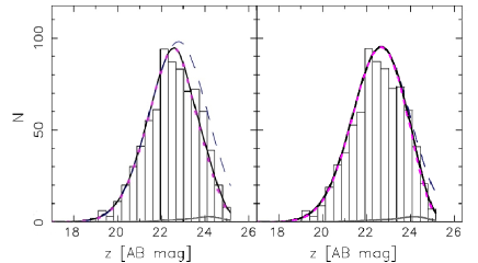
Figure 1.— Left: GCLF histogram for VCC1226 as presented in Jordán et al. (2007b). The lines show the best-fit model (solid black curve), the intrinsic Gaussian component (dashed curve), the Gaussian component multiplied by the expected completeness (dotted curve), and a kernel density estimate of the expected contamination (solid gray curve). Right: The same as shown in the left hand side, but now using the corrected completeness function.

Given the observational information previously described we aim to recover the parameters of the intrinsic luminosity function of the GCs in a galaxy. We used a maximum likelihood approach similar to the one described by Secker & Harris (1993). According to this formalism, and as detailed in Jordán et al. (2007b), we describe the intrinsic GCLF by some function $G(m\!\mid\!\Theta)$, with $\Theta$ being the set of model parameters to be fitted, and we assume that the uncertainties on magnitude measurements $\epsilon_{m}$ have a Gaussian distribution. In absence of contamination, the probability of observing a GC with a given effective radius $R_{h}$ and apparent magnitude $m$ against a galaxy background $I_{b}$ would be:

$$\small G_{T}(m\!\mid\!\Theta,R_{h},I_{b},\epsilon_{m})=\mathcal{A}[\ h(m\!\mid\!\epsilon_{m})\,\otimes\,G(m\!\mid\!\Theta)\ ]f(m,R_{h},I_{b}),$$ (1)

where $h(m\!\mid\!\epsilon_{m})=(2\pi\epsilon^{2}_{m})^{-1/2}\mathrm{exp}(-m^{2}/2\epsilon^{2}_{m})$, is the magnitude error distribution, which is convolved with the intrinsic GCLF $G(m\!\mid\!\Theta)$. The normalization factor $\cal A$ is a function of the GCLF parameters $\Theta$ and the GC properties $R_{h}$, $I_{b}$, and $\epsilon_{m}$, and it is set by requiring that $G_{T}$ integrates to unity over the whole magnitude range covered by the observations.

In practice a fraction $\mathcal{B}$ of the sources classified as GC candidates in a galaxy are contaminants, so that the probability of observing a  GC  with parameters $(m,R_{h},I_{b},\epsilon_{m})$ is reduced by a factor $(1-\mathcal{B})$ and the distribution that accounts for all the observed objects has to include the contaminants luminosity function $b(m)$. Thus, the likelihood of observing a total number of N objects with magnitudes $m_{i}$ and properties $(R_{h},I_{b},\epsilon_{m})$ is

$$\mathcal{L}(\Theta,\mathcal{B})=\prod^{N}_{i=1}[(1-\mathcal{B})G_{T}(m_{i}\!\mid\!\Theta,R_{h,i},I_{b,i},\epsilon_{m,i})+\mathcal{B}b(m_{i})],$$ (2)

Jordán et al. (2007b) have made a detailed description of several parametrization of the GCLF and their various advantages and drawbacks. Here we focus on the study of the Gaussian representation, because of its historic use in the study of the GCLF as a distance indicator. It is worth noticing that other parametrization such a $t_{5}$ function have also been successfully used for this purpose (Secker 1992, Kissler et al. 1994). For the case of a Gaussian the set of model parameters will be $\Theta\equiv\{\mu,\sigma_{m}\}$, where $\mu$ and $\sigma$ are the turnover and the dispersion in a distribution of the form:

$$\frac{dN}{dm}=\frac{1}{\sqrt{2\pi}\sigma}\ \mathrm{exp}\left[-\frac{(m-\mu)^{2}}{2\sigma^{2}}\right]$$ (3)

Figure 2.— Difference in turnover magnitude produced by using the completeness function presented by Jordán et al. 2007b and the one we are using here ($\Delta\mu\equiv\mu_{old}-\mu_{new}$) in the $g$ (top) and $z$ (bottom) bands, vs. the $B$-band apparent magnitude of the parents galaxy.

The coding implementation of the outlined maximum likelihood procedure is in practice the same used to compute the GCLF by Jordán et al. (2007b), except that we are now using completeness curves customized to the Fornax data too. Also, during the analysis of the ACSFCS data we found a coding mistake in the interpolation of the completeness curves previously used to estimate the GCLF parameters of the Virgo galaxies. The background information in the completeness curves was sometimes misread in such a way that the completeness level assigned to a given background brightness was lower than the real value. As the changes in completeness are more significant for brighter backgrounds, massive galaxies were more affected than dwarf galaxies. Even though it does not have any significant effect over the main conclusions of Jordán et al. (2007b), we are reporting the problem here because it produces a slight change in the turnover magnitudes of the Virgo galaxies. The massive galaxies are the most affected, with their turnover magnitudes becoming roughly $\sim$0.1 mag brighter. This behavior can be observed in Figure 1, where we have plotted side-by-side the $z$-band GCLF fit for VCC1226 as presented in Figure 4 of Jordán et al. (2007b), and the current fit implemented using the corrected completeness function that now also includes a color correction. In Figure 2 we have plotted the observed change in the turnover magnitude ($\Delta\mu\equiv\mu_{old}-\mu_{new}$) in both bands, against the $B$-band apparent magnitude of the parent galaxy, showing that the brightest galaxies are the most evidently affected, unlike the dwarfs whose turnover stays virtually unchanged. Some spread can be observed in the case of the intermediate-luminosity galaxies, but in all cases the change in $\mu$ is always lower than 0.15 mag.

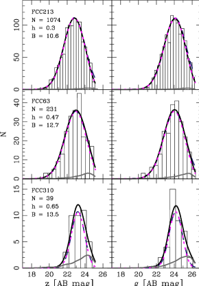
Figure 3.— GCLF histograms for the Virgo and Fornax sample galaxies. For each one of them we present the z- and $g$-band GCLFs side by side. The VCC/FCC name and $B$-band magnitude of the galaxy are indicated in the upper left corner of the left panel, where we also indicate the total number of sources $N$ in each histogram and the bin width $h$ used to construct it ($h$ is calculated as described in the text). In addition, we show the best-fit model (solid black curve), the intrinsic Gaussian component (dashed curve), the Gaussian component multiplied by the expected completeness (dotted curve), and a kernel density estimate of the expected contamination in the sample (solid gray curve). The solid black curve is the sum of the solid gray and dotted curves. The galaxies are ordered by decreasing apparent $B$-band total luminosity, reading down from the upper left corner. The parameters of the fits are given in Table 1 and 2. The full version of this figure is published in the electronic edition of the Astrophysical Journal. Sample panels are shown here for guidance regarding its form and content.

Table 1 lists the corrected values for the Gaussian GCLF parameters of the ACSVCS galaxies. Updated values for the evolved-Schechter function fits presented by Jordán et al. (2007b) will be presented elsewhere. The Gaussian parameters shown in Table  1 are the ones considered for this publication and they should be used for future reference. This table includes, for all the ACSVCS galaxies: the $B$-band apparent magnitude from Binggeli et al. (1985), the estimated GCLF parameters in both bands, the fraction of objects that are considered to be contaminants, and the total number of globular cluster candidates (including contaminants). Table 2 presents the equivalent information computed for the ACSFCS galaxies, including the $B$-band absolute magnitude from Ferguson (1989a). Figure 3 shows the $z$ and $g$-band GCLF histograms of the sample galaxies, ordered by decreasing apparent $B$-band total luminosity. The dashed curve corresponds to the intrinsic Gaussian component given by Equation 3 and the parameters in Table 2. The Gaussian component multiplied by the expected completeness is represented by the dotted curve, and a kernel density estimate of the expected contamination in the sample appears as a solid gray curve. The solid black curve is the sum of the solid gray and dotted curves, and corresponds to the net distribution for which the likelihood in Equation 2 is maximized. The name and apparent B magnitude of the galaxy are indicated in the upper left corner of the left panel, where we also quote the total number of sources in each histogram and the bin width h. The width of the bins, used only for display purposes here, follows the rule $h=2(\textsc{IQR})N^{-1/3}$ , where $(\textsc{IQR)}$ is the interquartile range of the magnitude distribution and $N$ is the total number of objects in each GC sample (Izenman, 1991).

Figure 4.— Left: Estimate of Gaussian dispersion in the $z$ band, $\sigma_{z}$, vs. the same quantity in the $g$ band, $\sigma_{g}$ , for the GCLFs of our Fornax sample. Uncertainties are 1$\sigma$. The line marks the one-to-one correspondence between these two quantities. Right: Difference between estimates of Gaussian means in the $g$ and $z$ bands, $\mu_{g}-\mu_{z}$ , vs. the mean color $\langle g-z\rangle$ of the GC systems of our sample galaxies. Uncertainties are 1$\sigma$. The line marks the one-to-one correspondence between these two quantities.

As a sanity check of our fitting procedure, in the left-hand side of Figure 4 we compare the Gaussian dispersion inferred from the GCLF fit in each band, $\sigma_{g}$ vs. $\sigma_{z}$, including only data from the Fornax sample. In the right-hand side of the same figure we have plotted the difference between estimates of Gaussian means in the $g$ and $z$ bands $(\mu_{g}-\mu_{z})$, vs. the mean color $\langle g-z\rangle$ of the GC systems of our sample galaxies. From the very tight correlation between the measurements in different bands we conclude that the GCLF fitting procedure is internally consistent and also that our error estimations are realistic.

4. The $\sigma-M_{B,gal}$ Relation

One of the main results discussed in Jordán et al. (2006, 2007b) is the existence of a strong correlation between the dispersion of the GCLF $\sigma$, and the $B$-band absolute magnitude of the host galaxy $M_{B,gal}$, with brighter galaxies showing higher dispersion values. Even though some suggestive evidence on this respect was previously presented by other authors (e.g. Kundu & Whitmore, 2001) the high precision and homogeneity of our ACS/HST data unveiled the $\sigma-M_{B,gal}$ correlation as a general trend in GC systems, which was later extended to still higher galaxy luminosity by Harris et al. (2009) using 5 giant elliptical galaxies in the Coma cluster. Figure 5 shows this correlation for all the 132 galaxies in our sample in both bands, now using the homogeneous $z$-band absolute magnitudes derived from the apparent magnitudes estimated by Ferrarese et al. (2006) and Côté et al. (2010, in preparation) and the corresponding distance moduli published by Blakeslee et al. (2009). These values were corrected for reddening assuming $A_{z}=1.485\ E(B-V)$ (Ferrarese et al. 2006) where the value of $E(B-V)$ was taken from Schlegel et al. (1998). In this figure we have used different symbols in order to identify the galaxies according to their morphological classification, but no particular trend related to this property seems to be obvious. The straight lines drawn in the panels correspond to error-weighted linear characterizations of these trends:

$$\sigma_{z}=(1.07\pm 0.02)-(0.10\pm 0.01)(M_{z,gal}+22)$$ (4)

and

$$\sigma_{g}=(1.10\pm 0.01)-(0.10\pm 0.01)(M_{z,gal}+22).\\$$ (5)

We have excluded from these fits three galaxies for which no z-band magnitudes are available: VCC1535, VCC1030, and FCC167. Although shown in Figure 5, FCC21 (=NGC1316) is also not included on the fits because the observed GC system in this galaxy is highly influenced by interaction and proximity with its satellite galaxies, and therefore our GCLF fit is not reliable. Unlike Jordán et al. (2006, 2007b) we have now also excluded from the analysis four galaxies in the Virgo cluster (VCC1297, VCC1199, VCC1192 and VCC1327) and two galaxies in Fornax (FCC202 and FCC143) because their GC systems appear to be contaminated by their proximity to massive ellipticals. All these galaxies are nonetheless retained in the Tables for completeness.

Equations 4 and 5 confirm the trend previously observed in Virgo, and with higher statistical significance, by including the Fornax data. This result shows by itself that the GCLF parameters are not universal and depend at least on one parameter, i.e. the luminosity of the parent galaxy, adding an additional feature that needs to be accounted for by theories aiming to explain the shape of the GCLF.

When the data corresponding to each cluster are fitted independently the linear characterizations obtained are, in the case of Virgo:

$$\sigma_{z}=(1.09\pm 0.01)-(0.08\pm 0.01)(M_{z,gal}+22),$$ (6)

$$\noindent\sigma_{g}=(1.11\pm 0.01)-(0.09\pm 0.01)(M_{z,gal}+22);$$ (7)

and for the Fornax cluster:

$$\sigma_{z}=(1.07\pm 0.04)-(0.13\pm 0.02)(M_{z,gal}+22),$$ (8)

$$\noindent\sigma_{g}=(1.09\pm 0.03)-(0.10\pm 0.01)(M_{z,gal}+22).$$ (9)

This translates into a $0.05-0.1$ mag difference in dispersion at $M_{z}\sim 22$, and also shows that the linear fits derived from both sets of data are equivalent within the uncertainties.

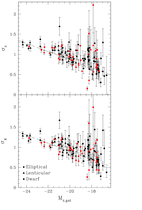
Figure 5.— Top: GCLF dispersion $\sigma_{z}$, inferred from Gaussian fits to the $z$-band data, vs. galaxy $M_{z,gal}$. The dashed line corresponds the linear relation between $\sigma_{z}$ and $M_{z,gal}$ in eq. 4. Bottom: Same comparison, but for the Gaussian dispersion of the $g$-band GCLFs, $\sigma_{g}$. The dashed line represents eq. 5. In both panels the black symbols correspond to Virgo galaxies, and the red ones to the sample in the Fornax cluster. We have morphologically separated the galaxies into elliptical (circles), lenticular (triangles), and dwarf (squares) galaxies.

As discussed in Jordán et al. (2006) it is rather straightforward to link this trend in luminosity dispersion with a similar trend in the mass distribution of GCs. It is well known that giant galaxies tend on average to have more metal-rich GC populations when compared to dwarfs, showing also larger dispersions in metallicity (see e.g. Peng et al. 2006). This result, added to the dependence of the cluster mass-to-light ratios ($\Upsilon$) on metallicity, opens the possibility that the observed dispersion in the value of $\sigma$ might be metallicity-driven. These variations in $\Upsilon$ have a strong dependence on wavelength. In bluer filters (the $g$-band in our case), variations of a factor of 2 or more in $\Upsilon$ can be observed in the typical metallicity range of GCs ($-2\leq$ [Fe/H] $\leq 0$). At redder wavelengths this variation becomes less dramatic, as shown by old stellar population models (e.g. PEGASE population synthesis models; Fioc & Rocca-Volmerange, 1997). In particular the expected variation in $\sigma$ as a consequence of changes of $\Upsilon$ in our $z$-band measurements should not be higher than $\sim$ 4%, which means that the spread in the value of $\sigma$ observed in the upper panel of Figure 5 reflects almost entirely a trend in the mass distribution of globular clusters. Moreover, the very similar values obtained for $\sigma$ in the $z$- and $g$-bands shows immediately that the trend of $\sigma$ with $M_{B}$ cannot be generated by metallicity-driven changes in $\Upsilon$.

5. A Relative Virgo-Fornax Distance Estimation

Several methods have been used in order to obtain accurate distance estimations for both the Virgo and Fornax clusters, a task that is in general more easily achieved in the case of Fornax due to its more compact nature. The Virgo cluster extends for over 100 deg² in the sky, showing a complex and irregular structure, with galaxies of different morphological type showing different spatial and kinematic distributions. Working on these conditions the various distance estimators have reached different levels of accuracy (see Ferrarese et al. 2000a, 2000b). We will discuss now a compilation of results from the literature, which are also summarized in Table 3.

The HST Key Project to measure the Hubble constant aimed at obtaining accurate distances to galaxies using the period-luminosity relation for Cepheid variables (their final results are presented in Freedman et al. 2001). It included the identification of Cepheids belonging to 6 spiral galaxies in Virgo and 2 in Fornax, that were used to estimate the distance to their parent galaxies, and then to the corresponding clusters. This resulted in distance moduli of $(m-M)_{V}=30.92\pm 0.05$ mag and $(m-M)_{F}=31.39\pm 0.20$ mag for Virgo and Fornax respectively, which translates into a relative distance modulus of $\Delta(m-M)=0.47\pm 0.20$ mag.

D’Onofrio et al. (1997) derived the relative distance between Virgo and Fornax by applying the D${}_{n}-\sigma$ (Dressler et al., 1987) and the fundamental plane (Djorgovski & Davis, 1987) relations to a homogeneous sample of early-type galaxies. The two distance indicators gave consistent results with a relative distance modulus of $\Delta(m-M)=0.45\pm 0.15$ mag. These results are in close agreement with the value $\Delta(m-M)=0.52\pm 0.17$ mag later published by Kelson et al. (2000) obtained also by using the fundamental plane and D${}_{n}-\sigma$ relations built from data calibrated by the aforementioned Cepheid distances to spiral galaxies in both Virgo and Fornax.

The planetary nebula luminosity function (PNLF) has also been used for measuring distances in the local Universe. Ciardullo et al. (1998) determined a distance modulus of $(m-M)_{V}=30.79\pm 0.16$ mag to M87, in good agreement with previous measurements (e.g. Jacoby et al., 1990). McMillan et al. (1993) used the PNLF to determine the distance to three galaxies in Fornax, obtaining a mean distance to the cluster of $(m-M)_{F}=31.14\pm 0.14$ mag. If we consider M87 to be at the center of Virgo, the corresponding relative distance modulus would be $\Delta(m-M)=0.35\pm 0.21$ mag. Ferrarese et al. (2000a) calibrated literature measurements of the PNLF using Cepheids, which led them to estimate a relative distance modulus between Virgo and Fornax of $\Delta(m-M)=0.30\pm 0.10$ mag when considering the A-subcluster as indicative of the distance to Virgo.

Earlier relative distance modulus results derived by using the GCLF as distance indicator present some hints of disagreement with the other estimations discussed here. Even though they were working with small and rather heterogeneous samples, previous studies tend to put this value around a very low $\Delta(m-M)\sim 0.13$ mag (e.g. Kohle et al. 1996, Blakeslee & Tonry 1996, Ferrarese et al. 2000a, Richtler 2003).

One of the most reliable distance estimators when it comes to population II samples is the surface brightness fluctuations (SBF) method due to its high internal precision. The ACS Virgo and Fornax clusters surveys, among whose aims is studying GC properties and measuring surface brightness fluctuations, provide us with the ideal data for comparing the properties of the GCLF as a distance estimator with SBF results. We will discuss these results separately in the next session.

5.1. SBF distances

The method of SBF was first introduced by Tonry & Schneider (1988), and uses the fluctuations produced in each pixel of an image by the Poissonian distribution of unresolved stars in a galaxy in order to estimate the distance to the object. The amplitude of those surface brightness fluctuations normalized to the underlying mean galaxy luminosity are inversely proportional to distance and can therefore be used as a distance indicator (see Blakeslee et al. 1999 for a review).

The distances to the Virgo galaxies included in the ACSVCS have been measured using the SBF method. Mei et al. (2005a) describes the reduction procedure used for the surface brightness analysis of the ACSVCS data, and Mei et al. (2005b) presents the calibration for giant and dwarf early-type galaxies. Finally, Mei et al. (2007) introduces the distance catalog for a total 84 galaxies (50 giants and 34 dwarf) for which the SBF method was successfully implemented, delivering at the same time a three dimensional map of the structure of the Virgo cluster. These distance values were later updated and the measurements extended to include the 43 early-type galaxies of the ACSFCS in Blakeslee et al. (2009). In our analysis we will use the consistent set of Virgo and Fornax distances presented by the later publication. When no SBF distance is available for one of our sample galaxies, we assume it is located at the mean Virgo distance ($(m-M)=31.09$ mag) adopted by Mei et al. (2007). This estimate is based on ground-based I-band SBF measurements calibrated against Cepheids distances (Tonry et al. 2000, Freedman et al. 2001).

From their SBF measurements Blakeslee et al. (2009) derives a relative Virgo-Fornax distance modulus of $\Delta(m-M)=(0.42\pm 0.03)$ mag, which locates the Fornax cluster at a distance of $d_{F}=20$ Mpc ($(m-M)_{F}=31.5$ mag). This value is in good agreement with the relative distance moduli derived from the other distance estimators discussed above and summarized in Table 3, but it is significantly more precise.

5.2. $\mu_{z}$ as Distance Indicator

One of the main problems in understanding the properties of the turnover of the GCLF as distance indicator is the lack of homogeneity in the data. The most comprehensive compilation of recent data (mainly HST observations) was presented by Richtler (2003), including a total of 102 turnover magnitudes coming from at least 8 different publications. This inhomogeneity introduces a major source of uncertainty in the analysis, as one has to rely on each author’s results irrespective of the fact that they might not be using the same procedure to reduce the data, the observations might not be on the same photometric band, and they might not even be using the same analytic form to fit the GCLF.

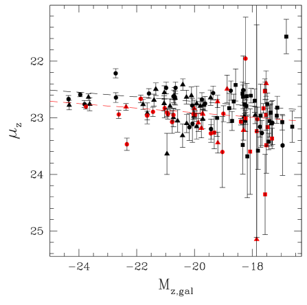
Figure 6.— GCLF turnover magnitude, $\mu_{z}$, inferred from Gaussian fits to the $z$-band data, vs. $z$-band galaxy absolute magnitude $M_{z,gal}$, for all the galaxies in the ACS Virgo (black symbols) and Fornax (red symbols) cluster surveys. The lines represent a simultaneous error-weighted linear fit performed over both samples, that corresponds to $\mu_{z}=(23.51\pm 0.11)+(0.04\pm 0.01)M_{z,gal}$, plus and offset of $\Delta(m-M)=0.20\pm 0.04$ mag for the galaxies in Fornax. The sample has been morphologically separated into elliptical (circles), lenticular (triangles), and dwarf (squares) galaxies.

The data we are presenting here are the largest and most homogeneous set of GCLF fits available to date. Our photometry is also deep enough to cover the GCLF at least 2 magnitudes past the turnover, therefore we are able to obtain reliable estimates of this parameter. In Figure 6 we have plotted the GCLF turnover magnitude against the $z$-band absolute magnitude of the parent galaxy. The lines show the best linear fit $p(M_{z,gal})$ to each cluster’s data, derived by minimizing the value of $\chi^{2}$ calculated as:

$$\chi^{2} = \sum_{i=1}^{n_{V}}\left[\frac{\mu^{i}_{z,V}-p(M^{i}_{z,gal,V})}{\delta(\mu^{i}_{z,V})}\right]^{2}$$ (10)

$$+\sum_{j=1}^{n_{F}}\left[\frac{(\mu^{j}_{z,F}-\Delta)-p(M^{j}_{z,gal,F}-\Delta)}{\delta(\mu^{j}_{z,F})}\right]^{2}$$

where the two sums are over the $n_{V}$ and $n_{F}$ galaxies in Virgo and Fornax respectively, $\delta(\mu_{z})$ is the estimated error in $\mu_{z}$, and the offset $\Delta=\Delta(m-M)$ corresponds to the relative distance modulus. In this equation each one of the $M_{z,gal}$ components was estimated as:

$$M^{i}_{z,gal}=m^{i}_{z,gal}-(m-M)_{V}-A^{i}_{z}$$ (11)

where $(m-M)_{V}$=31.09 mag is the assumed mean distance modulus to the Virgo cluster. The four galaxies belonging to the W’ cloud in our Virgo sample (VCC538, VCC571, VCC575, VCC731 and VCC 1025) were excluded from all our distance estimation fits as they are know to be located much further ($D\sim 23$ Mpc) than the mean Virgo distance.

We have found that the best fit model for Eq. 10 corresponds to $\mu_{z}=(23.51\pm 0.11)+(0.04\pm 0.01)M_{z,gal}$ for a value of $\Delta(m-M)$= 0.20 $\pm$ 0.04 mag, where the error was estimated using bootstrap resampling of the data. This relative distance modulus represents a factor $\sim$2 difference with the results coming from most of the distance estimators previously described, and in particular it is $\sim$0.22 mag lower than the $\Delta(m-M)$= 0.42 mag derived by using the SBF method with the same data. It is important to stress that this discrepancy cannot be attributed to the data itself, because we are now using a large sample of highly homogeneous data. Also the fact that the $z$-band absolute magnitudes of the galaxies in both samples were derived from equivalent observations and performing essentially the same analysis, minimizes the amount of possible biases.

On the other hand, we are aiming to establish the level of precision at which $\mu$ might be useful as a distance indicator and therefore it seems natural to calibrate it against a parameter that is distance independent, which is not the case for $M_{z,gal}$. The GCLF dispersion, $\sigma$, appears like a good choice due to the already established correlation between $\sigma$ and M_z,gal. In Figure 7 we have plotted $\mu_{z}$ against $\sigma_{z}$ for the complete sample in Virgo (black) and Fornax (red), separating the galaxies by morphological type. A $\chi^{2}$ minimization equivalent to Equation 10 was also performed in this case, obtaining as the best fit model: $\mu_{z}=(22.99\pm 0.04)-(0.23\pm 0.04)\sigma_{z}$. In this case the offset between both samples corresponds to $\Delta(m-M)$= 0.21 $\pm$ 0.04 mag, where the error was estimated performing a bootstrap resampling of the data. This independent fit delivers a relative distance modulus that is consistent with the previously derived value.

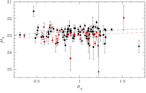
Figure 7.— GCLF turnover magnitude, $\mu_{z}$, vs. GCLF dispersion, $\sigma_{z}$, both inferred from Gaussian fits to the $z$-band data, for all the galaxies in the ACS Virgo (black symbols) and Fornax (red symbols) cluster surveys. The sample has been morphologically separated into elliptical (circles), lenticular (triangles), and dwarf (squares) galaxies. The lines represent a simultaneous error-weighted linear fit to the data corresponding to $\mu_{z}=(22.99\pm 0.04)-(0.23\pm 0.04)\sigma_{z}$, with an offset of $\Delta\mu_{z}=0.21\pm 0.04$ for the Fornax data.

The observed difference between SBF and GCLF distances has already been reported by Richtler (2003), attributing this phenomena to the presence of intermediate-age GCs, which might contaminate the sample. Our sample is made up exclusively of early type galaxies, which are old stellar systems where the presence of intermediate-age clusters is rarely observed (although some cases have been reported in the literature, see e.g. Goudfrooij et al. 2001 for the case of NGC1316 = FCC21, and Puzia et al. 2002 for NGC4365 = VCC731), so it is unlikely that this is the reason of the observed discrepancy. Ferrarese et al. (2000a) have consistently reported discrepancies between their GCLF estimated distances and those obtained from other estimators (particularly SBF and PNLF). They found the GCLF turnover in Fornax to be a full 0.5mag brighter than the value observed in Virgo. The internal errors in the GCLF measurements and the expected uncertainty due to cluster depth effects were not found to be enough to explain the scatter in their observations, suggesting the existence of a second parameter driving the GCLF turnover magnitude.

One obvious way to explain the observed discrepancy between GCLF and SBF measurements would be a mean age difference for the Virgo and Fornax cluster galaxies (i.e., the Fornax cluster galaxies might be younger by some amount, leading to a brighter turnover). The key question, then, is determining the age difference that would be needed to explain the observed $\sim$0.23 mag difference. According to the Bruzual & Charlot (2003) models, for a metallicity of $Z=0.004$ and a Salpeter (1955) initial mass function, the observed offset would be consistent with an age of roughly 9 Gyr for the Fornax cluster when arbitrarily assuming an age of 12 Gyr for Virgo. This age difference would also translate into slightly bluer mean colors for the Fornax GCs, which should be on average $\sim$0.04 mag bluer than their Virgo counterparts at a fixed galaxy mass. Performing a linear fit to the GCs mean color $\langle g-z\rangle$ vs. M_z,gal correlation of our data we found that both clusters could follow the same trend but including an offset of $0.022\pm 0.015$ mag to redder colors in the case of Virgo. Although almost consistent with zero, this value is also consistent with the expected color discrepancy given by the necessary age difference. The SBF technique, in which the fluctuations are calibrated against a measure of the stellar populations (i.e., color), would have this difference, if real, accounted for.

5.3. The Observed Dispersion on the Value of $\mu_{z}$

A relatively large scatter can be observed in the turnover magnitude values displayed in Figure 6. In this subsection we want to address the question of how much of this dispersion is intrinsic to the sample and how much is the result of observational effects. The histograms in Figure 8 give a better illustration of this scatter, where we have plotted the distribution of magnitudes around the mean turnover magnitude of each sample, estimated though a 3-sigma clipping algorithm. Subtracting the mean turnover magnitudes of both samples we obtain: $(\bar{\mu}^{g}_{F}-\bar{\mu}^{g}_{V})=0.15$ mag and $(\bar{\mu}^{z}_{F}-\bar{\mu}^{z}_{V})=0.17$ mag, which delivers a first-order estimate of the relative Virgo-Fornax distance modulus. We estimate the observed dispersion on the right ($z$-band) panels of Figure 8 in 0.31 mag and 0.28 mag, for Virgo and Fornax respectively, also using a 3-sigma clipping algorithm. We are more interested on studying the dispersion on the $z$-band because is much less sensitive to metallicity variations than the $g$-band.

There are then three main factors driving the spread: cluster depth, measurement errors and the intrinsic scatter in the turnover magnitude. From their 3D map of the Virgo cluster, Mei et al. (2007) have determined that the back-to-front depth of the cluster measured from our sample of galaxies is 2.4$\pm$0.4 Mpc ($\pm 2\sigma$ of the intrinsic distance distribution). At the Virgo distance this translates into a dispersion due to line of sight effects of $\sim$0.075 mag. For the Fornax cluster, Blakeslee et al. (2009) estimated a depth of 2.0${}^{+0.4}_{-0.6}$ Mpc ($\pm 2\sigma$ of the distance distribution in the line-of-sight), equivalent to a dispersion of $\sim$0.05 mag. Therefore for both clusters, the observed dispersion is significantly higher than the one expected from the cluster depth only.

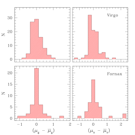
Figure 8.— Spread in magnitude around the weighted mean turnover magnitude, for Virgo (top) and Fornax (bottom) in the $g$ (left) and z (right) bands.

Given the observational errors and the known depths of the two clusters, we would like to determine whether there is any intrinsic dispersion in the value of $\mu$. In order to do that we simulated a distribution of N galaxies (with N being 89 and 43 for Virgo and Fornax respectively) with roughly the same intrinsic turnover magnitude (we included a slight trend in luminosity derived from the lower panel of Figure 9), and we assigned them a random distance by using a Gaussian depth distribution with appropriate width (0.075 mag for Virgo and 0.05 mag for Fornax). An additional random error was added to this distribution based on the observed uncertainties of our samples. The final distribution of magnitudes was then used to measure the dispersion of the simulated sample also by using a 3-sigma clipping algorithm. This procedure was iterated 10000 times for each sample, delivering a mean expected dispersion in the value of $\mu$ of 0.22 mag for Virgo, and 0.23 mag for Fornax. These values are lower than the dispersion measured in our samples, so we added an additional intrinsic dispersion term to the simulations until the observed dispersion was reached. This difference allows for an additional dispersion of 0.21 mag in the case of Virgo and 0.15 mag for the Fornax cluster, which can not be accounted by the cluster depth or the observational errors alone, and therefore corresponds to an intrinsic dispersion in the value of $\mu$.

The $z$-band histograms shown in Figure 8 are not symmetric around zero, a higher dispersion can be observed for positive values of $(\mu_{z}-\bar{\mu}_{z})$. This is consistent with the fact that the GCLF parameters will always be more precisely determined for galaxies with larger GC systems and they dominate the estimation of an error-weighted mean. As we will discuss in §6 low luminosity galaxies tend to show fainter turnover magnitudes and will be therefore located on the positive side in Figure 8, which combined with the larger uncertainty on the determination of $\mu_{0}$ in these systems is responsible for the larger scatter for the positive values of $(\mu_{z}-\bar{\mu}_{z})$. We stress that, as mentioned above, in the simulations done to estimate the intrinsic dispersion this slight trend of $\mu$ with $M_{z,gal}$ is taken into account.

6. The Universality of $M_{TO}$

The use of the GCLF as a distance indicator is based on the assumption of a universal value of $M_{TO}$, which has indeed been shown to be fairly constant (within $\pm$0.2 mag for massive galaxies) for a wide range of galaxy environments. The precision and quantity of our observations allow to probe for potential dependencies of $M_{TO}$ on factors such us the luminosity of the parent galaxy, Hubble type, mean color of the GC system, and environment, that might lurk in the observed first-order constancy of $M_{TO}$.

Probing for a dependence on Hubble type is important because the usual procedure is to use the Milky Way and M31 (both spiral galaxies) data in order to calibrate the GCLF in distant ellipticals. Our sample consists exclusively of early-type galaxies, so we cannot study the effect that the Hubble type might have on the value of $M_{TO}$. However, we will discuss this later from the point of view of the metallicity, as the differences in the GCLF as function of the Hubble type have been attributed to metallicity variations between the galaxies (Ashman et al., 1995). We will now address the influence of these factors on our observed non-universal GCLF.

6.1. Luminosity

The question of whether bright galaxies do have the same $M_{TO}$ as faint galaxies is particularly interesting to study now that the correlation between $\sigma$ and $M_{gal}$ has been clearly established. Whitmore (1997) has claimed that dwarf ellipticals have values of $M_{TO}^{V}$ which are roughly 0.3 mag fainter than bright ellipticals, which was previously also mentioned by Durrell et al. (1996). In principle this should not represent a problem for the use of the GCLF as a distance indicator, as the method is mostly concentrated on massive galaxies which can be traced to larger distances. Jordán et al. (2006, 2007b) have also noticed that the turnover mass is slightly smaller in dwarf systems ($M_{B}\geq-18$) compared to more massive galaxies (see also Miller & Lotz (2007), showing that this might be partly accounted for by the effects of dynamical friction.

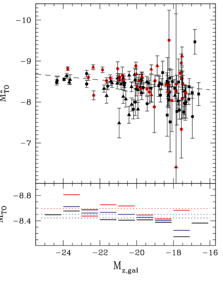
Figure 9.— Top: GCLF absolute $z$-band turnover magnitude ($M^{z}_{TO}$) derived from SBF distances (Blakeslee et al. 2009) vs. the absolute $z$-band magnitude of the parent galaxy ($M_{z,gal}$), for all the galaxies in the ACS Virgo (black) and Fornax (red) cluster surveys. The error-weighted linear fit corresponds to: $M^{z}_{TO}=(-7.66\pm 0.18)+(0.04\pm 0.01)M_{z,gal}$. The sample has been morphologically separated into elliptical (circles), lenticular (triangles), and dwarf (squares) galaxies. Bottom: Weighted mean turnover magnitude ($\bar{\textrm{M}}$${}^{z}_{TO}$) calculated in 1mag wide bins (continuous lines) and over the whole magnitude range (dotted lines), for the Virgo (black) and Fornax (red) sample. The blue lines also show the corresponding weighted mean values but using the combined sample.

We investigate a possible dependence of $\mu$ on $M_{z,gal}$ in Figure 9, which is equivalent to Figure 6 but with the observed turnover magnitudes now transformed to absolute turnover magnitudes using SBF distances (Mei et al. 2007, Blakeslee et al. 2009). The observed values of $\mu$ are relatively homogeneous in the range of $M_{z,gal}$ covered by our observations, between $M_{z,gal}\sim-24$ and $M_{z,gal}\sim-17$, however a tendency for dwarf galaxies to show slightly less luminous turnover magnitudes seems to be present. This tendency is characterized by the linear fit: $M^{z}_{TO}=(-7.66\pm 0.18)+(0.04\pm 0.01)M_{z,gal}$. The interpretation of this trend needs to be considered carefully because, due to their low luminosity, dwarf galaxies have smaller GC systems and the uncertainties on the determination of $\mu_{TO}$ are therefore higher. In order to lessen this problem, in the lower panel of Figure 9 we have plotted the weighted mean absolute magnitude in intervals of 1 magnitude compared to the weighted mean absolute magnitude calculated over the whole range of magnitudes. The lower luminosity bins tend to have mean magnitudes that are lower than the general mean both in each cluster and in the combined sample. At the lower luminosity bin (in the range between $-18<M_{z,gal}<-17$) the weighted mean absolute magnitude is 0.18 mag lower than the general value of -8.51, and 0.3mag lower than the most luminous bin (-24 $<M_{z,gal}<$ -23). From Figure 9 we can confirm then the trend suggested by Whitmore (1997) and reported by Jordán et al.(2006, 2007b), and we conclude that the luminosity (i.e. mass) of the parent galaxy has an effect on determining the peak of the GCLF, with fainter (lower-mass) galaxies having a fainter GCLF turnover.

Limiting the analysis to only the most massive galaxies in the sample ($M_{z,gal}<$ -21) we obtain an average turnover magnitude of $M_{z}=-8.53$ mag with a dispersion of 0.18 mag. These are the galaxies that could potentially be used as a distance indicator, and we can see here that they would deliver an accurate distance modulus estimation within the cosmic scatter of $\pm 0.2$ mag. There are nonetheless environmental dependencies that need to be considered before extending these findings to other systems because, as we can also observe from Figure 9, the galaxies in the Fornax cluster show absolute turnover magnitudes that are systematically brighter than the Virgo sample. We discus this point further in section §6.3.

6.2. Color

One of the most important requirements that a galaxy needs to fulfill in order to make feasible the use of its GCLF as a distance estimator is that its GC population must be old. The presence of an intermediate-age population will modify the GCLF by introducing clusters that will have brighter magnitudes than the older population.

The GC color distribution of our sample of 89 galaxies in Virgo was presented by Peng et al. (2006), where it was observed that on average galaxies at all luminosities in the samples ($-24<M_{z,gal}<-17$) appear to have bimodal or asymmetric GC color distributions. As discussed in Villegas et al. (2010, in preparation) the use of stellar population models allow us to discard large age differences between red and blue GCs if we assume that the mass distribution of GCs does not have a dependence on $[Fe/H]$ inside a given galaxy. With only a few exceptions, the population of blue and red GC appear to be coeval within errors for most of the galaxies, which lead us to concentrate on the problem of different metallicities between them. For giant ellipticals, this is also supported by previous observational studies (Puzia et al. 1999; Beasley et al. 2000, Jordán et al. 2002), although there are examples of massive galaxies that appear to have formed GCs recently triggered by mergers (e.g.  NGC 1316, Goudfrooij et al. 2001).

With the goal of obtaining an improved calibration for the value of $M_{TO}$, Ashman et al. (1995) studied the effects of metallicity on the GCLF showing that changes in the mean metallicity of the cluster sample produce a shift on $M_{TO}$, provided the mass distribution does not depend on [Fe/H]. According to Bruzual & Charlot (2003) models, the expected change in $z$-band turnover magnitude, $M^{z}_{TO}$, over the range of GC mean metallicity is $<$ 0.02 mag, which is utterly negligible considering the observational errors.

From a different point of view Figure 10 shows the correlation between turnover magnitude $\mu$ and mean GC color $\langle g-z\rangle$, in both $g$ (top) and $z$-band (bottom) for all the galaxies in the Fornax sample. From this plot it can be observed that on average $\mu_{g}$ remains constant as a function of $\langle g-z\rangle$, but $\mu_{z}$ tends to be brighter for redder GC systems. The interpretation of this plot presents a degeneracy between age and mass. If we assume that the Fornax galaxies, and by extension their GC systems, are all basically coeval, this trend can be explained by the fact that the $z$-band turnover better reflects mass (as it is only loosely dependent on metallicity), and therefore this is an indication that galaxies with lower masses (as accounted by the mean metallicity of its GC system) might have less-massive turnover values, which translates into fainter $\mu_{z}$. In the $g$-band, and as a consequence also in the nearby V-band, this effect is canceled by the fact that the mass-to-light ratio gets lower for GCs in lower-mass, lower-metallicity galaxies. Therefore the historically “constant turnover magnitude” of the V-band GCLF might just be a consequence of the incidental cancellation of these two factors at this wavelength.

Figure 10.— Turnover magnitude vs. mean GC color relationship for our Fornax cluster data in $g$ (top) and $z$-bands (bottom). The lines show the error weighted fit to the data and have a slopes of $0.13\pm 0.27$ in the $g$-band and $-1.01\pm 0.22$ in the $z$-band.

6.3. Environment

Even if we assume that the GC populations of galaxies of all morphological types are formed with the same initial mass function irrespective of available gas mass and metallicity, there is still the environmental factor to play against the existence of a universal GCLF. The particular media in which the clusters are formed might affect their evolution, shaping an environment-dependent GCLF.

Based on data from groups and clusters of galaxies Blakeslee & Tonry (1996) found evidence that $M_{TO}$ becomes fainter as the local density of galaxies increases. They used the velocity dispersion of groups of galaxies in the local universe as a density indicator in order to compare the values of $M_{TO}$ in different environments. Our data support the evidence presented by Blakeslee & Tonry (1996) in the sense they have also found a relative distance modulus that is too small compared to the SBF measurements. The trend of $M_{TO}$ changing as a function of environment (as accounted by velocity dispersion) is also followed by our data. However, it is important to mention that in spite of its lower velocity dispersion the Fornax cluster is denser than Virgo (Ferguson 1989b), and therefore the observed tendency seems to be more related to the total mass of the cluster than to local density.

Also, as discussed in §5.2 the observed discrepancy on the estimation of the relative Virgo-Fornax distance could be interpreted as a difference in mean-age between the stellar populations of these two clusters of galaxies, with an age difference of 3 Gyr being enough to explain this discrepancy. The combined use of high-resolution cosmological simulations and semi-analytic techniques (De Lucia et al. 2006) has shown that the faster evolution of protocluster regions produces star formation histories that peak at higher redshift for early-type galaxies hosted by more massive halos. This effect would therefore produce stellar populations in the Virgo clusters that are on average older when compared to stellar population belonging to a less massive galaxy cluster like Fornax. Mass estimates for Virgo vary substantially (e.g., $(0.15-1.5)\times 10^{15}\mathcal{M}_{\odot}$; Böhringer et al. 1994; Schindler et al. 1999; McLaughlin 1999; Tonry et al. 2000; Fouqué et al. 2001), but it is clear that its total mass is nearly an order of magnitude higher than the mass of Fornax ($\sim 7\times 10^{13}\mathcal{M}_{\odot}$, Drinkwater et al. 2001). The results presented by De Lucia et al. (2006) predict the expected mean-age difference for clusters of these masses to be $\sim$0.5 Gyr, a value that is too low to explain the observed difference in turnover magnitudes, but that is also dependant on the input parameters of the simulations.

7. Summary and Conclusions

We used ACS/HST data in order to study the GCLF of 89 early-type galaxies in the Virgo cluster and 43 galaxies in the Fornax cluster, which constitute the most homogeneous set of data used to date for this purpose. The GCLF of these galaxies was fitted by using a maximum likelihood approach to model the intrinsic Gaussian distribution after accounting for contamination and completeness effects. From the derived values of the turnover magnitude and the dispersion of the Gaussian fits we conclude that:

1. The analysis of 43 early-type galaxies belonging to the Fornax cluster shows that the dispersion of the GCLF decreases as the luminosity of the host galaxy decreases, confirming our previous results obtained with Virgo galaxies (Jordán et al. 2006, 2007b).

2. By using the GCLF turnover magnitude as a distance indicator on our homogeneous data set we derive a relative distance modulus between the Virgo and the Fornax clusters of $\Delta(m-M)_{\rm GCLF}=0.20\pm 0.04$ mag, which is lower than the one derived using SBF measurements on the same data, $\Delta(m-M)_{\rm SBF}=0.42\pm 0.03$ mag.

3. Setting the relative Virgo-Fornax distance as that given by SBF implies a difference in the value of $\langle\mu_{TO}\rangle$ in the two closest clusters of galaxies, suggesting that this quantity is influenced by the environment in which a GC system is formed and evolves. These results support a previous study by Blakeslee & Tonry (1996), who found a correlation between GCLF turnover magnitude and velocity dispersion of the host cluster, in the sense that galaxy clusters with higher velocity dispersions (higher masses) host galaxies with fainter turnovers in their GC systems.

4. The discrepancy in the absolute magnitude of the GCLF turnovers in Virgo and Fornax can be accounted for if GC systems in the Fornax clusters were on average $\sim$3 Gyrs younger than those in Virgo (thus making them brighter). Recent results from high-resolution numerical simulations (e.g. Springel et al. 2005, De Lucia et al. 2006) suggest that stellar populations of Virgo-like galaxy clusters (high mass and high velocity dispersion) were formed mostly at higher redshift compared to less massive and lower-dispersion clusters like Fornax. This trend could therefore be at least partially responsible for the observed discrepancy in the absolute GCLF turnover magnitudes between both clusters.

5. We have measured a total dispersion on the value of the turnover magnitude of 0.31 and 0.28 mag for Virgo and Fornax respectively. We show using simulations that these values can be only partially accounted by the dispersion produced by cluster depth and observational uncertainties. The additional dispersion can be modeled by an intrinsic dispersion on the value of $\mu_{0}$ of 0.21 mag for the Virgo cluster and 0.15 mag for Fornax.

6. The measured GCLF turnover is found to be systematically fainter for low luminosity galaxies, showing a $\sim$0.3 mag decrease on dwarf systems, although we suffer from large uncertainties in that galaxy luminosity regime. The luminosity (i.e. $\sim$ mass) of the parent galaxy seems to play an important role on shaping the final form of the luminosity distribution. This might be at least partly accounted for by the effects of dynamical friction if all other processes that contribute on shaping the mass function (two-body relaxation, tidal shocks, etc.) were to lead to a roughly constant M_TO (Jordán et al. 2007b).

7. Overall we find that GCLF parameters vary continuously and systematically as a function of galaxy luminosity (i.e. mass). The correlations we present here show no evidence for a dichotomy between giant and dwarf early-type galaxies at $M_{z}\sim-19.5$ ($M_{B}\sim-18$) in terms of their GC systems. This is consistent with results presented in several recent studies (e.g. Graham & Guzmán, 2003; Gavazzi et al. 2005, Côté et al., 2006), and is at odds with earlier claims by Kormendy (1985).

Table 1Gaussian GCLF parameters for all ACSVCS galaxies.

ID	$B_{gal}$	$\mu_{g}$	$\sigma_{g}$	$\mu_{z}$	$\sigma_{z}$	$\hat{\beta}$	$N$
(1)	(2)	(3)	(4)	(5)	(6)	(7)	(8)
VCC 1226	9.31	23.947 $\pm$ 0.066	1.340 $\pm$ 0.050	22.670 $\pm$ 0.063	1.304 $\pm$ 0.048	0.023	765
VCC 1316	9.58	23.872 $\pm$ 0.039	1.283 $\pm$ 0.030	22.591 $\pm$ 0.036	1.223 $\pm$ 0.028	0.014	1745
VCC 1978	9.81	23.893 $\pm$ 0.059	1.296 $\pm$ 0.046	22.636 $\pm$ 0.059	1.293 $\pm$ 0.046	0.022	807
VCC 881	10.06	23.887 $\pm$ 0.087	1.280 $\pm$ 0.068	22.775 $\pm$ 0.083	1.240 $\pm$ 0.066	0.034	367
VCC 798	10.09	23.889 $\pm$ 0.115	1.194 $\pm$ 0.078	22.760 $\pm$ 0.116	1.157 $\pm$ 0.080	0.012	370
VCC 763	10.26	23.874 $\pm$ 0.063	1.155 $\pm$ 0.050	22.759 $\pm$ 0.063	1.145 $\pm$ 0.049	0.035	506
VCC 731	10.51	24.343 $\pm$ 0.055	1.201 $\pm$ 0.043	23.166 $\pm$ 0.055	1.198 $\pm$ 0.043	0.021	907
VCC 1535	10.61	23.664 $\pm$ 0.087	1.107 $\pm$ 0.068	22.503 $\pm$ 0.086	1.091 $\pm$ 0.067	0.042	244
VCC 1903	10.76	23.405 $\pm$ 0.078	1.175 $\pm$ 0.063	22.214 $\pm$ 0.081	1.198 $\pm$ 0.065	0.046	308
VCC 1632	10.78	23.860 $\pm$ 0.089	1.400 $\pm$ 0.069	22.643 $\pm$ 0.086	1.374 $\pm$ 0.067	0.038	456
VCC 1231	11.10	23.710 $\pm$ 0.084	1.112 $\pm$ 0.065	22.571 $\pm$ 0.084	1.105 $\pm$ 0.065	0.058	254
VCC 2095	11.18	24.616 $\pm$ 0.321	1.669 $\pm$ 0.203	23.638 $\pm$ 0.363	1.693 $\pm$ 0.221	0.076	134
VCC 1154	11.37	23.887 $\pm$ 0.085	0.993 $\pm$ 0.066	22.763 $\pm$ 0.087	0.990 $\pm$ 0.067	0.065	192
VCC 1062	11.40	23.638 $\pm$ 0.114	1.208 $\pm$ 0.089	22.495 $\pm$ 0.112	1.187 $\pm$ 0.088	0.066	179
VCC 2092	11.51	24.030 $\pm$ 0.172	1.127 $\pm$ 0.133	22.923 $\pm$ 0.184	1.175 $\pm$ 0.139	0.114	92
VCC 369	11.80	23.609 $\pm$ 0.102	1.101 $\pm$ 0.079	22.414 $\pm$ 0.099	1.062 $\pm$ 0.079	0.068	179
VCC 759	11.80	23.803 $\pm$ 0.110	1.130 $\pm$ 0.089	22.687 $\pm$ 0.107	1.100 $\pm$ 0.086	0.067	172
VCC 1692	11.82	23.791 $\pm$ 0.123	1.051 $\pm$ 0.095	22.747 $\pm$ 0.135	1.099 $\pm$ 0.104	0.096	136
VCC 1030	11.84	23.711 $\pm$ 0.090	0.980 $\pm$ 0.070	22.595 $\pm$ 0.092	1.013 $\pm$ 0.071	0.072	176
VCC 2000	11.94	23.511 $\pm$ 0.107	1.201 $\pm$ 0.082	22.471 $\pm$ 0.104	1.163 $\pm$ 0.080	0.071	197
VCC 685	11.99	23.639 $\pm$ 0.121	1.236 $\pm$ 0.095	22.555 $\pm$ 0.120	1.210 $\pm$ 0.098	0.085	167
VCC 1664	12.02	23.665 $\pm$ 0.109	1.059 $\pm$ 0.085	22.472 $\pm$ 0.103	1.009 $\pm$ 0.083	0.092	146
VCC 654	12.03	23.991 $\pm$ 0.183	0.926 $\pm$ 0.135	23.056 $\pm$ 0.198	0.940 $\pm$ 0.152	0.194	48
VCC 944	12.08	23.708 $\pm$ 0.121	0.872 $\pm$ 0.093	22.651 $\pm$ 0.124	0.864 $\pm$ 0.097	0.132	91
VCC 1938	12.11	23.766 $\pm$ 0.133	1.076 $\pm$ 0.110	22.792 $\pm$ 0.128	1.009 $\pm$ 0.120	0.114	101
VCC 1279	12.15	23.645 $\pm$ 0.105	1.026 $\pm$ 0.079	22.621 $\pm$ 0.111	1.048 $\pm$ 0.085	0.097	138
VCC 1720	12.29	23.670 $\pm$ 0.127	0.797 $\pm$ 0.102	22.613 $\pm$ 0.143	0.870 $\pm$ 0.115	0.141	71
VCC 355	12.41	24.504 $\pm$ 0.279	1.208 $\pm$ 0.207	23.316 $\pm$ 0.206	1.027 $\pm$ 0.158	0.167	62
VCC 1619	12.50	24.261 $\pm$ 0.219	1.074 $\pm$ 0.161	23.166 $\pm$ 0.234	1.082 $\pm$ 0.171	0.165	66
VCC 1883	12.57	24.125 $\pm$ 0.187	1.135 $\pm$ 0.148	22.996 $\pm$ 0.166	1.064 $\pm$ 0.136	0.124	83
VCC 1242	12.60	23.731 $\pm$ 0.113	0.927 $\pm$ 0.088	22.636 $\pm$ 0.120	0.983 $\pm$ 0.093	0.105	116
VCC 784	12.67	24.269 $\pm$ 0.161	0.865 $\pm$ 0.123	23.102 $\pm$ 0.159	0.806 $\pm$ 0.131	0.179	64
VCC 1537	12.70	23.662 $\pm$ 0.240	0.977 $\pm$ 0.183	22.750 $\pm$ 0.309	1.124 $\pm$ 0.232	0.256	45
VCC 778	12.72	24.073 $\pm$ 0.178	1.052 $\pm$ 0.139	22.972 $\pm$ 0.172	1.009 $\pm$ 0.134	0.163	74
VCC 1321	12.84	24.160 $\pm$ 0.225	0.926 $\pm$ 0.168	23.153 $\pm$ 0.222	0.919 $\pm$ 0.166	0.198	50
VCC 828	12.84	23.804 $\pm$ 0.157	1.045 $\pm$ 0.142	22.787 $\pm$ 0.131	0.895 $\pm$ 0.113	0.143	80
VCC 1250	12.91	23.583 $\pm$ 0.145	0.815 $\pm$ 0.111	22.609 $\pm$ 0.154	0.831 $\pm$ 0.118	0.200	54
VCC 1630	12.91	24.124 $\pm$ 0.326	1.283 $\pm$ 0.232	23.104 $\pm$ 0.331	1.304 $\pm$ 0.230	0.217	57
VCC 1146	12.93	23.939 $\pm$ 0.141	0.970 $\pm$ 0.186	22.749 $\pm$ 0.127	0.890 $\pm$ 0.124	0.148	82
VCC 1025	13.06	24.251 $\pm$ 0.112	0.847 $\pm$ 0.097	23.335 $\pm$ 0.136	0.938 $\pm$ 0.110	0.143	104
VCC 1303	13.10	23.681 $\pm$ 0.140	0.821 $\pm$ 0.106	22.793 $\pm$ 0.139	0.805 $\pm$ 0.108	0.176	61
VCC 1913	13.22	23.688 $\pm$ 0.113	0.724 $\pm$ 0.103	22.675 $\pm$ 0.117	0.738 $\pm$ 0.102	0.181	65
VCC 1327 *	13.26	23.688 $\pm$ 0.121	1.262 $\pm$ 0.093	22.626 $\pm$ 0.115	1.212 $\pm$ 0.088	0.081	173
VCC 1125	13.30	23.667 $\pm$ 0.127	0.781 $\pm$ 0.109	22.645 $\pm$ 0.136	0.791 $\pm$ 0.109	0.179	62
VCC 1475	13.36	24.073 $\pm$ 0.141	0.990 $\pm$ 0.107	23.199 $\pm$ 0.178	1.101 $\pm$ 0.133	0.137	86
VCC 1178	13.37	23.609 $\pm$ 0.134	0.997 $\pm$ 0.102	22.562 $\pm$ 0.123	0.949 $\pm$ 0.090	0.124	90
VCC 1283	13.45	24.049 $\pm$ 0.152	0.894 $\pm$ 0.120	23.023 $\pm$ 0.167	0.932 $\pm$ 0.129	0.170	66
VCC 1261	13.56	23.962 $\pm$ 0.275	1.133 $\pm$ 0.208	23.004 $\pm$ 0.327	1.243 $\pm$ 0.238	0.217	46
VCC 698	13.60	23.793 $\pm$ 0.090	0.843 $\pm$ 0.066	22.777 $\pm$ 0.085	0.810 $\pm$ 0.062	0.105	119
VCC 1422	13.64	23.625 $\pm$ 0.169	0.656 $\pm$ 0.130	22.521 $\pm$ 0.168	0.651 $\pm$ 0.127	0.258	37
VCC 2048	13.81	23.450 $\pm$ 0.324	0.969 $\pm$ 0.217	22.420 $\pm$ 0.282	0.881 $\pm$ 0.194	0.420	22
VCC 1871	13.86	23.520 $\pm$ 0.608	1.181 $\pm$ 0.455	22.512 $\pm$ 0.604	1.154 $\pm$ 0.480	0.516	18
VCC 9	13.93	23.940 $\pm$ 0.391	1.086 $\pm$ 0.305	22.830 $\pm$ 0.260	0.894 $\pm$ 0.196	0.246	34
VCC 575	14.14	24.847 $\pm$ 0.271	0.665 $\pm$ 0.281	23.833 $\pm$ 0.130	0.333 $\pm$ 0.184	0.386	27
VCC 1910	14.17	23.758 $\pm$ 0.208	1.175 $\pm$ 0.161	22.630 $\pm$ 0.209	1.135 $\pm$ 0.176	0.180	60
VCC 1049	14.20	24.052 $\pm$ 0.257	0.550 $\pm$ 0.197	23.106 $\pm$ 0.396	0.634 $\pm$ 0.268	0.487	18
VCC 856	14.25	23.792 $\pm$ 0.185	0.887 $\pm$ 0.156	22.768 $\pm$ 0.164	0.862 $\pm$ 0.127	0.211	50
VCC 140	14.30	23.992 $\pm$ 0.245	0.790 $\pm$ 0.197	22.979 $\pm$ 0.249	0.822 $\pm$ 0.182	0.329	29
VCC 1355	14.31	24.554 $\pm$ 0.776	1.273 $\pm$ 0.541	23.682 $\pm$ 0.732	1.161 $\pm$ 0.530	0.471	20
VCC 1087	14.31	23.732 $\pm$ 0.134	0.926 $\pm$ 0.101	22.713 $\pm$ 0.133	0.898 $\pm$ 0.112	0.162	68
VCC 1297 *	14.33	23.403 $\pm$ 0.109	1.141 $\pm$ 0.082	22.299 $\pm$ 0.105	1.084 $\pm$ 0.080	0.092	152
VCC 1861	14.37	23.608 $\pm$ 0.222	1.015 $\pm$ 0.185	22.572 $\pm$ 0.206	0.937 $\pm$ 0.164	0.234	49
VCC 543	14.39	23.854 $\pm$ 0.196	0.692 $\pm$ 0.139	22.792 $\pm$ 0.184	0.635 $\pm$ 0.127	0.330	28
VCC 1431	14.51	24.092 $\pm$ 0.171	1.054 $\pm$ 0.128	23.054 $\pm$ 0.188	1.082 $\pm$ 0.140	0.158	71
VCC 1528	14.51	23.550 $\pm$ 0.137	0.720 $\pm$ 0.105	22.609 $\pm$ 0.129	0.697 $\pm$ 0.097	0.222	49
VCC 1695	14.53	24.416 $\pm$ 0.401	0.962 $\pm$ 0.289	23.480 $\pm$ 0.517	1.103 $\pm$ 0.357	0.380	22
VCC 1833	14.54	24.091 $\pm$ 0.223	0.695 $\pm$ 0.159	22.954 $\pm$ 0.147	0.500 $\pm$ 0.110	0.332	28
VCC 437	14.54	23.933 $\pm$ 0.162	0.783 $\pm$ 0.134	23.056 $\pm$ 0.167	0.845 $\pm$ 0.131	0.229	50
VCC 2019	14.55	23.551 $\pm$ 0.220	0.873 $\pm$ 0.200	22.619 $\pm$ 0.225	0.860 $\pm$ 0.193	0.303	34
VCC 200	14.69	24.459 $\pm$ 0.221	0.680 $\pm$ 0.144	23.582 $\pm$ 0.331	0.834 $\pm$ 0.221	0.381	25
VCC 571	14.74	24.392 $\pm$ 0.543	0.951 $\pm$ 0.346	24.249 $\pm$ 1.542	1.421 $\pm$ 0.810	0.478	17
VCC 21	14.75	24.073 $\pm$ 0.636	1.438 $\pm$ 0.418	22.963 $\pm$ 0.559	1.276 $\pm$ 0.387	0.351	26
VCC 1488	14.76	24.146 $\pm$ 0.303	0.580 $\pm$ 0.208	23.088 $\pm$ 0.390	0.553 $\pm$ 0.262	0.471	19
VCC 1499	14.94	24.562 $\pm$ 0.601	1.418 $\pm$ 0.377	23.489 $\pm$ 0.530	1.295 $\pm$ 0.341	0.272	35
VCC 1545	14.96	24.099 $\pm$ 0.164	0.910 $\pm$ 0.128	23.159 $\pm$ 0.183	0.930 $\pm$ 0.145	0.189	63
VCC 1192 *	15.04	23.781 $\pm$ 0.086	1.073 $\pm$ 0.066	22.663 $\pm$ 0.085	1.052 $\pm$ 0.064	0.064	213
VCC 1075	15.08	23.514 $\pm$ 0.169	0.554 $\pm$ 0.119	22.522 $\pm$ 0.155	0.515 $\pm$ 0.115	0.378	26
VCC 1440	15.20	24.267 $\pm$ 0.237	0.895 $\pm$ 0.176	23.270 $\pm$ 0.221	0.824 $\pm$ 0.162	0.259	38
VCC 230	15.20	23.941 $\pm$ 0.134	0.541 $\pm$ 0.106	23.078 $\pm$ 0.139	0.578 $\pm$ 0.105	0.274	38
VCC 2050	15.20	23.900 $\pm$ 0.118	0.281 $\pm$ 0.089	22.963 $\pm$ 0.135	0.304 $\pm$ 0.106	0.459	20
VCC 751	15.30	23.525 $\pm$ 0.191	0.504 $\pm$ 0.130	22.699 $\pm$ 0.206	0.509 $\pm$ 0.130	0.495	17
VCC 1828	15.33	23.807 $\pm$ 0.210	0.702 $\pm$ 0.183	22.757 $\pm$ 0.198	0.664 $\pm$ 0.148	0.355	27
VCC 1407	15.49	24.397 $\pm$ 0.123	0.665 $\pm$ 0.094	23.420 $\pm$ 0.144	0.745 $\pm$ 0.111	0.186	60
VCC 1886	15.49	23.034 $\pm$ 0.715	0.971 $\pm$ 0.463	21.565 $\pm$ 0.304	0.463 $\pm$ 0.215	0.622	14
VCC 1199 *	15.50	23.833 $\pm$ 0.094	1.166 $\pm$ 0.074	22.682 $\pm$ 0.089	1.125 $\pm$ 0.070	0.060	228
VCC 1539	15.68	23.813 $\pm$ 0.182	0.831 $\pm$ 0.168	22.820 $\pm$ 0.199	0.901 $\pm$ 0.147	0.275	43
VCC 1185	15.68	23.843 $\pm$ 0.172	0.693 $\pm$ 0.116	22.910 $\pm$ 0.155	0.639 $\pm$ 0.105	0.292	33
VCC 1489	15.89	23.977 $\pm$ 0.150	0.378 $\pm$ 0.129	23.157 $\pm$ 0.279	0.484 $\pm$ 0.469	0.417	22
VCC 1661	15.97	24.040 $\pm$ 0.281	0.630 $\pm$ 0.273	23.058 $\pm$ 0.285	0.614 $\pm$ 0.215	0.477	19

Table 2Gaussian GCLF parameters for all ACSFCS galaxies.

ID	$B_{gal}$	$\mu_{g}$	$\sigma_{g}$	$\mu_{z}$	$\sigma_{z}$	$\hat{\beta}$	$N$
(1)	(2)	(3)	(4)	(5)	(6)	(7)	(8)
FCC 21	9.4	26.350 $\pm$ 1.234	2.178 $\pm$ 0.059	25.150 $\pm$ 0.668	2.189 $\pm$ 0.060	0.011	647
FCC 213	10.6	24.090 $\pm$ 0.048	1.231 $\pm$ 0.038	22.802 $\pm$ 0.044	1.198 $\pm$ 0.035	0.015	1074
FCC 219	10.9	24.140 $\pm$ 0.072	1.110 $\pm$ 0.058	22.940 $\pm$ 0.072	1.112 $\pm$ 0.058	0.039	380
NGC 1340	11.2	24.384 $\pm$ 0.098	1.124 $\pm$ 0.074	23.468 $\pm$ 0.111	1.180 $\pm$ 0.082	0.039	280
FCC 167	11.3	24.023 $\pm$ 0.059	1.022 $\pm$ 0.046	22.808 $\pm$ 0.060	1.044 $\pm$ 0.047	0.026	424
FCC 276	11.8	24.032 $\pm$ 0.070	1.102 $\pm$ 0.063	22.960 $\pm$ 0.076	1.166 $\pm$ 0.061	0.040	361
FCC 147	11.9	24.077 $\pm$ 0.085	1.197 $\pm$ 0.067	22.894 $\pm$ 0.081	1.156 $\pm$ 0.064	0.047	320
IC 2006	12.2	24.076 $\pm$ 0.092	0.886 $\pm$ 0.070	22.935 $\pm$ 0.089	0.868 $\pm$ 0.067	0.085	132
FCC 83	12.3	24.026 $\pm$ 0.076	1.040 $\pm$ 0.058	22.906 $\pm$ 0.070	0.988 $\pm$ 0.054	0.044	274
FCC 184	12.3	23.956 $\pm$ 0.067	1.029 $\pm$ 0.054	22.664 $\pm$ 0.067	1.030 $\pm$ 0.054	0.042	306
FCC 63	12.7	24.023 $\pm$ 0.106	1.236 $\pm$ 0.084	22.951 $\pm$ 0.108	1.233 $\pm$ 0.086	0.058	231
FCC 193	12.8	23.934 $\pm$ 0.161	0.822 $\pm$ 0.123	22.830 $\pm$ 0.172	0.899 $\pm$ 0.130	0.176	48
FCC 153	13.0	24.066 $\pm$ 0.175	0.947 $\pm$ 0.135	23.086 $\pm$ 0.155	0.857 $\pm$ 0.119	0.161	60
FCC 170	13.0	24.016 $\pm$ 0.196	1.182 $\pm$ 0.167	23.073 $\pm$ 0.202	1.195 $\pm$ 0.171	0.137	71
FCC 177	13.2	23.897 $\pm$ 0.139	0.928 $\pm$ 0.108	22.923 $\pm$ 0.125	0.859 $\pm$ 0.095	0.129	70
FCC 47	13.3	23.993 $\pm$ 0.068	0.988 $\pm$ 0.053	22.948 $\pm$ 0.068	0.984 $\pm$ 0.054	0.044	276
FCC 43	13.5	24.342 $\pm$ 0.304	1.088 $\pm$ 0.238	23.261 $\pm$ 0.289	1.099 $\pm$ 0.220	0.208	37
FCC 190	13.5	23.934 $\pm$ 0.090	0.932 $\pm$ 0.072	22.937 $\pm$ 0.091	0.940 $\pm$ 0.073	0.071	156
FCC 310	13.5	24.144 $\pm$ 0.167	0.743 $\pm$ 0.122	23.184 $\pm$ 0.169	0.736 $\pm$ 0.123	0.229	39
FCC 148	13.6	23.851 $\pm$ 0.134	1.012 $\pm$ 0.107	22.837 $\pm$ 0.147	1.079 $\pm$ 0.117	0.111	86
FCC 249	13.6	23.913 $\pm$ 0.089	0.929 $\pm$ 0.068	22.935 $\pm$ 0.091	0.939 $\pm$ 0.070	0.078	155
FCC 255	13.7	23.737 $\pm$ 0.111	0.780 $\pm$ 0.089	22.714 $\pm$ 0.110	0.770 $\pm$ 0.087	0.125	80
FCC 277	13.8	24.244 $\pm$ 0.158	0.677 $\pm$ 0.136	23.278 $\pm$ 0.156	0.683 $\pm$ 0.121	0.199	42
FCC 55	13.9	24.446 $\pm$ 0.148	0.655 $\pm$ 0.111	23.441 $\pm$ 0.181	0.734 $\pm$ 0.135	0.223	37
FCC 152	14.1	23.485 $\pm$ 0.344	0.844 $\pm$ 0.234	22.492 $\pm$ 0.248	0.585 $\pm$ 0.179	0.456	16
FCC 301	14.2	24.383 $\pm$ 0.415	1.008 $\pm$ 0.289	23.605 $\pm$ 0.628	1.216 $\pm$ 0.406	0.353	21
FCC 335	14.2	23.026 $\pm$ 0.766	1.593 $\pm$ 0.585	21.954 $\pm$ 0.732	1.517 $\pm$ 0.570	0.525	14
FCC 143 *	14.3	23.873 $\pm$ 0.148	0.908 $\pm$ 0.114	22.929 $\pm$ 0.141	0.855 $\pm$ 0.119	0.158	62
FCC 95	14.6	24.154 $\pm$ 0.098	0.263 $\pm$ 0.074	23.069 $\pm$ 0.057	0.155 $\pm$ 0.046	0.373	21
FCC 136	14.8	23.968 $\pm$ 0.163	0.436 $\pm$ 0.245	23.011 $\pm$ 0.104	0.355 $\pm$ 0.088	0.294	25
FCC 182	14.9	24.169 $\pm$ 0.142	0.891 $\pm$ 0.111	23.220 $\pm$ 0.178	1.008 $\pm$ 0.136	0.145	59
FCC 204	14.9	24.192 $\pm$ 0.518	0.944 $\pm$ 0.392	23.599 $\pm$ 0.757	1.118 $\pm$ 0.498	0.443	17
FCC 119	15.0	25.464 $\pm$ 0.946	0.972 $\pm$ 0.551	25.150 $\pm$ 7.387	1.222 $\pm$ 0.312	0.411	17
FCC 26	15.0	23.208 $\pm$ 0.143	0.441 $\pm$ 0.114	22.394 $\pm$ 0.226	0.657 $\pm$ 0.159	0.337	22
FCC 90	15.0	23.953 $\pm$ 0.352	0.673 $\pm$ 0.299	23.026 $\pm$ 0.213	0.567 $\pm$ 0.211	0.370	21
FCC 106	15.1	23.966 $\pm$ 1.321	1.990 $\pm$ 0.917	23.235 $\pm$ 1.879	2.223 $\pm$ 1.326	0.486	15
FCC 19	15.2	24.552 $\pm$ 0.459	0.750 $\pm$ 0.291	23.483 $\pm$ 0.496	0.720 $\pm$ 0.320	0.463	16
FCC 288	15.4	24.913 $\pm$ 0.510	0.871 $\pm$ 0.353	24.355 $\pm$ 0.706	0.893 $\pm$ 0.682	0.426	17
FCC 202 *	15.3	23.996 $\pm$ 0.084	1.101 $\pm$ 0.068	22.834 $\pm$ 0.083	1.087 $\pm$ 0.069	0.050	232
FCC 324	15.3	23.698 $\pm$ 0.271	0.665 $\pm$ 0.207	22.947 $\pm$ 0.274	0.758 $\pm$ 0.192	0.384	21
FCC 100	15.5	24.119 $\pm$ 0.114	0.433 $\pm$ 0.098	23.366 $\pm$ 0.181	0.590 $\pm$ 0.137	0.272	34
FCC 203	15.5	24.155 $\pm$ 0.361	1.184 $\pm$ 0.270	23.167 $\pm$ 0.329	1.114 $\pm$ 0.241	0.271	30
FCC 303	15.5	23.479 $\pm$ 0.200	0.623 $\pm$ 0.141	22.531 $\pm$ 0.218	0.678 $\pm$ 0.152	0.350	22

Table 3Literature compilation of relative distance modulus between Virgo and Fornax clusters

Method	$\Delta(m-M)$	Reference
Cepheids	$0.47\pm 0.20$	1
Fund. Plane	$0.45\pm 0.15$	2
	$0.52\pm 0.17$	3
PNLF	$0.35\pm 0.21$	4, 5
	$0.30\pm 0.10$	6
GCLF	$0.08\pm 0.09$	7
	$0.13\pm 0.11$	8
	$0.09\pm 0.27$	6
	$0.17\pm 0.28$	9
SBF	$0.42\pm 0.03$	10

References

- Ashman (1995) Ashman, K.M., Conti, A., & Zepf, S.E., 1995, AJ, 110, 1164
- Beasley (2000) Beasley, M.A., Sharples, R.M., Bridges, T.J., Hanes, D.A., Zepf, S.E., Ashman, K.M., Geisler, D., 2000, MNRAS, 318, 1249
- Binggeli (1985) Binggeli, B., Sandage, A., & Tammann, G.A., 1985, AJ, 90, 1681
- Blakeslee (1996) Blakeslee, J.P. & Tonry, J.L., 1996, ApJ, 465, 19
- Blakeslee (1999) Blakeslee, J.P., Ajhar, E.A., & Tonry, J.L., 1999, in Post-Hipparcos Cosmic Candles, ed. A. Heck & F. Caputo (Boston: Kluwer), 181
- Blakeslee (2009) Blakeslee, J.P., Jordán, A., Mei, S., Ct̂é, P., Ferrarese, L., Infante, L., Peng, E.W., Tonry, J.L., West, M.J., 2009, ApJ, 694, 556
- Bohringer (1994) Böhringer, H., Briel, U. G., Schwarz, R. A., Voges, W., Hartner, G., & Trumper, J. 1994, Nature, 368, 828
- Bruzual (2003) Bruzual, G. & Charlot, S., 2003, MNRAS, 344, 1000
- Brodie & Strader (2006) Brodie, J.P. & Strader, J., 2006, ARA&A, 44, 193
- Ciardullo (1998) Ciardullo, R., Jacoby, G.H., Feldmeier, J.J., Bartlett, R.E, 1998, ApJ, 492, 62
- Cote (2004) Côté, P., Blakeslee, J.P., Ferrarese, L., Jordán, A., Mei, S., Merritt, D., Milosavljevic, M., Peng, E.W., Tonry, J.L., & West, M.J., 2004, ApJS, 153, 223
- Cote (2006) Côté, P., Piatek, S., Ferrarese, L., Jordán, A., Merritt, D., Peng, E.W., Haşegan, M., Blakeslee, J.P., Mei, S., West, M.J., Milosavljević, M., Tonry, J.L., 2006, ApJS, 165, 57
- Cote (2007) Côté, P., Ferrarese, L., Jordán, A., Blakeslee, J.P., Chen, C.W., Infante, L., Merritt, D., Mei, S., Peng, E.W., Tonry, J.L. 2007, ApJ, 671, 1456
- DeLucia (2006) De Lucia, G., Springel, V., White, S.D.M., Croton, D., Kauffmann, G., 2006, MNRAS, 366, 499
- Djorgovski (1987) Djorgovski, S., Davis, M., 1987, ApJ, 313, 59
- D’Onofrio (1997) D’Onofrio, M., Capaccioli, M., Zaggia, S.R., Caon, N., 1997, MNRAS, 289, 847
- Dressler (1987) Dressler, A., Lynden-Bell, D., Burstein, D., Davies, R.L., Faber, S.M., Terlevich, R., Wegner, G., 1987, ApJ, 313, 42
- Drinkwater (2001) Drinkwater, M.J., Gregg, M.D., & Colless, M., 2001, ApJ, 548, L139
- Durrell (1996) Durrell, P.R., Harris, W.E., Geisler, D., & Pudritz, R.E., 1996, AJ, 112, 972
- Elmegreen (1997) Elmegreen, B.G., & Efremov, Y.N., 1997, ApJ, 480, 235
- Fall (1977) Fall, S. M. & Rees, M. J., 1977, MNRAS, 181, 37
- Fall (1985) Fall, S. M. & Rees, M. J., 1985, ApJ, 298, 18
- Fall (2001) Fall, S.M., Zhang, Q., 2001, ApJ, 561, 751
- Ferguson (1989a) Ferguson, H. C. 1989a, AJ, 98, 367
- Ferguson (1989b) Ferguson, H. C. 1989b, Ap&SS, 157, 227
- Ferrarese (2000a) Ferrarese, L., Mould, J.R., Kennicutt, R.C., Huchra, J., Ford H.C., Freedman, W.L., Stetson, P.B., Madore, B.F., Sakai, S., Gibson, B.K., Graham, J.A., Hughes, S.M., Illingworth, G.D., Kelson, D.D., Macri, L., Sebo, K., Silbermann, N.A. 2000a, ApJ, 529, 745
- Ferrarese (2000b) Ferrarese, L., Ford, H.C., Huchra, J., Kennicutt, R.C., Mould, J.R., Sakai, S., Freedman, W.L., Stetson, P.B., Madore, B.F., Gibson, B.K., Graham, J.A., Hughes, S.M., Illingworth, G.D., Kelson, D.D., Macri, L., Sebo, K., Silbermann, N.A., 2000b, ApJS, 128, 431
- Ferrarese (2006) Ferrarese, L., Côté, P., Jordán, A., Peng, E.W., Blakeslee, J.P., Piatek, S., Mei, S., Merritt, D., Milosavljević, M., Tonry, J.L., West, M.J., 2006, ApJS, 164, 334
- Fioc (1997) Fioc, M. & Rocca-Volmerange, B., 1997, A&A, 326, 950
- Fouque (2001) Fouqué, P., Solanes, J. M., Sanchis, T., & Balkowski, C. 2001, A&A, 375, 770
- Freedman (2001) Freedman, W.L., Madore, B.F., Gibson, B.K., Ferrarese, L., Kelson, D.D., Sakai, S., Mould, J.R., Kennicutt, R.C., Ford, H.C., Graham, J.A., Huchra, J.P., Hughes, S.M.G., Illingworth, G.D., Macri, L.M., Stetson, P.B., 2001, ApJ, 553, 47
- Gavazzi (2005) Gavazzi, G., Donati, A., Cucciati, O., Sabatini, S., Boselli, A., Davies, J., Zibetti, S., 2005, A&A, 430, 411
- Gieles (2006) Gieles, M., Larsen, S.S., Scheepmaker, R.A., Bastian, N., Haas, M.R., Lamers, H.J.G.L.M., 2006, A&A, 446, 9
- Graham (2003) Graham, A.W., & Guzmán, R., 2003, AJ, 125, 2936
- Gnedin (1997) Gnedin, O.Y. & Ostriker, J.P., 1997, ApJ, 474, 223
- Goudfrooij (2001) Goudfrooij, P., Alonso, M.V., Maraston, C. & Minniti, D., 2001, MNRAS, 328, 237
- Harris (1994) Harris, W.E., & Pudritz, R.E., 1994, ApJ, 429, 177
- Harris (2001) Harris, W.E., 2001, in Star Clusters, ed. L. Labhardt & B. Binggeli (Berlin: Springer), 223
- Harris (2009) Harris, W.E., Kavelaars, J.J., Hanes, D.A., Pritchet, C.J., Baum, W.A., 2009, AJ, 137, 3314
- Izenman (1991) Izenman, A.J., 1991, J. Am. Stat. Assoc., 86, 205
- Jacoby (1990) Jacoby, G.H., Ciardullo, R., Ford, H.C., 1990, ApJ, 356, 332
- Jacoby et al. (1992) Jacoby, G.H., Branch, D., Ciardullo, R., Davies, R.L., Harris, W.E., Pierce, M.J., Pritchet, C.J., Tonry, J.L., Welch, D.L., 1992, PASP, 104, 599
- Jordan (2002) Jordán, A., Côté, P., West, M.J. & Marzke, R.O., 2002, ApJ, 576L, 113
- Jordan (2004) Jordán, A., Blakeslee, J.P., Peng, E.W., Mei, S., Côté, P., Ferrarese, L., Tonry, J.L., Merritt, D., Milosavljevic, M., & West, M.J. 2004, ApJS, 154, 509
- Jordan (2006) Jordán, A., McLaughlin, D.E., Côté, P., Ferrarese, L., Peng, E.W., Blakeslee, J.P., Mei. S., Villegas, D., Merritt, D., Tonry, J.L., & West, M.J. 2006, ApJ, 651, L25.
- Jordan (2007a) Jordán, A., Blakeslee, J.P., Côté, P., Ferrarese, L., Infante, L., Mei, S., Merritt, D., Peng, E.W., Tonry, J.L. & West, M.J., 2007a, ApJS, 169, 213
- Jordan (2007b) Jordán, A., McLaughlin, D.E., Côté, P., Ferrarese, L., Peng, E.W., Mei. S., Villegas, D., Merritt, D., Tonry, J.L., & West, M.J. 2007b, ApJS, 171, 101
- Jordan (2009) Jordán, A., Peng, E.W., Blakeslee, J. P., Côté, P., Eyheramendy, S., Ferrarese, L., Mei, S., Tonry, J.L., West, M.J., 2009, ApJS, 180, 54
- Kelson (2000) Kelson, D.D., Illingworth, G.D., Tonry, J.L., Freedman, W.L., Kennicutt, R.C., Mould, J.R., Graham, J.A., Huchra, J.P., Macri, L.M., Madore, B.F., Ferrarese, L., Gibson, B.K., Sakai, S., Stetson, P.B., Ajhar, E.A., Blakeslee, J.P., Dressler, A., Ford, H.C., Hughes, S.M.G., Sebo, K.M., Silbermann, N.A., 2000, ApJ, 529, 768
- King (1966) King, I.R., 1966, AJ, 71, 64
- Kissler (1994) Kissler, M., Richtler, T., Held, E.V., Grebel, E.K., Wagner, S.J., Capaccioli, M., 1994, 1994, A&A, 287, 463
- Kohle (1996) Kohle, S., Kissler-Patig, M., Hilker, M., Richtler, T., Infante, L., Quintana, H., 1996, A&A, 309, 39
- Kormendy (1985) Kormendy, J. 1985, ApJ, 295, 73
- Kundu (2001) Kundu, A., Whitmore, B.C., 2001, 2001, AJ, 121, 2950
- Lamers (2006) Lamers, H.J.G.L.M. & Gieles, M. 2006, A&A, 455, L17
- McLaughlin (1999) McLaughlin, D. E., 1999, AJ, 117, 2398
- McLaughlin (2008) McLaughlin, D.E. & Fall, S.M., 2008, ApJ, 679, 1272
- McMillan (1993) McMillan, R., Ciardullo, R., Jacoby, G.H., 1993, ApJ, 416, 62
- Mei (2005a) Mei, S., Blakeslee, J.P., Tonry, J.L., Jordán, A., Peng, E.W., Côté, P., Ferrarese, L., Merritt, D., Milosavljevic, M., & West, M.J., 2005a, ApJS, 156, 113.
- Mei (2005b) Mei, S., Blakeslee, J.P., Tonry, J.L., Jordán, A., Peng, E.W., Côté, P., Ferrarese, L., West, M.J., Merritt, D., & Milosavljevic, M., 2005b, ApJ, 625, 121
- Mei (2007) Mei, S., Blakeslee, J.P., Côté, P., Tonry, J.L., West, M.J., Ferrarese, L., Jordán, A., Peng, E.W., Anthony, A., & Merritt, D., 2007, ApJ, 655, 144
- Miller (2007) Miller, B.W. & Lotz, J.M., 2007, ApJ, 670, 1074
- Peebles (1968) Peebles, P.J.E. & Dicke, R.H., 1968, ApJ, 154, 891
- Peng (2006a) Peng, E.W., Jordán, A., Côté, P., Blakeslee, J.P., Ferrarese, L., Mei, S., West, M.J., Merritt, D., Milosavljevic, M., & Tonry, J.L., 2006, ApJ, 639, 95
- Prieto (2006) Prieto, J.L. & Gnedin, O.Y., 2008, ApJ, 689, 919
- Puzia (1999) Puzia, T.H., Kissler-Patig, M., Brodie, J.P., & Huchra J.P., 1999, AJ, 118, 2734
- Puzia (2002) Puzia, T.H., Zepf, S.E., Kissler-Patig, M., Hilker, M., Minniti, D., Goudfrooij, P., A&A, 391, 453
- Richtler (2003) Richtler T., 2003, LNP Vol. 635: Stellar Candles for the Extragalactic Distance Scale, 635, 281
- Salpeter (1955) Salpeter, E.E., 1955, ApJ, 266, 713
- (70) Schlegel, D.J., Finkbeiner, D.P., & Davis, M., 1998, ApJ, 500, 525
- Secker (1992) Secker, J., 1992, AJ, 104, 1472
- secker (96) Secker, J. & Harris, W. E., 1993, AJ, 105, 1358
- Schindler (1999) Schindler, S., Binggeli, B., & Böhringer, H. 1999, A&A, 343, 420
- Springel (2005) Springel, V., White, S.D.M., Jenkins, A., Frenk, C.S., Yoshida, N., Gao, L., Navarro, J., Thacker, R., Croton, D., Helly, J., Peacock, J.A., Cole, S., Thomas, P., Couchman, H., Evrard, A., Colberg, J., Pearce, F., 2005, Nature, 435, 629
- Tonry (1988) Tonry, J. L., & Schneider, D. P. 1988, AJ, 96, 807
- Tonry (2000) Tonry, J. L., Blakeslee, J. P., Ajhar, E. A., & Dressler, A. 2000, ApJ, 530, 625
- Schlegel (1998) Schlegel, D.J., Finkbeiner, D.P. & Davis, M., 1998, ApJ, 500, 525
- Vesperini (2000) Vesperini, E., 2000, MNRAS, 318, 841
- Vesperini (2001) Vesperini, E., 2001, MNRAS, 322, 247
- West (1993) West, M.J., 1993, MNRAS, 265, 755
- Whitmore (1997) Whitmore, B. C. 1997, in The Extragalactic Distance Scale, ed. M. Livio, M. Donahue, & N. Panagia (Baltimore: STScI), 254