Correlation Energy and Entanglement Gap in Continuous Models

Abstract

Our goal is to clarify the relation between entanglement and correlation energy in a bipartite system with infinite dimensional Hilbert space. To this aim we consider the completely solvable Moshinsky’s model of two linearly coupled harmonic oscillators. Also for small values of the couplings the entanglement of the ground state is nonlinearly related to the correlation energy, involving logarithmic or algebraic corrections. Then, looking for witness observables of the entanglement, we show how to give a physical interpretation of the correlation energy. In particular, we have proven that there exists a set of separable states, continuously connected with the Hartree-Fock state, which may have a larger overlap with the exact ground state, but also a larger energy expectation value. In this sense, the correlation energy provides an entanglement gap, i.e. an energy scale, under which measurements performed on the 1-particle harmonic sub-system can discriminate the ground state from any other separated state of the system. However, in order to verify the generality of the procedure, we have compared the energy distribution cumulants for the 1-particle harmonic sub-system of the Moshinsky’s model with the case of a coupling with a damping Ohmic bath at 0 temperature.

PACS 03.65.-Ud, 03.67.-Mn

1 Introduction

The concept of entanglement has been recently considered by many authors in connection with several properties of the quantum systems and as a potential resource in quantum computation and information processing both in discrete and in continuous variable systems [1][2]. Moreover, entanglement has also been recognized to play an important role in the study of many particle systems [3] and experimental and theoretical studies have demonstrated that it can affect thermodynamical properties both of the quantum phase transitions in the condensed matter and in molecular systems [4] [5] [6]. However, most of the studies on the subject consider only finite dimensional Hilbert models, which is not the typical situation occurring in atomic/molecular physics. As pointed out in [2], the theory of the entanglement for the infinite dimensional setting is full of difficulties, which can be cured choosing suitable subsets of the density matrices. In particular, the von Neumann entropy is not a continuous function in the Hilbert space, and for any given state of finite entanglement, one can find at least another state closer as we want to the previous one in trace norm, which is infinitely entangled.

However, a new area of research has been opened by [6] [7] [8], where it was shown that the entanglement, even if it is not a quantum observable, can be used in evaluating the so-called correlation energy: that is the difference between the true eigenvalue energy of a given composite system of identical entities, with respect to that one prescribed by the Hartree - Fock (HF) method. In [9] the case of the formation of the Hydrogen molecule was discussed, and a qualitative agreement between the von Neumann entropy of either atom ( as a measure of the entanglement of formation of the whole system) and the correlation energy as functions of the inter-nuclear distance was shown. However, the extension of this idea to multi-atomic molecules and its effectiveness remains still unclear [8][9]. Actually, the correlation energy is an artifact of the approximation procedure, then it is not a physical observable and, by second, it can be modified by the adopted method of calculations. Nevertheless, since any other approximating disentangled state has also a larger energy expectation value with respect to the HF state, one is lead to look at the correlation energy as an entanglement gap in the sense of [7]. Adding any further correction term at the wave function has to decrease the energy expectation value to the Hamiltonian eigenvalue and increase the entanglement at the same time up to fill the gap, describing in such a way a peculiar domain in state space, around the exact one. Thus, the first aim is to quantify such a kind of relation, at least on a specific model, finding a quantitative expression of the entanglement in terms of the correlation energy of the ground state for a composite bipartite system. In order to have an analytically tractable example containing all the desired features, we treated with a family of two coupled harmonic oscillators [10] in 3 dimensions. The coupling constant of the two parts is in a one-to-one correspondence with the correlation energy and and with entanglement estimators. Viceversa, assuming that such a relation is invertible, and then an estimation of the correlation energy can be expressed in terms of the entanglement, one may ask how direct measurements on one of component subsystems can provide such quantities. To this aim we have found for the considered model an expression of the concurrence, in terms of the momenta of the 1-particle subsystem energy probability distribution, from the knowledge that the composite system is in its ground state. Thus we have an entanglement witness and an a priori estimation of the correlation energy. However, in concrete we have to be able to distinguish the energy probability distribution of the entangled state from any other yielded by a mixed state or a pure thermal state. First we give an upper bound to the environmental temperature, over which all our procedure losses validity. Then, we compared the distribution generated by coupling a single harmonic oscillator with an Ohmic bath at 0-Temperature, by the analysis of all energy distribution cumulants.

In Sec. 2 we briefly review the main properties of the model: its exact fundamental state, the HF approximation and the correlation energy. Sec. 3 for the fundamental state of the Moshinsky’s model we evaluate the von Neumann entropy and the concurrence in terms of the correlation energy. Since the concurrence can be expressed in terms of the dispersions of observable conjugated quantities, also the correlation energy takes a well defined physical meaning. A similar relation can be established for the fidelity. In Sec. 4 we prove the existence of a continuous manifold of pure separable states, containing the HF state, having an overlap with the exact ground state, which can be larger with respect to the former. In Section 5 we describe how the 1-particle energy probability distribution for the exact state of the model can be distinguished from that one for a single harmonic oscillator coupled with an Ohmic bath at 0-Temperature. Some final remarks are addressed in the Conclusions.

2 The Moshinsky’s Model

In order to evaluate how good the HF mean field method is in computing quantum states, Moshinsky proposed a simple, but non trivial, model of two coupled spin-$\frac{1}{2}$ harmonic oscillators in 3 dimensions in [10]. In dimensionless unities, the Hamiltonian of the model reads

$$\hat{H}=\frac{1}{2}\left(\hat{\vec{p}}_{1}^{2}+\hat{\vec{p}}_{2}^{2}+\hat{\vec{r}}_{1}^{2}+\hat{\vec{r}}_{2}^{2}\right)-\frac{1}{2}K\left(\hat{\vec{r}}_{1}-\hat{\vec{r}}_{2}\right)^{2},$$ (1)

where $\hat{\vec{r}}_{i}$ and $\hat{\vec{p}}_{i}$ denote the position and the momentum operators of the i-th particle, respectively. The constant $K$ parametrizes the interaction strength of a supplementary quadratic potential between the two oscillators (notice the difference of sign with respect to [10]). The model describes a system of two identical particles in the same harmonic potential, interacting by a smooth effective repulsive coupling, which is truncated at the second order in a Taylor expansion for small interparticle distances. Thus, we will dwell upon $0\leq K<1/2$, where the upper bound will correspond to a breaking of the model, since no bound states can exist. This signals that the model is far to be realistic and it is intended only as a toy model shaped to our aims.

The model energy spectrum is

$$E_{n,m}=\frac{3}{2}\left(1+\chi^{2}\right)+n+m\chi^{2},\quad m,\;n\in{\bf N}\cup\left\{0\right\}$$ (2)

where

$$\chi=(1-2K)^{\frac{1}{4}},$$ (3)

plays the role of effective coupling constant, parametrizing a sort of double well potential, with an increasingly higher (or wider) barrier for $\chi\rightarrow 0$. The normalized position wave function of the fundamental level is given by

$$\Psi_{0}\left({\vec{R}},{\vec{r}}\right)=\left(\frac{\chi}{\pi}\right)^{3/2}e^{-R^{2}/2}e^{-\chi^{2}r^{2}/2},$$ (4)

where the mean and relative positions

$${\vec{R}}=\frac{{\vec{r}}_{1}+{\vec{r}}_{2}}{\sqrt{2}},\qquad{\vec{r}}=\frac{{\vec{r}}_{1}-{\vec{r}}_{2}}{\sqrt{2}}$$ (5)

have been defined, respectively. In general the spectrum shows degeneracies, but the lowest level is always simple, except for $\chi=0$, i.e. for the limiting value of the coupling $K\rightarrow 1/2$. Moreover, crossings occur for higher eigenvalues at isolated points of $K$, but we are not interested to them. Finally, since the function (4) is symmetric in the interchange ${\vec{r}}_{1}\leftrightarrow{\vec{r}}_{2}$ , the total spin must be necessarily into the singlet state. Thus, the spinorial aspect of the problem is not relevant at this stage, and it can be ignored.

Applying the standard HF mean field approximation for the ground state of the Hamiltonian (1), one is led to the wave function

$$\Psi_{\rm{HF}}\left({\vec{R}},{\vec{r}}\right)=\pi^{-3/2}(1-K)^{3/4}e^{-(1-K)^{1/2}\left.\left(R^{2}+r^{2}\right)\right/2},$$ (6)

corresponding to the approximated eigenvalue

$$E_{\rm{HF}}=3(1-K)^{1/2}.$$ (7)

Defining the correlation energy ( positive, by Ritz’s theorem ) as

$$E_{\rm{corr}}=E_{\rm{HF}}-E_{0,0}=3\sqrt{1-K}-\frac{3}{2}\left(1+\sqrt{1-2K}\right).$$ (8)

Moreover, the explicit expression of the overlap (or the squared fidelity) between the exact and the HF wave function is

$$\left|\left\langle\Psi_{\rm{HF}}|\Psi_{0}\right\rangle\right|^{2}=\frac{64(1-K)^{3/2}(1-2K)^{3/4}}{\left(\left(1+\sqrt{1-K}\right)\left(1+\sqrt{1-2K}\right)-K\right)^{3}}\leq 1,$$ (9)

Thus, one can figure out that adding to the HF state further corrections, surely the estimation of the energy eigenvalue improves and the fidelity increases, but the simplest factorized expression in (6) will be lost. Differently to what happens in the approximated state, the two oscillators in the correct fundamental state are entangled. From analytic point of view this happens because of the different coefficients of ${\vec{R}}$ and ${\vec{r}}$ in the wave function (4). From a different point of view, one can see the expressions (4) and (6) as two distinct continuous curves in the Hilbert space, parametrized by $K$ (or $\chi$). They have only one common point at $K=0$. The main property of the latter curve is to contain only factorized states.

3 Entanglement Estimation

Since we are dealing with pure states, the entanglement estimator is the entanglement entropy, given in term of the von Neumann entropy

$$S_{\rm{vN}}\left[\hat{\rho}_{r}\right]=-\rm{Tr}\left[\hat{\rho}_{r}\,\log_{2}\hat{\rho}_{r}\right]=-\sum_{i}\mu_{i}\,{log}_{2}\left(\mu_{i}\right),$$ (10)

of the reduced to 1-particle density matrix $\hat{\rho}_{r}=\rm{Tr}_{2}\left[\hat{\rho}\right]=\rm{Tr}_{1}\left[\hat{\rho}\right]$, denoting by $\mu_{i}$ the corresponding eigenvalues.

On the other hand, the von Neumann Entropy $S_{\rm{vN}}$ satisfies the additive relation $S_{\rm{vN}}\left[\hat{\rho}\otimes\hat{\sigma}\right]=S_{\rm{vN}}\left[\hat{\rho}\right]\rm{}+\rm{}S_{\rm{vN}}\left[\hat{\sigma}\right],$ for any factorized density operator $\hat{\rho}\otimes\hat{\sigma}$. But this is precisely the structure of the reduced density matrix, which factorizes into positional and spinorial contribution, where the latter takes the form $\hat{\sigma}=\frac{1}{2}\,{\bf 1}$ for the singlet spin state. Thus, it contributes to an additive constant term (equal to 1), which measures only the equal uncertainty in attributing one of the two possible quantum states to each spin. Following the ideas in [11] for fermions, anti-symmetrizing the product of 1-particle orthogonal states into a spin stationary state contains all information about entanglement by definition. In conclusion, here we will compare only the contributions to the entanglement coming from the space configurations factor of the 2-particle fundamental state.

In the position representation the exact 2-particles density matrix $\hat{\rho}$ for the fundamental state (4) is given by the integral kernel

$$\rho_{0}\left({\vec{r}}_{1},{\vec{r}}_{2},{\vec{r}^{\prime}}_{1},{\vec{r}^{\prime}}_{2}\right)=\left(\frac{\chi}{\pi}\right)^{3}e^{-\left(R^{2}+R^{\prime 2}\right)/2}e^{-\chi^{2}\left(r^{2}+r^{\prime 2}\right)/2},$$ (11)

where the supplementary variables ${\vec{R}^{\prime}}$ and ${\vec{r}^{\prime}}$ are in analogy with (5). A similar expression holds for the $|\Psi_{\rm{HF}}\rangle$ state (6), where the density matrix is given by the product of gaussian normal distributions with the same variance. The consequences of such different structure can be seen also by the comparison of the 1-particle space distribution densities, which are given by

$$\rho_{01}\left({\vec{r}}\right)=\left(\frac{2\chi^{2}}{\pi\left(\chi^{2}+1\right)}\right)^{3/2}\,e^{-2\frac{\chi^{2}}{\chi^{2}+1}\;r^{2}},\;\rho_{\rm{HF1}}\left({\vec{r}}\right)=\frac{(1-K)^{3/4}}{\pi^{3/2}}e^{-\sqrt{1-K}\;r^{2}}.$$ (12)

Thus, because of the repulsive interaction, the exact average distance between the particles is larger than in the approximated estimation, being their ratio $\left(\frac{\sqrt{1-K}\left(1+\sqrt{1-2K}\right)}{2\sqrt{1-2K}}\right)^{1/2}$, with a divergence for $K\rightarrow\frac{1}{2}$ ($\chi\rightarrow 0$).

The exact 1-particle integral operator density matrix $\hat{\rho}_{r}=\int\rho_{r}\left({\vec{r}},\,{\vec{r}^{\prime}}\right)\;\cdot\;d\,{\vec{r}^{\prime}}$ has the kernel

$$\rho_{r}\left({\vec{r}},{\vec{r}^{\prime}}\right) = \left(\frac{2\chi^{2}}{\pi\left(\chi^{2}+1\right)}\right)^{3/2}$$ (13)

$$\exp\left[\frac{2\left(\chi^{2}-1\right)^{2}{\vec{r}}\cdot{\vec{r}}^{\prime}-\left(4\chi^{2}+\left(\chi^{2}+1\right)^{2}\right)\left({\vec{r}}^{2}+\,{\vec{r}}\,^{\prime 2}\right)}{8\left(\chi^{2}+1\right)}\right].$$

That can be rewritten in the usual gaussian form [4] [15]

$$\rho_{r}^{\left(\Delta p,\Delta q\right)}\left({\vec{r}},{\vec{r}^{\prime}}\right)=\left(\frac{1}{2\pi\Delta q^{2}}\right)^{3/2}\exp\left[-\frac{1}{2}\left(\frac{\left({\vec{r}}+{\vec{r}}^{\prime}\right)^{2}}{4\Delta q^{2}}+\Delta p^{2}\left({\vec{r}}-{\vec{r}}^{\prime}\right)^{2}\right)\right],$$ (14)

where the squared mean values for the 1-particle position and momentum

$$\Delta q^{2}=\frac{\chi^{2}+1}{4\chi^{2}}\;,\qquad\Delta p^{2}=\frac{1}{4}\left(\chi^{2}+1\right),$$ (15)

have been introduced.

The system becomes disentangled when the 1-particle state is the pure minimal packet, i.e. when $\Delta p^{2}\Delta q^{2}=\frac{1}{4}$. But this occurs only for $K=0$ ($\chi=1$). In this sense $\Delta p^{2}$ and $\Delta q^{2}$ contains information about the entanglement of the system, as remarked in [4]. However, differently from [4], by the simple algebraic relation $\chi^{2}=\frac{\Delta p^{2}}{\Delta q^{2}}$ the squared mean values contain also information about the form and the strength of the interaction. Thus, one would arise the question if the analysis of (14) not only provides information about an entangled harmonic oscillator, but also the main properties of the coupling: is it coupled to a small system or to a thermodynamic bath?

From expression (13) the kernel of the eigenvalue equation for $\hat{\rho}_{r}$ is symmetric and of Hilbert-Schmidt type, since the coefficient of ${\vec{r}}^{\;2}$ (and ${\vec{r}}\,^{\prime\;2}$ ) is negative. So the spectrum is real and discrete, as for the tensor product of three independent oscillators. Accordingly, the eigenfunctions of $\hat{\rho}_{r}$ can be factorized in the product of three functions, each of them depending only on one real variable and the eigenvalues as a product

$$u_{l,m,n\rm{}}\left({\vec{r}}\right)=w_{l}(x)w_{m}(y)w_{n}(z),\qquad\mu_{l,m,n}=\nu_{l}\nu_{m}\nu_{n},$$ (16)

so that the problem is reduced to solve the 1-dimensional integral spectral problem

$$\int{\rho}_{r}(x,x^{\prime})\;w_{l}(x^{\prime})\;dx^{\prime}\;=\;\nu_{l}\;w_{l}(x),$$ (17)

which has the non degenerate spectrum and eigen-solutions of the form

$$\nu_{l}=Cc^{l},\qquad w_{l}(x)=H_{l}\left(\sqrt{\chi}x\right)\;e^{-\frac{\chi}{2}\;x^{2}},$$ (18)

where $C=\frac{4\chi}{\left(1+\chi\right)^{2}},\quad c=\left(\frac{1-\chi}{1+\chi}\right)^{2}$ and $H_{l}\left(\sqrt{\chi}x\right)$ denote the Hermite polynomials. Of course, these positive eigenvalues sum up to 1, because they are related to a matrix density operator. On the other hand, accordingly to (16) the eigenvalues of the one-particle density matrix $\hat{\rho}_{r}$ are given by

$$\mu_{k}=C^{3}c^{l+m+n}=C^{3}c^{k},\;k\,\epsilon\,{\mathbf{N}}_{0},$$ (19)

with degeneration order $\deg\left[\mu_{k}\right]=k\left(k+3\right)/2+1$ . Thus, the 1-particle density $\rho_{01}\left({\vec{r}}\right)=\sum_{lmn}C^{3}c^{l+m+n}\,|w_{l}\left(x\right)w_{m}\left(y\right)w_{n}\left(z\right)|^{2}$ is represented as a mixed state in the basis of the ”natural orbitals”, using the terminology by Lödwin [12], which describe a 3D single harmonic oscillator of frequency $\chi$. The weights $\mu_{k}$ describe a system at the equilibrium temperature $k_{B}T^{*}=3\chi/(2\ln\frac{1+\chi}{1-\chi})$, which is a decreasing function of $\chi$. Since experiments are always performed at a finite temperature, performing particle position/momentum measurements on such a system we need to work at $T<T^{*}\left(\chi\right)$, in order to highlight the quantum behavior discussed here.

For comparison, the spectrum of the reduced density matrix in the the HF approximation is given by $\left\{1\;\rm{(simple)},0\;\rm{(infinitely\;many\;degenerate)}\right\}$, with the corresponding eigenfunctions (for each of the three space variables) $\left\{H_{l}\left(\left(1-K\right)^{1/4}x\right)\exp\left[-\frac{\left(1-K\right)^{1/2}}{2}x^{2}\right]\right\}$.

Hence, if we are allowed to look at the eigenvalues of the density matrix operator $\hat{\rho}_{r}$ as the probabilities to find the 1-particle subsystem in one of the states of a ${K}$-parametrized family of harmonic oscillators, for small $K$ it can be found very likely in the fundamental one. But this probability decreases rapidly to 0 for $K\rightarrow{\scriptstyle{\frac{1}{2}}}$, while the higher states become significantly more accessible. Notice that at $K={\scriptstyle{\frac{1}{2}}}$ the system is meaningless, since all eigenvalues of $\hat{\rho}_{r}$ become 0 except one. However, for $0\leq K<{\scriptstyle{\frac{1}{2}}}$ one can analytically sum up $Tr\left(\hat{\rho}_{r}\right)=1$ pointlike, taking into account the degeneracy. On the other hand, the lack of coherence can be estimated also by computing the $Tr[\hat{\rho}_{r}^{2}]$, which is $1$ only for pure states. In the present case one has explicitly

$$\rm{Tr}\left[\hat{\rho}_{r}^{2}\right]=\frac{8\chi^{3}}{\left(1+\chi^{2}\right)^{3}},$$ (20)

which is a monotonically decreasing from $1$ to $0$ function on ${K}$.

Complementary to this quantity there is the so-called linear entropy [13], analogous to the concurrence [14]

$${\cal{C}}\left[\hat{\rho}_{r}\right]=1-\mbox{Tr}[{\hat{\rho}}_{r}^{2}],$$ (21)

which takes values in the range $\left[0,1\right]$. It is invariant under local unitary transformations on the separate oscillators (reduced to changes of phases). This entanglement estimator seems to be quite useful in the present case, since it is always bounded, even if it is defined on an $\infty$-dimensional Hilbert space.

The entropy of entanglement (10) can be explicitly written as

$$\!\!\!\!\!\!\!\!\!\!\!\!\!\!\!\!\!\!\!S_{\rm{vN}}\left[\hat{\rho}_{r}\right]=\frac{3}{\ln 4\;\chi}\left[\left(\chi+1\right)^{2}\ln\left(\chi+1\right)-2\chi\,\ln 4\chi-\left(\chi-1\right)^{2}\ln|\chi-1|\right].$$ (22)

For $K\rightarrow\frac{1}{2}$ ($\chi\rightarrow 0$), the entropy $S_{\rm{vN}}\left[\hat{\rho}_{r}\right]$ is logarithmic divergent, according to the expansion

$$S_{\rm{vN}}\left[\hat{\rho}_{r}\right]\approx-\frac{3\;\ln\left[\chi\right]}{\ln\left[2\right]}+O\left(1\right).$$ (23)

This is a well known result for harmonic chains [15], indicating the degeneracy of the ground state in the considered limit.

On the other hand, the behavior of $S_{\rm{vN}}\left[\hat{\rho}_{r}\right]$ near $K\rightarrow 0$ can be described by its series expansion

$$S_{\rm vN}\left[\hat{\rho}_{r}\right]=-\frac{3K^{2}\left(1+2K\right)}{8\,\ln(2)}\,\ln(K)+O\left(K^{2}\right),$$ (24)

approaching 0, because of the oscillators decoupling. However, this approximation becomes inaccurate very rapidly. From the above expression, for $K\rightarrow 0$, the asymptotic behavior of the entropy is controlled by a logarithmic term, differently from the correlation energy (8), which has a pure power expansion. Then, we cannot expect a great similarity between the two functions, also at very small values of $K$. This results breaks the conjectured existence of a simple relationship between the two quantities. On the other hand, let us observe that both functions $S_{\rm{vN}}[\hat{\rho}_{r}]$ and $E_{\rm{corr}}$ are monotonically increasing in $K$. Thus, the entanglement is an increasing function of the correlation energy (see Fig. 1). In order to have analytic expressions, we solve algebraically the coupling constant in terms of $E_{\rm{corr}}$ as

$$\chi\left(E_{\rm{corr}}\right)=\left[{1-\frac{4}{9}\left(\sqrt{2E_{\rm{corr}}\left(E_{\rm{corr}}+3\right)\left(2E_{\rm{corr}}+3\right)^{2}}-3E_{\rm{corr}}\left(E_{\rm{corr}}+3\right)\right)}\right]^{1/4}$$ (25)

and replacing into $S_{\rm{vN}}[\hat{\rho}_{r}]$, we obtain a one-to-one correspondence $\tilde{S}_{\rm{vN}}(E_{\rm{corr}})$.

Figure 1: The entanglement as a function of the correlation energy for the Moshinsky’s model.

In particular, one can look for asymptotic expressions of the entanglement for small values of $E_{\rm{corr}}$, corresponding to small couplings. Indeed, including logarithmic corrections at the lowest order near $E_{\rm{corr}}\approx 0$, one obtains

$$\tilde{S}_{\rm{vN}}\left(E_{\rm{corr}}\right)\approx\frac{\left(1+\,\ln(6)-\ln\left(E_{\rm{corr}}\right)\right)}{2\,\ln(2)}E_{\rm{corr}}+O\left(E_{\rm{corr}}^{3/2}\right),$$ (26)

for the Moshinsky’s oscillators. One verifies that similar expressions can be obtained studying other systems (for instance the 2-points Ising model), but up to now does not exist a general procedure to compute directly the coefficients appearing in the above developments. Moving to the upper limit $K\rightarrow 1/2$ ($\chi\rightarrow 0$), or equivalently $E_{\rm{corr}}\rightarrow\overline{E_{\rm{corr}}}=\frac{3}{2}\left(-1+\sqrt{2}\right)$, the entropy diverges logarithmic as

$$\tilde{S}_{\rm{vN}}\left(E_{\rm{corr}}\right)\approx-\frac{3\ln(\overline{E_{\rm{corr}}}-E_{\rm{corr}})}{\ln(4)}+O\left(1\right),$$ (27)

which is the specific behavior for degenerate ground state, as remarked for (23).

However, the singular behavior near 0 of the entanglement as a function of the correlation energy does not seem related to the specific way of its estimation. In fact, by using Eq. (25) into (20), as a function of the correlation energy the concurrence for the Moshinsky’s model takes the form

$${\cal{C}}\left(E_{\rm{corr}}\right)=1-\frac{24\,\sqrt{3}{{f}}^{3/4}}{\left(f^{1/2}+3\right)^{3}},$$ (28)

$$f=9+12\,E_{\rm{corr}}\left(E_{\rm{corr}}+3\right) -4\,\sqrt{2}\,\sqrt{E_{\rm{corr}}\left(E_{\rm{corr}}+3\right)\left(2E_{\rm{corr}}+3\right)^{2}},$$

a graph of which is shown in Fig. 2.

Figure 2: The entanglement expressed in terms of the concurrence as a function of the correlation energy for the Moshinsky’s model.

This function is regular in the origin, but it is not in its second derivative. Again a singularity is signaling a faster increase of the entanglement for small values of the correlation energy. But, the expression (28) is algebraic and it can be manipulated more easily. Specifically, for small values of the concurrence one gets the correlation energy as an half-integer power series of ${\cal{C}}$

$$E_{\rm{corr}}\approx{\cal{C}}+\sqrt{\frac{2}{3}}\,{\cal{C}}^{3/2}+\frac{2\,{\cal{C}}^{2}}{3}+O({\cal C}^{5/2}),$$ (29)

while for $0\ll{\cal{C}}\leq 1$ the expansion is

$$E_{\rm{corr}}\approx\overline{E_{\rm{corr}}}-\frac{3}{8}(1-{\cal C})^{2/3}+\frac{3}{64}\left(\sqrt{2}-4\right)(1-{\cal C})^{4/3}+O\left((1-{\cal C})\right)^{2}.$$ (30)

These expressions give direct relations between the correlation energy and the entanglement, which may suggest an experimental measure of the entanglement and of the correlation energy. In fact, let us suppose to perform two independent series of measurements of position and linear momentum on one particle of the system. Their results are distributed with squared mean values $\Delta q^{2}$ and $\Delta p^{2}$, respectively. On the other hand, by resorting to the relations (15) in terms of the coupling constant $\chi$ and to the expression (20), one gets

$$\mbox{Tr}\left[\hat{\rho}_{r}^{2}\right]=\left(\frac{\sqrt{\Delta p^{2}\,\Delta q^{2}}}{\frac{1}{2}\left(\Delta p^{2}+\Delta q^{2}\right)}\right)^{3}.$$ (31)

Thus the entanglement is related to the ratio between the uncertainty and the energy mean value of the observed subsystem. Furthermore, by the definition (21) and in the range of validity of expansion (29) (or (30) ), one may obtain a relation among observable quantities and the mathematical artifact $E_{\rm{corr}}$. On the other hand, relation (31) has to be used carefully since, if applied to a generic gaussian separate pure state, it does not give a measure of entanglement, of course. The point to be remarked is that its value depends by the special relation of the mean squared deviations on the coupling constant, not only on the preparation of the state.

Finally, the fidelity of the fundamental state of the Moshinsky’s model with the corresponding HF state or, equivalently, the overlap (9) can be expressed as a function of the entanglement. In some sense, we are comparing two different ways to measure the “distance” between the two curves of states, even if neither quantities actually have the properties of a distance. However, also in this case a monotonic function can be obtained for any pair of states corresponding to the same coupling constant $K$, or correlation energy $E_{\rm{corr}}$. This function is regular, even if at the extrema a singularity in its higher derivatives appears.

4 The gap of entanglement

Here we would like to elucidate the special role played by the HF state in the set of all separable states, which may be closer, in the sense of the trace - norm, to the exact solution. To this aim and since we are looking to a neighborhood of the ground state in the Hilbert space, let us restrict ourselves to the pure separable states, which are symmetric with respect to the change $1\leftrightarrow 2$ (the spins are into the singlet configuration) and generated by wavefunctions of the form

$$\tilde{\Psi}=\tilde{\Phi}\left(\vec{r}_{1}\right)\tilde{\Phi}\left(\vec{r}_{2}\right),$$ (32)

where for convenience we assume that $\tilde{\Phi}$ is normalized to 1. Of course, more general choices are possible, compatibly with the assumed identity of the particles. In the class of states (32) there exists the 1-parameter curve given by the gaussian functions

$$\tilde{\Psi}_{a}=\left(\frac{a}{\pi}\right)^{3/2}\exp\left[-\frac{a}{2}\left(R^{2}+r^{2}\right)\right],$$ (33)

certainly containing the HF wave function (6). Its overlap with the ground state (4) is such that

$$|\langle\tilde{\Psi}_{a}|\Psi_{0}\rangle|^{2}=\frac{64a^{3}\chi^{3}}{(a+1)^{3}\left(\chi^{2}+a\right)^{3}}\;\geq\;|\langle{\Psi}_{HF}|\Psi_{0}\rangle|^{2}$$ (34)

(see eq. (9)) for $a\in\left[a_{low}\left(\chi\right),\sqrt{\frac{1}{2}\left(\chi^{4}-1\right)+1}=\sqrt{1-K}\,\right]$. Of course, the upper bound is exactly the value involved in the HF wavefuction (see eq. (6)). The lower bound $a_{low}\left(\chi\right)$ is an algebraic positive monotonic increasing function, going from 0 to $\chi\rightarrow 0$, like $a_{low}\left(\chi\right)\approx\gamma\,\chi^{2}+O\left[\chi^{4}\right]$ ( $\gamma=const$) , to $1$ for $\chi\rightarrow 1$ ($K\rightarrow 0$), when the two extrema coincide. In particular, one sees that the maximum of overlapping is achieved for $a_{max}=\chi$, for which one has $|\langle\tilde{\Psi}_{a_{max}}|\Psi_{0}\rangle|^{2}=\frac{64\;\chi^{3}}{(\chi+1)^{6}}$, equal to 1 only at $\chi=1$ ($K=0$). It should be noticed that $a_{max}$ is exactly the same exponent appearing in the eigenfunctions of the 1-particle reduced density matrix operator (see eq. (18)), accordingly with the notion of ”natural orbital”. In conclusion, the HF state is not the closest (in the sense of the trace-norm) pure separable state to the exact fundamental state and one may wonder if other states arbitrarily close to it may be found. Of course, by deforming the pure gaussian form (33) with maximal overlapping, in the base of the Hermite polynomials one can construct symmetric factorized wavefunctions of the form

$$\tilde{\Psi}_{{\bf c}}=\prod_{i=1}^{3}N^{\left(i\right)}\left(\sum_{j=0}^{n_{i}}c_{j}^{\left(i\right)}H_{j}\left(\sqrt{\chi}x_{1}^{\left(i\right)}\right)\,\right)\left(\sum_{j=0}^{n_{i}}c_{j}^{\left(i\right)}H_{j}\left(\sqrt{\chi}x_{2}^{\left(i\right)}\right)\right)\tilde{\Psi}_{a_{max}},$$ (35)

for arbitrary complex constants $\left\{c_{j}^{\left(i\right)}\right\}$ and for suitable normalization constants $N^{\left(i\right)}$. Thus, it is not difficult to find

$$|\langle\tilde{\Psi}_{{\bf c}}|\Psi_{0}\rangle|^{2}=|\langle\tilde{\Psi}_{a_{max}}|\Psi_{0}\rangle|^{2}\prod_{i=1}^{3}\frac{|\sum_{j=0}^{n_{i}}2^{j}j!\,c_{j}^{\left(i\right)}{}^{2}\,\left(\frac{\chi-1}{\chi+1}\right)^{j}|^{2}}{\left(\sum_{j=0}^{n_{i}}2^{j}j!\,|c_{j}^{\left(i\right)}|^{2}\,\right)^{2}}.$$ (36)

The three factors in the r.h.s. of the above expression are $\leq 1$, then the overlapping of the generalized wave-packets (35) with the exact state cannot exceed the maximal one. In conclusion, we have proved that there exists a dense set of pure and separated states, containing the HF state, having overlap $|\langle\Psi_{HF}|\Psi_{0}\rangle|^{2}\leq|\langle\tilde{\Psi}|\Psi_{0}\rangle|^{2}<1$, except for $\chi=1$ ($K=0$), when $\Psi_{HF}\equiv\Psi_{0}$. Then, the exact state cannot be approached arbitrarily close by a separated state, except when it is itself separate. This result is complementary to the statement that entanglement entropy of a continuous model is a a discontinuous function, diverging at infinity in any neighborhood of any pure state [15]. The maximal overlapping is provided by taking the suitable tensor product of the natural orbitals [12]. Finally, because of the convexity of the set of all separable mixed states, i. e. of the form $\rho=\sum_{n}p_{n}|\tilde{\Psi}_{{\bf c}_{n}}\rangle\langle\tilde{\Psi}_{{\bf c}_{n}}|$, with $p_{n}\geq 0$ and $\sum_{n}p_{n}=1$, one can extend the previous statement to the entire space of states.

On the other hand, the HF state has been selected in the class of separable states by the minimal energy requirement. But in the domain of the pure separated states of form (33) the relation $\langle\widehat{H}\rangle_{\tilde{\Psi}_{a}}-E_{HF}=\frac{3\left(a-\sqrt{1-K}\right)^{2}}{2a}\;$ holds. Then, the expectation value of the Moshinsky’s Hamiltonian $\widehat{H}$ gets its absolute minimum indeed at the HF state. Moreover, this can be seen also considering general factorized states as in (35). Now, because of the convexity of the set of separable states, the minimum in the spectrum of a bounded observable from below is always achieved by a pure separable state. Thus, we conclude that the above introduced correlation energy is not simply a mathematical artifact, but it looks analogous to the concept of entanglement gap introduced in Ref. [7]. Since this is a global result, not depending on a particular computation procedure, we claim that the HF state for the Moshinsky’s model provides the minimum separable energy as introduced in [7] $E_{sep}=\min_{\rho_{separable}}Tr\left[\widehat{H}\rho_{separable}\right]=E_{HF}$. Moreover, the observable $Z_{EW}=\widehat{H}-E_{HF}{\bf 1}$ is an entanglement witness, the spectrum of which is non negative on all separable states and there exists the ground state (entangled) of the Moshinsky’s model for which its expectation value is $-E_{corr}<0$. Actually, for $\chi>0$ ($K<1/2$) isolated eigenvalues of $Z_{EW}$ may exist in the gap $\left[-E_{corr},0\right[$, but they corresponds to higher energy entangled states. Thus if in a measurement of $Z_{EW}$ we obtain a negative value, we can still affirm that the the system is in an entangled state, even if not necessarily in the ground state.

5 Entanglement Energetics

In the previous Sections we have shown that the entanglement gap is the main energetic scale that dictate if a composed system is, or not, entangled. For the Moshinsky’s model we have shown that this gap is given by the correlation energy, derived from the HF calculations. However, this relies on the full knowledge of the density matrix, while for pure states all needed information is encoded into the reduced matrix of a selected subsystem: in our case one of the harmonic oscillators. Thus the question if one can estimate the entanglement by energy measurements on the single harmonic oscillators arises, conditionally to the knowledge that the whole system is not in a separated ground state. These will be subjected to statistical fluctuations, which in principle contains the required information, i.e. the entanglement of original ground state of the composite system. This Section is devoted to how extract this result and how to distinguish the energy distribution of the entangled composite system, from the effects of couplings to a more generic environments, like an Ohmic bath, even if the latter is at 0 temperature.

First step concerns the calculation of the energy distribution for one single harmonic oscillator included into the Moshinsky’s model. To this aim it is useful to have the above expressions in the simple harmonic oscillator Hamiltonian eigenvector basis ${\cal B}=\left\{\varphi_{l,m,n}^{i}\right\}$ ( $i=1,2$).

First, the overlap of the exact wave function with a generic factorized state can be evaluated from the set of amplitudes

$$\langle\varphi_{l,m,n}^{1}\varphi_{l^{\prime},m^{\prime},n^{\prime}}^{2}|\Psi_{0}\rangle=\left(\frac{\chi^{1/2}}{\pi}\right)^{3}\frac{\emph{I}_{l,l^{\prime}}\emph{I}_{m,m^{\prime}}\emph{I}_{n,n^{\prime}}}{\sqrt{2^{l+l^{\prime}}2^{m+m^{\prime}}2^{n+n^{\prime}}l!l^{\prime}!m!m^{\prime}!n!n^{\prime}!}},$$ (37)

where the matrix $\left\{\emph{I}_{m,m^{\prime}}\right\}$ has a sort of chessboard structure, given by the relation

$$\emph{I}_{m,m^{\prime}}=2\pi\epsilon\left(m+m^{\prime}\right)\left(-1\right)^{m^{\prime}}\left(m+m^{\prime}-1\right)!!\left(1+\zeta\right)^{1/2}\zeta^{\frac{m+m^{\prime}}{2}},$$ (38)

where the expression $\zeta=\frac{1-\chi^{2}}{1+\chi^{2}}$ and the scaled step function $\epsilon\left(m\right)=\left\{\begin{array}[]{c}1/2\;\;m\;{\rm even}\\ 0\;\;\;\;m\;{\rm odd}\\ \end{array}\right.$ have been introduced.

On the other hand, in the basis ${\cal B}$ the amplitudes of $\tilde{\Psi}_{a}$ are given by

$$\langle\varphi_{l,m,n}^{1}\varphi_{l^{\prime},m^{\prime},n^{\prime}}^{2}|\tilde{\Psi}_{a}\rangle=\frac{a^{3/2}}{\pi^{3}}\frac{\emph{A}_{l}\emph{A}_{l^{\prime}}\emph{A}_{m}\emph{A}_{m^{\prime}}\emph{A}_{n}\emph{A}_{n^{\prime}}}{\sqrt{2^{l+l^{\prime}}2^{m+m^{\prime}}2^{n+n^{\prime}}l!l^{\prime}!m!m^{\prime}!n!n^{\prime}!}},$$ (39)

where

$$\emph{A}_{l}=\epsilon\left(l\right)2^{\,l+1+\frac{1}{2}}\alpha^{-l-1}\left(2-\alpha^{2}\right)^{l/2}\Gamma\left(\frac{l+1}{2}\right)$$ (40)

with $\alpha=\sqrt{1+a}$ for brevity. The expression (40) establishes that the non vanishing terms occur only for even principal quantum numbers $l,l^{\prime},\dots$, but they are not correlated among them.

In the representation (37)-(38) the elements of the full matrix density operator for the exact ground state are given by taking the tensor product in three dimensions of the 1-dimensional factors

$$\rho_{l,l^{\prime},m,m^{\prime}} = 4\left(1+\zeta\right)\chi\;\zeta^{\frac{l+l^{\prime}+m+m^{\prime}}{2}}$$

$$\frac{\left(-1\right)^{l^{\prime}+m^{\prime}}\;\varepsilon\left(l+l^{\prime}\right)\varepsilon\left(m+m^{\prime}\right)\left(l+l^{\prime}-1\right)!!\left(m+m^{\prime}-1\right)!!}{\left[2^{l+l^{\prime}+m+m^{\prime}}l!l^{\prime}!m!m^{\prime}!\right]^{1/2}}.$$

The corresponding reduced density matrix $\rho_{r,l,l^{\prime}}=\sum_{m}\rho_{l,m,l^{\prime},m}$ can be computed from the above expression, or using the continuous basis representation, contracting with respect the suitable states of the uncoupled harmonic oscillator. In particular, we are interested in the evaluation of the diagonal elements $\rho_{r,l,l}$, which represent the probabilities to find the 1-particle subsystem into the energy eigenstates of the uncoupled harmonic oscillator. It results that these quantities are related by the following recursion relation

$$\rho_{r,l+1,l+1}=\frac{l!}{\left(l+1\right)!}\chi\;\left(\zeta+1\right)\;\zeta^{l+1}\partial_{\zeta}\left(\frac{\rho_{r,l,l}}{\chi\;\left(\zeta+1\right)\zeta^{l}}\right)$$ (42)

with the expressions for the fundamental state

$$\rho_{r,0,0}=2\;\frac{\chi\;\left(\zeta+1\right)}{\sqrt{4-\zeta^{2}}}\;.$$ (43)

Thus, the general structure of the considered distribution is

$$\rho_{r,l,l}=2\zeta^{l}\frac{\chi\;\left(\zeta+1\right)}{\left(4-\zeta^{2}\right)^{\frac{2l+1}{2}}}\;Q_{l}\left(\zeta\right),$$ (44)

where $Q_{l}\left(\zeta\right)$ is a polynomial of degree $l$ in the ”scaled” coupling constant $\zeta$. This distribution of probability has its own peculiarities, which make it different from a generic factorized state or from a pure equilibrium thermodynamical distribution. Then, for comparison one computes the energy probability distribution for a factorized gaussian state by using the formulae (39) - (40). For each eigen-state label one obtains the expression

$$\rho_{r,l,l}=16a^{1/2}\frac{\varepsilon\left(l\right)^{2}\left(l-1\right)!!^{2}}{l!\left(a+1\right)\left(a+3\right)^{1/2}}\left(\frac{1-a}{1+a}\right)^{l}.$$ (45)

The first observation is that this distribution is different from 0 only for even $l$: this is a common character of all factorized gaussian states, included the HF approximated wave-packet, so it could be used to make an experimental comparison with the entangled state.

On the other hand, one can compute such a kind of quantity by the direct use of the 1-particle reduced matrix (14) [4]. In fact, by using the generating matrix for the Hermite polynomial, the diagonal elements of the reduced matrix in the basis of the pure harmonic oscillator are given by

$$\rho_{r,l,l}^{\left(\Delta p,\Delta q\right)}=2\frac{\left[\left(2\Delta p^{2}-1\right)\left(2\Delta q^{2}-1\right)\right]^{l/2}}{\left[\left(2\Delta p^{2}+1\right)\left(2\Delta q^{2}+1\right)\right]^{\left(l+1\right)/2}}P_{l}\left(\frac{4\Delta p^{2}\Delta q^{2}-1}{\sqrt{\left(4\Delta p^{4}-1\right)\left(4\Delta q^{4}-1\right)}}\right),$$ (46)

where $P_{l}$ denotes the $l$-th Legendre polynomial. The parameters $\Delta p$ and $\Delta q$ are independent quantities, limited only by the minimal uncertainty condition $\Delta p^{2}\Delta q^{2}\geq\frac{1}{4}$. Of course, substituting the expressions of $\Delta p$ and of $\Delta q$ given in (15), one recovers the formula (44): there the emphasis is on the dependency by the coupling strength. In Fig. (3) we give a set of contour plots of the probabilities to find the single harmonic subsystem ( of frequency $\omega=1$) in one of the first six eigenvalues as functions of the uncertainties $\left(\Delta p,\Delta q\right)$, accordingly to expression (46). The bold dashed curve is given by the equations (15) of the uncertainties in the Moshinsky’s model.

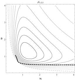
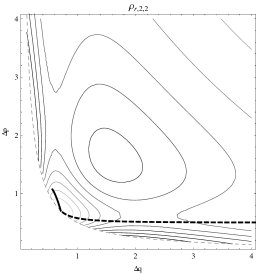
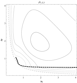
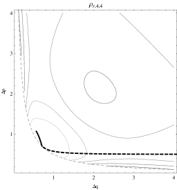
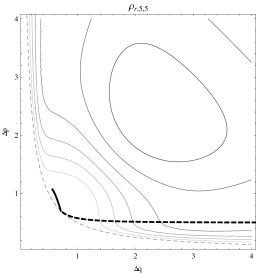
Figure 3: The probability distributions (46) to find into one of the first six modes of the simple harmonic oscillator a 1-particle subsystem, described by a reduced density matrix (14) in the $\left(\Delta q,\Delta p\right)$ plane. In the area between two contours the probability varies by $1/10$ of the maxima values $\{0.942809,0.249761,0.190042,0.105418,0.103428,0.0669486\}$, respectively for each plot, decreasing from black to lightest gray. The black thick dashed curve represents the values of $\left(\Delta q,\Delta p\right)$ given by (15), while the black thick continuous curve corresponds to the oscillator coupled to an Ohmic bath at $T=0^{o}$ accordingly to (50). The dashed gray boundary curve is determined by the hyperbola $\Delta q\Delta p=\frac{1}{2}$, which represents the gaussian factorized states. When the coupling constants of both models vanishes, the corresponding wave-packets are minimal.

Of course, the efficacy of the above procedure to measure the entanglement has to be evaluated by comparison with other situations. For instance, one may ask if is it possible to distinguish the above distribution of energy eigenvalues from a sufficiently general mixed one. Specifically we consider that one obtained coupling one of the harmonic oscillator to an Ohmic bath [16]. To this aim, we propose two different methods for this comparison.

The first way is based on the position and momentum measurements, from which we can reproduce the graph of Fig. 3, for fixed values of the coupling constant. In this case, the curves corresponding to the parametric representations of $(\Delta q,\,\Delta p)$ characterize the two models. Thus, we can distinguish the Ohmic model from the Moshinsky’s model by knowing the position and momentum uncertainty behaviour in the $(\Delta q,\,\Delta p)$ plane. Because of such measurements, this method produces a lack of information about the energetics of the system. Then, the second method, suggested by [4], is based on the analysis of the cumulants of the simple harmonic oscillator Hamiltonian $H_{HO}$, namely

$$\langle\langle H_{HO}^{n}\rangle\rangle=(-1)^{n}\left.\frac{d^{n}}{d\xi^{n}}\ln Z(\xi)\right|_{\xi=0},$$ (47)

where the partition function $Z(\xi)$ is evaluated by tracing the harmonic propagator in the imaginary time $\xi$, with respect the generic gaussian density matrix (14). Following the standard calculations [4] [17], one knows that

$$\!\!\!\!\!\!\!\!\!\!\!\!Z(\xi) = \langle e^{-\xi H_{HO}}\rangle_{\rho_{r}^{\left(\Delta p,\Delta q\right)}}=$$

$$\left[(\Delta p^{2}+\Delta q^{2})\sinh\xi+2\Delta q^{2}\Delta p^{2}(\cosh\xi-1)+\frac{1+\cosh\xi}{2}\right]^{-3/2}.$$

Then, a list of the cumulants can be algorithmically computed as polynomials of even dergee on the uncertainties $\left(\Delta q,\Delta p\right)$, as for instance

$$\!\!\!\!\!\!\!\!\!\!\!\!\!\!\!\!\!\ \langle\langle H_{HO}^{n}\rangle\rangle = \frac{3}{2}\left(\left(n-1\right)!\left(\Delta q^{2n}+\Delta p^{2n}\right)+O\left(\Delta q^{2\left(n-2\right)}+\Delta p^{2\left(n-2\right)}\right)\right),$$ (49)

For the Moshinsky’s model one substitutes the uncertainties given in (15) in (49), while for the Ohmic bath (in the underdamped limit) one uses the mean squared values [4]

$$\Delta q^{2}=\frac{1}{2\sqrt{1-\beta^{2}}}\left(1-\frac{2}{\pi}\arctan\frac{\beta}{\sqrt{1-\beta^{2}}}\right),$$

$$\Delta p^{2}=(1-2\beta^{2})\Delta q^{2}+\frac{2\beta}{\pi}\ln\frac{\omega_{C}}{\omega},$$ (50)

where $\beta$ is the coupling to the dissipative environment, in units of the oscillator frequency, and $\omega_{C}$ is a cutoff frequency.

In order to have a unique parameter, which measures the interaction strength between the singled out oscillator with the remaining of the composite system (the environment) in both considered cases, let us assume the relation

$$\beta=\frac{(1-\chi^{4})^{2}}{4(1+\chi^{4})}.$$ (51)

This relation is suggested by the derivation of the classical Langevin equation from a pure Hamiltonian system of coupled oscillators [16]. Thus, we can rewrite the above cumulants in terms of the coupling constant $\chi$ for both systems and compare them, as it has been shown in Fig. 4 for those of order 2.

Figure 4: The second energy cumulants $\langle\langle H_{HO}^{2}\rangle\rangle$ as a function of the coupling constant $\chi$ with $\omega_{C}=10\,\omega$. Dashed line represents the Ohmic bath, while solid line corresponds to system (1).

There, we can see that the two functions are similar for $\chi=1$, i.e. when they describe free harmonic oscillator in both cases. The situation dramatically changes when $\chi$ decreases, i.e. for stronger interactions. In fact, for $\chi\rightarrow 0$, the second energy cumulant associated with the Ohmic bath remains finite, while for the Moshinsky’s model it is divergent. Similar considerations can be made for the higher order cumulants. Thus, we have provided a method for distinguishing the two classes of states.

A different approach concerns the analysis the logarithm of the cumulants, at a fixed value of the coupling parameter $\chi$, as function of their order $n$. In fact, it results that $\ln\langle\langle H_{HO}^{n}\rangle\rangle$ is approximatively a linear function of $n$. But, from expression (49), the relevant physical information is contained in their slope and in the corresponding differences between the two models. Then, we introduce the function

$$R(\chi)=1-\frac{\left(\ln{\langle\langle H_{HO-Oh}^{n}\rangle\rangle}\right)_{\chi}}{\left(\ln{\langle\langle H_{HO-Mosh}^{n}\rangle\rangle}\right)_{\chi}},$$ (52)

which gives the relative difference of the $\ln\langle\langle H_{HO-J}^{n}\rangle\rangle$ ($J=Oh,\;Mosh$) slopes for the two models at different $\chi$ values (see Fig. 5). By inspection, we can deduce that for stronger or weaker interactions, i.e. for $\chi\approx 0$ or $\chi\approx 1$, the two models are well distinguishable. While this becomes less obvious for an intermediate range of the coupling constant, where the relative difference takes values $R(\chi)<0.5$.

Figure 5: The relative slope difference $R\left(\chi\right)$ as a function of the coupling constant $\chi$.

Finally, because of the explicit dependency of the cumulants from the position/momentum uncertainties, one may express the latter in terms of the first (mean energy) and second (variance) energy momentum. Thus, adopting the formula (31) as a common expression for any model of harmonic oscillator coupled to an environment, one provides a new expression of $\rm{Tr}\left[\hat{\rho}_{r}^{2}\right]$ as

$$\rm{Tr}\left[\hat{\rho}_{r}^{2}\right] = \left(\frac{\sqrt{8\langle\langle H_{HO}^{1}\rangle\rangle^{2}-12\langle\langle H_{HO}^{2}\rangle\rangle-9}}{2\langle\langle H_{HO}^{1}\rangle\rangle}\right)^{3}$$ (53)

and then of the concurrence only in terms of measured energy distribution properties. Moreover, from the arguments of Section 3 we get also an a priori estimation of the correlation energy. Now, using the parametrization of the coupling constant (51), one can compare the resulting concurrencies for the considered models (see Fig. 6). Qualitatively one can establish the intensity of the entanglement generated in those different models.

Figure 6: The concurrence for the Moshinsky’s model and the Ohmic model accordingly with the expression (53) as a function of the coupling constant $\chi$.

6 Conclusions

In the present article we have clarify the relation between the entanglement and correlation energy in a bipartite system with infinite dimensional Hilbert space. We have considered the completely solvable Moshinsky’s model of two linearly coupled harmonic oscillators, which may constitute a simple case before studying more complicated systems, like double well potentials. The system has a coupling constant, which can be varied in a finite range. Thus, it continuously parametrizes two special curves in the space states: one containing the exact ground states, the other the separable HF states. Of course, for vanishing coupling the two curves emerge from the same state, but their separation can be described in terms of norm, entanglement and energy correlation. The peculiarity of the second curve is to lie always in a set of 0 entropy entanglement states, while along the first one it increases monotonically (in $K$), with a logarithmic divergence when the ground state becomes degenerated. On the other hand, a similar description is given in terms of the correlation energy, which in principle is defined only for pairs of corresponding states (at the same coupling constant) in the two curves. We have proved that entanglement and correlation energy are one-to-one along these curves, at least for the considered model. However, they are not simply proportional, but at small couplings they have a quite different rate of increasing. This phenomenon occurs not only if one uses the entropy of entanglement for pure states, but also if one introduces the concurrence. However, in the considered model certain algebraic approximated expressions of the correlation energy in terms of the concurrence are given, so that an artifact of the calculation methods can take a physical interpretation. However, at the moment we have not a general method to compute directly the coefficients of such type of expansions. These could be very useful in order to have an alternative a priori estimation of the errors made in numerical computations of the correct expectation values of the energy. Such a type of relation may be useful in the studies of bipartite systems with many inner degrees of freedom, like the dimers of complex molecules (see [9] for instance). In this respect the explored concept of entanglement gap and its identification we made with the correlation energy may play an important role: it represents the energy range we have to be able to measure, in order to establish if a composed system is, or not, entangled. However, the theory of the entanglement gap for systems with infinite dimensional Hilbert space does not seem completely developed as for the finite dimensional case and further investigations are needed. In the final section we have shown that, conditionally to the knowledge that the whole system is not in a separated ground state, one can estimate the entanglement by energy measurements on the single harmonic oscillators. This can be done by two sequence of position and momentum measurements, as well by energy measurements. The distribution of the energy measurements is sufficiently characterized in terms of its cumulants. This analysis enable us to compare among different systems at 0 temperature and distinguish their ability to generate entanglement, for instance by using the parameter $R$ introduced in (52). Finally, via the formula (53) we propose a new estimator of the entanglement, based on the first two momenta of energy distribution of the considered subsystem. We plan to check the how good is the present approach in considering bipartite multi-particle systems and non linearly coupled systems. In particular, we would like to consider integrable systems, like in [18], in which a complete analytic control of the calculations is at the hand. Another direction of research is to consider a different entropy entanglement parameter, like the quantum version of the Tsallis entropy [19].

References

- [1] M.A. Nielsen and I.L. Chuang Quantum Computation and Quantum Information (Cambridge University Press, Cambridge, 2000)
- [2] J. Eisert and M.B. Plenio, Int. J. Quant. Inf. 1 (2003) 479
- [3] Y. Chen, P. Zanardi, Z.D. Wang and F.C. Zhang, New J. Phys. 8 (2006) 97
- [4] A.N. Jordan and M. Büttiker, Phys. Rev. Lett. 92 (2004) 247901
- [5] D.M. Collins, Z. Naturforsch. A 48 (1993) 68
- [6] Z. Huang and S. Kais, Chem. Phys. Lett. 413 (2005) 1
- [7] M.R. Dowling, A.C. Doherty and S.D. Bartlett, Phys. Rev. A 70 (2004) 062113
- [8] A. Mohajeri and M. Alipour, Int. J. Quant. Inf. 7 (2009) 801
- [9] T. Maiolo, F. Della Sala, L. Martina and G. Soliani, Theor. Math. Phys. 151 (2007) 1146
- [10] M. Moshinsky, Am. J. Phys. 36 (1968) 52
- [11] G.C. Ghirardi and L. Marinatto, Phys. Rev. A 70 (2004 ) 012109
- [12] P. - O. Löwdin, Phys. Rev. 97 (1955) 1474
- [13] F. Buscemi, P. Bordone and A. Bertoni, Phys. Rev. A 73 (2006) 052312
- [14] S. Hill and W.K. Wootters, Phys. Rev. Lett. 78 (1997) 5022; W.K. Wootters, Phys. Rev. Lett. 80 (1998) 2245
- [15] K. Audenaert, J. Eisert, M.B. Plenio and R.F. Werner, Phys. Rev. A 66 (2002) 042327
- [16] U. Weiss, Quantum Dissipative Systems (World Scientific, Singapore, 2008)
- [17] J. Zinn–Justin, Quantum Field Theory and Critical Phenomena (Clarendon Press, Oxford, 1993)
- [18] J.S. Dehesa, A. Martinez-Finkelshtein, V.N. Sorokin, J. Math. Phys. 44 (2003) 36
- [19] Xinhua Hu and Zhongxing Ye, J. Math. Phys. 47 (2006) 023502