Persistent memory for a Brownian walker in a random array of obstacles

Abstract

We show that for particles performing Brownian motion in a frozen array of scatterers long-time correlations emerge in the mean-square displacement. Defining the velocity autocorrelation function (VACF) via the second time-derivative of the mean-square displacement, power-law tails govern the long-time dynamics similar to the case of ballistic motion. The physical origin of the persistent memory is due to repeated encounters with the same obstacle which occurs naturally in Brownian dynamics without involving other scattering centers. This observation suggests that in this case the VACF exhibits these anomalies already at first order in the scattering density. Here we provide an analytic solution for the dynamics of a tracer for a dilute planar Lorentz gas and compare our results to computer simulations. Our result support the idea that quenched disorder provides a generic mechanism for persistent correlations irrespective of the microdynamics of the tracer particle.

1 Introduction

The essence of the Brownian motion of mesoscopic particles suspended in a solvent has been understood since the pioneering works of Einstein [1] and von Smoluchowski [2]. Today, Brownian motion constitutes a basic paradigm of stochastic processes [3, 4, 5] with applications in numerous fields, which may even utilize the noise as by stochastic resonance [6] and Brownian motors [7, 8, 9], not forgetting important generalizations beyond classical statistical physics to quantum Brownian system [10] and relativistic Brownian motion [11].

Following Einstein and von Smoluchowski, the statistics of the particle’s trajectories is described in terms of a probability distribution for the displacement as was measured shortly after by Perrin [12] relying on the newly developed dark field microscope. These displacements are cumulative, i.e., they are the sum of many small steps, and provided the steps are uncorrelated, the central limit theorem applies. Then for an unbiased random walk the probability cloud is described by a Gaussian which broadens as time proceeds. The corresponding trajectories are continuous but almost nowhere differentiable curves, self-similar in a statistical sense. This picture obviously cannot apply to the very small time and length scales where collisions with individual solvent molecules are resolved. Nevertheless it seems plausible that on a coarse-grained time and length scale all correlations due to these molecular processes are rapidly suppressed and Brownian motion emerges as mathematically described by a stochastic differential equation by Langevin [13] with a Wiener process as noise term.

This established picture had to be reconsidered when Alder and Wainwright [14, 15] showed in molecular dynamics simulations that the basic assumption of weakly correlated displacements is not fulfilled for the single particle motion in a fluid. Rather they found a long-time anomaly $Bt^{-d/2},B>0$ in the velocity autocorrelation function (VACF) due to the conservation of momentum in the fluid, where $d$ is the spatial dimension of the system. For a mesoscopic colloidal particle the direct experimental observation of these anomalies à la Perrin was achieved only 100 years after Einstein’s work using high-precision photonic force microscopy [16]. The power law correlations persist even in the presence of a bounding wall where momentum can be transferred to, although they decay more rapidly [17, 18, 19].

In this paper we argue that quenched disorder constitutes a second generic mechanism for persistent correlations in the velocity autocorrelation function. It was shown in the late 60s that in the Lorentz model, where a single tracer scatters ballistically in a random array of frozen hard obstacles, ring collisions lead to a nonanalytic dependence of the diffusion constant on the density of scatterers [20]. The same mechanism implies a power-law tail in the VACF [21] of the form $-At^{(d+2)/2}$, $A>0$. First, in contrast to Alder’s discoveries, the origin of this tail is not connected to momentum conservation, since the tracer exchanges momentum with the frozen scatterers. Second, the persistent correlation is negative reflecting the caging due to the obstacles. Here the correlations in the velocity are inherited from the configuration space since, loosely speaking, the particle remembers forever which paths are blocked by obstacles [22]. The predicted anomalies were soon partially confirmed by molecular dynamics simulations [23, 24] yet the prefactor of the tail was by an order of magnitude larger than expected. At higher densities the relaxation appears to become slower suggesting a density-dependent exponent [25, 26]. Later it was suggested that a second universal power law takes over as the the percolation threshold is approached [27] in qualitative agreement with a theoretical prediction obtained in a mode-coupling approach [28, 29]. The scenario of a crossover behavior explaining the enhanced prefactor of the power law was fully confirmed only recently [30].

Since the kinetic theory developed by Weijland and van Leeuwen [20] is rather involved, one is tempted to assume that their result constitutes a peculiarity of the Lorentz model with few general consequences. In this paper we show that the long-time anomalies in the VACF persist in a system where particles move diffusively rather than ballistically through the course of obstacles. We calculate analytically the first systematic correction for the complete scattering function and specialize to low wavenumbers to obtain the VACF. The long-time tail emerges again due to repeated encounters with the same scatterer, yet the derivation of this result drastically simplifies compared to the ballistic case, since a diffusive tracer finds the same obstacle many times without requiring the series of Boltzmann scattering events as the ballistic particle. We corroborate our analytic result by Brownian dynamics simulations in the dilute regime and discuss the range of validity of the low-density expansion. Last we conclude that frozen disorder generically entails long-time algebraic decay in the VACF irrespective of the microscopic dynamics implying that the basic assumption of quickly decaying correlations in Brownian motion is generally not fulfilled in heterogeneous media.

The notion of universal long-time anomalies also applies to hopping transport in disordered lattice models [31, 32] where again repeated encounters with the same scatterer lead to persistently correlated motion. There the VACF has been calculated up to second order in the obstacle density and the predictions have been nicely confirmed by computer simulation [33].

The paper is organized as follows. In Sec. 2, we briefly recall the main results of the anomalies in the low-density expansion of the ballistic Lorentz model. For the Brownian particle exploring a course of obstacles introduced in Sec. 3, a multiple scattering expansion is derived in Sec. 4 revealing that for the first-order density expansion it is sufficient to solve the single obstacle scattering problem. Section 5 calculates the corresponding forward scattering amplitude which is used in Sec. 6 to discuss the intermediate scattering function and, in particular, the velocity autocorrelation function in the dilute case. The analytic predictions are tested against computer simulation in Sec. 7. A summary of the results and conclusions are given in Sec. 8.

2 Ballistic Lorentz model and kinetic theory

In the Lorentz model randomly distributed, possibly overlapping obstacles of radius $\sigma$ represent a random, frozen environment in which a single, point-like tracer particle moves. The dynamics of the tracer is considered as ballistic with elastic scattering whenever an obstacle is encountered. In particular, energy is conserved and the particle’s velocity remains constant in magnitude for all times. Diffusion emerges after many collisions with the scatterer as the direction of the velocity is randomized. Since the obstacles are distributed randomly and independently, the structures are characterized solely via the obstacle density $n$. The only dimensionless control parameter is the reduced obstacle density $n^{*}:=n\sigma^{d}$.

To lowest order in the obstacle density the motion of a ballistic particle in the course of obstacles is described by the Lorentz-Boltzmann equation [34]. There uncorrelated scattering events lead to diffusion on scales larger than the mean-free path $\ell\sim\sigma/n^{*}$. In this geometric problem the time scale is set by the mean collision time $\tau=\ell/v$ by means of the velocity $v$ of the particle. The corresponding diffusion coefficient $D_{0}\sim v\ell\sim v\sigma/n^{*}$ diverges for small densities since it is due to the rare scattering events only that the ballistic motion becomes diffusive after all. Via a series of these uncorrelated scattering events the particle may return to an already visited obstacle, giving rise to non-trivial correlations. To account for these repeated collision events, one has to go systematically beyond the Lorentz-Boltzmann equation resulting in a non-analytic correction to the diffusion coefficient $D$. In two dimensions, $d=2$, to which we restrict the discussion in the following, one obtains  [20, 23],

$$\frac{D_{0}}{D}=1-\frac{4n^{*}}{3}\ln n^{*}-0.8775n^{*}+4.519(n^{*}\ln n^{*})^{2}+\ldots$$ (1)

where the Lorentz-Boltzmann diffusion coefficient is given by $D_{0}=3v\sigma/16n^{*}$. Uncorrelated scattering events predict an exponential decay in the velocity autocorrelation function $Z(t):=\langle\boldsymbol{\mathrm{v}}(t)\cdot\boldsymbol{\mathrm{v}}(0)\rangle/2=(v^{2}/2)\exp(-4t/3\tau)$ with the mean collision rate $\tau^{-1}=2n^{*}v/\sigma$. The repeated scattering from the same obstacle then introduces an algebraic tail

$$Z(t)\simeq-\frac{\sigma^{2}}{8\pi n^{*}}\frac{1}{t^{2}}\,,\qquad\text{for }t\to\infty\,,n^{*}\to 0\,.$$ (2)

reflecting the infinite memory of the motion in the disordered system. The amplitude diverges as the system becomes more and more dilute, yet since the initial value of the velocity autocorrelation function is density independent, $Z(t=0)=v^{2}$, the time required to attain the tail is set by the growing collision time $\tau$. Provided time is measured in terms of $\tau$, the tail is a small $\mathcal{O}(n^{*})$ correction to the Lorentz-Boltzmann theory.

In summary, in the framework of the ballistic Lorentz model the non-analytic dependence of $D$ on $n^{*}$ and the long-time anomaly emerge in a higher order correction beyond the Lorentz-Boltzmann theory.

3 Brownian particle in a disordered array

The Lorentz model can be extended to particles that perform Brownian motion in the void space, i.e the domain not excluded by the frozen scatterers. In the planar case, this might be a useful minimal model for the complex transport found in cellular membranes or models thereof [35, 36, 37, 38]. The configuration of the environment is described by the centers of the obstacles $\boldsymbol{\mathrm{x}}_{1},\ldots,\boldsymbol{\mathrm{x}}_{N}$ in a finite hypercubic box of length $L$. The density of the scatterers is kept fixed, $n=N/L^{d}$, as the thermodynamic limit is performed. Due to exclusion, the distance of the tracer to any of the obstacles always exceeds the radius of the scatterers, $|\boldsymbol{\mathrm{r}}-\boldsymbol{\mathrm{x}}_{i}|\geq\sigma$, $i=1,\ldots,N$. Periodic boundary conditions are assumed throughout for convenience.

A complete statistical description is given in terms of the conditional probability density $P(\boldsymbol{\mathrm{r}},t|\boldsymbol{\mathrm{R}}t^{\prime})$ to find the particle at time $t$ at position $\boldsymbol{\mathrm{r}}$ provided it was known to be at $\boldsymbol{\mathrm{R}}$ at an earlier time $t^{\prime}\leq t$. Since the stochastic process is stationary, the conditional probability is time-translationally invariant and we choose $t^{\prime}=0$ in the following. The Smoluchowski equation for $P(\boldsymbol{\mathrm{r}},t|\boldsymbol{\mathrm{R}}0)$ is then simply the diffusion equation restricted to the void space

$$\partial_{t}P(\boldsymbol{\mathrm{r}},t|\boldsymbol{\mathrm{R}}0)=D_{0}\nabla^{2}P(\boldsymbol{\mathrm{r}},t|\boldsymbol{\mathrm{R}}0)$$ (3)

where the nabla operator $\boldsymbol{\mathrm{\nabla}}$ acts on the current position of the particle $\boldsymbol{\mathrm{r}}$ and now $D_{0}$ refers to the short-time diffusion coefficient. Since the tracer particle cannot penetrate the obstacles, this equation of motion has to be supplemented by the von Neumann boundary condition

$$(\boldsymbol{\mathrm{r}}-\boldsymbol{\mathrm{x}}_{i})\cdot\boldsymbol{\mathrm{\nabla}}P=0\,,\qquad\text{for }|\boldsymbol{\mathrm{r}}-\boldsymbol{\mathrm{x}}_{i}|=\sigma,\quad i=1,\ldots,N$$ (4)

i.e., the flux through the boundary vanishes.

To avoid difficulties with hard core repulsion, we consider for the moment a random potential consisting of finite spherical barriers,

$$U(\boldsymbol{\mathrm{r}})=\sum_{i=1}^{N}u(\boldsymbol{\mathrm{r}}-\boldsymbol{\mathrm{x}}_{i})$$ (5)

where, e.g., $u(\boldsymbol{\mathrm{r}})=U_{0}\vartheta(\sigma-|\boldsymbol{\mathrm{r}}|)$ with the Heaviside step function $\vartheta(\cdot)$ , and the hard core limit $U_{0}\to\infty$ is anticipated. Then the propagator obeys the Smoluchowski equation

$$\partial_{t}P=\frac{D_{0}}{k_{B}T}\boldsymbol{\mathrm{\nabla}}\cdot\left(P\boldsymbol{\mathrm{\nabla}}U\right)+D_{0}\nabla^{2}P$$ (6)

where $k_{B}T$ is the thermal energy.

Analytic progress is made by studying the one-sided temporal Fourier transform

$$G(\omega;\boldsymbol{\mathrm{r}},\boldsymbol{\mathrm{R}})=\int_{0}^{\infty}\text{e}^{\text{i}\omega t}\,P(\boldsymbol{\mathrm{r}}t|\boldsymbol{\mathrm{R}}0)\mathrm{d}t$$ (7)

for complex frequencies $\omega$ in the upper half-plane, rather than studying the time dependence of the propagator $P(\boldsymbol{\mathrm{r}}t|\boldsymbol{\mathrm{R}}0)$ directly. Then the equation of motion translates to

$$(-\text{i}\omega-D_{0}\nabla^{2})G-\frac{D_{0}}{k_{B}T}\boldsymbol{\mathrm{\nabla}}\cdot\left(G\boldsymbol{\mathrm{\nabla}}U\right)=\delta(\boldsymbol{\mathrm{r}}-\boldsymbol{\mathrm{R}})\,.$$ (8)

This form of the Smoluchowski equation identifies $G$ as an inverse of the Smoluchowski operator and constitutes the starting point for the elaborated framework of the scattering theory.

4 Formal scattering theory

The Smoluchowski equation in the form of Eq. (8) has a mathematical analogy to the time-independent Schrödinger equation, allowing us to employ the techniques developed for the scattering problem of a quantum particle. First it is convenient to adopt an abstract bra-ket notation. The Hilbert space is spanned by the (generalized) ket states $|\boldsymbol{\mathrm{r}}\rangle$ normalized by $\langle\boldsymbol{\mathrm{r}}|\boldsymbol{\mathrm{r}}^{\prime}\rangle=\delta(\boldsymbol{\mathrm{r}}-\boldsymbol{\mathrm{r}}^{\prime})$. Then we introduce an operator $\mathsf{G}(\omega)$ with a positional representation $\langle\boldsymbol{\mathrm{r}}|\mathsf{G}(\omega)|\boldsymbol{\mathrm{R}}\rangle=G(\omega;\boldsymbol{\mathrm{r}},\boldsymbol{\mathrm{R}})$. The dependence on the complex frequency $\omega$ will be suppressed in the following. Similarly, we introduce the unperturbed Smoluchowski operator $\mathsf{\Omega}_{0}$ via its matrix elements $\langle\boldsymbol{\mathrm{r}}|\mathsf{\Omega}_{0}|\psi\rangle=D_{0}\nabla^{2}\langle\boldsymbol{\mathrm{r}}|\psi\rangle$ and perturbation $\mathsf{V}$ by $\langle\boldsymbol{\mathrm{r}}|\mathsf{V}|\psi\rangle=(D_{0}/k_{B}T)\boldsymbol{\mathrm{\nabla}}\cdot\left(\langle\boldsymbol{\mathrm{r}}|\psi\rangle\boldsymbol{\mathrm{\nabla}}U\right)$. The Smoluchowski equation (8) is equivalent to the following operator equation

$$(-\text{i}\omega-\mathsf{\Omega})\mathsf{G}=\mathbb{I}\,,$$ (9)

where $\Omega=\Omega_{0}+\mathsf{V}$ and $\mathbb{I}$ is the identity operator. The problem is to evaluate the full Green function $\mathsf{G}$ in the presence of the scatterers. The case of no obstacles leads to the unperturbed Green function $\mathsf{G}_{0}$ which satisfies

$$(-\text{i}\omega-\mathsf{\Omega}_{0})\mathsf{G}_{0}=\mathbb{I}\,.$$ (10)

Simple operator algebra reveals that the full Green function obeys the Lippmann-Schwinger equation

$$\mathsf{G}=\mathsf{G}_{0}+\mathsf{G}_{0}\mathsf{V}\mathsf{G}\,.$$ (11)

which yields upon iteration the Born series with the first order approximation $\mathsf{G}=\mathsf{G}_{0}+\mathsf{G}_{0}\mathsf{V}\mathsf{G}_{0}$. The scattering matrix defined by $\mathsf{S}:=(\mathbb{I}-\mathsf{G}_{0}\mathsf{V})^{-1}$ advances solutions of the unperturbed problem to the full one $\mathsf{G}=\mathsf{S}\mathsf{G}_{0}$. It is convenient to single out the event of no scattering and to define the T-matrix as $\mathsf{G}_{0}\mathsf{T}=\mathsf{S}-\mathbb{I}$. Then the following identities are easily derived

$$\mathsf{G} =\mathsf{G}_{0}+\mathsf{G}_{0}\mathsf{T}\mathsf{G}_{0}\,,$$ (12)

$$\mathsf{T} =\mathsf{V}+\mathsf{V}\mathsf{G}_{0}\mathsf{T}\,.$$ (13)

The first relation states that the T-matrix acts like an effective potential such that the full multi-scattering process is obtained in first Born approximation. The second equation states how the T-matrix is obtained by iteration,

$$\mathsf{T}=\mathsf{V}+\mathsf{V}\mathsf{G}_{0}\mathsf{V}+\mathsf{V}\mathsf{G}_{0}\mathsf{V}\mathsf{G}_{0}\mathsf{V}+\ldots\,,$$ (14)

implying that the multiple scattering events are categorized as single-, double-, …scattering events.

In our case the scattering potential $\mathsf{V}=\sum_{i}\mathsf{v}(i)$ is a sum of single obstacle potentials differing merely in the position of the scatterer, and thus a multi-scattering expansion is appropriate. Let us define the corresponding single obstacle t-matrices via

$$\mathsf{t}(i)=\mathsf{v}(i)+\mathsf{v}(i)\mathsf{G}_{0}\mathsf{t}(i),$$ (15)

describing multiple scattering form a single obstacle $i$. Then the direct scattering expansion of Eq. (14) can be reorganized into

$$\mathsf{T}=\sum_{i}\mathsf{t}_{i}+\sum_{i\neq j}\mathsf{t}(i)\mathsf{G}_{0}\mathsf{t}(j)+\sum_{\begin{subarray}{c}i\neq j\\ j\neq k\end{subarray}}\mathsf{t}(i)\mathsf{G}_{0}\mathsf{t}(j)\mathsf{G}_{0}\mathsf{t}(k)+\ldots\,,$$ (16)

where the first term accounts for the repeated scattering with the same scatterer, the second one repeated scattering with one scatterer followed by a series of scattering events with a different scatterer. The third term continues this series including scattering from a third scatterer, which may coincide with the first one. It is now clear how the term involving $n$ t-matrices is constructed: pick all sequences consisting of $n$ obstacles such that all neighboring pairs are distinct. These sequences are represented by multiplying the single obstacle t-matrices sandwiched with an unperturbed propagator. The multiple scattering expansion, Eq. (16), remains valid in the case of hard obstacles provided the single obstacle t-matrix is calculated via the full propagator of the single impurity problem analogous to Eq. (12).

The dynamics of the tracer depends on the details of its local environment. Performing an ensemble average over different initial positions of the tracer and measuring only the relative displacements reduces the task to computing the disorder-averaged propagator $\overline{\mathsf{G}}$. By Eqs. (12,13), this is achieved by equivalently evaluating the average many obstacle T-matrix $\overline{\mathsf{T}}$. The multiple scattering expansion shows that to first order it is sufficient to determine the average single-obstacle $t$ matrix

$$\overline{\mathsf{T}}=nL^{d}\,\,\bar{\mathsf{t}}+\mathcal{O}(n^{2})$$ (17)

since the next terms involve at least two obstacles. Furthermore the disorder average restores translational symmetry, implying $\overline{\mathsf{T}}$ is diagonal in a plane wave basis.

The correlations induced by the interaction are conventionally represented in terms of a self-energy $\mathsf{\Sigma}$, defined via Dyson’s equation

$$\overline{\mathsf{G}}=\mathsf{G}_{0}+\mathsf{G}_{0}\,\mathsf{\Sigma}\,\overline{\mathsf{G}}\,.$$ (18)

Comparison with Eqs. (12), (17) shows that to first order in the obstacle density

$$\mathsf{\Sigma}=nL^{d}\,\,\bar{\mathsf{t}}+\mathcal{O}(n^{2})\,.$$ (19)

For the evaluation of the first-order correction in the density, it is thus sufficient to solve the dynamics of the trace for a single scatterer.

5 A single scatterer

The motion of a single particle diffusing in the presence of a fixed spherical hard obstacle is exactly solvable which is the main result of this section. Here we use an approach which uses a mixed real-space momentum-space representation, making the calculation much more transparent. Second we choose a formulation reminiscent of the scattering problem of a quantum particle of a hard disk using the Hilbert space of the free motion as reference. The solution of the quantum scattering problem can be found in many textbooks, see for example Ref. 39. Then to account for the exclusion by the obstacle a fictitious dynamics of ghost particles is introduced, such that the full propagator is a superposition of the obstructed motion and a free diffusion pole. The hard-sphere scattering also arises in the context of the low-density expansion of hard-sphere suspensions, solved by Ackerson and Fleishman [40] in real space and later by Felderhof and Jones [41, 42, 43].

Here we calculate the t-matrix for the single obstacle problem via a partial wave decomposition of the solution of the Helmholtz equation. To indicate that the operators evaluated here refer to the single impurity problem, we use small letters for the operators. First, it is useful to consider the unperturbed Green function $\mathsf{g}_{0}$ (which is of course identical to $\mathsf{G}_{0}$) satisfying

$$(-\text{i}\omega-D_{0}\nabla^{2})\langle\boldsymbol{\mathrm{r}}|\mathsf{g}_{0}|\boldsymbol{\mathrm{R}}\rangle=\delta(\boldsymbol{\mathrm{r}}-\boldsymbol{\mathrm{R}})\,,$$ (20)

without restrictions on the values of the initial and terminal positions $\boldsymbol{\mathrm{r}}$ and $\boldsymbol{\mathrm{R}}$. The propagator $\mathsf{g}$ for the Brownian particle moving in a two-dimensional plane in the presence of a single hard core obstacle of radius $\sigma$ placed at the origin satisfies the equation of motion

$$(-\text{i}\omega-D_{0}\nabla^{2})\langle\boldsymbol{\mathrm{r}}|\mathsf{g}|\boldsymbol{\mathrm{R}}\rangle=\delta(\boldsymbol{\mathrm{r}}-\boldsymbol{\mathrm{R}})\vartheta(|\boldsymbol{\mathrm{R}}|-\sigma)\,.$$ (21)

Here the Heaviside step function $\vartheta(|\boldsymbol{\mathrm{R}}|-\sigma)$ accounts for the fact that the tracer cannot start within the obstacle implying that the matrix elements vanish $\langle\boldsymbol{\mathrm{r}}|\mathsf{g}|\boldsymbol{\mathrm{R}}\rangle=0$ for $|\boldsymbol{\mathrm{R}}|<\sigma$. The hard-core repulsion imposes a no-flux boundary condition on the propagator,

$$\boldsymbol{\mathrm{r}}\cdot\boldsymbol{\mathrm{\nabla}}\langle\boldsymbol{\mathrm{r}}|\mathsf{g}|\boldsymbol{\mathrm{R}}\rangle=0\qquad\text{for}\quad|\boldsymbol{\mathrm{r}}|=\sigma\,,$$ (22)

at the surface of the obstacle. To make contact with the formal scattering theory, the propagator $\mathsf{g}$ is to be interpreted as the resolvent of some time-evolution operator. In the case of a hard disk, the dynamics has been defined only for particles initially outside of the obstacle. Completing the description, we assume that particles positioned inside an obstacle at the beginning behave as ghost particles diffusing freely without feeling the exclusion. The resolvent associated to this operator then consists of the propagator we seek plus a diffusive pole with a residue corresponding to the packing fraction of the single obstacle on the plane.

The solution will be obtained by switching to a mixed coordinate-momentum representation

$$\langle\boldsymbol{\mathrm{r}}|\mathsf{g}|\boldsymbol{\mathrm{q}}\rangle=\frac{1}{\sqrt{A}}\int\mathrm{d}^{2}\boldsymbol{\mathrm{R}}\,\langle\boldsymbol{\mathrm{r}}|\mathsf{g}|\boldsymbol{\mathrm{R}}\rangle\text{e}^{\text{i}\boldsymbol{\mathrm{q}}\cdot\boldsymbol{\mathrm{R}}}\,,$$ (23)

where the plane wave states $|\boldsymbol{\mathrm{q}}\rangle$ are defined by their overlap with the positional representation $\langle\boldsymbol{\mathrm{r}}|\boldsymbol{\mathrm{q}}\rangle=\text{e}^{\text{i}\boldsymbol{\mathrm{q}}\cdot\boldsymbol{\mathrm{r}}}/\sqrt{A}$. The wavenumbers $\boldsymbol{\mathrm{q}}$ form a discrete set such that the positional representation obeys periodic boundary conditions in the plane $A=L^{2}$; furthermore they are properly normalized $\langle\boldsymbol{\mathrm{k}}|\boldsymbol{\mathrm{q}}\rangle=\delta_{\boldsymbol{\mathrm{k}},\boldsymbol{\mathrm{q}}}$. Then the two Green functions satisfy

$$(-\text{i}\omega-D_{0}\nabla^{2})\langle\boldsymbol{\mathrm{r}}|\mathsf{g}_{0}|\boldsymbol{\mathrm{q}}\rangle =\frac{1}{\sqrt{A}}\text{e}^{\text{i}\boldsymbol{\mathrm{q}}\cdot\boldsymbol{\mathrm{r}}}\,,$$ (24)

$$(-\text{i}\omega-D_{0}\nabla^{2})\langle\boldsymbol{\mathrm{r}}|\mathsf{g}|\boldsymbol{\mathrm{q}}\rangle =\frac{1}{\sqrt{A}}\text{e}^{\text{i}\boldsymbol{\mathrm{q}}\cdot\boldsymbol{\mathrm{r}}}\,,$$ (25)

where for $\langle\boldsymbol{\mathrm{r}}|\mathsf{g}|\boldsymbol{\mathrm{q}}\rangle$ satisfies the no-flux boundary condition, Eq. (22), for $|\boldsymbol{\mathrm{r}}|>\sigma$ and describes the ghost particle for $|\boldsymbol{\mathrm{r}}|<\sigma$. The free motion allows for a plane wave solution

$$\langle\boldsymbol{\mathrm{r}}|\mathsf{g}_{0}|\boldsymbol{\mathrm{q}}\rangle=\frac{\text{e}^{\text{i}\boldsymbol{\mathrm{q}}\cdot\boldsymbol{\mathrm{r}}}/\sqrt{A}}{-\text{i}\omega+D_{0}q^{2}}\,,$$ (26)

which also is the solution for $\langle\boldsymbol{\mathrm{r}}|\mathsf{g}|\boldsymbol{\mathrm{q}}\rangle$ for terminal position inside the obstacle. From the observation that the difference of Eqs. (24) and (25),

$$(\text{i}\omega+D_{0}\nabla^{2})\langle\boldsymbol{\mathrm{r}}|\mathsf{g}-\mathsf{g}_{0}|\boldsymbol{\mathrm{q}}\rangle=0\,,$$ (27)

vanishes for terminal positions outside the obstacle, the remaining case $|\boldsymbol{\mathrm{r}}|>\sigma$ follows immediately. The general solution decaying rapidly at infinity of the two-dimensional source-free Helmholtz equation (27) in polar coordinates is given in terms of modified Bessel functions of the second kind $K_{\nu}(\cdot)$ as

$$\langle\boldsymbol{\mathrm{r}}|\mathsf{g}-\mathsf{g}_{0}|\boldsymbol{\mathrm{q}}\rangle=\sum_{m=-\infty}^{\infty}a_{m}K_{m}(\mu r)\text{e}^{\text{i}m\varphi}\,,$$ (28)

where we abbreviated $\mu=\sqrt{-\text{i}\omega/D_{0}}=(1-i)\sqrt{\omega/2D_{0}}$ and $\varphi=\angle(\boldsymbol{\mathrm{r}},\boldsymbol{\mathrm{q}})$. The coefficients $a_{m}$ are determined by the boundary condition $\boldsymbol{\mathrm{r}}\cdot\boldsymbol{\mathrm{\nabla}}\langle\boldsymbol{\mathrm{r}}|\mathsf{g}|\boldsymbol{\mathrm{q}}\rangle=0$. Noting that $\langle\boldsymbol{\mathrm{r}}|\mathsf{g}_{0}|\boldsymbol{\mathrm{q}}\rangle$ can be represented using the Jacobi-Anger expansion [44, Eq. 9.1.41]

$$\text{e}^{\text{i}z\cos\varphi}=\sum_{n=-\infty}^{\infty}\text{i}^{n}\,J_{n}(z)\text{e}^{\text{i}n\varphi}\,,$$ (29)

one obtains

$$a_{m}=\frac{-1/\sqrt{A}}{-\text{i}\omega+D_{0}q^{2}}\text{i}^{m}\frac{qJ_{m}^{\prime}(q\sigma)}{\mu K_{m}^{\prime}(\mu\sigma)}.$$ (30)

The propagator can now be evaluated in the momentum representation via Fourier transform. Here we shall need only the forward scattering matrix element

$$\langle\boldsymbol{\mathrm{q}}|\mathsf{g}-\mathsf{g}_{0}|\boldsymbol{\mathrm{q}}\rangle =\frac{1}{\sqrt{A}}\int_{|\boldsymbol{\mathrm{r}}|>\sigma}\!\mathrm{d}^{2}\boldsymbol{\mathrm{r}}\,\text{e}^{-\text{i}\boldsymbol{\mathrm{q}}\cdot\boldsymbol{\mathrm{r}}}\langle\boldsymbol{\mathrm{r}}|\mathsf{g}-\mathsf{g}_{0}|\boldsymbol{\mathrm{q}}\rangle$$

$$\begin{split}&=\frac{-2\pi/A}{-\text{i}\omega+D_{0}q^{2}}\sum_{m=-\infty}^{\infty}\frac{qJ_{m}^{\prime}(q\sigma)}{\mu K_{m}^{\prime}(\mu\sigma)}\\ &\qquad\times\int_{\sigma}^{\infty}r\mathrm{d}r\,J_{m}(qr)K_{m}(\mu r)\,,\end{split}$$ (31)

where we used the fact that for terminal position inside the obstacle, the free and full propagator are identical. The second line is obtained using again the Jacobi-Anger expansion and integrating over the relative angle. With the help of the indefinite integral

$$\int r\mathrm{d}rJ_{m}(qr)K_{m}(\mu r)=$$

$$-\frac{r}{q^{2}+\mu^{2}}\left[qK_{m}(\mu r)J_{m}^{\prime}(qr)-\mu K_{m}^{\prime}(\mu r)J_{m}(qr)\right]\,,$$ (32)

and the relation [44, Eq. 9.1.76])

$$\sum_{m=-\infty}^{\infty}J_{m}(z)^{2}=1\,\Rightarrow\sum_{m=-\infty}^{\infty}J_{m}(z)J_{m}^{\prime}(z)=0\,,$$ (33)

one obtains the forward scattering amplitude in closed form

$$\langle\boldsymbol{\mathrm{q}}|\mathsf{g}-\mathsf{g}_{0}|\boldsymbol{\mathrm{q}}\rangle=\\ -\frac{2\pi\sigma^{2}/A}{\left(-\text{i}\omega+D_{0}q^{2}\right)^{2}}\,D_{0}q^{2}\sum_{m=-\infty}^{\infty}J_{m}^{\prime}(q\sigma)^{2}\frac{K_{m}(\mu\sigma)}{\mu\sigma K_{m}^{\prime}(\mu\sigma)}\,.$$ (34)

The t-matrix for the current case is again defined via the operator relation $\mathsf{g}=\mathsf{g}_{0}+\mathsf{g}_{0}\mathsf{t}\mathsf{g}_{0}$, and since the unperturbed propagator is diagonal in the wave number representation

$$\langle\boldsymbol{\mathrm{k}}|\mathsf{g}_{0}|\boldsymbol{\mathrm{q}}\rangle=\frac{1}{-\text{i}\omega+D_{0}q^{2}}\delta_{\boldsymbol{\mathrm{k}},\boldsymbol{\mathrm{q}}}\,,$$ (35)

the t-matrix for forward scattering is readily obtained

$$\langle\boldsymbol{\mathrm{q}}|\mathsf{t}|\boldsymbol{\mathrm{q}}\rangle =-\frac{2\pi\sigma^{2}}{A}D_{0}q^{2}\sum_{m=-\infty}^{\infty}J_{m}^{\prime}(q\sigma)^{2}\frac{K_{m}(\mu\sigma)}{\mu\sigma K_{m}^{\prime}(\mu\sigma)}\,.$$ (36)

Note that the forward scattering amplitude is independent of the position of the scatterer. The self-energy $\mathsf{\Sigma}$ is to first order in the density, $n^{*}=\sigma^{2}N/A$, equal to the average T-matrix of the single scattering t-matrices, Eq. (19),

$$\langle\boldsymbol{\mathrm{q}}|\mathsf{\Sigma}|\boldsymbol{\mathrm{q}}\rangle =-2\pi n^{*}D_{0}q^{2}\sum_{m=-\infty}^{\infty}J_{m}^{\prime}(q\sigma)^{2}\frac{K_{m}(\mu\sigma)}{\mu\sigma K_{m}^{\prime}(\mu\sigma)}+\mathcal{O}(n^{*2})\,,$$ (37)

which includes the motion of the ghost particles with residue $n^{*}\pi$. Since averaging over the disorder restores translational symmetry the self-energy is diagonal in the wave number representation. The average propagator then reads

$$\langle\boldsymbol{\mathrm{q}}|\overline{\mathsf{G}}|\boldsymbol{\mathrm{q}}\rangle=\Bigg{[}\left(-\text{i}\omega+D_{0}q^{2}\right)\\ +2\pi n^{*}D_{0}q^{2}\sum_{m=-\infty}^{\infty}J_{m}^{\prime}(q\sigma)^{2}\frac{K_{m}(\mu\sigma)}{\mu\sigma K_{m}^{\prime}(\mu\sigma)}\Bigg{]}^{-1}$$ (38)

up to order $\mathcal{O}(n^{*})$. This form still contains the diffusive motion of a the ghost particle. Yet subtracting the corresponding pole yields up to first order in the packing fraction only $(1-n^{*}\pi)$ as common prefactor, which reflects the total probability for a randomly placed tracer not overlap with an obstacle. Dropping this factor again, one can take the preceding result as the conditional propagator for particles initially in the void space.

For reference we give also the corresponding result in three dimensions, $n^{*}_{3d}=N\sigma^{3}/L^{3}$:

$$\langle\boldsymbol{\mathrm{q}}|\overline{\mathsf{G}}|\boldsymbol{\mathrm{q}}\rangle= \Big{[}(-\text{i}\omega+D_{0}q^{2})$$

$$+4\pi n^{*}_{3d}D_{0}q^{2}\sum_{\ell=0}^{\infty}(2\ell+1)\frac{[j_{\ell}^{\prime}(q\sigma)]^{2}}{\mu\sigma k_{\ell}^{\prime}(\mu\sigma)}k_{\ell}(\mu\sigma)\Big{]}^{-1}\,.$$ (39)

6 Velocity autocorrelation function

The simplest quantity characterizing deviations from simple diffusion is the averaged mean-square displacement $\delta r^{2}(t)$ or the velocity autocorrelation function defined via

$$Z(t)=\frac{1}{2d}\frac{\mathrm{d}^{2}}{\mathrm{d}t^{2}}\delta r^{2}(t)\,,\qquad t>0\,.$$ (40)

The corresponding one-sided Fourier transform $Z(\omega)=\int_{0}^{\infty}\text{e}^{\text{i}\omega t}Z(t)\mathrm{d}t$ is related to the long-wavelength limit of the Green function $G(q,\omega):=\langle\boldsymbol{\mathrm{q}}|\overline{\mathsf{G}}|\boldsymbol{\mathrm{q}}\rangle$, see e.g. [45]. For completeness the derivation is repeated here. Since the mean-square displacement is the second moment of the averaged real-space propagator, the VACF can be represented as

$$Z(t)=\frac{1}{2d}\frac{\mathrm{d}^{2}}{\mathrm{d}t^{2}}\int\,r^{2}\overline{P(\boldsymbol{\mathrm{r}}t|\boldsymbol{\mathrm{0}}0)}\mathrm{d}^{d}\boldsymbol{\mathrm{r}}\,.$$ (41)

The averaged intermediate scattering function

$$F(q,t):=\int\text{e}^{\text{i}\boldsymbol{\mathrm{q}}\cdot\boldsymbol{\mathrm{r}}}\overline{P(\boldsymbol{\mathrm{r}}t|\boldsymbol{\mathrm{0}}0)}\mathrm{d}^{d}\boldsymbol{\mathrm{r}}\,,$$ (42)

exhibits a long wavelength expansion $F(q,t)=1-q^{2}\delta r^{2}(t)/2d+\mathcal{O}(q^{4})$, implying

$$Z(t)=-\lim_{q\to 0}\frac{1}{q^{2}}\partial_{t}^{2}F(q,t)\,.$$ (43)

Since $G(q,\omega)$ corresponds to the one-sided Fourier transform of $F(q,t)$, this last relation can be translated to the frequency domain as

$$\operatorname{Re}Z(\omega)=\lim_{q\to 0}\frac{\omega^{2}}{q^{2}}\operatorname{Re}G(q,\omega)\,,$$ (44)

and to the self-energy $\Sigma(q,\omega)=\langle\boldsymbol{\mathrm{q}}|\mathsf{\Sigma}|\boldsymbol{\mathrm{q}}\rangle$ via

$$Z(\omega)= D_{0}-\lim_{q\to 0}\frac{1}{q^{2}}\Sigma(q,\omega)\,.$$ (45)

Specializing again to the planar case, Eq. (38), only the terms $m=\pm 1$ contribute and we obtain to lowest order in the density

$$Z(\omega) =D_{0}+\pi n^{*}D_{0}\frac{K_{1}(\mu\sigma)}{\mu\sigma K_{1}^{\prime}(\mu\sigma)}\,,$$ (46)

where the frequency dependence is encoded in $\mu=(1-i)\sqrt{\omega/2D_{0}}$. For reference let us provide also the corresponding result for the three-dimensional case

$$Z(\omega) =D_{0}+\frac{4\pi}{3}n^{*}_{3d}D_{0}\frac{k_{1}(\mu\sigma)}{\mu\sigma k_{1}^{\prime}(\mu\sigma)}\,.$$ (47)

The velocity autocorrelation inherits the dynamic correlations due to the frozen landscape of obstacles, in particular, it displays non-analytic behavior for low-frequencies

$$Z(\omega)=D_{0}+\pi n^{*}D_{0}\left[-1-\frac{\text{i}\omega\sigma^{2}}{2D_{0}}\ln\left(\frac{4D_{0}}{-\text{i}\omega\sigma^{2}}\right)+\frac{\text{i}\omega\sigma^{2}\gamma}{D_{0}}\right]\\ +\mathcal{O}(\omega^{2}\ln^{2}\omega)\,,$$ (48)

where $\gamma=0.577\ldots$ denotes the Euler-Mascheroni constant. By a Green-Kubo relation, the zero-frequency limit yields the long-time diffusion constant $D$ in the presence of obstacles,

$$D=Z(\omega=0)=D_{0}(1-\pi n^{*})+\mathcal{O}(n^{*2}),$$ (49)

highlighting the suppression of transport due to the excluded volume. A Fourier backtransform

$$Z(t)=\frac{2}{\pi}\int_{0}^{\infty}\left[\operatorname{Re}Z(\omega)\right]\cos(\omega t)\mathrm{d}\omega\,,$$ (50)

shows that the non-analytic low-frequency expansion corresponds to a long-time anomaly,

$$Z(t)\simeq-\frac{\pi n^{*}\sigma^{2}}{2t^{2}}\qquad\text{as}\quad t\to\infty\,,$$ (51)

with the same power-law as for the ballistic planar Lorentz model. Here the prefactor is first order in the density reflecting the fact that the tracer can encounter the same obstacle by diffusion many times without going through a series of scattering events with other frozen obstacles.

The diffusive motion at high frequencies is singular too,

$$Z(\omega)=D_{0}\left(1-\pi n^{*}\sqrt{\frac{D_{0}}{-\text{i}\omega\sigma^{2}}}\right)+\mathcal{O}(\omega^{-1})\,,$$ (52)

which is reminiscent of the skin effect for electromagnetic waves on a metal. The corresponding skin penetration length $\delta:=\sqrt{2D_{0}/\omega}$ is the characteristic length scale for diffusive transport, and the reduction reflects the probability to encounter an obstacle within that length. A Fourier back-transform yields the singular short-time behavior

$$Z(t)=-n^{*}D_{0}\sqrt{\frac{\pi D_{0}}{\sigma^{2}t}}\,,\qquad t\to 0\,,$$ (53)

characteristic for Brownian motion in an environment of hard obstacles.

7 Simulation results and Discussion

We have performed Brownian dynamics simulation which test our analytic result for the VACF and explore the range of validity of the first order approximation to the low-density approximation.

The array of immobilized obstacles is generated by placing randomly $N$ hard disks of radius $\sigma$ in a plane of size $A=L^{2}$. The positions of the scatterers are independently drawn from a uniform distribution and scatterers may overlap which in principle occurs at any density $n=N/A$. To minimize finite-size effects periodic boundary conditions are employed, with typical system sizes of $L/\sigma=10^{4}$.

A single tracer explores the void space of the frozen landscape by Brownian motion. Special care has to be taken to account for the hard-core exclusion at the obstacles. Here we have relied on an event-driven algorithm developed for hard sphere liquids [46] recently employed also for the three-dimensional Lorentz model close to the percolation transition [47]. The basic idea is to compute ballistic trajectories including the collisions with obstacles, which are interrupted by fictitious collisions with a solvent acting as a heat bath. In its simplest version, these kicks from the solvent are instantaneous at regular time intervals with period $\tau_{B}$ where a new velocity is drawn at random from a two-dimensional Maxwell distribution of variance $v^{2}$. At time scales large with respect to the algorithmic time $\tau_{B}$, the motion is Brownian and solves the diffusion equation with a short-time diffusion constant $D_{0}=v^{2}\tau_{B}/4$. By construction, the tracer never leaves the void space and the hard-core repulsion is manifested merely in the usual specular scattering at the surface of the obstacles.

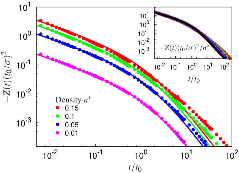
Figure 1: Dimensionless negative VACF $-Z(t)$ for the dilute planar Lorentz gas for Brownian dynamics. Symbols correspond to simulation results, full lines to the first-order density approximation. Density increases from bottom to top. Inset: Rescaling of $-Z(t)$ over $n^{*}$

The simulations for Brownian tracer particles in the low-density range include 5 trajectories for each of the 155 different obstacle realizations drawn for each density, except for $n^{*}=0.01$ where 500 different obstacle realizations where examined. We measure time in terms of microscopic scale $t_{0}:=\sigma^{2}/D_{0}$, i.e., the time needed for the particle to diffuse one obstacle radius without obstruction. The algorithmic time $\tau_{B}$ should be much smaller than $t_{0}$ and here we used $\tau_{B}=0.0025t_{0}$. The negative velocity autocorrelation function $-Z(t)$ is displayed in Fig. 1 on double-logarithmic scales covering four non-trivial decades in time and more than three orders of magnitude in signal. For the smallest density $n^{*}=0.01$ the data coincide with the theoretical first-order density approximation for all times. The time axis in the figure starts at $t=\tau_{B}$ and the small increase in the first data points visible is still affected by the algorithmic resolution. The curves corresponding to moderate densities still follow the first-order low-density prediction at short times but start to deviate at long times. The long-time decay is slower than the expected one quantified by an apparent exponent which becomes smaller upon increasing the obstacle density. The crossover regime shows only a slight flattening of the curvature consistent with the observed increase of the exponent. The inset in Fig. 1 corroborates very nicely the direct density dependence of the VACF following from Eq. (48). All simulation results overlap in the rectification with the theoretical curve besides the exponent variations discussed above. Let us mention that for the ballistic case a numerical confirmation of the long-time tail with universal exponent has been achieved only recently [30], yet the amplitude for the power law still deviated by 25% from the theoretical value for $n^{*}=0.005$. Furthermore our simulation for a Brownian walker allows to compare the VACF for all times to the theory since the VACF is known beyond its asymptotic behavior.

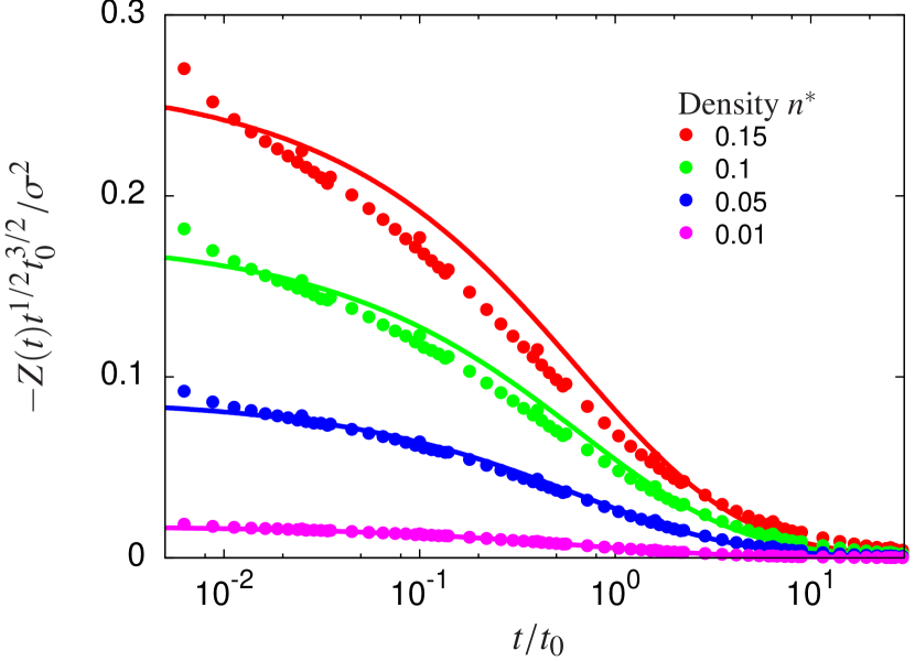
Figure 2: Negative VACF $-Z(t)$ rectified by the short-time prediction $(t/t_{0})^{-1/2}$. Symbols correspond to our simulation results, full lines to the first-order-density approximation. Density increases from bottom to top.

For a more thorough examination of the short-time behavior (Fig. 2) it is advantageous to rectify the VACF with respect to the predicted $t^{-1/2}$ behavior of Eq. (53). For the smallest density again a perfect agreement is observed. The moderate densities are still well described by the first-order-density theory reflecting the fact that the particle did not have time to undergo collisions with more than one obstacle. At short times the effects arising from a finite $\tau_{B}$ amplify as the system becomes denser, because the number of collisions per $\tau_{B}$ is augmented by up to a factor of 15. For the highest density $n=0.15$ we measure already 0.026 collisions on average between the algorithmic assignment of new random velocities. Assuming a Poissonian distribution for the scattering events the probability that two collisions take place in this time interval is roughly about $0.1\%$ and therefore not completely negligible.

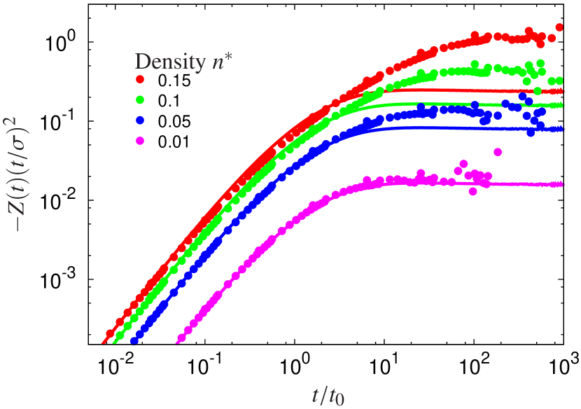
Figure 3: Long-time behavior of $Z(t)$ rectified by the long-time tail $(t/t_{0})^{-2}$. Symbols correspond to the simulation results, full lines are the first-order-density approximation. Density increases from bottom to top.

A rectification plot for the long-time behavior is depicted in Fig. 3. The VACF reaches the predicted scaling $t^{-2}$ for all densities, yet the observed plateau values at long times increase stronger than expected. For the ballistic Lorentz gas it has been shown that such an increase arises due to a competition of the long-time tails and the critical relaxation at the percolation transition [30]. There, the underlying fractal structure induces anomalous transport for the mean-square displacement [48] resulting in a fractal power-law decay of the VACF. The dynamics of the two-dimensional Brownian motion close to the percolation transition shall be discussed elsewhere [49].

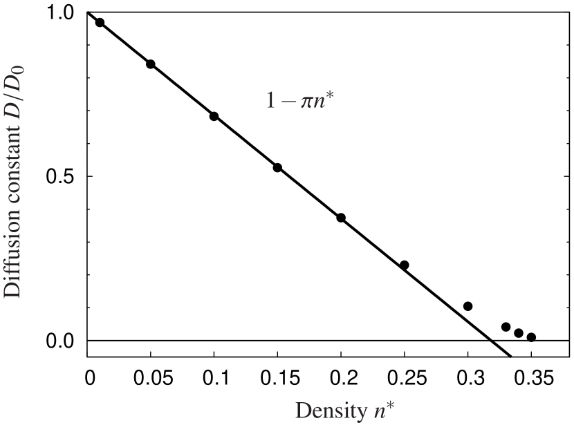
Figure 4: Long-time diffusion coefficient $D$ as a function of reduced obstacle density $n^{*}=n\sigma^{2}$. Symbols correspond the simulation results, the straight line $D/D_{0}=1-\pi n^{*}$ is the first-order-density approximation.

The long-time diffusion coefficients were extracted via $D=\lim_{t\to\infty}(1/4)\mathrm{d}\delta r^{2}(t)/\mathrm{d}t$ from the simulated mean-square displacements. The suppression of the long-time diffusion coefficient predicted in Eq. (49) is shown in Fig. 4. Up to densities of about $n^{*}=0.2$ the data follow quite nicely the predictions; above, higher order corrections gain importance. Nevertheless the first-order theory provides a remarkably good description of the data for all densities. Extrapolation suggests that the diffusion coefficient should vanish at $n^{*}=1/\pi=0.318..$ which is surprisingly close to the measured critical density of the percolation transition $n_{c}^{*}=0.359..$ [49].

8 Conclusion and Outlook

The notion that correlations quickly die out at time scales beyond some characteristic relaxation time of the problem has been shown to be incorrect in general. Besides the meanwhile established long-time anomalies due to momentum conservation in fluids [14, 15], a second paradigm leading to persistent correlations is identified. Quenched disorder implies repeated encounters with the same obstacle, and the information encoded in the exclusion of the configuration space manifests itself in measurable quantities such as the mean-square displacement or the velocity autocorrelation function.

Previous studies focused on the ballistic motion in quenched disorder [20, 21] where the theoretical analysis is quite involved, and the long-time anomalies could be considered as merely a peculiarity of the Lorentz model. The identification of similar persistent correlations for hopping transport in disordered lattices [31, 32, 33] suggests that memory effects may apply to a much larger class of systems. Here we have calculated the memory effects for a Brownian particle in a random environment of hard scatterers to first order in the obstacle density. We conclude that the only ingredient necessary for the long-time tails is the frozen disorder. Since disorder is ubiquitous in nature and the effects arise at all obstacle densities, we conclude that the power laws in the VACF are present for all real systems.

We have confirmed our analytical results by computer simulation for Brownian motion in a disordered array of obstacles. The Brownian particle follows the first-order theory quantitatively at low densities and qualitatively for moderate ones confirming that the long-time anomaly persists for all densities where diffusion occurs in the long-time limit. Furthermore, we have shown that the first-order-density expansion gives a reliable picture for Brownian dynamics, in contrast to the ballistic case.

The Brownian dynamics in the presence of hard obstacles displays a second power law in the VACF at short times which is due to single scattering events from an obstacle. These effects have no analog in the ballistic case nor in hopping transport in disordered lattices.

In the present study the unobstructed dynamics is considered to be a random walk where momentum does not play a role. For a colloidal particle suspended in a fluid and moving through a dilute course of obstacles, one may expect that both the vortex diffusion of momentum in the fluid as well as the repeated encounters with static obstacles leads to an algebraic long-time decay of the VACF. Since the decay $t^{-d/2}$ due to vortex diffusion for unconfined motion is slower than the one for the obstructed motion $t^{-(d+2)/2}$ one may anticipate that momentum conservation is more important than steric hindrance at least for long times. Yet, the obstacles can also carry away momentum and the vortex diffusion in the fluid should be cut off at time scales where the agitated fluid encounters an obstacle. For the case of a wall in three dimensions it has been shown that the long-time anomalies are suppressed [17, 18, 19] to $t^{-5/2}$ rather than $t^{-3/2}$. Hence, for a disordered system in a fluid a competition between both scenarios appears to be relevant, yet no theory is available. Computer simulations for dense hard sphere liquids have indicated a crossover from a positive tail due to vortex diffusion as well as a negative tail in the densely packed regime, where the cages act as a quasi-frozen disordered environment [50]. This phenomenology has been recently corroborated for Lennard-Jones particles [51].

Hydrodynamic fluctuations in two-dimensional fluids lead to a series of divergences in the correlation functions. The diffusion coefficient in an infinite system is expected to be (logarithmically) divergent since the fluid cannot carry momentum away fast enough. For a dilute density of static obstacles one may hope that some of these effects are regularized in a natural way, giving an intriguing interplay of non-analytic behaviors; a theory for such a scenario, however, remains an open question.

9 Acknowledgments

Financial support from the Deutsche Forschungsgemeinschaft via contract No. FR 850/6-1 is gratefully acknowledged. This project is supported by the German Excellence Initiative via the program “Nanosystems Initiative Munich (NIM).”

References

- [1] A. Einstein, On the motion of small particles suspended in liquids at rest required by the molecular-kinetic theory of heat, Ann. Phys. 17 (1905) 549–560.
- [2] M. von Smoluchowski, Zur kinetischen theorie der brownschen molekularbewegung und der suspensionen, Ann. Phys. 326 (14) (1906) 756–780.
- [3] P. Hänggi, F. Marchesoni, Introduction: 100 years of Brownian motion, Chaos 15 (2005) 026101.
- [4] P. Hänggi, H. Thomas, Stochastic processes: Time evolution, symmetries and linear response, Phys. Rep. 88 (4) (1982) 207 – 319.
- [5] E. Frey, K. Kroy, Brownian motion: a paradigm of soft matter and biological physics, Ann. Phys. (Leipzig) 14 (1-3) (2005) 20–50.
- [6] L. Gammaitoni, P. Hänggi, P. Jung, F. Marchesoni, Stochastic resonance, Rev. Mod. Phys. 70 (1) (1998) 223–287.
- [7] P. Hänggi, F. Marchesoni, Artificial brownian motors: Controlling transport on the nanoscale, Rev. Mod. Phys. 81 (1) (2009) 387–442.
- [8] P. Reimann, P. Hänggi, Introduction to the physics of Brownian motors, Appl. Phys. A 75 (2) (2002) 169–178.
- [9] R. D. Astumian, P. Hänggi, Brownian motors, PHYSICS TODAY 55 (11) (2002) 33–39.
- [10] P. Hänggi, G. L. Ingold, Fundamental aspects of quantum Brownian motion, CHAOS 15 (2).
- [11] J. Dunkel, P. Hänggi, Relativistic Brownian motion, Phys. Rep. 471 (1) (2009) 1 – 73.
- [12] J. B. Perrin, Mouvement brownien et réalité moléculaire, Ann. Chim. Phys. 19 (5565) (1909) 5–114.
- [13] P. Langevin, Sur la theéorie de movement brownien, C. R. Hebd. Seances Acad. Sci. 146 (1908) 530–533.
- [14] B. J. Alder, T. E. Wainwright, Velocity autocorrelations for hard spheres, Phys. Rev. Lett. 18 (23) (1967) 988–990.
- [15] B. J. Alder, T. E. Wainwright, Decay of the velocity autocorrelation function, Phys. Rev. A 1 (1970) 18.
- [16] B. Lukić, S. Jeney, C. Tischer, A. J. Kulik, L. Forró, E.-L. Florin, Direct observation of nondiffusive motion of a Brownian particle, Phys. Rev. Lett. 95 (16) (2005) 160601.
- [17] B. Felderhof, Effect of the wall on the velocity autocorrelation function and long-time tail of Brownian motion, Journal of Physical Chemistry B 109 (45) (2005) 21406–21412.
- [18] S. Jeney, B. Lukic, J. A. Kraus, T. Franosch, L. Forro, Anisotropic memory effects in confined colloidal diffusion, Phys. Rev. Lett. 100 (24) (2008) 240604.
- [19] T. Franosch, S. Jeney, Persistent correlation of constrained colloidal motion, Phys. Rev. E 79 (3) (2009) 031402.
- [20] A. Weijland, J. M. J. van Leeuwen, Non-analytic density behaviour of the diffusion coefficient of a Lorentz gas II, Physica (Amsterdam) 38 (1968) 35.
- [21] M. H. Ernst, A. Weijland, Long time behaviour of the velocity auto-correlation function in a Lorentz gas, Phys. Lett. A 34 (1971) 39.
- [22] H. van Beijeren, Transport properties of stochastic Lorentz models, Rev. Mod. Phys. 54 (1) (1982) 195–234.
- [23] C. Bruin, Logarithmic terms in the diffusion coefficient for the Lorentz gas, Phys. Rev. Lett. 29 (25) (1972) 1670–1674.
- [24] C. Bruin, A computer experiment on diffusion in the Lorentz gas, Physica 72 (1974) 261.
- [25] B. J. Alder, W. E. Alley, Long-time correlation effects on displacement distributions, J. Stat. Phys. 19 (1978) 341.
- [26] B. J. Alder, W. E. Alley, Decay of correlations in the Lorentz gas, Physica A 121 (3) (1983) 523–530.
- [27] C. P. Lowe, A. J. Masters, The long-time behaviour of the velocity autocorrelation function in a Lorentz gas, Physica A 195 (1-2) (1993) 149–162.
- [28] W. Götze, E. Leutheusser, S. Yip, Dynamical theory of diffusion and localization in a random, static field, Phys. Rev. A 23 (1981) 2634.
- [29] W. Götze, E. Leutheusser, S. Yip, Correlation functions of the hard-sphere Lorentz model, Phys. Rev. A 24 (1981) 1008.
- [30] F. Höfling, T. Franosch, Crossover in the slow decay of dynamic correlations in the Lorentz model, Phys. Rev. Lett. 98 (14) (2007) 140601.
- [31] T. M. Nieuwenhuizen, P. F. J. van Velthoven, M. H. Ernst, Density expansion of transport properties on 2D site-disordered lattices: I. General theory, J. Phys. A: Math. Gen. 20 (12) (1987) 4001–4015.
- [32] M. H. Ernst, T. M. Nieuwenhuizen, P. F. J. van Velthoven, Density expansion of transport coefficients on a 2d site-disordered lattice. ii, Journal of Physics A: Mathematical and General 20 (15) (1987) 5335–5350.
- [33] D. Frenkel, Velocity auto-correlation functions in a 2d lattice Lorentz gas: Comparison of theory and computer simulation, Phys. Lett. A 121 (8-9) (1987) 385–389.
- [34] R. Balian, From Microphysics to Macrophysics, 2nd Edition, Vol. II, Springer, Berlin, 2007.
- [35] J. A. Dix, A. Verkman, Crowding effects on diffusion in solutions and cells, Ann. Rev. Biophys. 37 (1) (2008) 247–263.
- [36] M. R. Horton, F. Höfling, J. O. Rädler, T. Franosch, Anomalous diffusion develops among crowding proteins bound to a supported lipid bilayer, Soft Matter doi:10.1039/b924149c, arXiv:1003.3748.
- [37] B. J. Sung, A. Yethiraj, Lateral diffusion and percolation in membranes, Phys. Rev. Lett. 96 (22) (2006) 228103.
- [38] B. J. Sung, A. Yethiraj, Lateral diffusion of proteins in the plasma membrane: Spatial tessellation and percolation theory, J. Phys. Chem. B 112 (1) (2008) 143–149.
- [39] J. J. Sakurai, Modern Quantum Mechanics, 2nd Edition, Prentice Hall, 1993.
- [40] B. J. Ackerson, L. Fleishman, Correlations for dilute hard core suspensions, J. Chem. Phys. 76 (5) (1982) 2675–2679.
- [41] B. U. Felderhof, R. B. Jones, Cluster expansion of the diffusion kernel of a suspension of interacting Brownian particles, Physica A 121 (1-2) (1983) 329 – 344.
- [42] B. U. Felderhof, R. B. Jones, Diffusion in hard sphere suspensions, Physica A 122 (1-2) (1983) 89 – 104.
- [43] R. B. Jones, Memory function moment analysis of dynamic light scattering data, J. Phys. A: Math. Gen. 17 (1984) 2305–2317.
- [44] I. A. Stegun, M. Abramowitz (Eds.), Handbook of Mathematical Functions, Dover, New York, 1965.
- [45] J. P. Boon, S. Yip, Molecular Hydrodynamics, Dover Publications, Inc., New York, 1991, reprint.
- [46] A. Scala, T. Voigtmann, C. De Michele, Event-driven Brownian dynamics for hard spheres, J. Chem. Phys. 126 (13) (2007) 134109.
- [47] F. Höfling, T. Munk, E. Frey, T. Franosch, Critical dynamics of ballistic and Brownian particles in a heterogeneous environment, J. Chem. Phys. 128 (16) (2008) 164517.
- [48] F. Höfling, T. Franosch, E. Frey, Localization transition of the three-dimensional Lorentz model and continuum percolation, Phys. Rev. Lett. 96 (2006) 165901.
- [49] T. Bauer, F. Höfling, T. Munk, E. Frey, T. Franosch, Localization transition in the two-dimensional Lorentz model, arXiv:1003.2918 [cond-mat.soft].
- [50] S. R. Williams, G. Bryant, I. K. Snook, W. van Megen, Velocity autocorrelation functions of hard-sphere fluids: Long-time tails upon undercooling, Phys. Rev. Lett. 96 (8) (2006) 087801.
- [51] P. H. Colberg, F. Höfling, Accelerating glassy dynamics on graphics processing units, arXiv:0912.3824 [physics.comp-ph] (2009).