Extraction of neutron observables from inclusive lepton scattering on nuclei

Abstract

We analyze new JLAB data for inclusive electron scattering on various targets. Computed and measured total inclusive cross sections in the range $0.3\lesssim x\lesssim 0.95$ show on a logarithmic scale reasonable agreement for all targets. However, closer inspection of the Quasi-Elastic components bares serious discrepancies. EMC ratios with conceivably smaller systematic errors fare the same. As a consequence the new data do not enable the extraction of the magnetic form factor (FF) $G_{M}^{n}$ and the Structure Function (SFs) $F_{2}^{n}$ of the neutron, although the application of exactly the same analysis to older data had been successful. We incorporate in the above analysis older CLAS collaboration data on $F_{2}^{D}$. Removing some scattered points from those, it appears possible to obtain the requested neutron information. We compare our results with others from alternative sources. Special attention is paid to the $A=3$ iso-doublet cross sections and EMC ratios. Present data exist only for ³He, but the available input in combination with charge symmetry enables computations for ³H. Their average is the computed iso-scalar part and is compared with the empirical modification of ³He EMC ratios towards a fictitious $A=3$ iso-singlet.

I Introduction.

Nearly a decade has passed since the publication of JLab experiment E89-008, describing inclusive scattering of electrons on various targets nicu1 ; arrd . Those extended older SLAC data on the D and He isotopes rock and later ones

for beam energies $E\leq 3.6$ GeV on D, ⁴He and several medium and heavy targets ne3 . A similar experiment in 1999 used $E$=4.05 GeV electrons arr89 .

In the JLab experiments E03-102, E02-90, $5.76$ GeV unpolarized electrons were scattered over angles $\theta=18^{\circ},22^{\circ},26^{\circ},32^{\circ},40^{\circ}$ and $50^{\circ}$. Total inclusive cross sections covering wide kinematics, have been measured for targets D, ^3,4He, ⁹Be, C, Al, Cu. Out of this extensive data bank, only the EMC ratios $\mu^{{}^{3,4}He},\mu^{Be}$ and $\mu^{C}$ for one scattering angle $\theta=40^{\circ}$ and limited kinematics have been published until this day seely . In addition cross section data over the entire measured kinematic range and for all targets have been made available ag . We also mention data taken with a $E=5.0$ GeV beam, the analysis of which has not yet been completed ps .

In order to define notation, we start with the total cross section per nucleon for inclusive scattering of unpolarized electrons, reduced by the Mott cross section $\sigma_{M}$. For given beam energy $E$, scattering angle $\theta$ and energy loss $\nu$ one has

$$K^{A}(x,Q^{2},\theta) = \frac{d^{2}\sigma^{A}(E;\theta,\nu)}{d\Omega\,d\nu}\Big{/}\sigma_{M}(E;\theta,\nu)$$

$$= \frac{2xM}{Q^{2}}F_{2}^{A}(x,Q^{2})+\frac{2}{M}F_{1}^{A}(x,Q^{2}){\rm tan}^{2}(\theta/2),$$

$F_{1,2}^{A}(x,Q^{2})$ above are nuclear SFs, which depend on the squared 4-momentum transfer $q^{2}=-Q^{2}=-({|\mbox{\boldmath$q$}|}^{2}-\nu^{2})$ and the Bjorken variable $0\leq x=Q^{2}/2M\nu\leq M_{A}/M\approx A$ with $M$, the nucleon mass.

Several approaches have been proposed for an analysis of inclusive cross sections in the PWIA, or the same with some FSI distortions benh ; oset . We report below on an analysis, based on a previously tested non-perturbative GRS approach asr1 ; gr . Our application covers the entire corpus of new data (ND) also beyond the restricted targets and kinematics of the published material, reported in Refs. seely ; ag . To those we add an analysis of D CLAS data osipd . Except for the treatment of the $A=3$ targets, the method of analysis for the new data is identical to the one, previously applied to the older data (OD). We therefore shall not detail steps, but mention References instead.

We adhere in the following to a generalized convolution, linking $F_{k}^{A}$ and $F_{k}^{p,n}$ (see for instance Ref. asr1 )

$$F^{A}_{k}(x,Q^{2}) = \int_{x}^{A}\frac{dz}{z^{2-k}}\bigg{[}f_{p}^{A}(z,Q^{2})ZF_{k}^{p}\bigg{(}\frac{x}{z},Q^{2}\bigg{)}+f_{n}^{A}(z,Q^{2})NF_{k}^{n}\bigg{(}\frac{x}{z},Q^{2}\bigg{)}\bigg{]}\bigg{/}A.$$ (2)

$$\approx \int_{x}^{A}\frac{dz}{z^{2-k}}f^{A}(z,Q^{2})\bigg{[}ZF_{k}^{p}\bigg{(}\frac{x}{z},Q^{2}\bigg{)}+NF_{k}^{n}\bigg{(}\frac{x}{z},Q^{2}\bigg{)}\bigg{]}/A.$$ (3)

Above $f^{A}$ are SFs for a fictitious nucleus composed of point-particles which cannot be excited, irrespective of the value of $Q^{2}$ aku . Alternatively one interprets $f$ as a kind of generalized distribution function of the centers of interacting nucleons in a target.

The functions $f^{A}$ for finite $Q^{2}$ can only be calculated exactly for the lightest nuclei and have otherwise to be modeled asr1 . In the PWIA the above norm can be shown to be 1. The same is expected for any bona-fide distribution function. We shall return to this point in detail.

In virtually all previous applications one did not distinguish between distribution functions $f_{p,n}^{A}$, which are different for $p$ and $n$. However, in a treatment of the lightest odd nuclei, their difference may matter and a proper treatment ought to use Eq. (1.2).

Eqs. (1.2), (1.3) feature nucleon SFs $F_{k}^{p,n}$, which in general are off their mass shell. However, in the region of our main $Q^{2}\gtrsim(2.5-3.0)$ GeV², those effects may be neglected, and the same holds for the mixing of nucleon SFs in the proper expression for $F_{2}^{A}$ atw ; sss . Since the data do not reach the deepest inelastic range $x\lesssim 0.2$, screening effects may also be disregarded kul . For $Q^{2}\lesssim 3.0$ GeV², for which (pseudo-)resonance structure is not yet extinguished, we shall use $F_{2}^{p}$ from Ref. chr1 , while for larger $Q^{2}$ we rely on a parametrization of the resonance-averaged $F_{2}^{p}$ arneo . References to $F_{2}^{n}$ can be found in asr1 .

It is convenient to decompose nucleon SFs $F_{k}^{N}$ in Eq. (1.2) into parts, describing the absorption of a virtual photon, either exciting the absorbing $N$ into hadrons (partons) or not ($\gamma^{*}+N\to N$). The amplitudes for the latter vanish except for $x=1$, in which case those may be expressed as standard combinations of electro-magnetic FFs. A similar division applies to nuclear SFs. Denoting by $[{\tilde{G}}^{N}]^{2}=[Z(G^{p})^{2}+N(G^{n})^{2}]/A\,\,$, the $Z,N$ weighted average of the squared nucleon FFs, one finds from Eq. (3) their nuclear analogs ($\eta=Q^{2}/(4M^{2})$)

$$F_{1}^{A,NE}(x,Q^{2}) = \frac{f^{PN,A}(x,Q^{2})}{2}[{\tilde{G}}_{M}^{N}(Q^{2})]^{2}]\,$$ (4)

$$F_{2}^{A,NE}(x,Q^{2}) = xf^{PN,A}(x,Q^{2})\frac{[{\tilde{G}}_{E}^{N}(Q^{2})]^{2}+\eta[{\tilde{G}}_{M}^{N}(Q^{2})]^{2}}{1+\eta}$$ (5)

Nuclear inelastic processes (NI) dominate in general, but occasionally one needs to include the above quasi-elastic parts (NE).

In inclusive spectra one distinguishes the following kinematic regions :

a) Deepest Inelastic Scattering for $x\lesssim 0.2$, with characteristic (anti-) screening effects.

b) NI-dominated Deep Inelastic Scattering (DIS) region, $0.2\lesssim x\lesssim x_{r}(Q^{2})$ with $x_{r}(Q^{2})\approx\bigg{[}(M_{R}^{2}-M^{2})/Q^{2}+1\bigg{]}^{-1}$, the Bjorken $x$ for resonance excitation.

c) NI-NE interference region for $x_{r}(Q^{2})\lesssim x\lesssim 0.85-0.95$.

d) Quasi-Elastic (QE) region around the Quasi Elastic Peak (QEP), $0.95\lesssim x\lesssim 1.05$, dominated by NE, and only weakly perturbed by NI tails, provided $Q^{2}\lesssim(4-5)$ GeV².

e) ’Deep Quasi-Elastic’ (DQE) region, $x\gtrsim 1.05$, dominated by NE. Cross sections there are very small in comparison with those in regions a)-d) and again, are for not too high $Q^{2}$, only weakly perturbed by inelastic tails.

In the following all measured total cross sections, whether published as EMC ratios of the above in a limited kinematic range, or as yet unpublished results for the entire measured kinematic ranges seely ; ag , shall be referred to as ’data’.

This note is organized as follows. We first report in Section IIa on general features of total inclusive cross sections, which we illustrate by a few samples for iso-singlet targets. From a comparison of experimental and computed total cross sections over the larger part of the kinematic $x$ range $0.35\lesssim x\lesssim 0.95$, we conclude that in the DIS region NI components are apparently reliably computed.

For increasing $x$ towards the QE region, NE components grow, start to compete with NI, and for not too large $Q^{2}$, finally overtake those. We show that around the QEP and in both wings, theory and data for NE applied to ND almost never agree.

Particular attention is paid to the $A=$3 iso-doublet, where we distinguish between $p,n$ as struck nucleons (Section IIB). Section IIC deals with EMC ratios derived from the material in Sections IIA,B. Since in the only publication thus far, the prime interest is a sample of EMC ratios for the lightest nuclei in the classical EMC region $x_{min}^{data}\lesssim x\lesssim 0.9$, a comparison with computed results, including for ³He, is limited to those.

In Section III we focus on the QE region and try to extract the reduced magnetic FF $\alpha_{n}=G_{M}^{n}/[\mu_{n}G_{d}]$ ($G_{d}$). We apply a previously formulated criterion, which has to be fulfilled before one can attempt an extraction. For ND data it appears virtually never fulfilled.

As an alternative source we include in Section III the CLAS data for $F_{2}^{D}$ osipd . Removing in the QE region a few manifestly scattered data points, the above-mentioned criterion is satisfactorily met by the CLAS data, which we endowed with $(2-3)\%$ systematic errors. We shall show that the extracted averaged reduced neutron magnetic FF $\alpha_{n}$ agree with the OD results.

In Section IV we exploit the same CL data in order to extract the neutron SF $\,F_{2}^{n}$ along lines used in the past rtf2n . In the concluding Section we discuss both theoretical and experimental aspects of the extraction of $n$ properties from inclusive cross sections.

II Cross sections and derived observables.

II.1 Total inclusive cross sections.

Total inclusive cross sections are usually computed from forms like Eq. (3), with $f^{A}(x,Q^{2})$ in some approximation, for instance the PWIA (or DWIA), or on the light cone. Below we adhere to a non-perturbative GRS theory, which we have exploited over years asr1 ; gr . Obviously, starting from one given Hamiltonian, different approaches evaluated to sufficiently high order in suitable expansion coefficients, should ultimately tend to the same final results rj . Our choice of the GRS approach is only motivated by, in general, better convergence of low order terms.

We start with an outline of the derivation for $f_{p}=f_{n}$, referring for details to Refs. asr1 ; gr and vkr . In Eq. (2.8) of the latter reference we mentioned and discussed the GRS expansion

$$\phi(q,y_{G})=\sum_{n}\bigg{[}\frac{M}{q}\bigg{]}^{n}\phi_{n}(y_{G})$$ (6)

of a related function $\phi(q,y_{G})$ of $q=|\vec{q}|$, the 3-momentum along the $z$-axis, and of a relativistic generalization of the non-relativistic West scaling variable gur $\,\,(\eta=Q^{2}/4M^{2}$)

$$y_{G} = y_{G}^{\infty}\bigg{(}1-\frac{1-x}{2(A-1)(1+x^{2}/\eta)}\bigg{)}$$

$$y_{G}^{\infty} = \frac{M}{\bigg{(}1+x^{2}/\eta\bigg{)}^{1/2}}(1-x)$$

$y_{G}^{\infty}$ is that variable for an infinitely heavy recoiling spectator. In the following we retain only the two lowest order terms in the GRS series (6) (we abbreviate $y_{G}$ by $y$).

$$\phi^{A;GRS}(q,y)\approx\phi^{A;(0)}(q,y)+(M/q)\phi^{A;(1)}(q,y)$$ (7)

The lowest order term is expressed by means of the single-hole spectral function (Spft) $S(E,k)$ of the target (Ref. vkr , Eq. (2.9)) and the second term describes the dominant FSI.

The appearance of Spfts in expressions for the lowest order SF is common to all approaches. Those are mainly distinguished by the definition or choice of the 4th component of the missing 4-momentum. For instance in the GRS theory the latter is determined by the requirement, that the ejected $N$ and the spectator shall, to equal measure, be off their mass-shells gur . Its contribution $\tilde{\phi^{(0)}}$ is detailed in Ref. gr , Eqs. (66),(67).

The next order GRS term for the usually dominant FSI reads (cf. Ref. vkr , Eq. (2.17a))

$$(M/q)\phi^{A;(1)}(y,q)=(M/q)\int_{0}^{\infty}\frac{ds}{2\pi}e^{isy}\int\int d{\vec{r}}_{1}d{\vec{r}}_{2}\rho_{2}^{A}({\vec{r}}_{1},{\vec{r}}_{2};{\vec{r}}_{1}^{\prime},{\vec{r}}_{2})[i{\tilde{\chi}}^{A}_{q}({\vec{b}},z;s)],$$ (8)

contains two components. The first is a two-particle density matrix $\rho_{2}$, not diagonal in one coordinate, which in principle may be obtained from the product of two $A$-particle ground state wave functions, integrating out $A-2$ coordinates. For $A>4$ one usually makes a short-cut, using an interpolating approximation asr1

$$\rho_{2}^{A}({\vec{r}}_{1},{\vec{r}}_{2};{\vec{r}}_{1}^{\prime},{\vec{r}}_{2}))\approx\rho_{1}^{A}(r_{1})\rho_{1}^{A}(r_{2})\bigg{[}\frac{\rho_{1}^{A}(r_{1},r_{1}^{\prime})}{\rho_{1}^{A}(r_{1})}\bigg{]}\sqrt{g^{A}(|{\vec{r}}_{1}-{\vec{r}}_{2}|)g^{A}(|{\vec{r}}_{1}^{\prime}-{\vec{r}}_{2}|)},$$ (9)

where $\rho_{1}^{A}(1,1)=\rho_{1}^{A}(1)$ and $g^{A}$ are the single-particle density and the pair-distribution function. Using the Negele-Vautherin Ansatz nv , the non-diagonal single-particle density $\rho_{1}^{A}{\vec{r}}_{1},{\vec{r}}_{1}^{\prime})$ is computed from

$$Y^{A}(s) \equiv \frac{\rho_{1}^{A}({\vec{r}}_{1},{\vec{r}}_{1}^{\prime})}{\rho_{1}^{A}(r_{1})}$$

$$\approx\int\frac{d^{3}k}{(2\pi)^{3}}e^{i{\vec{k}}{\vec{s}}}\,\,n^{A}(k) = \frac{1}{2\pi^{2}s}\int_{0}^{\infty}dk\,k\,{\rm sin}(ks)n^{A}(k)$$ (10)

$n^{A}(k)$ is the single particle momentum distribution, obtained by integrating the Spft over the missing energy $E$

$$n^{A}(k)=\int_{0}^{\infty}dES^{A}(k,E)$$ (11)

The second factor in the integrand in (2.3) is an off-shell phase factor ${\tilde{\chi}}_{q}({\vec{b}},z;s)$ in terms of the relative coordinates ${\vec{r}}_{1}-{\vec{r}}_{2}=({\vec{b}},z)$; $\,\,{\vec{s}}\equiv{\vec{r}}_{1}-{\vec{r}}_{1}^{\prime}=(\vec{q}/|q|s)$. The appended $q\approx|\vec{p}+\vec{q}|$ is approximately the lab momentum of the nucleon, which absorbed the virtual photon, before a FSI scattering from another $N$ occurs.

In Ref. vkr , Eqs. (2.17b)-(2.21b) we discuss the approximation

$$i{\tilde{\chi}}_{q}(\vec{b},z)\approx\theta(z)\bigg{[}\theta(s-z)-s\delta(s-z)\bigg{]}\Gamma_{q}(b),$$ (12)

with $\Gamma^{(1)}_{q}(b)=-(\sigma_{q}^{tot}/2)(1-i\tau_{q})A_{q}(b)$ the standard on-shell profile function. It is related to the diffractive elastic $NN$ scattering amplitude $f_{q}^{NN}$, with $\tau_{q}={\rm Re}f_{q}/{\rm Im}f_{q}$ and $A_{q}(b)=[Q_{q}(0)]^{2}/4\pi]e^{-[bQ_{q}^{(}0)]^{2}/4}$. With $np$ and $pp$ data of quite different quality, one usually takes an average of the relevant $np$ and $pp$ cross sections asr1 .

Next one transforms the representative terms $\phi(q,y_{G})$ in the GRS expansion (7) by means of a Jacobian

$$J^{A}(x,Q^{2}) = \bigg{|}{\partial y^{A}}/{\partial x}\bigg{|}$$ (13)

$$\approx M\bigg{[}\frac{1+x/\eta}{(1+x^{2}/\eta)^{3/2}}\bigg{]}\bigg{|}1-\frac{(1-x)(2+3x/2\eta-x^{2}/\eta)}{2(A-1)(1+x/\eta)(1+x^{2}/\eta)}\bigg{|}$$

to the distribution function $f^{A}$ in the $x,Q^{2}$ variables

$$\phi^{A}(q,y)\to f^{A}(x,Q^{2}))=J^{A}(x,Q^{2})\phi^{A}\bigg{(}q(x,Q^{2}),y^{A}(x,Q^{2})\bigg{)}$$ (14)

By means of those distribution functions $f^{A}$ one computes the SFs $F_{k}^{A}(x,Q^{2})$ in Eq. (3), and in particular the inelastic parts NI^calc asr1 ; rtv . The elastic components NE are expressed in terms of FFs and the computed distribution functions $f^{A}(z,Q^{2})$ as in Eqs. (4), (5). Their sum defines total cross sections

$$\sigma^{A,tot}={\rm NI}^{calc}+{\rm NE}^{FF}$$ (15)

The above we applied to all E03-102, E02-90 total cross section data.

In view of the fact that only a restricted part of the measured ND data have been published, we first display in Figs. 1a-d, 2a-d a sample of $I$=0 targets, namely D($\theta=18^{\circ},22^{\circ},26^{\circ},32^{\circ}$) and C ($\theta=26^{\circ},32^{\circ},40^{\circ},50^{\circ})$. Those are shown as heavy drawn lines, to be distinguished from heavy dots for data, first shown without error bars.

With exception of remnants of resonance excitations of the lightest nuclei at low $\theta$ (i.e. low $Q^{2}$), the examples of smooth data shown are typical for all targets $A\geq 12$ at similar kinematics.

A cursory glance on the logarithms of the above total cross sections shows reasonable agreement for each scattering angle and target, in particular for the smallest $x$ measured. This holds down to the approach of the resonance region, where NI${}^{calc}\gg$ NE. The read-off agreement thus provides evidence that the calculated NI components in the DIS region are basically correct. In contrast, when moving to the QE and DQE regions, growing discrepancies occur in very small cross sections. In order to understand the nature of the above discrepancies, we separately consider NE and NI components.

In addition to the computed NE^FF, Eqs. (1.4)-(1.5) we define

$$\rm{NE}^{\it extr}=\rm{data}-NI^{\it calc}$$ (16)

Clearly, the semi-empirical NE^extr will show the scatter present in the data, while NE^FF in $\sigma^{A,tot}$, Eq. (15), is a smooth function of $x$, $f^{A}$ and FFs. For perfect data and theory NE from Eqs. (5) and (16) should coincide.

The expression NE^FF in the single photon exchange (SPE), Eq. (5), uses among others $G_{E}^{p}$. Primarily a discrepancy in the ratio $\gamma=\mu_{p}G_{E}^{p}/G_{M}^{p}$, once measured in a Rosenbluth separation, and then by polarization transfer jon . It has led to calculations of two-photon exchange (TPE) corrections on an isolated $p$ blun ; amt ). Those have been shown to reduce the above mentioned discrepancy.

The above TPE have been parameterized in the functional form of a SPE part, which enables the sum SPE+TPE to be considered as an effective SPE amt . All results in the following use that input. Their effect on single bound $p$ appears to change $\sigma^{A}$ for ’bare’ SPE by less than $1\%$. There also exist TPE corrections involving two nucleons, etc., but their contributions have as yet not been determined.

We return to Figs. 1a-d, 2a-d where we display NI^calc (light dots) and NE^FF (light drawn lines), as well as their calculated sum $\sigma^{A,tot}$. Crosses in the above Figs. represent NE^extr, Eq. (16) and those are seen to differ considerably from NE^FF. Missing crosses indicate that NI^calc locally exceeds data.

For growing $x$, NE increasingly competes with NI and eventually dominates, and we thus focus on the QE region. Although on a logarithmic scale a small number of points in the QE regions may occasionally seem to be close to the dotted lines, actual discrepancies come to the fore on linear plots for NE^PP together with NE^extr. The latter now include total error bars, where we added to statistical errors (2-3)$\%$ estimates for systematic ones. Figs. 3a-d are samples for D(18,40), C(18,40). Discrepancies appear to grow with both $A$ and $Q^{2}$ and are occasionally quite erratic. Clearly the ND cross sections and the results of standard computations are at odds.

This is not the case for the analysis of the OD data, where we applied the same code. We illustrate this by a comparison with Figs. 4a,b,c for $\sigma^{D}(E=4.045$ GeV;$\,\theta=15^{\circ},30^{\circ},55^{\circ})$, taken from Ref. rtv . The logarithmic scale and Bjorken value on the vertical and horizontal scales, as well as symbols and curves correspond to those in the above Figs. 1,2. We added dashed curves for empirical inelastic NI parts, which cause NE${}^{PP}\approx{\rm NE}^{extr}$. In the critical region between the QEP and the (first) resonance, NI^emp exceeds NI^comp by less than 15$\%$. It is obvious that in the QE region OD data and computed results agree far better than is the case for the ND. We shall return to this issue in the Discussion.

II.2 The $A$=3 iso-doublet.

Amongst the ND are also the first results for ³He after the old SLAC data rock . Those are of particular interest, since ³He is the lightest stable odd nucleus with a large relative nucleon excess. Approximate charge symmetry invites a simultaneous study of ³He and ³H, although for the latter there are as yet no data.

We thus separately treat $N=p,n$ and start with the lowest order term $\phi^{A;(0)}$, given in I, Eq. (2.9) (or equivalently Eqs. (66), (67) in Ref. gr ). This clearly demands knowledge of Spfts $S^{A=3}_{N}$ for the ejected nucleon $N=p,n$. In those one distinguishes between a 2-body continuum and a D spectator state. The latter occurs only if $I_{3}^{A=3}=I_{3}^{N}$ for the 3-components of the iso-spins.

Using $\psi^{A=2}_{n}$ for spectator states with separation energy ${\cal E}_{n}^{A=2}$, one writes for the Spft and momentum distribution $n^{A=3}(k)=\int_{E_{min}}dE,\,\ S^{A=3}(k,E)$ of a $A=3$ nucleus

$$S^{I_{3}^{A=3}}(k,E) = \sum_{j\neq D}|\langle\Psi_{0}^{I_{3}^{A=3}}|\Psi_{j\neq D}^{I_{3}^{A=2}}*\vec{k};I_{3}^{N}\rangle|^{2}\delta(E-{\cal E}^{A=2}_{j\neq D})$$ (17)

$$+ \delta(I_{3}^{A=3},I_{3}^{N})|\langle\Psi_{0}^{I_{3}^{A=3}}|\Psi^{D}*\vec{k};I_{3}^{N}\rangle|^{2}\delta(E+B_{D})$$

$$n^{I_{3}^{A=3}}(k) = \sum_{j\neq D}|\langle\Psi_{0}^{I_{3}^{A=3}}|\Psi_{j\neq D}^{I_{3}^{A=2}}*\vec{k};I_{3}^{N}\rangle|^{2}+\delta(I_{3}^{A=3},I_{3}^{N})|\langle\Psi_{0}^{I_{3}^{A=3}}|\Psi^{D}*\vec{k};I_{3}^{N}\rangle|^{2},$$ (18)

with $B_{D}$ the binding energy of the D. One then derives the corresponding lowest order $A=3$ distribution functions ($\beta=M\nu/q;\,\,\xi=E/M+x-1$)

$$f_{N}^{I_{3}^{A=3};(0)}(x,Q^{2})=\frac{J^{(3)}(x,Q^{2})}{4\pi^{2}}\bigg{[}\theta(x-1)\int_{0}^{\infty}dE\int_{\beta\xi}^{\infty}dkkS_{N}^{I_{3}^{A=3}}(k,E)+\theta(1-x)$$ (19)

$$* \bigg{(}\int_{M(1-x)}^{\infty}dE\int_{\beta\xi}^{\infty}dkkS_{N}^{I_{3}^{A=3}}(k,E)+\int_{0}^{M(1-x)}dE\int_{-\beta\xi}^{\infty}dkkS_{N}^{I_{3}^{A=3}}(k,E)\bigg{)}\bigg{]}$$

$$+ \delta(I_{3}^{A=3},I_{3}^{N})\int_{|y|}^{\infty}dkkn^{A=3}_{N;D}(k),$$

with $y={\rm lim}_{E\to-B_{D}}\,\,(\beta\xi)$. $J^{(3)}(x,Q^{2})$ above is the Jacobian, Eq. (13) and

$$n_{N;D}^{A=3}(k)=\int_{0}^{\infty}dES_{N}^{I_{3}^{A=3}}(k,E)\delta(E+B_{D}),$$ (20)

the D-component of the $A=3$ momentum distribution.

Regarding the dominant FSI term, Eq. (2.3), one distinguishes as before between a nucleon ’1’ being a $p$ or a $n$, etc. In the evaluation the following assumptions shall be made:

i) $p,n$ number densities $\rho_{1}$ deV are equal in either ³He or ³H, but not in both species.

ii) As to single $p,n$ momentum distributions, we computed $n_{p,n}^{{}^{3}{He}}(k)$ from the generalization Eq. (18) of (9) and found small differences for single $p$ and $n$ components.

iii) In the generalization of Eq. (9) we assume $g^{nn}(|{\vec{r}}_{1}-{\vec{r}}_{2}|)=g^{pp}(|{\vec{r}}_{1}-{\vec{r}}_{2}|)$ and $g^{pn}(|{\vec{r}}_{1}-{\vec{r}}_{2}|)=g^{np}(|{\vec{r}}_{1}-{\vec{r}}_{2}|)$, which change Eq. (8) into

$$\rho_{2}^{I_{3}^{A=3}}(1,2;1^{\prime}2)\to$$ (21)

$$1/3 \bigg{[}\rho_{2}({\vec{r}}_{1,p},{\vec{r}}_{2,p};{\vec{r}}^{\prime}_{1;p},{\vec{r}}_{2,p})+\rho_{2}({\vec{r}}_{1,p},{\vec{r}}_{2,n};{\vec{r}}^{\prime}_{1,p},{\vec{r}}_{2,n})+\rho_{2}({\vec{r}}_{1,n},{\vec{r}}_{2,p};{\vec{r}}^{\prime}_{1,n},{\vec{r}}_{2,p})\bigg{]}_{I_{3}^{A=3}}$$

$$\approx 1/3\bigg{[}Y(s)\rho_{1}({\vec{r}}_{1})\rho_{1}({\vec{r}}_{2})\bigg{]}_{I_{3}^{A=3}}\bigg{[}2\sqrt{g_{pn}(r)g_{pn}(|{\vec{r}}-{\vec{s}}|)}+\sqrt{g_{pp}(r)g^{pp}(|{\vec{r}}-{\vec{s}}|)}\bigg{]}$$

The functions $g_{pp}$ and $g_{pn}$ have been taken from Ref. sss . Neglecting the small differences in the single $N$ momentum distributions $n_{N}^{I_{3}^{A=3}}$, the points i)-iii) leave no $N$ dependence: $\phi^{A;(1)}$ depends only on $I_{3}^{A=3}$.

Next we replace ${\vec{r}}_{1},{\vec{r}}_{2}$ by relative and CMS coordinates ${\vec{r}},{\vec{R}}$ and perform the $R$-integration in (8)

$$T({\vec{b}},z)=\int d^{3}R\rho_{1}(|{\vec{R}}+{\vec{r}/2}|)\rho_{1}(|{\vec{R}}-{\vec{r}}/2|),$$ (22)

which leaves one angular and one radial integration in the expression for ${\tilde{\phi}}^{(1)}$. Consequently, $Y$ in Eq. (21) appears as a factor in

$$\int d{\vec{R}}\rho_{2}^{A}(1,2;1^{\prime},2)\to\frac{1}{3}Y^{A}(s)T^{A}(b,z){\cal G}({\vec{b}},z;s),$$ (23)

with ${\cal G}$ a combination of pair-distribution functions in (21).

Finally, using approximation (2.7) for the phase, the FSI contribution (2.3) becomes

$$\phi^{A=3;(1)}(q,y) = \frac{1}{3}{\cal R}e\int_{0}^{\infty}ds{\rm e}^{isy}Y(s)\int_{0}^{\infty}dbb$$ (24)

$$\bigg{[}\int_{0}^{s}dz\bigg{(}T(b,z){\cal G}(b,z;s)\bigg{)}-sT(b,s){\cal G}(b,s;s)\bigg{]},$$

where 6-dimensional integrals in Eq. (8) are reduced to 2-dimensional ones. Again, Eq. (2.6) in Ref. vkr produces the corresponding $f^{A=3;(1)}(x,Q^{2})$. We checked that $f^{FSI;(1)}\ll f^{(0)}$, but did retain the FSI term $f^{(1)}$ in all calculations.

We now reach the crucial input, which is the outcome of extensive calculations for various Spfts $S^{{{}^{3}He}}$, performed by the Rome-Pisa group gianni . Those employed the following $NN$ interactions:

a) purely 2-body $NN$ forces (B2; AV18 wir ), neglecting $V_{coul}$.

b) the same as a), including $V_{coul}$.

c) the same as b) with an additional 3$N$ force (B2+B3; AV18 UR9 pud ).

The list above does not refer to ³H. All items were intended as input for ³He calculations but clearly, only b) and c) are realistic options with different sophistication. In contrast, option a) lacks $V_{coul}$ between protons. i.e. the most obvious and dominant charge-symmetry breaking part and is therefore not suited for ³H3 calculation.

However in the absence of other parts, the missing $V_{coul}$ turns the hamiltonian for a) to the the charge-symmetric one corresponding to b), i.e. for ³H.

However, option a) is for a ³He Hamiltonian which lacks Coulomb forces between the protons. Thus disregarding additional charge-symmetry breaking effect, option a) describes the iso-partner ³H. In particular for the basic distribution functions one has the following relations for the iso-partners

$$f_{n}^{{{}^{3}}H}=f_{p}^{{{}^{3}}He(no\,\,coul)};f_{p}^{{{}^{3}}H}=f_{n}^{{{}^{3}}He(no\,\,coul)}$$ (25)

Using Eq. (3) one has for the SFs

$$F_{2}^{{{}^{3}}He}(x,Q^{2})=\int_{x}^{3}dz\frac{1}{3}\bigg{[}2f_{p}^{{{}^{3}}He}(z,Q^{2})F_{2}^{p}\bigg{(}\frac{x}{z},Q^{2}\bigg{)}+f_{n}^{{{}^{3}}He}(z,Q^{2})F_{2}^{n}\bigg{(}\frac{x}{z},Q^{2}\bigg{)}\bigg{]}$$ (26)

and either form

$$F_{2}^{{{}^{3}}H}(x,Q^{2})=\int_{x}^{3}dz\frac{1}{3}\bigg{[}f_{p}^{{{}^{3}}H}(z,Q^{2})F_{2}^{p}\bigg{(}\frac{x}{z},Q^{2}\bigg{)}+2f_{n}^{{{}^{3}}H}(z,Q^{2})F_{2}^{n}\bigg{(}\frac{x}{z},Q^{2}\bigg{)}\bigg{]}$$ (27)

$$= \int_{x}^{3}dz\frac{1}{3}\bigg{[}f_{n}^{{{}^{3}}He(no\,\,coul)}(z,Q^{2})F_{2}^{p}\bigg{(}\frac{x}{z},Q^{2}\bigg{)}+2f_{p}^{{{}^{3}}He(no\,\,coul)}(z,Q^{2})F_{2}^{n}\bigg{(}\frac{x}{z},Q^{2}\bigg{)}\bigg{]}$$ (28)

Next we compare the above considerations with some results. Figs. 5a,b show for $Q^{2}=2.5$, respectively 7.5 GeV² the distribution functions $f_{p,n}^{{{}^{3}}He}(x,Q^{2})$, Eq. (13). The drawn, dashed and dotted correspond to interactions B2(0), B2(0+1), B2+B3(0+1), where the numbers indicate the order of terms retained. Since FSI terms are retained, results for B2(0) only serve to indicate the relative importance of the two terms. Fig. 5c compares $f_{p}^{A=3,I_{3}}(x,Q^{2}=5)$, Eq. (25). to which we shall return in Section IIC.

At this point we need and mention, that for any $Q^{2}$ the norm of the lowest order term ${\cal N}_{x}=\int_{0}^{3}dxf_{p,n}^{A=3;(0)}(x,Q^{2})=1$. A more extensive discussion can be found in the Appendix.

The above $A=3$ distribution functions follow a standard pattern for all light $A$ rtvemc : for increasing $Q^{2}$ the peak of $f^{A=3}$ increases and the width shrinks correspondingly. For instance, for $Q^{2}$ increasing from 2.5 to 10.0 GeV², the B2 $p$ peaks increase from 4.041 to 5.394 and for $n$ from 3.483 to 4.648. Peak values for B2+B3 are $\approx 4\%$ lower than for B2 and are correspondingly wider. Next, for the same $Q^{2}$ those are intermediate between the same for D and ⁴He.

Fig. 6 displays computed SFs $F_{2}^{{{}^{3}}He}$ for fixed $\theta=40^{\circ}$ and variable $Q^{2}(x,\theta)$, using Eqs. (26) with B2 or B2+B3 interactions. The results for those are practically indistinguishable and quite close to the extracted SF, using data and $R\approx 0.36/Q^{2}$ for the ratio of inclusive scattering of virtual longitudinal and transverse photons. The lower curve in Fig. 6 is for $F_{2}^{{{}^{3}}H}$, Eq, (28): with no data, there is no extracted parallel. One notices however, the seizable difference in predictions for the members of the iso-doublet.

Figs. 7a,b present on a linear scale data and computed inclusive cross sections on ³He for $\theta=18^{\circ},40^{\circ}$. Cross sections for $\theta=40^{\circ}$ for ³He, using either B2 or B2+B3 interactions are in good agreement with data. This outcome should be compared with the same for other targets shown in Figs. 1 on a log scale, and the same for the QE range in Figs. 2 on a linear scale. The rather poor fit for ³He, $\theta=18^{\circ}$ is in striking contrast with the same for $\theta=40^{\circ}$, in spite of the use of the same underlying analysis. We cannot forward any theoretical explanation.

II.3 EMC ratios.

At least some difficulties in understanding ND total cross section data may be due to unknown systematic errors, the size of which can only be estimated. Since the D is amongst the targets, part of those errors may cancel in EMC ratios $\mu^{A}=F_{2}^{A}/F_{2}^{D}$. For that reason alone is it of interest to compare measured with computed ratios.

The new EMC data are for a few discrete $\theta$ and thus not for fixed $Q^{2}$. Although the resulting $Q^{2}$ dependence is mild, it should be borne in mind that, for instance, for the chosen angle $\theta=40^{\circ}$, data on the released, or measured additional $x$-ranges, cover $2.80\lesssim Q^{2}{\rm(GeV}^{2})\lesssim 6.12$, which is not an insignificant variation in $\mu(Q^{2})$. The published data are for $x_{min}^{data}\leq x\lesssim 0.9$, $x_{min}^{data}\approx 0.35$ seely , and correspond to what occasionally is called the ’classical’ EMC range. Within that range the variation of $Q^{2}$ has less spread and causes less than $1\%$ variations in EMC ratios.

Measured $\mu^{{}^{4}He}$ and $\mu^{{}^{12}C}$ seely have a somewhat smaller slope than older data, in particular for ⁴He (see for instance Ref. kp . In Figs. 8a,b we compare the new data with previously computed GRS results for $Q^{2}=3.5,5.0$ GeV² rtvemc and for additional $Q^{2}$, close to the above-mentioned binned ones. The agreement is reasonable.

We also mention a prediction, based on the $Q^{2}$-independence of $F_{2}^{p,D}(x\approx 0.20,Q^{2})$ arneo . Since all distribution functions $f^{A}$ are negligible for $x\lesssim 0.4$, one may replace the lower integration limit in the expression (2.1) for $F_{2}^{A}$ by 0. Then using unitarity, i.e. ${\cal N}[f^{A}]\approx{\cal N}[f^{A;(0)}]=1$, all $F_{2}^{A}(x\approx 0.20,Q^{2})$ computed by Eq. (3) are predicted to be roughly independent of $Q^{2}$ as well as of $A$. Consequently EMC ratios $\mu^{A}(x,Q^{2})$ ought to intercept the $x$-axis at a value $\mu^{A}(x\approx 0.2,Q^{2})\approx 1$ rtvemc . The above holds when only one distribution function is involved, i.e. for $I=0$ nuclei, or when an averaged $f^{A}$ is sufficiently accurate in all other cases.

The actual crossover $\mu^{A,D}=1$ for most nuclei and for several $\mu^{A,A^{\prime}}$) is $x_{co}\approx(0.2-0.3)$, whereas the intercept of the $I=0$ ND data, seems to occur for somewhat higher $x\approx 0.33$ seely .

Again we separately discuss the case of the $A=3$ iso-doublet with different $f_{p}$ and $f_{n}$. In the previous Section we presented results for computed SFs and cross sections for the $A=3$ doublet, using various input options. For completeness we add for ³He the ’standard’ extraction of its SF from cross section data. Although the above exists for several options, we report only on computed results for B2+B3 interactions and calculated EMC ratios as $F_{2}^{A}/F_{2}^{D}$, respectively $\sigma^{A}/\sigma^{D}$.

As discussed above we need option a) in Section IIB for ³He with no $V_{coul}$, in order to compute the the SF for iso-partner ³H. Data are much desired petra pace , but it will take years before those will become available and can be confronted with calculated $F_{k}^{{}^{3}{H}}$, like from Eq. (28) (cf. also sss , pace , afnan ).

In Fig. 9a we show 3 curves for $\mu^{A=3;F_{2}}(\theta=40^{\circ})$ from ratios of SFs. The upper and lower ones are for ³He and ³H, while the middle one for half their sum, is the computed $I=0$ part of either member of the iso-doublet. One notices the widely different behavior of the two ratios: In the classical EMC region $\mu^{{}^{3}{He}}>1,$ has a positive $x$-slope and shows no minimum for medium $x$. In contrast $\mu^{{}^{3}{H}}<1$, has a negative $x$-slope and an unexpectedly deep minimum for $x\approx 0.7$. The iso-singlet part has positive slope, crosses 1 at $x\approx 0.8$ and has no visible minimum.

Fig. 9b shows $\mu^{A=3;\sigma}(\theta=40^{\circ})$, but now as ratios of cross sections, which are seen to differ from the one in Fig. 9a: $\mu^{{}^{3}He}\gtrsim 1$ for $x\lesssim 0.85$ and has a maximum for $x\approx 0.75$. In contrast $\mu^{{}^{3}H}<1$, has negative $x$-slope and shows a shallow minimum for $x\approx(0.6-0.7)$. Essentially the same holds for the iso-scalar part, but the ³He part there pushes the $I=0$ part an amount $\approx 0.1$ upwards on the $\mu$-scale.

The empty circles in Fig. 9b are the data of Seely $et\,al.$ for ³He from ratios of bona fide cross sections, yet are called by the authors ’raw data’ (empty circles in Fig. 9b). Comparison with the upper drawn curve shows rough agreement. In contrast to a genuine calculation of the iso-scalar part (dashed curve), the above-mentioned authors modify the above ’raw data’ in a standard fashion, which does not require information on ³H. This leads to a fictitious $I=0$ nucleus with $N=Z=A/2$ amounting to

$$f_{p,n}^{A(Z,N)}\approx f^{A}(Z=N)\approx f^{A}\bigg{(}\frac{A}{2},\frac{A}{2}\bigg{)}$$ (29)

The above is considered to be a model for the EMC ratio of an even nucleus with $I\neq 0$ and instructive, even for interpolation to $A=3$ seely .

The above results hardly change when $\theta$ runs over the entire measured range, and this holds in particular for their $I_{3}$ dependence. One should keep in mind that the anyhow small EMC effect is the deviation from 1 of the ratio of small numbers. That effect even diminishes when going to the lightest nuclei, increasing its precarious sensitivity. In this relation we recall the $I$-spin dependence in Fig. 5c of the $p$-distribution function in the iso-doublet, assuming iso-spin symmetry after correcting for $V_{coul}$. The two may well be related.

III The magnetic FF of the neutron and CLAS data.

In the previous sections we encountered clear discrepancies between the NE component in the ND and OD results in the QE regions of total inclusive cross sections. Their description requires the dominant reduced $n$ magnetic FF $\alpha_{n}=G_{n}^{M}/[\mu_{n}G_{D}]$ in the QE region. In the following we recall attempts to isolate and to extract $\alpha_{n}$.

At this point we remark that on the one hand the entities $G_{M}^{n}$ (and $F_{k}^{n}$ considered in the following section) are needed to determine the total SFs $F_{A}$ and the inclusive (reduced) cross sections $\sigma^{A}$. On the other hand one wishes to extract those from QE data. The procedure is to use some starting values in the input, compare the output until self-consistency is reached and the outcome compared with the staring values.

The expressions (4), (5) locate two functions with pronounced peaks for $x\approx 1$. Those are the NE part of the reduced cross section $K^{A:NE}(x,Q^{2};E,x)$, Eqs. (1.1), (2.11), and the linking distribution function $f^{A}(x,Q^{2})$, functions of 5, respectively 3 variables.

In appears that their ratio $K^{A;NE}/f^{A}$ is primarily a function of $Q^{2}$ with only weak additional dependence on $x,\theta,E$ and $A$. As suggested in the past we turn the above into a criterion, to be fulfilled by candidates $x_{l}$ for extraction

For sufficiently accurate and smooth data one tries to locate a $continuous$ $x$-range in the QE region, for which the above ratio does not vary, by more than a prescribed amount, say, 10$\%$. If available, one finds (cf. Eq. (4.3) in Ref. rtv )

$$\alpha_{n}|\mu_{n}|=\bigg{[}\frac{2MK^{A,NE}/[vfG_{d}]-B^{2}/\eta}{1+{\rm tan}^{2}(\theta/2)/v}-\bigg{(}\alpha_{p}\mu_{p}\bigg{)}^{2}\bigg{]}^{1/2},$$ (30)

where $Q^{2}$-dependence is implicit. Above $G_{d}$ is the standard dipole FF, $v=x^{2}/2(1+\eta)$, $\beta_{N}=G_{E}^{N}/G_{d}\,\,\,\alpha_{N}=G_{M}^{N}/[\mu_{N}G_{d}]$ and $B^{2}=\beta_{p}^{2}+\beta_{n}^{2}$. Eq. (30) generalizes for $f_{n}\neq f_{p}$ as

$$\frac{N}{A}f_{n}[\alpha_{n}\mu_{n}]^{2}+\frac{Z}{A}f_{p}[\alpha_{p}\mu_{p}]^{2}=\frac{MK^{A;NE}/vG_{d}^{2}-\bigg{(}Zf_{p}\beta_{p}^{2}/(A\eta)+Nf_{n}\beta_{n}^{2}\bigg{)}}{1+{\rm tan}^{2}(\theta/2)/v},$$ (31)

$\alpha_{n}(Q^{2})$ is of course only a function of $Q^{2}$, but due to imperfect data and theory the algorithm produces an inherent, weak dependence on the chosen points $x$. Whereas there is no physical meaning to individual $x$-dependent results, it is natural to define the extracted $\alpha_{n}(Q^{2})=\equiv\langle\alpha_{n}(Q^{2})\rangle=\langle\alpha_{n}(x;Q^{2})\rangle_{x}$ as an appropriate average over the selected $x-$range. For all previously investigated OD data the above criterion is met for a suitable number of continuous $x$-points (see Table in Ref. rtv ). As to ND, only for D$(\theta\lesssim 32^{\circ})$ could we find 2-3 such points. However, those points appear to produce through Eq. (30) a value for $\alpha_{n}$, far from the OD results for similar $Q^{2}$.

Like the material discussed in Sections I, II, also the above indicates that in the QE region the ND and OD data sets do not match. We emphasize two points, relevant for OD. One is the very applicability of the suggested analysis for OD data, in contrast to the same for ND. Moreover $different$ sets with approximately the same $Q^{2}$, produce essentially the same $\alpha_{n}(Q^{2})$, providing evidence for internal consistency rtv .

As a last resource we invoke the CLAS collaboration data on $F_{2}^{D}$, which have not been subjected to a similar analysis before. Those are available for a dense net of $Q^{2}$ ($\Delta Q^{2}$ = 0.05 GeV²), which for each $Q^{2}$ cover a wide and dense $x$-range ($\Delta x$ =0.009) osipd . We apply the above mentioned criterion regarding the $K/f$ ratio to those data and look for continuous $x$ ranges around the QEP for $\theta=18^{\circ},22^{\circ},26^{\circ},32^{\circ}$, which approximately correspond to $Q^{2}\approx 2.50,3.275,4.175,5.175$ GeV². Regrettably CL data do not extend to larger $Q^{2}$, covering $\theta=40^{\circ},50^{\circ}$ in ND.

Also for CL one cannot, strictly speaking, apply the above criterion for a continuous $x$-range in every data set. However, a representative number of candidate $x$-points remains after removal of at most 1 or 2 points per set, for which the observed scatter of neighboring points exceeds 10$\%$. The extracted $\langle\alpha_{n}(Q^{2})\rangle$ appears to match the OD results.

We first show in Figs. 10a,b in much the same way as in Figs. 1-2, the components NI^D,calc, NE^D,FF and NE^D,extr for two of the above four data sets with $Q^{2}$= 3.275, 4.175 GeV². Whereas clearly useful around the QEP, some disagreement between the two NE representations grows towards the inelastic wing of the QE peak. It is similar in size and shape as for OD data rtv , but not anywhere as disastrous as for the above-mentioned ND.

In Table I we entered $F_{2}^{D}$ for the above four angles over a range of $x$ and correspondingly varying $Q^{2}$ values. In the last 3 columns we compare: i) the values $extracted$ from the ND data, assuming the standard transverse/longitudinal ratio $R\approx 0.36/Q^{2}$; ii) the same $computed$ from Eq. (3); iii) the CL data for $F_{2}^{D}$. Differences seem largest around the QEP and occasionally switch sign. No similarly large abberations are apparent in the analysis of linear plots of the OD data.

Table II contains the reduced magnetic FF $\alpha_{n}^{CL}$ from the CLAS data, $Q^{2}$, the range and number of chosen $x$-points. Column 4 states the averaged $\langle\alpha_{n}(Q^{2})\rangle$ with the error of the mean. To the statistical errors we included guessed 2$\%$ systematic ones, added in quadrature.

In Fig. 11 we assemble $\alpha_{n}(Q^{2})$ as extracted from the OD and CL data for 4 values $Q^{2}$= 2.501, 3.275, 4.175, 5.175 GeV², together with a previously extracted parametrization, Eq. (5.4), Ref. rtv . For completeness we added to the above all $\alpha_{n}$ with $Q^{2}\geq 2.5$ GeV² rtv , extracted from OD data. The CL and OD data sets produce essentially the same results and trend.

The above figure displays $\langle\alpha_{n}(Q^{2})\rangle$, extracted from CL for closely spaced $Q^{2}$ around the 4 values above. While the former vary by $(0.5-1.0)\%$, going from one to a neighboring $Q^{2}$-bin, entries within each bin show larger variations within a standard deviation of $\langle\alpha_{n}(Q^{2})\rangle$.

In the same figure we entered $\alpha_{n}(Q^{2})$, recently extracted from the cross section ratio $D(e,e^{\prime}n)p/D(e,e^{\prime}p)n$ for $Q^{2}=(1.0-4.8)$ GeV². Each FF point has been measured with a less than 3$\%$ error, but again, for $Q^{2}\gtrsim 2.5$ GeV², and most outspoken for $Q^{2}\gtrsim$ 3.4 GeV², the scatter between adjacent points, is often far larger. The results (Fig. 5 in Ref. brooks ) have also been included in Fig. 11 together with those of Ref. lung .

We conclude this section, mentioning a recent calculation of space and time-like nucleon FFs using a light-front framework melo . Whereas space-like $p$ FFs are well reproduced, the computed $\alpha_{n}$ show a maximum, then diminishes and tends to 0 for large $Q^{2}$. That result disagrees considerably with those displayed in Fig. 11, where practically coinciding extractions from the CLAS collaboration data and the OD, produce a continuous decrease, which persists out to $Q^{2}\approx 10\,$GeV².

IV Extraction of $F_{2}^{n}$ from CLAS data.

The neutron SF $F_{2}^{n}$ complements information from $F_{2}^{p}$ on the valence quark distribution functions $u_{v},d_{v}$ in the $N$: its knowledge is a minimal requirement to disentangle the two distributions. Lacking reliable information on $F_{2}^{n}$, one occasionally invoked the SU(6) result $[F_{2}^{n}/F_{2}^{p}]_{SU6}=3/5$ which amounts to $u_{v}=2d_{v}$. Alternatively, one uses the ’primitive’ choice $F_{2}^{n}=2F_{2}^{D}-F_{2}^{p}$, the reliability of which is restricted to $x\lesssim 0.35$.

It is clearly desirable to have empirical information on $F_{2}^{n}$ along with $F_{2}^{p,D}$ for $x\gtrsim 0.3$ in order to determine $N$ parton distributions. With no free $n$ target available, one has to extract $F_{2}^{n}$ from bound neutrons. The preferred target has been the D, for which the nuclear information is simplest and most accurately known, but the literature also describes the extraction of $F_{2}^{n}$ from future precision data on the SFs for ³He,³H (e.g. Refs. pace ; sss ; afnan ) and heavier targets rtf2n .

Several extraction methods have in the past been proposed. For instance, an approximate inversion of Eq. (3) requires reliable data points on $F_{2}^{A}$, and preferably for several targets. Previously we had found that data were barely sufficient to extract $F_{2}^{n}$ from a single binned ${\bar{Q}}^{2}=(3.5-4.0)$ GeV². We summarize the steps of the followed procedure rtf2n , which will also be exploited below:

i) Assume $C(x,Q^{2})\equiv F_{k}^{n}(x,Q^{2})/F_{k}^{p}(x,Q^{2})$ to be independent of $k$.

ii) $C(0)=1$, as implied by a finite Gottfried sum $\int_{0}^{1}dx[F_{2}^{p}(x,Q)2-F_{2}^{n}(x,Q^{2})]/x$.

iii) The validity for $x\lesssim 0.30-0.35$ of the ’primitive’ approximation $F_{2}^{D}=[F_{2}^{p}+F_{2}^{n}]/2$, $i.e.$ $C=2F_{2}^{D}/F_{2}^{p}-1$. In practice we use $p,D$ data for 2 points, chosen to be $x=0.15,0.25$. The information ii), iii) mainly determines the decrease of $C(x,Q^{2})$ from 1 for $x$, increasing from 0 to about $x\lesssim 0.6$.

iv) A last step is a chosen parametrization for $C(x,Q^{2})=\sum_{k\geq 0}d_{k}(Q^{2})(1-x)^{k}$. For $k=3\,\,$, ii)-iii) leave one parameter to be determined and the natural candidate is $C(1,Q^{2})=d_{0}(Q^{2})=1-\sum_{k\geq 1}d_{k}(Q^{2})$.

A remark on $C(1)$ is in order here. Both SFs $F_{2}^{p,n}(x,Q^{2})$ vanish for finite $Q^{2}$ beyond the lowest inelastic pion production threshold at $x_{\pi\,thr}(Q^{2})\approx 1/\big{[}2M\mu_{\pi}/{Q^{2}}+1\big{]}$, and the NI continuum is therefore isolated from the elastic peak at $x=1.$ The SFs of the latter are given by Eqs. ($\ref{a3a}),(\ref{a3b}$) in terms of FFs. Neglecting $G_{E}^{n}$, one finds (typos in Ref. rtf2n have been corrected below)

$$\lim_{x\to 1}C^{FF}(x,Q^{2})=\Big{[}\frac{\mu_{n}\alpha_{n}(Q^{2})}{\mu_{p}\alpha_{p}(Q^{2})}\Big{]}^{2}\Big{[}1+\frac{4M^{2}}{Q^{2}}\Big{(}\frac{\gamma(Q^{2})}{\mu_{p}}\Big{)}^{2}\Big{]}^{-1}$$ (32)

with

$$\gamma(Q^{2}) = \frac{\mu_{p}G_{E}^{p}(Q^{2})}{G_{M}^{p}(Q^{2})}$$

$$\frac{\alpha_{n}(Q^{2})}{\alpha_{p}(Q^{2})} = \frac{G_{M}^{n}(Q^{2})/\mu_{n}}{G_{M}^{p}(Q^{2})/\mu_{p}}$$ (33)

$C$ has then been determined by a least square fit for the sum $\sum_{x_{m}}^{x_{M}}$ and not point-by-point in $x$. Naturally, any parametrization of $C$, and in particular iv) above, ascribes values to $C$ in the un-physical region $1\gtrsim x\gtrsim x_{r}(Q^{2})$.

The extracted parameter $d_{0}(Q^{2})=C(1,Q^{2})$ fairly rapidly reaches a plateau for increasing $Q^{2}$. Since $\lim_{x\to 1}F_{2}^{p,n;NI}(x,Q^{2})=0$, it is not surprising to find that values for $C(x\lesssim 1,Q^{2})$ on the plateau, i.e. the extrapolation from the adjacent non-physical region to the largest $x>x_{thr}$ and ultimately to $x=1$, depend sensitively on the upper limit taken in the $x$-sum above. Thus for $x_{M}$=0.75 and increasing $Q^{2},4\lesssim Q^{2}(\rm GeV^{2})\lesssim 10$, the extracted $C(1,Q^{2})$ decreases from 0.38 to 0.27, while $C^{FF}(1,Q^{2})$, Eq. (5), barely decreases form 0.38 to 0.37. For a slightly larger $x_{M}=0.80$, $C(1,Q^{2})$ decreases from 0.34 to 0.25 over a much narrower $Q^{2}$-interval than for $x_{M}=0.75$.

The procedure has been checked by a re-calculation of $F_{2}^{D}$, using the extracted $F_{2}^{n}$ in Eq. (3): the initial $F_{2}^{D}$ appears accurately reproduced. Figs. 12a,b show $C^{D}(x,Q^{2})$ as well as $F_{2}^{p,n}$ for $Q^{2}=2.5,7.5$ GeV², $x_{M}=0.75$. Although influencing $C$ for $x$=1, one can only barely distinguish between $C(x\lesssim 0.85,Q^{2})$, computed for either $x_{M}=0.75$ or 0.80.

Alternative attempts have been made in the past in order to obtain $F_{2}^{n}$, all of which use a D target. One for instance replaces the distribution function $f^{PN,D}$ in Eq. (3) by a momentum distribution or some generalization of the latter, and uses it to ”smear” nucleon SFs MT . From he difference $\langle F_{2}^{n}\rangle_{f}=F_{2}^{D}-\langle F_{2}^{p}\rangle_{f}$, featuring folded or ’smeared’ SFs, the ”bare” $F_{2}^{n}$ has to be de-convoluted. An iteration method has recently been tested on the MAID parametrization for $F_{2}^{N}$ kmk . The reported success may in part be due to the fact that the procedure, as well as the parameterized input, imply the use of a smooth average. Application to real data with non-negligible may well run into the above discussed difficulties. We also mention an extraction of $F_{2}^{n}$ from essentially the Impulse Approximation for $f^{PN,D}$, using the parameterized ratio $F_{2}^{D}/F_{2}^{p}$, $F_{2}^{p}$ and the D wave function achl . Most published $C(x,Q^{2})$ follow the same trend for $x\lesssim 0.75$ and are primarily distinguished by the extrapolated $C(x=1)$.

Finally we recall the extraction of the leading twist moments of $F_{2}^{p,D}$ from the CL data. By means of a convolution such as is Eq. (3), those are subsequently used to construct parallel twist moments for $n$ osip3 . Also the above analysis uses some averaging, which may in part underly its feasibility. No inversion leading to $F_{2}^{n}(x,Q^{2})$ has been attempted there.

V Discussion and Conclusions.

It has been our goal to describe the Jlab experiments E103-102, E02-90 on inclusive electron scattering from various targets, specifically for total cross sections and EMC ratios seely . Subsequently we tried to extract from those the (reduced) magnetic FF $\alpha_{n}(Q^{2})$ and the SF $F_{2}^{n}(x,Q^{2})$ of a neutron bound in a nucleus. Those are respectively, the dominant part of the NE component in the QE region and a vital component of the inelastic part of the total cross section.

Also for the ND, we used the GRS approach which has previously been applied to all older experimental information rtv . Only minor changes in theoretical elements have been applied since, for instance the inclusion of two-photon exchange corrections to the electric FF of the proton.

We first mention that the most reliable results from the OD data have been obtained in the DIS region, where inclusive scattering is entirely inelastic. For the smallest $x$ we found agreement with data, not rarely to within (2-3)$\%$. For increasing $x$, strongly decreasing NI parts have to be accurately known in order to isolate with precision the NE parts, dominating the QE region rtv . For medium $x$ between the ”elastic tails” of (pseudo-)resonances and their peaks disagreements appear, which are reflected in the difference between the extracted and computed NE components.

A possible cause of the above disagreements could be uncertainties in the proton SF. We checked that a mild relative change of NI, which grows to $\approx 15\%$ in the NE/NI interference region, and again decreases towards the higher NI resonances, brings about agreement. Such an uncertainty in the parametrization of the of $F_{2}^{p}$ in the required $Q^{2}$ region, apparently hardly affects the quality of the extracted $F_{2}^{p}$ chr1 .

Next we considered the extraction of the $n$ magnetic FF from data in the QE region. We utilized a previously formulated criterion for such an extraction, which requires a continuous set of eligible $x$-points, for which the ratio of the $x$-dependent reduced total cross section and the computed distribution function falls within pre-determined limits. The criterion could be fulfilled for all old data sets, which moreover showed consistency: The same $\alpha_{n}$ resulted from different data sets with overlapping $Q^{2}$ values.

From the above new precision data one expects agreement of at least the same quality. Using exactly the same program as before we analyzed all measured data, of which only a fraction has been published. The major results are as follows:

a) Even in the DIS region, the best agreement is not better than (5-6)$\%$, and not infrequently of both signs.

b) Measured EMC ratios for light iso-scalar nuclei approximately agree with previous data and calculations .

c) The same seems to hold for model-independent features for $x\approx 0.20$

d) It is virtually impossible to satisfy in any QE region our criterion on candidate $x$-points for the extraction of $\alpha_{n}$. As a rule NE parts, as the difference of and computed NI components, do not anywhere match NE, computed from FFs. The required changesin NI leading to a match, by far exceed the moderate ones described in Ref. rtv .

At this point we mention a suggestion to integrate the QE peak over some $x$-interval and to extract $\alpha_{n}$ from those arrpc . We doubt whether the suggested procedure can produce reliable averages for locally varying relative systematic errors.

The only alternative material which we could use in the above analysis, are the CLAS collaboration data on D osipd , which have apparently not been analyzed before. From those we could extract both $\alpha_{n}$ and $F_{2}^{n}$ and the former essentially matched older results.

Particular attention has been paid to the $A=3$ iso-doublet. Many years after the first data were taken, the new experiments contain information on ³He, while also theory has much advanced. Most significantly there are now available results of exact calculations of the $A=3$ single $p,n$ Spectral Functions for several $NN$ interactions. Those underly the calculation of the dominant contribution of the separate $p,n$ distribution functions in both ³He and ³H, with the latter using charge symmetry when $V_{coul}$ is neglected. We thus calculated for the GRS theory the SFs of ³He and ³H and inclusive cross sections.

We start with $\sigma^{{{}^{3}}He}$ for all 6 measured angles and found only crude agreement for the lower angles, and (very) good correspondence for the largest ones, in particular for $\theta=40^{\circ}$. Using one and the same theory for all, theory cannot be blamed for the striking dissimilarity.

Next we computed the two EMC ratios $\mu^{A=3}(\theta=40^{\circ})$ and their iso-scalar mean, once as ratios of $F_{2}$ and then alternatively from cross sections. The data for ³He in the classical EMC region hover around 1 and do not show a minimum around $x\approx 0.5-0.6$. About the same is predicted by theory.

The latter is quite different for ³H, for which theory predicts a more standard behavior with $\mu\lesssim$ 1 and a shallow minimum. Lack of data prevent a comparison with the above outcome. However, one may discuss the computed iso-scalar part, which resembles a standard EMC ratio with a growing negative slope for decreasing $A$ from $A=12$, down to D. The slope of the iso-vector part $\mu^{A=3;I=0}(\theta=40^{\circ})$ lies in between the same for ⁴He and the D.

As to ’raw data’, in a standard procedure one estimates $\mu^{A}$ for nuclei with a nucleon excess, replacing that EMC ratio by one for a fictitious isobar with $Z=N=A/2$. The published data for the iso-scalar part of ³He about agree with the computed ones. It should be clear that theory computes a real result, while the above data relate to a somewhat dubious extrapolation to the lowest $I\neq 0$ nucleus.

We return to the enigmatic outcome for several non-isolated ND data. Since the same tools were used before, the most extreme conclusion could be incompatibility of the old and new sets. A milder judgement blames systematic errors. We had included those as a fixed estimated percentage, but it is clear from the scatter of neighboring accurate points, that more than average systematic errors are required in order to bring about agreement.

We also wish to recall that all cross section data sets are reported to have normalization uncertainties running from (2.2-2.7)$\%$ ag . Those may in part cause some of the observed discrepancies, but for instance not the discrepancies between inclusive cross sections on ³He for $\theta=18^{\circ}$ and $40^{\circ}$ in similar data sets.

A question of different nature is, whether a fundamental parton description may significantly modify results based on a used hadronic representation. Only recently has attention been re-drawn to two old communications regarding a QCD treatment of nuclear SFs in the single gluon exchange PWIA approximation. That approach leads to a generalized convolution of distribution functions much like Eq. (3), with a simple correspondence between the featuring quantities in the two representations jaffe ; west .

The above approach can actually be extended beyond single gluon exchange, and one shows that at least some higher order QCD corrections can still be accommodated in a convolution rtjw . In fact, formally the same expression (3) holds in both a hadronic and a QCD representation for $F^{A}$, provided one re-interprets $f^{A,PN}$ in the latter as the distribution function of (centers of) nucleons in the target. It is not likely that there are significant QCD contributions which cannot be accommodated in a convolution. At the end of Section II we recalled and actually compared EMC ratios, calculated in the hadron and in a parton representation.

The availability of planned Rosenbluth-separated data naturally simplifies the analysis, but will probably not resolve the exposed problems, as long as the scatter of neighboring points is much larger than the accuracy of each point. For instance $\alpha_{n}$, extracted from Eq. (30) will remain sensitive to the input.

Use of the the same analyzing tools as before, indicates that the new JLab do not confirm previous conclusions, and–related to the above, one cannot extract statistically significant information on the neutron, in contrast to the apparent success, previously obtained from OD. The resolution of this difficulty is clearly highly desired.

VI Acknowledgements.

The authors are grateful to John Arrington, who provided us with all measured total inclusive cross section, being final or not, and made useful remarks. Thanks are equally due to Gianni Salme, who provided the 3 sets of $A=3$ Spectral Functions, which enabled a realistic calculation of SFs for the $A=3$ system.

VII Appendix.

We start with a QCD prediction for the lowest moment $M_{0}(Q^{2})=\int_{0}^{1}dxF_{2}^{p}(x,Q^{2})=0.1471$ of a nuclear SF in the Bjorken limit with $N_{f}=6$ contributing flavors. For any nuclear target a similar moment can be computed, given a parton representation of $F_{2}^{A}$. For several $A$ and finite $Q^{2}=(2.5-10.0)$ GeV², we found values up to 5-6$\%$ lower than for a $p$ rtpart .

We now add the moments of the computed $F_{2}^{{}^{{}^{3}}He}$ to previously reported results for $\langle N\rangle$, D, ⁴He, C, Fe in Table I, rtpart . For low $Q^{2}\approx 2.5$ GeV² the moment of ³He is 16$\%$ higher than for a $p$. That moment rapidly decreases with increasing $Q^{2}$, specifically to 0.1476 for $Q^{2}=10\,$GeV², close to the Bjorken limit. The same for ³H is substantially closer to the previously computed moments of other light and medium-weight targets. As Figs 5. illustrate the above is due to the differences of $f_{p,n}$ and of each distribution function for ³He and ³H. The same causes the differences in the predicted EMC ratios $\mu^{A=3}$.

We return to $f^{A}$ in Eqs. (2.2), (2.3) which we termed the SF of a fictitious nucleus composed of point-nucleus or, alternatively, a distribution function for the centers of nucleons in a nucleus. QCD is clearly not applicable to those artifacts, no matter how high $Q^{2}$ is. Their norm ${\cal N}$, very close to 1, differs from $M_{0}^{A}$ of physical nuclei.

In Section IIB we mentioned that for either choice of $NN$ interaction B2 or B2+B3, the norm of the lowest order part ${\cal N}_{x}(Q^{2})=\int_{0}^{3}dxf_{p,n}^{(0);A=3}(x,Q^{2})$ equals 1 within a few parts per mille: More precisely, for $Q^{2}=(2.5-10.0)$ GeV², ${\cal N}_{x}$ has a minute slope $\approx 0.0024/$GeV². The same holds for ${\cal N}_{y}(q)=\int_{-q/2}^{q_{max}}dy\phi^{(0)}(q,y)$.

The above result for finite $Q^{2}$ is not self-understood. Only in the $Q^{2}\to\infty$ limit can one easily derive ${\cal N}$=1.0. For finite $Q^{2}$ the deviations of the norm from 1 and the minute slope of those deviations as function of $Q^{2}$ are not due to numerical inaccuracies. We note that a total disregard of the missing energy and momentum yields $f(x,Q^{2})=\delta(x-1)$.

It is interesting to observe that the relevant missing energies appear restricted to $-|B_{D}|\lesssim E/M\lesssim 0.012$, which dominates the underlying Spft $S_{p,n}^{A=3}(k,E)$ (negative values occur only for a D-spectator). To a less extreme extent the same holds for the missing momentum: $k/M\lesssim 0.2$. Re-instating finite small missing energies and momenta produces distribution functions with finite $Q^{2}$-dependent widths.

The above emphasizes $A=$3 nuclei, but several points hold for general $A$. For the D a norm 1 is trivial, but a similar observation can, and has been made for ⁴He, for which the underlying Spft is fairly accurately known vkr . For heavier nuclei with models for $\rho_{2}^{A}$ (see Ref. I, Eqs. (9),(10)), the norm ${\cal N}(f)$, when necessary, has been adjusted to 1.

Finally, the above holds for the lowest order part $f^{(0)}$. For the reasons mentioned, it is not evident that, when including FSI contributions, one should apply a small re-normalization correction, due to the relatively small $f^{A=3;(1)}<<f^{A=3;(0)}$. We have not done so in our calculations.

Table 1: Values of $F_{2}^{D}(x,Q^{2})$, extracted and computed from ND, and the same from CL osip3 for a chosen $x$-range (columns 1). Columns 2 give $Q^{2}(x,\theta)$ for that $x$ range and $\theta=18^{\circ},22^{\circ}$, respectively $\theta=32^{\circ},40^{\circ}$. Columns 3,4,5, are for ND $F_{2}^{D,extr},F_{2}^{D,calc},F_{2}^{D,CL}$ for given $x$ and the above two pairs of angles .

$x$	$Q^{2}(18^{\circ})$	$F_{2}^{D;R}(18^{\circ})$	$F_{2}^{D;calc}(18^{\circ})$	$F_{2}^{D:CL}(18^{\circ})$	$Q^{2}(26^{\circ})$	$F_{2}^{D;R}(26^{\circ})$	$F_{2}^{D,calc}(26^{\circ})$	$F_{2}^{D;CL}(26^{\circ})$
0.5	2.03	0.153	0.154	0.156	—-	—–	—–	—–
0.6	2.17	0.0985	0.102	0.105	3.31	0.0884	0.0910	0.0094
0.7	2.28	0.0555	0.0530	0.0559	3.56	0.0522	0.0542	0.0556
0.8	2.36	0.0387	0.0333	0.0464	3.79	0.0241	0.0238	0.0272
0.9	2.43	0.0225	0.0200	0.0171	3.98	0.0109	0.0108	0.0126
1.0	2.51	0.0344	0.0369	0.0406	4.15	0.0110	0.0123	0.0129
1.1	2.56	0.0086	0.0112	0.0097	4.29	0.0022	0.0026	0.0022
$x$	$Q^{2}(32^{\circ})$	$F_{2}^{D;R}(32^{\circ})$	$F_{2}^{D;calc}(32^{\circ})$	$F_{2}^{D;CL}(32^{\circ})$	$Q^{2}(40^{\circ})$	$F_{2}^{D;R}(40^{\circ})$	$F_{2}^{D;calc}(40^{\circ})$	$F_{2}^{D;CL}(40^{\circ})$
0.4	—	—	—	—	3.37	0.184	0.174	0.187
0.5	—	—	—	—	4.02	0.125	0.124	0.128
0.6	3.95	0.0801	0.0810	0.0775	4.59	0.0740	0.0750	0.0785
0.7	4.33	0.0471	0.0480	0.0450	5.09	0.0404	0.0415	0.0442
0.8	4.66	0.0204	0.0210	0.0225	5.58	0.0186	0.0182	0.0212
0.9	4.95	0.0089	0.0083	0.0096	5.99	0.0065	0.0058	0.0088
1.0	5.23	0.0055	0.0064	0.0053	6.39	0.0034	0.0035	0.0035
1.1	5.49	0.0008	0.0010	0.0059	6.72	0.0005	0.0006	—

Table 2: $\alpha_{n}$ extracted from inclusive scattering on D osip3 . Columns give group of values of $Q^{2}$, around $Q^{2}=2.50,3.34,4.15,5.24$ GeV², which correspond to the values $Q^{2}(\theta=18^{\circ},22^{\circ},26^{\circ},32^{\circ};x=1)$ Columns 2-3 are the $x-$range of points around QEP and number of selected points $n$. The last column gives the average over the given $x$-range of $\langle\alpha_{n}(Q)\rangle$, the reduced magnetic FF of the $n$ and the error of the mean.

$Q^{2}$ [GeV]2	$x$-interval	$n$	$\langle\alpha_{n}\rangle\pm\delta\alpha_{n}$
2.425	0.9235-1.0405	12	1.0005 $\pm$ 0.0334
2.475	0.9235-1.0405	12	0.9837 $\pm$ 0.0310
2.525	0.9235-1.0315	12	1.0020 $\pm$ 0.0294
2.575	0.9235-1.0315	10	1.0488 $\pm$ 0.0324
3.275	0.9415-1.0225	9	0.9752 $\pm$ 0.0344
3.325	0.9595-1.0225	6	0.9917 $\pm$ 0.0475
3.375	0.9325-1.0225	7	0.9720 $\pm$ 0.0448
4.075	0.9685-1.0675	9	0.9822 $\pm$ 0.0430
4.125	0.9775-1.0855	9	0.9614 $\pm$ 0.0497
4.175	0.9685-1.0855	11	0.9415 $\pm$ 0.0354
4.225	0.9775-1.0765	8	0.9804 $\pm$ 0.0309
5.075	0.9865-1.0675	6	0.9237 $\pm$ 0.0593
5.175	0.9685-1.0585	6	0.9001 $\pm$ 0.0350
5.275	0.9865-1.0765	5	0.8753 $\pm$ 0.0625
5.375	0.9685-1.1035	7	0.9145 $\pm$ 0.0378

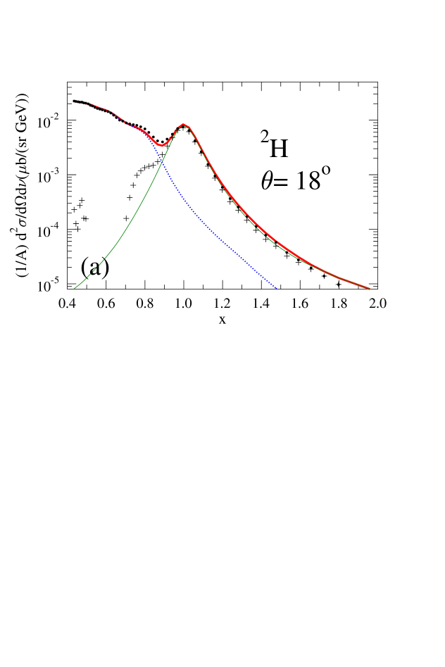
Figure 1a: $\sigma^{tot}$ for inclusive scattering of $E=5.76$ GeV electrons on D; $\theta=18^{\circ}$. Heavy dots are data without error bars. Small dots (blue) and thin line (green) are NI^calc and NE^FF, Eqs. (3), (4), (5). Heavy line (red) is their sum. Crosses are NE^extr= data – NI^calc, Eq. (16). Missing crosses indicate data $\leq\rm{NI}^{calc}$.

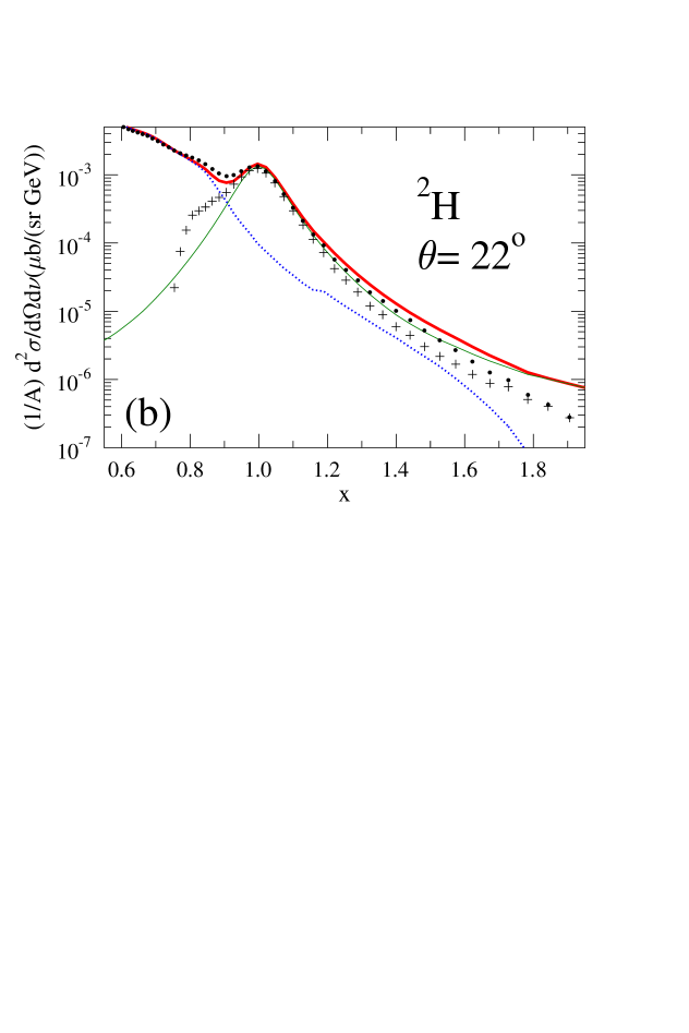
Figure 1b: Fig. 1a for $\theta=22^{\circ}$.

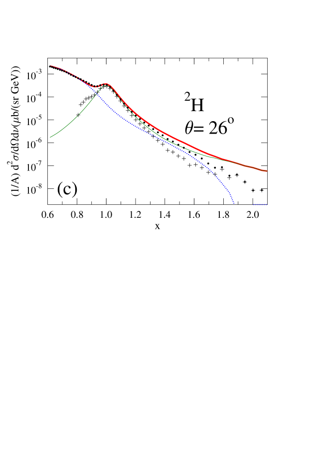
Figure 1c: Fig. 1a for $\theta=26^{\circ}$.

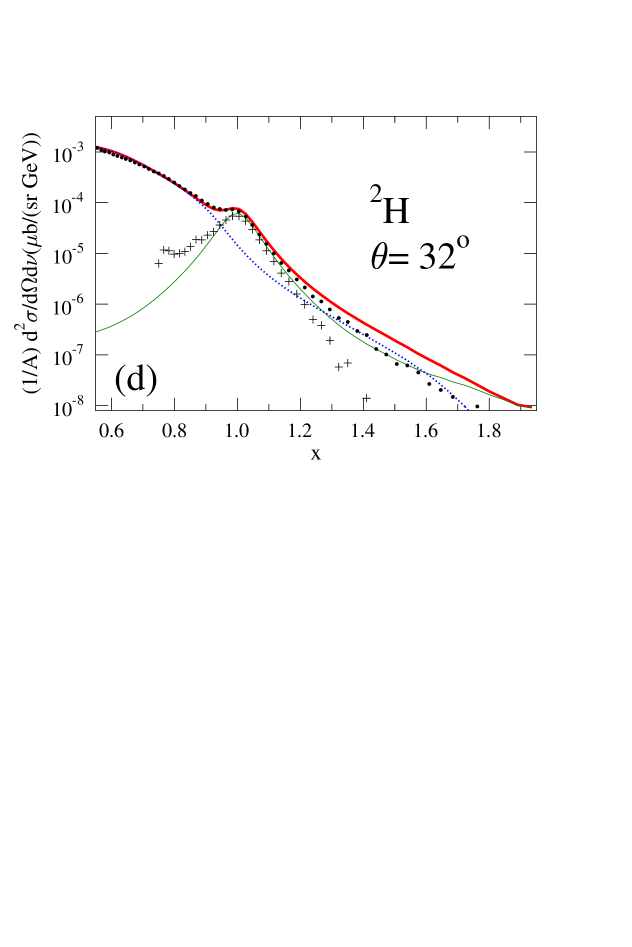
Figure 1d: Fig. 1a for $\theta=32^{\circ}$.

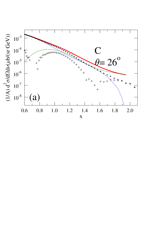
Figure 2a: Fig. 1c for C .

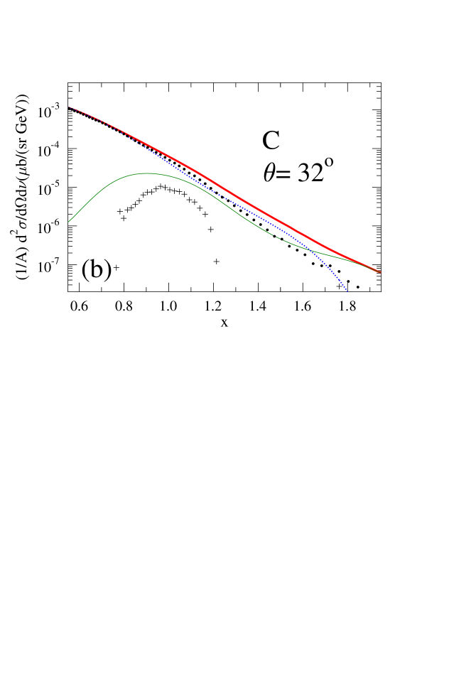
Figure 2b: Fig. 2a for $\theta=32^{\circ}$.

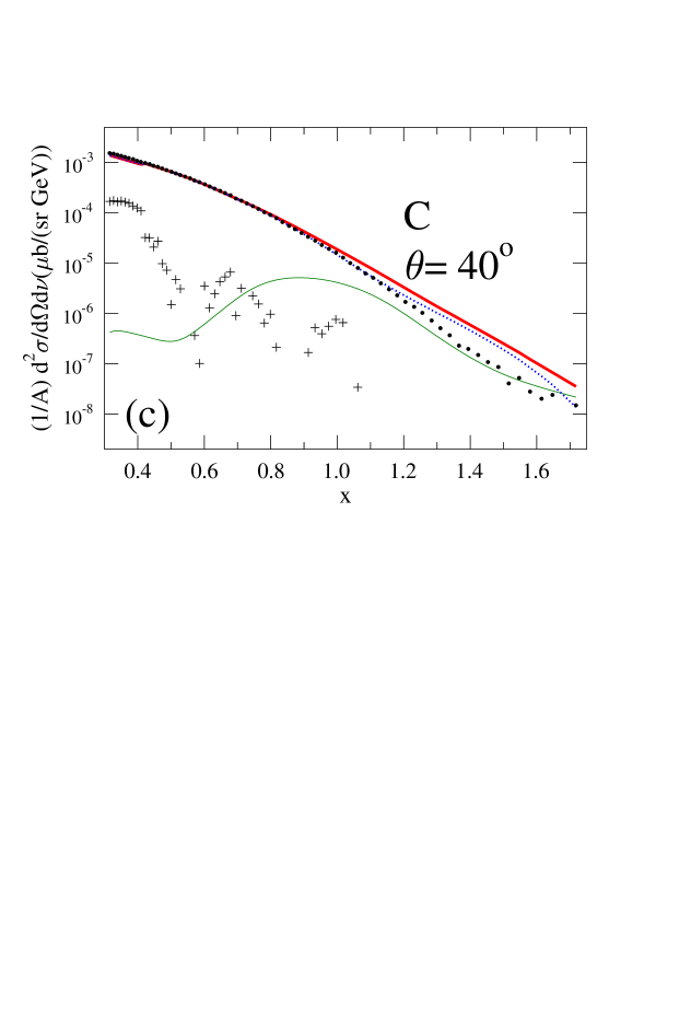
Figure 2c: Fig. 2a for $\theta=40^{\circ}$.

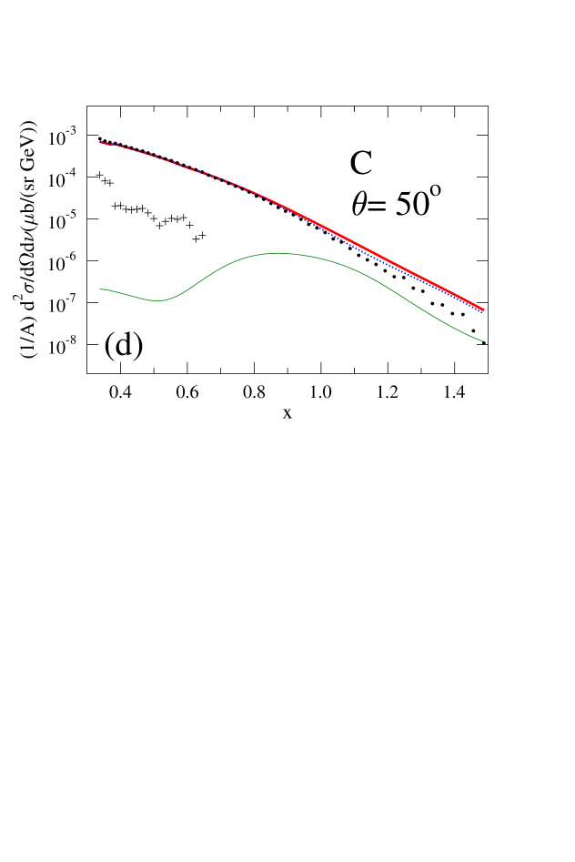
Figure 2d: Fig. 1a for $\theta=50^{\circ}$.

Figure 3a: Linear plot of QE part of total inclusive cross section of $E=5.76$ GeV electrons on D, for $\theta=18^{\circ}$. Drawn line is NE^FF, Eqs. (1.3),( 1.4). Filled circles are ’data’ with total error bars.

Figure 3b: Fig. 3a for $\theta=40^{\circ}$.

Figure 3c: Fig. 3a for C, $\theta=18^{\circ}$.

Figure 3d: Fig. 3c for $\theta=40^{\circ}$.

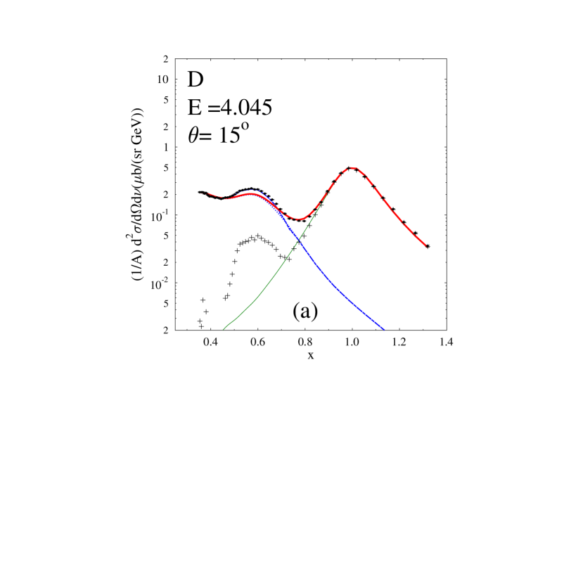
Figure 4a: As Fig. 1a for $E$=4.045 GeV, $\theta=15^{\circ}$ with same meaning of symbols and curves. Dashed curve (blue) is for NI^emp, for which NE${}^{FF}\approx$ NE^extr. (Fig. on log scale from Ref.rtv ).

Figure 4b: Fig. 4a for $\theta=30^{\circ}$ .

Figure 4c: Fig. 1a for $\theta=55^{\circ}$ .

Figure 5a: Distribution functions $f_{p,n}^{{{}^{3}}He}(x,Q^{2}=5$ GeV²). Drawn lines, dashes and dots are for B2(0+1), B2(0) and B2+B3(0+1) .

Figure 5b: Fig. 5a for $Q^{2}=7.5\,$GeV² .

Figure 5c: Comparison of ³He, ³H distribution functions $f_{p}(x,Q^{2}=7.5)$, using B2(0+1).

Figure 6: Computed and extracted $F_{2}^{{}^{3}He}(\theta=40^{\circ})$ for B2+B3 interactions. Lower curve is for $F_{2}^{{}^{3}H}(\theta=40^{\circ})$ .

Figure 7a: Computed total inclusive cross section on ³He for $\theta=18^{\circ}$. ’Data’ with error bars are from ag .

Figure 7b: Fig. 7a for $\theta=40^{\circ}$ .

Figure 8a: EMC data for $\mu^{{}^{4}He}(x\lesssim 1.0,\theta=40^{\circ}$) seely and computed results for fixed $Q^{2}=3.5,5.0$ GeV² rtvemc .

Figure 8b: Fig. a for $\mu^{C}(x\lesssim 1.0,\theta=40^{\circ}$) seely .

Figure 9a: $\mu^{A=3;F_{2}}(\theta=40^{\circ})$ from ratios of SFs $F_{2}$ for ³He and ³H (drawn line and long dashes), and for the iso-scalar component (short dashes) .

Figure 9b: $\mu^{A=3;\sigma}(\theta=40^{\circ})$ from ratios of cross sections. Curves as in Fig. 9a. Empty and full circles are direct data for ³He, respectively manipulated ones for a fictitious iso-scalar A=3 nucleus seely .

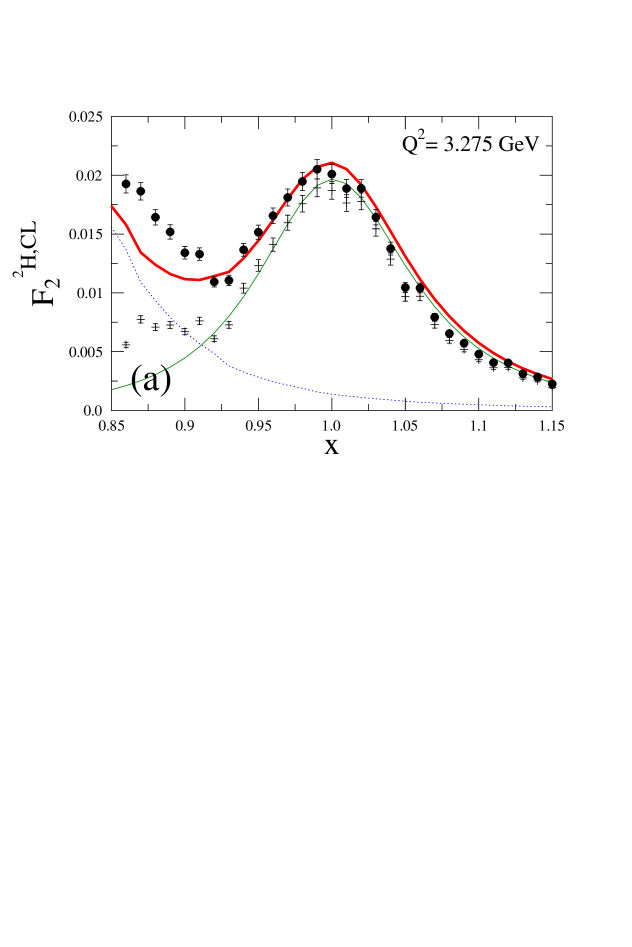
Figure 10a: Filled circles are data with error bars for SF $F_{2}^{D}(x,Q^{2}=3.275\,$GeV${}^{2})$ from CL dataosipd . Symbols and curves as in Fig. 1a .

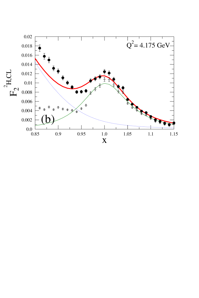
Figure 10b: As Fig.10a for $Q^{2}=4.175$ GeV².

Figure 11: Averaged reduced neutron magnetic $\alpha_{n}$ (Table II). On the curve for OD filled circles are results from CL (Section III), crosses from Lung lung , and diamonds for all results from Table I in Ref. rtv for $Q^{2}\geq 2.5$ GeV². Open circles are from a $D(e,e^{\prime}n)p/D(e,e^{\prime}p)n$ experiment (Fig. 4 , Ref. brooks .

Figure 12a: Extracted $C(x,Q^{2}=2.5\,{\rm GeV}^{2})$ for $x_{M}=0.75$ (short dashes) and $F_{2}^{p,n}(x,Q^{2}=2.5\,{\rm GeV}^{2})$ (drawn and dashed curves).

Figure 12b: As Fig. 12a for $Q^{2}=7.5\,{\rm GeV}^{2}$.

References

- (1) I. Niculescu . Phys. Rev. Lett. 85, 1182 (2000).
- (2) J. Arrington , Phys. Rev. C 64, 014602 (2001).
- (3) S. Rock, , Phys. Rev. Lett. 49, 1139 (1982); Phys. Rev. D 46, 24 (1992).
- (4) D.B. Day , Phys. Rev. C 48, 1849 (1993).
- (5) J. Arrington , Phys. Rev. Letters 82, 2056 (1999); Phys. Rev. C 53, 2248 (1996).
- (6) J. Seely Phys. Rev. Lett. 103, 202301 (2010).
- (7) J. Arrington and D. Gaskell, private communications; [www.jlab.org/ gaskelld/XEMPT/ lightnucleipaper/crosssections].
- (8) P. Solvignon, ETC∗ Workshop, June 4-9 2008, Trento, IT.
- (9) O. Benhar , Phys. Rev. C 44, 2328 (1991); Phys. Lett. B 489, 231 (2000); Phys. Rev. C 67, 014605 (2003).
- (10) P. Fernandez de Cordoba , Nucl. Phys. A 611, 514 (1996).
- (11) A.S. Rinat and M .F. Taragin, Nucl. Phys. A 571, 733 (1994); A 598, 349 (1996); A 620, 417 (1997) (Erratum A 624, 773 (1997)); Phys. Rev. C 60, 044601 (1999).
- (12) S.A. Gurvitz and A.S. Rinat, Phys. Rev. C 65, 024310 (2002).
- (13) M. Osipenko ,[arXiv:hep-ph/0506004], CLAS-NOTE-2005-013; Phys. Rev. C 73, 045205 (2006; [arXiv:hep-ph/0507048].
- (14) S.V. Akulinichev, S.A. Kulagin and G.M. Vagradov, Phys. Lett.B 158, 485 (1985).
- (15) G.B. West, Ann. of Phys. (NY) 74, 646 (1972); W.B. Atwood and G.B. West, Phys. Rev. D 7, 773 (1973)
- (16) M.M. Sargassian, S. Simula and M.I. Strikman, Phys. Rev. C 66, 024001 (2002).
- (17) S.A. Kulagin, G. Piller and W. Weise. Phys. Rev. C 50, 1154 (1994); S.A. Kulagin, [arXiv:hep-ph/9812502]; G. Piller and W. Weise, Phys. Reports 330, 1 (2000).
- (18) Y. Liang , [arXiv:nucl-exp/0410027]; M.E. Christy, private communication. See also hallcweb.jlab.org/res.
- (19) M. Arneodo , Phys. Lett. B 364, 107 (1995).
- (20) A.S. Rinat and M.F. Taragin, Phys. Lett. B 551, 284 (2003).
- (21) A.S. Rinat and B.K. Jennings, Phys. Rev. C 59, 3371 (1999).
- (22) M. Viviani, A. Kievsky and A.S. Rinat, Phys. Rev. C 67, 034003 (2003).
- (23) S.A. Gurvitz, Phys. Rev. C 42, 2653 (1990).
- (24) J. Negele and D. Vautherin, Phys. Rev. C 5, 1472 (1972); Nucl. Phys. A 549, 498 (1992).
- (25) A.S. Rinat, M.F. Taragin and M. Viviani, Phys. Rev. C 70, 014003 (2004); Nucl. Phys. A 784, 25 (2007),
- (26) M. Jones , Phys. Rev. Lett. 84, 1398 (2000); Third Workshop on ’Perspective in Hadronic Physics’, Trieste 2001, IT; Phys. Rev. Lett. 88, 092301 (2002).
- (27) P.A.M. Guichon and M. Vanderhaegen, Phys. Rev. Lett. 91, 142303 (2003); Y.C. Chen , Phys. Rev. Lett. 93, 122301 (2004); P.G. Blunden, W. Melnitchouk, and J.A. Tjon, , C 91, 034612 (2005).
- (28) J. Arrington, W. Melnitchouk and J.A. Tjon, Phys. Rev. C 76, 035205 (2007).
- (29) H. de Vries , Tables IV, V in Atomic and Nuclear Tables 36, 496 (1987)
- (30) A. Kievsky, E. Pace, G. Salme and M. Viviani, Phys. Rev. C 56, 64 (1997).
- (31) R.B. Wirenga, V.G.J. Stoks, and R. Schiavilla, Phys. Rev. C 51, 38 (1995).
- (32) B.S. Pudliner , Phys. Rev. 56, 1720 (1997).
- (33) A.S. Rinat, M.F. Taragin and M. Viviani, Phys. Rev. C 72, 015211 (2005).
- (34) S.A. Kulagin and R. Petti, Nucl. Phys. A 765, 126 (2006).
- (35) G.G. Petratos , Proceedings of the Workshop on Eperiments with Tritium at JLab (1999).
- (36) E. Pace, G. Salme, S. Scopetta and A. Kievsky, Phys. Rev. C 64, 055203 (2001); Nucl. Phys. A 689, 453 (2001).
- (37) I.R. Afnan , Phys. Rev. 68, 035201 (2003).
- (38) W. Brooks, Nucl. Phys. A 750, 261 (2005); J. Lachniet , Phys. Rev. Lett. 102, 192001 (2009).
- (39) A. Lung, Phys. Rev. Lett. 70, 718 (1993).
- (40) J.P.B.C. Melo , Phys. Lett. B 671, 153 (2009).
- (41) W. Melnitchouk and A.W. Thomas, Phys. Lett. B 377 11 (1996).
- (42) Y. Kahn, W. Melnitchuk and S.A. Kulagin, [arXiv:0809.4308v1 [nucl-th]].
- (43) J. Arrington, F. Coester, R. J. Holt and T.-S. Lee, [arXiv:0805.3116v2 [nucl-th]].
- (44) M. Osipenko , Nucl. Phys. A 766, 142 (2006).
- (45) J. Arrington, private communication.
- (46) R. L. Jaffe, Proceedings Los Alamos Summer School, 1985; Ed. M. Johnson, A. Picklesimer (Wiley; NY, 1986).
- (47) G.B. West, Interactions between Particles and Nuclear Physics. Ed. R.E. Mischke, AIP (NY 1984), p.360.
- (48) A.S. Rinat and M.F. Taragin, Phys. Rev. C 73, 045201 (2006).
- (49) A.S. Rinat and M.F. Taragin, Phys. Rev. C 72, 065209 (2005);