A Poisson-Boltzmann approach for a lipid membrane in an electric field

Abstract

The behavior of a non-conductive quasi-planar lipid membrane in an electrolyte and in a static (DC) electric field is investigated theoretically in the nonlinear (Poisson-Boltzmann) regime. Electrostatic effects due to charges in the membrane lipids and in the double layers lead to corrections to the membrane elastic moduli which are analyzed here. We show that, especially in the low salt limit, i) the electrostatic contribution to the membrane’s surface tension due to the Debye layers crosses over from a quadratic behavior in the externally applied voltage to a linear voltage regime. ii) the contribution to the membrane’s bending modulus due to the Debye layers saturates for high voltages. Nevertheless, the membrane undulation instability due to an effectively negative surface tension as predicted by linear Debye-Hückel theory is shown to persist in the nonlinear, high voltage regime.

1 Introduction

Bilayers formed from lipid molecules are an essential component of the membranes of biological cells. The mechanical properties of membranes at equilibrium are characterized by two elastic moduli, the surface tension and the bending modulus [1]. These moduli typically depend on electrostatic properties, and their modifications in case of charged membranes/surfaces in an electrolyte have been examined theoretically in the period 1980-90’s as reviewed e.g. in Ref. [2]: they have been first derived by Winterhalter and Helfrich [3] within linearized Debye-Hückel (DH) approximation, then by Lekkerkerker [4] in the nonlinear Poisson-Boltzmann (PB) regime for charged monolayers and by Ninham et al. [5] for charged symmetric bilayers. Later on Helfrich et al. revisited the question of the electrostatic corrections to the bending modulus of charged symmetric bilayers [6].

Nowadays, the study of deformations of membranes or vesicles in electric fields is an active field of research linked to many biotechnological applications. For instance, the application of electric fields is used to produce artificial vesicles from lipid films (electroformation), or to create pores in vesicles (electroporation), which is an important route for drug delivery. Both processes are widely used experimentally although they are not well understood theoretically. The effects of electric fields on giant unilamellar vesicles have been reviewed recently in Ref. [7]. This system shows a rich panel of possible behaviors and morphological transitions depending on experimental conditions – electric field frequency, conductivities of the medium and of the membrane, salt concentration, etc. These observations are supported to a large extend by theoretical modeling [8].

Originally it was Helfrich et al. who pointed out that the deformation of lipid vesicles in electric fields can serve as a means to determine the electrostatic corrections to the membrane elastic moduli [9]. Besides this observation on the macroscopic scale other techniques can provide valuable insights into the moduli corrections such as AFM, impedance spectroscopy [10], neutron reflectivity [11] and X-ray scattering [12]. Recently [12], X-ray scattering experiments have been carried out on a system of two superposed lipid membranes in an AC electric field. In trying to analyze this data, we noted that these experiments have been carried out at relatively high voltages, in a regime where the linearized DH approach may not be applicable. In order to describe such a situation theoretically, we extend previous work [13, 14, 15] based on the DH approach to the nonlinear PB regime, which is more suitable for realistic situations in which the induced surface charges on the membrane are large.

In this paper, we present a simple approach to calculate electrostatic corrections in the elastic moduli of a quasi-planar lipid membrane. The membrane is assumed to be non-conductive to ions, non-permeable to water and electrically neutral, it is subjected to a normal DC electric field and embedded in an electrolyte described by the Poisson-Boltzmann equation. In this situation, the electric field leads to an accumulation of charges on both sides of the membrane, which affect the mechanical properties of the membrane. The electrostatic corrections to the elastic moduli can be used to analyze the instability of a lipid membrane in an applied DC electric field. In contrast to previous work, based on a free energy approach [4, 6, 16], our method is based on a calculation of the stress (or force) balance at the membrane surface using electrokinetic equations [17]. This method is related to the work of Kumaran [18] who used a similar approach in the context of equilibrium charged membranes. Two points are worth mentioning: first, our approach is able to describe the capacitive effects of the membrane and of the Debye layers while keeping the simplicity of the zero thickness approximation on which most of the literature on lipid membranes is based. Second, our approach can include non-equilibrium effects which can not be described within the free energy approach. For instance, in Refs. [13, 14, 15] we investigated the effects of ionic currents flowing through the membrane, which in turn affect the fluid flow near the membrane. Other types of non-equilibrium effects that could be included in that framework are those arising from the stochasticity of ion channels.

2 Model equations

We consider a steady (DC) voltage $V$ between two electrodes at a fixed distance $z=\pm L/2$, applied to an initially flat membrane located at $z=0$. The membrane is embedded in an electrolyte of monovalent ions with densities $n^{+}$ and $n^{-}$. The membrane is treated as non-conductive for both ion species and is (effectively) uncharged; thus we focus solely on capacitive effects. A point on the membrane is characterized within the Monge representation by a height function $h(\mathbf{r}_{\perp})$, where $\mathbf{r}_{\perp}$ is a two-dimensional in-plane vector in the membrane.

In the electrolyte, the electric potential $\phi$ obeys Poisson’s equation

$$\nabla^{2}\phi=-\frac{1}{\epsilon}\left(en^{+}-en^{-}\right)=-\frac{2}{\epsilon}\rho\,.$$ (1)

Here $e$ is the elementary charge, $\epsilon$ is the dielectric constant of the electrolyte and we have introduced half of the charge density,

$$\rho=e\frac{n^{+}-n^{-}}{2}\,.$$ (2)

For the sake of simplicity, we assume a symmetric $1:1$ electrolyte, so that far away from the membrane $n^{+}=n^{-}=n^{*}$, and the total system is electrically neutral.

The densities of the ion species obey the Poisson-Nernst-Planck equations

$$\partial_{t}n^{\pm}+\nabla\cdot\mathbf{j}^{\pm}=0\,,$$ (3)

with ionic current densities

$$\mathbf{j}^{\pm}=D\left(-\nabla n^{\pm}\mp n^{\pm}\frac{e}{k_{B}T}\nabla\phi\right)\,,$$ (4)

where $k_{B}T$ is the thermal energy. For simplicity we consider the case where both ion types have the same diffusion coefficient $D$ and neglected various corrections for concentrated solutions [19].

As boundary conditions (BC), the potential at the electrodes is externally held at

$$\phi\left(z=\pm\frac{L}{2}\right)=\pm\frac{V}{2}\,.$$ (5)

This BC is oversimplified for real electrodes, but captures the main effects of the electric field, see the discussion in Ref. [15]. The distance between the electrodes is assumed to be much larger than the Debye length, $L\gg\lambda_{D}=\kappa^{-1}$. In that case, the bulk electrolyte is quasi-neutral, $n^{+}=n^{-}=n^{*}$, with negligible charge density (compared to the total salt concentration), so that far from the membrane

$$\rho\left(z=\pm\frac{L}{2}\right)=0\,.$$ (6)

The BC at the membrane is crucial to recover the correct physical behavior. Let $\mathbf{n}$ be the unit vector normal to the membrane. We use the Robin-type BC

$$\lambda_{m}(\mathbf{n}\cdot\nabla)\phi_{|z=h^{+}}=\lambda_{m}(\mathbf{n}\cdot\nabla)\phi_{|z=h^{-}}=\phi(h^{+})-\phi(h^{-})\,,$$ (7)

where

$$\lambda_{m}=\frac{\epsilon}{\epsilon_{m}}d$$ (8)

is a length scale that contains the membrane thickness $d$ and the ratio of the dielectric constant of the electrolyte, $\epsilon$, and of the membrane, $\epsilon_{m}$. This BC was originally developed for electrodes sustaining Faradaic current [20, 21] or charging capacitively [22]. In Refs. [23, 14, 15], this BC was derived, and was shown to properly account for the jump in the charge distribution which occurs near the membrane as a result of the dielectric mismatch between the membrane and the surrounding electrolyte.

3 Poisson-Boltzmann approach for a membrane in an external potential

Here we show how the well-known solution of the Poisson-Boltzmann (PB) equation for a single charged plate in an electrolyte can be used to describe the present situation of a capacitive membrane with induced Debye layers in an external potential.

In a steady state situation and when there is no electric current through the membrane, one obtains from Eqs. (3, 4)

$$-\nabla n^{\pm}\mp n^{\pm}\frac{e}{k_{B}T}\nabla\phi=0\,.$$ (9)

After a direct integration using the BCs from above, one obtains

$$n^{\pm}=n^{*}\rme^{\mp\frac{e}{k_{B}T}\left(\phi(z)-\frac{V}{2}\right)}\,,$$ (10)

and insertion in Poisson’s equation then yields the Poisson-Boltzmann (PB) equation

$$\nabla^{2}\phi=\frac{2n^{*}e}{\epsilon}\sinh\left[\frac{e}{k_{B}T}\left(\phi(z)-\frac{V}{2}\right)\right]\,.$$ (11)

Linearization (for $\phi-\frac{V}{2}\ll 1$) leads to the well-known Debye-Hückel (DH) equation,

$$\nabla^{2}\phi=\kappa^{2}\left(\phi(z)-\frac{V}{2}\right)\,,$$ (12)

where

$$\kappa^{2}=\frac{2e^{2}n^{*}}{\epsilon k_{B}T}$$ (13)

and $\kappa^{-1}=\lambda_{D}$ is the Debye length that defines the characteristic length scale for charge relaxation in the electrolyte.

The nonlinear PB equation (11) for the planar case can be integrated analytically [2], leading to

$$\phi(z) = -\frac{2k_{B}T}{e}\ln\left(\frac{1+c\rme^{-\kappa z}}{1-c\rme^{-\kappa z}}\right)+\frac{V}{2}\,,$$ (14)

$$n^{\pm}(z) = n^{*}\left(\frac{1\pm c\rme^{-\kappa z}}{1\mp c\rme^{-\kappa z}}\right)^{2}\,,$$ (15)

for $z>0$. The expressions for $z<0$ can be obtained using the symmetry of the system: $\phi(-z)=-\phi(z)$, $n^{\pm}(-z)=-n^{\pm}(z)$.

Just as in the classical PB solution for a single charged plate in contact with an electrolyte, the non-dimensional parameter $c$ is determined by the BC for the potential at the membrane. For a flat charged surface surrounded by an electrolyte [2], $c$ is given by a simple quadratic equation and can be expressed in terms of the ratio of the two characteristic length scales: the Gouy-Chapman length $b=\frac{2\epsilon k_{B}T}{e|\sigma|}$ (with $|\sigma|$ the charge density of the surface) and the Debye length $\lambda_{D}=\kappa^{-1}$. In contrast, in the case of a membrane in an electric field, we obtain from Eq. (7) the following nonlinear equation

$$4\kappa\lambda_{m}\frac{c}{c^{2}-1}+\frac{eV}{k_{B}T}=4\ln\left(\frac{1+c}{1-c}\right)\,.$$ (16)

Note that two dimensionless parameters enter this equation: the ratio of electrostatic to thermal energy,

$$\bar{V}=\frac{eV}{k_{B}T}\,,$$ (17)

and the dimensionless parameter [21]

$${\bar{\lambda}}_{m}=\kappa\lambda_{m}=\frac{\lambda_{m}}{\lambda_{D}}=\frac{\epsilon\kappa}{\epsilon_{m}/d}=\frac{C_{D}}{C_{m}}\,,$$ (18)

which quantifies the electrical coupling between the membrane and the Debye layers. More precisely, depending on whether this parameter is large or small with respect to one, the capacitance of the diffuse part of the double layer, $C_{D}=\epsilon\kappa$, or the capacitance of the membrane, $C_{m}=\epsilon_{m}/d$, dominates the overall voltage drop.

The non-dimensional parameter $c=c(\bar{\lambda}_{m},\bar{V})$ which is determined by Eq. (16) is related to the potential at the membrane, $\phi(0^{+})$, and to the charge density at the membrane, $\rho(0^{+})$, by the following relations

$$\phi(0^{+})=-\frac{4k_{B}T}{e}{\rm artanh}(c)+\frac{V}{2}\,,$$ (19)

$$\rho(0^{+})=en^{*}\sinh\left[4\,{\rm artanh}(c)\right]\,.$$ (20)

From Eq. (19), one can see that the values of $c$ must be restricted to the interval $[0,1]$. In the limit of small voltages, $\bar{V}\ll 1$, there is a linear relation between $c$ and the charge distribution at the membrane, since $c=\frac{\rho(0^{+})}{4en^{*}}=\frac{\epsilon\kappa^{2}V}{8en^{*}(2+\kappa\lambda_{m})}$, in accordance with the calculations based on the DH approximation of Ref. [15].

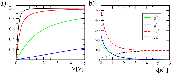
Figure 1: a) Solution of Eq. (16) for different amounts of salt: $\kappa=10^{6}{\rm m}^{-1}$ (pure water; black), $\kappa=10^{7}{\rm m}^{-1}$ (red), $\kappa=10^{8}{\rm m}^{-1}$ (green), $\kappa=10^{9}{\rm m}^{-1}$ (blue). b) Charge distribution (in units of ${\rm Cm}^{-3}$) for $z>0$ : comparison of the nonlinear solution (blue) with the linearized Debye-Hückel solution (green). The asymmetric distribution of positive (red dashed) and negative charges (black dashed) for the nonlinear solution is also shown. Parameters used: $\epsilon=80\epsilon_{0}$ (water) and $\epsilon_{m}=2\epsilon_{0}$ for the membrane. As the membrane thickness is typically $d=5{\rm nm}$ this leads to $\lambda_{m}=\frac{\epsilon}{\epsilon_{m}}d=200{\rm nm}$. For b) we used $\kappa=10^{6}{\rm m}^{-1}$, corresponding to $en^{*}\simeq 9.16\,{\rm Cm}^{-3}$, and $V=0.1V$.

Fig. 1a) shows the solution $c$ of Eq. (16) as a function of external voltage for various values of $\kappa$, which corresponds to varying the amount of salt since $\kappa\propto\sqrt{n^{*}}$. Clearly, for low salt, the linear approximation remains valid only for rather small voltages (for instance it holds only for $V\lesssim 0.1{\rm V}$ in pure water), while for high salt $V=5{\rm V}$ is still in the linear regime. Fig. 1b) shows a comparison of the charge distribution for the nonlinear PB (blue) and the linear DH solution (green). As expected, the figure shows that the DH approximation underestimates the surface charge on the membrane layers as compared to the PB calculation. The figure also shows the distribution of the positive and negative ions, which both tend to $n^{*}$ far from the interface as a result of electroneutrality.

Although the present situation differs from the case of a single charged plate in an PB electrolyte, the structure of the solutions Eqs. (14, 15) is very similar in both problems. Because of this, there is an equivalent to the Contact theorem [2], which relates in the single charged plate problem the surface charge density to the limiting value of the potential/ionic density at the plate: namely, one can give the effective surface charge $\sigma_{\rm eff}$ for the charged plate problem that creates the same voltage/charge distributions as the capacitive membrane in the external field. This effective surface charge reads

$$\sigma_{\rm eff}^{2}=4\epsilon n^{*}k_{B}T\left[\cosh\left(\frac{e}{k_{B}T}(\phi(0^{+})-V/2)\right)-1\right]\,.$$ (21)

4 Corrections to membrane elastic moduli

Surface tension. The electrostatic corrections to the surface tension can be calculated directly from the stresses acting on the membrane in the flat configuration (also called the base state) as explained in Refs. [24, 15]. The total stress tensor reads

$$\tau_{ij}=-p\delta_{ij}+\eta\left(\partial_{i}v_{j}+\partial_{j}v_{i}\right)+\epsilon\left(E_{i}E_{j}-\frac{1}{2}\delta_{ij}E^{2}\right)\,$$ (22)

which contains the pressure, the viscous stresses in the surrounding fluid (the electrolyte) and the Maxwell stress due to the electrostatic field. $\eta$ is the viscosity of the electrolyte and $\mathbf{v}$ its velocity field. The electric field is given by $\mathbf{E}=-\nabla\phi$.

In the base state, the electric field is oriented in $z$-direction, and the condition $\nabla\cdot\tau=0$ implies that $\partial_{z}p=\frac{\epsilon}{2}\partial_{z}\left(\left(\partial_{z}\phi\right)^{2}\right)=-2\rho\partial_{z}\phi$. Using Eqs. (14, 15) and imposing $p(z\rightarrow\infty)=0$, this is readily solved by

$$p(z>0)=16n^{*}k_{B}Tc^{2}\frac{\rme^{2\kappa z}}{\left(c+\rme^{\kappa z}\right)^{2}\left(c-\rme^{\kappa z}\right)^{2}}\,,$$ (23)

and similarly with $z\rightarrow-z$ for $z<0$.

Let us call $S$ a closed surface englobing the membrane with the normal vector field ${\bf n}$. The force acting on the surface $S$ in the ${\bf x}$-direction (chosen to be the direction of the lateral stress) can be calculated from the stress tensor as $F_{x}=\int_{S}{\bf x}\cdot\tau\cdot{\bf n}\,\,dS$. Since $\tau$ is divergence free, the surface $S$ can be deformed, for convenience to a cube of size $L$, and it is easy to see that the integral is non-zero only on the faces of the cube with the normal along $\pm{\bf x}$. With $dS=Ldz$ and $\Delta\Sigma=F_{x}/L$ for ${\bf n}=+{\bf x}$, we arrive at

$$\Delta\Sigma=\int_{-L/2}^{L/2}\tau_{xx}(z)dz\,.$$ (24)

From Eq. (22), one has $\tau_{xx}(z)=-p(z)-\frac{\epsilon}{2}(\partial_{z}\phi)^{2}$, where $\phi(z)$ and $p(z)$ are the potential and the pressure in the base state given above. Upon integration (using $L\kappa\gg 1$), one obtains the corrections to the surface tension, as a sum of two terms.

First, there is the external contribution due to the Debye layers,

$$\Delta\Sigma_{\kappa}=-\frac{32n^{*}k_{B}T}{\kappa}\frac{c^{2}}{1-c^{2}}\,.$$ (25)

Second, there is the internal contribution due to the electric field inside the membrane (cf. Ref. [15]), which is given by $E_{0}^{m}=-\frac{1}{d}\left(\phi(0^{+})-\phi(0^{-})\right)$. That correction to the surface tension is $\Delta\Sigma_{m}=-\epsilon_{m}d\left(E_{0}^{m}\right)^{2}$, or explicitly

$$\Delta\Sigma_{m}=-\frac{\epsilon_{m}}{d}\left[-\frac{4k_{B}T}{e}\ln\left(\frac{1+c}{1-c}\right)+V\right]^{2}\,.$$ (26)

Note that both corrections to the surface tension are negative, which means that these corrections can lead to an instability as soon as the total surface tension $\Sigma_{tot}=\Sigma_{0}+\Delta\Sigma_{\kappa}+\Delta\Sigma_{m}$ (which is the sum of the bare tension $\Sigma_{0}$ plus the above corrections) becomes negative [25].

Bending modulus. To obtain the correction to the bending modulus we perform, as detailed in Ref. [15] for the DH case, a calculation of the potential at first order in the membrane height. Then, by solving the hydrodynamics problem of the electrolyte around the membrane (in Stokes approximation), one determines the pressure and obtains the total stress tensor. The growth rate of membrane fluctuations, $s(k_{\perp})$, where $\mathbf{k}_{\perp}$ is the wave vector in the membrane plane, is then determined by imposing that the discontinuity of the normal-normal component of the total stress tensor at the membrane has to equal the membrane restoring force:

$$-\left[(\tau_{zz,1}(z=0+)-\tau_{zz,1}(z=0-)\right]=-\frac{\partial F_{H}}{\partial h(\mathbf{r}_{\perp})}\,.$$ (27)

Here $F_{H}$ is the standard Helfrich free energy,

$$F_{H}=\frac{1}{2}\int d^{2}\mathbf{r}_{\perp}[\Sigma_{0}\left(\nabla h\right)^{2}+K_{0}\left(\nabla^{2}h\right)^{2}],$$ (28)

and $\Sigma_{0}$ and $K_{0}$ are the bare surface tension and the bare bending modulus of the membrane, respectively. Expanding the left hand side of Eq. (27) in powers of $\mathbf{k}_{\perp}$ yields the growth rate of the form

$$\eta k_{\perp}s(k_{\perp})=-\frac{1}{4}\left(\Sigma_{0}+\Delta\Sigma_{\kappa}+\Delta\Sigma_{m}\right)k_{\perp}^{2}-\frac{1}{4}\left(K_{0}+\Delta K_{\kappa}+\Delta K_{m}\right)k_{\perp}^{4}\,.\quad\quad\quad$$ (29)

Details of the calculations can be found in A. The surface tension corrections calculated above in Eqs. (25, 26) can be recovered by this method, which provides a self-consistency check. For the bending modulus one obtains

$$\Delta K_{\kappa} = \frac{8n^{*}k_{B}T}{\kappa^{3}}\frac{c^{2}(3-c^{2})}{1+c^{2}}\,,$$ (30)

$$\Delta K_{m} = -\epsilon_{m}\left(E^{0}_{m}\right)^{2}\left[-\frac{d^{3}}{12}+\frac{2k_{B}T}{E^{0}_{m}e\kappa}\frac{c(1-c^{2})}{1+c^{2}}d\right]\,,$$ (31)

for the external contribution due to the Debye layers and the internal contribution due to the voltage drop at the membrane, respectively. The field inside the membrane is given by $E_{0}^{m}=-\frac{1}{d}\left[-\frac{4k_{B}T}{e}\ln\left(\frac{1+c}{1-c}\right)+V\right]$.

5 Discussion

Let us now discuss the nonlinear electrostatic effects on the membrane elastic moduli in the limits of low and high applied voltages.

Low voltage regime. In the low voltage limit, $\bar{V}\ll 1$, a solution of Eq. (16) to linear order in $c$, yields

$$c=\frac{\bar{V}}{4(2+\bar{\lambda}_{m})}=\frac{1}{4(2+\lambda_{m}\kappa)}\frac{eV}{k_{B}T}=\frac{\rho(0^{+})}{4en^{*}}\,.$$ (32)

Here $\rho(0^{+})$ is half the charge density at the membrane, corresponding to the quantity called $\rho_{m}$ in Ref. [15] for the DH case. Expanding $\phi(z)$ and $\rho(z)$, as well as the corrections to the moduli $\Delta\Sigma_{\kappa}$, $\Delta\Sigma_{m}$, $\Delta K_{\kappa}$ and $\Delta K_{m}$ for small $c$, one exactly recovers all of the results given in Ref. [15]. Specifically, all corrections to the moduli scale quadratically with the external voltage, $\propto V^{2}$. This is due to the fact that both the potential and the induced charge are proportional to the applied voltage.

High voltage regime. In the opposite limit, $\bar{V}\gg 1$ implies $c\rightarrow 1$. Introducing $\alpha=1-c$ and expanding Eq. (16) for small $\alpha$, one gets $-\frac{2\bar{\lambda}_{m}}{\alpha}+4\ln\alpha+\bar{V}+\bar{\lambda}_{m}-4\ln 2=0$. For high values of $\bar{V}$ one can neglect the last two (constant) terms and gets

$$c=1-\frac{\frac{1}{2}\bar{\lambda}_{m}}{W\left(\frac{1}{2}\bar{\lambda}_{m}\rme^{\bar{V}/4}\right)}\simeq 1-\frac{\frac{1}{2}\bar{\lambda}_{m}}{\bar{V}/4}\,,$$ (33)

where $W(x)$ is Lambert’s function, i.e. $y=W(x)$ is the solution of $ye^{y}=x$.

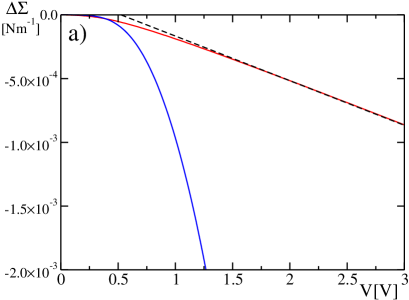
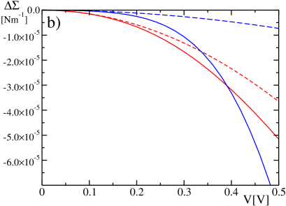
Figure 2: Corrections to the surface tension for $\kappa=10^{6}{\rm m}^{-1}$ (pure water) as a function of voltage. Corrections from the Debye layer are in red, corrections due to the voltage drop at the membrane are in blue. a) Nonlinear PB result. One sees that the correction due to the Debye layer scales linearly in the voltage for high voltages (cf. the black dashed straight line), while the contribution from inside the membrane scales quadratically in the voltage. b) Comparison of the nonlinear PB result (solid lines) with the linear DH result (dashed lines).

As a result, the nonlinear electrostatics strongly effects the corrections to the moduli from the Debye layers. In fact, the external contribution to the surface tension scales as

$$\Delta\Sigma_{\kappa}(\bar{V}\gg 1)\propto-\frac{c^{2}}{1-c^{2}}\rightarrow-\frac{\bar{V}}{4\bar{\lambda}_{m}}\,$$ (34)

instead of $\Delta\Sigma_{\kappa}(\bar{V}\ll 1)\propto-\frac{\bar{V}^{2}}{(2+\bar{\lambda}_{m})^{2}}$ : in the high voltage regime, the external surface tension correction scales linearly with the voltage instead of quadratically. The crossover from $\bar{V}^{2}$ to $\bar{V}$ is salt dependent, i.e. depends on the value of $\bar{\lambda}_{m}=\lambda_{m}\kappa$, cf. Fig. 1. In contrast, the external surface tension correction $\Delta\Sigma_{m}$ remains a quadratic function of the applied voltage.

Fig. 2 displays both corrections to the surface tension as a function of voltage for low salt (pure water). Fig. 2a) shows that due to the crossover to a linear voltage dependence for the external surface tension correction, rapidly $\Delta\Sigma_{m}$ (the blue curve) wins and $\Delta\Sigma_{\kappa}$ (red curve) becomes negligible for $V\gtrsim 1.5V$. Fig. 2b) shows a comparison of the nonlinear PB result (solid lines) with the linear DH result (dashed lines). For $V\lesssim 0.2V$, there is agreement and the external contribution dominates. However, for higher voltages the linearized DH solution becomes completely misleading: it predicts that $|\Delta\Sigma_{\kappa}|>|\Delta\Sigma_{m}|$ for all voltages (and both proportional to $V^{2}$), while already above $V\gtrsim 0.4V$ the internal contribution exceeds the external contribution.

For the bending modulus corrections, the differences between the DH and PB models are even more striking: As a function of the applied voltage, the external contribution levels off at a constant value

$$\Delta K_{\kappa}(\bar{V}\gg 1)=\frac{8n^{*}k_{B}T}{\kappa^{3}}\frac{c^{2}(3-c^{2})}{1+c^{2}}\rightarrow\frac{8n^{*}k_{B}T}{\kappa^{3}}\,.$$ (35)

In contrast, the internal contribution $\Delta K_{m}$ continues to grow quadratically in the high voltage limit. Fig. 3a) and b) show comparisons of the nonlinear PB solutions (solid) and the linear DH solutions (dashed) for both contributions to the bending modulus. Note, however, the different scales: Although the external contribution saturates, see Fig. 3a), this value is larger by two orders of magnitude than the still growing value from the internal contribution, cf. Fig. 3b). In conclusion, for pure water and voltages $\simeq 0.2-5V$, the total correction to the bending modulus will appear constant within this voltage interval. Only for still higher voltages the quadratic growth due to the internal contribution $\Delta K_{m}$ will dominate.

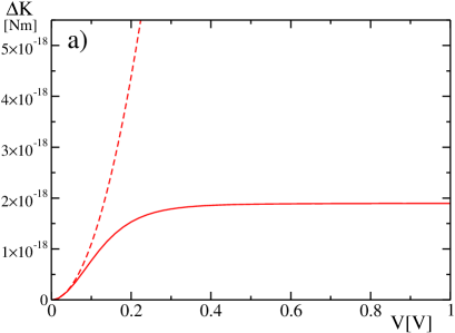
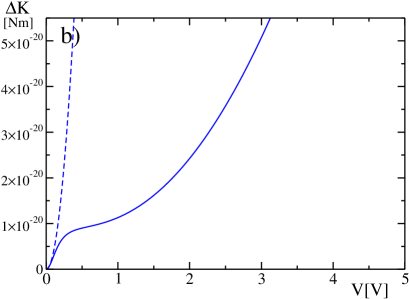
Figure 3: Corrections to the bending modulus for $\kappa=10^{6}{\rm m}^{-1}$ (pure water) as a function of voltage. a) Corrections from the Debye layer. b) Corrections due to voltage drop at the membrane. Nonlinear PB calculations are solid, linearized DH calculations are dashed (note the different scales on the left and right panels).

Membrane instability. Let us briefly discuss the consequences for the membrane undulation instability. As mentioned above, an instability develops in this system when the total surface tension, the sum of the bare value and the electrostatic corrections, becomes negative. The threshold value for the voltage, $V_{c}$, has been calculated in Ref. [15] within linearized DH theory and reads (in case of a non-conductive membrane)

$$V_{c}^{2}=\frac{\Sigma_{0}d\left(2+\kappa\lambda_{m}\right)}{\kappa\left(\kappa\epsilon_{m}\lambda_{m}^{2}+\epsilon d\right)}\,.$$ (36)

This curve is shown in Fig. 4 as the blue line. The red line, in contrast, shows the nonlinear PB result given by numerical solution of $0=\Sigma_{tot}=\Sigma_{0}+\Delta\Sigma_{\kappa}+\Delta\Sigma_{m}$ with Eqs. (25, 26) for the surface tension corrections and $c(\bar{\lambda}_{m},\bar{V})$ calculated from Eq. (16). In the high salt limit, the Debye layers shrink to zero and as a result the external contribution vanishes. For the internal contribution, the inside field is exactly calculated from the DH approach, as can be seen from the behavior of the parameter $c$ in Figure 1a. Thus, both curves merge and attain the limiting value given by Eq. (36), $V_{c}(\kappa\rightarrow\infty)=\sqrt{\frac{\Sigma_{0}d}{\epsilon_{m}}}$. In contrast, for low salt, the linear result overestimates the threshold value, since it underestimates the induced charges at the membrane, as shown in Fig. 1b).

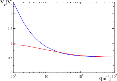
Figure 4: Threshold voltage $V_{c}$ for the membrane undulation instability as a function of salt (i.e. $\kappa$). Nonlinear PB result (red curve) vs. linear DH result (blue curve). Parameters: $\kappa=10^{6}{\rm m}^{-1}$ (pure water); bare surface tension $\Sigma_{0}=10^{-3}{\rm Nm}^{-1}$; $\lambda_{m}=200{\rm nm}$.

In addition to the threshold voltage for the instability, the most unstable wave number associated to the instability will be affected by the electrostatic nonlinearities of the PB equation. This wave vector corresponds to the maximum of the growth rate given by Eq. (29) with respect to $k_{\perp}$. In the low salt regime, since the system is more unstable in the presence of electrostatic nonlinearities, cf. Fig. 4, in general the wave vector will be increased as compared to the predictions from the DH approach.

6 Conclusions

We have investigated the nonlinear electrostatic effects of an external DC electric field on a purely capacitive membrane, which is non-conductive for the ions and bears no fixed charges, in an electrolyte. We have calculated in the nonlinear Poisson-Boltzmann regime the corrections to the membrane elastic moduli – both the external ones due to the Debye layers surrounding the membrane and the internal corrections due to the electric field inside the membrane. Strong deviations from the linear Debye-Hückel behavior have been found in the low salt regime at already rather moderate voltages. In particular we have shown that the external contribution to the surface tension crosses over from a quadratic dependence on the externally applied voltage as predicted by the linearized theory to a linear voltage dependence. In contrast, the internal contribution remains quadratic and becomes dominating at high voltages. The external contribution to the bending modulus even saturates for high voltages, while the internal contribution remains quadratic in voltage.

In addition, our work confirms that the surface tension still grows in absolute value with the voltage, which means that the membrane undulation instability present in the DH theory (due to an effectively negative surface tension) persists in the nonlinear PB regime. The nonlinearities affect the threshold in voltage and the characteristic wavelength of the instability.

The method presented here can serve as a starting point for further extensions. One example would be to include fixed charges in addition to induced charges, similarly as studied in [26]. Another possible direction would be to improve the description of the membrane, cf. the recent work in Ref. [27] where thickness fluctuations of the membrane and fluctuations of the lipid dipole orientations within the membrane are accounted for in a comprehensive continuum model for a membrane in a normal DC electric field. Other possible extensions could include other types of non-linear effects, for example due to membrane elasticity, due to inclusions of proteins such as ion channels or pumps in the membrane [28], and also various relevant non-equilibrium effects, coupling electrostatics and hydrodynamics as in induced charge electro-osmosis [29]. Finally, in the biological context, the heterogeneity of the bilayer composition is another feature which is beyond the present model and which is likely to be important.

Appendix A Details of calculation of bending modulus

As this is the extension to nonlinear electrostatics of earlier work [15], we only sketch the calculations. To solve the electrostatics problem to first order in the membrane height, one linearizes in $h$ by writing

$$\phi(\mathbf{k}_{\perp},z)=\phi_{0}(z)+\phi_{1}(\mathbf{k}_{\perp},z)\,,$$

$$\rho(\mathbf{k}_{\perp},z)=\rho_{0}(z)+\rho_{1}(\mathbf{k}_{\perp},z)\,,$$

$$n^{\pm}(\mathbf{k}_{\perp},z)=n_{0}^{\pm}(z)+n^{\pm}_{1}(\mathbf{k}_{\perp},z)\,,$$

where $\phi_{0}$, $n_{0}^{\pm}$ are the base state solutions (flat membrane) as given in the main part and $\rho_{0}=\frac{e}{2}(n_{0}^{+}-n_{0}^{-})$. Quantities with subscript 1 are of order $h$. We used the definition of the Fourier transform for the in plane vector $\mathbf{r}_{\perp}$, $f(\mathbf{k}_{\perp},z)=\int d\mathbf{r}_{\perp}e^{-i\mathbf{k}_{\perp}\cdot\mathbf{r}_{\perp}}f(\mathbf{r}_{\perp},z)$.

Assuming zero current through the membrane, the Poisson-Nernst-Planck equation linearized in $h$ has solutions $n_{1}^{+}=-n_{0}^{+}\phi_{1}$ and $n_{1}^{-}=n_{0}^{-}\phi_{1}$. Insertion into the PB equation yields to linear order in $h$

$$\left(\partial_{z}^{2}-k_{\perp}^{2}\right)\phi_{1}=\kappa^{2}\,\frac{\left(1+6c^{2}e^{-2\kappa z}+c^{4}e^{-4\kappa z}\right)}{\left(1-c^{2}e^{-2\kappa z}\right)^{2}}\,\phi_{1}\,,$$ (37)

which is solved (with BC $\phi_{1}(z\rightarrow\infty)=0$) by

$$\phi_{1}=A\,\sqrt{\left(1-4\frac{\kappa^{2}}{k_{\perp}^{2}}\frac{c^{2}e^{2\kappa z}}{\left(e^{2\kappa z}-c^{2}\right)^{2}}\right)\frac{e^{2\kappa z}-\frac{(l-\kappa)^{2}}{k_{\perp}^{2}}c^{2}}{e^{2\kappa z}-\frac{(l+\kappa)^{2}}{k_{\perp}^{2}}c^{2}}}\,\cdot\,e^{-lz}\,,$$ (38)

where we have introduced $l^{2}=k_{\perp}^{2}+\kappa^{2}$ (note that for $c\ll 1$ one regains a simple exponential, $\phi_{1}=A^{\prime}e^{-lz}$, as in Ref. [15]). The constant $A$ can be obtained from the BC, Eq. (7), at order $h$

$$\lambda_{m}\left[\left(\partial_{z}^{2}\phi_{0}\right)_{|z=0}\cdot h+\left(\partial_{z}\phi_{1}\right)_{|z=0}\right]=\phi_{1}(0^{+})-\phi_{1}(0^{-})\,.$$ (39)

As by symmetry $\phi(z)=-\phi(-z)$ and $\phi_{1}\propto h$, one has $\phi_{1}(z)=\phi_{1}(-z)$ and Eq. (39) simplifies to $\left(\partial_{z}\phi_{1}\right)_{|z=0}=-\left(\partial_{z}^{2}\phi_{0}\right)_{|z=0}\cdot h$. $A$ is thus independent of $\lambda_{m}$. The full expression for $A$ is not needed, since later on we expand in $k_{\perp}$.

Since we study the case without ionic current through the membrane, the hydrodynamics problem (cf. Ref. [15]) around the membrane is trivial and one gets

$$v_{z}=h(\mathbf{k}_{\perp})s(k_{\perp})\left(1+k_{\perp}z\right)e^{-k_{\perp}z}$$ (40)

for the normal component of the velocity, as induced by a pure membrane bending mode [30]. Here $s(k_{\perp})$ is the growth rate of the membrane fluctuations. The pressure is given by (in incompressible Stokes approximation)

$$p=-\eta\partial_{z}v_{z}+\frac{\mathbf{k}_{\perp}\cdot\mathbf{f}_{\perp}}{ik_{\perp}^{2}}+\frac{\eta}{k_{\perp}^{2}}\partial_{z}^{3}v_{z}\,.$$ (41)

Herein enters the bulk force due to the electric field acting on the charge distribution, which reads $\mathbf{f}=-2\rho\nabla\phi=-2\rho_{0}\nabla\phi_{1}-2\rho_{1}\nabla\phi_{0}+\mathcal{O}(h^{2})$ with perpendicular component

$$\mathbf{f}_{\perp} = -2\rho_{0}(z)i\mathbf{k}_{\perp}\phi_{1}(\mathbf{k}_{\perp},z)\,.$$ (42)

The total normal stress at the membrane to linear order in $h$ is, cf. Eq. (27),

$$\tau_{zz,1}=\left[-p+2\eta\partial_{z}v_{z}+\frac{\epsilon}{2}\left(\partial_{z}\phi\right)^{2}-\frac{\epsilon_{m}}{2}\left(\partial_{z}\phi^{m}\right)^{2}\right]_{|z=h}\,.$$ (43)

We now have to calculate the normal stress discontinuity at the membrane up to fourth order in $k_{\perp}$ and to balance it with the membrane restoring force. With the abbreviation $[f]_{0}=f(0^{+})-f(0^{-})$ the stress discontinuity can be written as

$$[\tau_{zz,1}]_{z=0} = -[p]_{z=0}+2\eta[\partial_{z}v_{z}]_{z=0}+\epsilon\left[(\partial_{z}\phi_{0})(\partial_{z}\phi_{1})\right]_{z=0}-\epsilon_{m}\left[(\partial_{z}\phi^{m}_{0})(\partial_{z}\phi^{m}_{1})\right]_{z=\pm d/2}\,.\quad\quad\quad$$ (44)

The balance reads

$$-[\tau_{zz,1}]_{z=0}=-\frac{\partial F_{H}}{\partial h(\mathbf{r}_{\perp})}=\left(-\Sigma_{0}k_{\perp}^{2}-K_{0}k_{\perp}^{4}\right)h(\mathbf{k}_{\perp})\,$$ (45)

and yields the growth rate of membrane fluctuations $s(k_{\perp})$ of the form

$$\eta k_{\perp}s(k_{\perp})=-\frac{1}{4}\left(\Sigma_{0}+\Delta\Sigma\right)k_{\perp}^{2}-\frac{1}{4}\left(K_{0}+\Delta K\right)k_{\perp}^{4}\,.$$ (46)

A little care has to be taken for the correction due to the internal field, cf. Ref. [15]. Note that we accounted for the finite membrane thickness $d$ in Eq. (44) above. As the internal field is constant, and due to symmetry, one can write

$$\epsilon_{m}\left[(\partial_{z}\phi_{0}^{m})(\partial_{z}\phi_{1}^{m})\right]_{|z=+d/2}=-2\epsilon_{m}E_{0,m}\left(\partial_{z}\phi_{1}^{m}\right)_{|z=+d/2}.$$ (47)

The potential inside the membrane can be written (using again the symmetry, as well as $\rho=0$ inside; cf. also Ref. [14] for details)

$$\phi_{1}^{m}(k_{\perp},z)=\phi_{1}^{m}\left(k_{\perp},\frac{d}{2}\right)\frac{e^{k_{\perp}d/2}}{e^{k_{\perp}d}+1}\left(e^{k_{\perp}z}+e^{-k_{\perp}z}\right)\,.$$ (48)

$\phi_{1}^{m}\left(k_{\perp},\frac{d}{2}\right)$ can be calculated approximately by using the outside solution, Eq. (38), and imposing the BC at the membrane, leading to

$$\phi_{1}^{m}\left(k_{\perp},\frac{d}{2}\right)=\phi_{1}\left(k_{\perp},\frac{d}{2}\right)-h(k_{\perp})\left(\partial_{z}\phi_{0}^{m}-\partial_{z}\phi_{0}\right)_{|z=d/2}\,.$$ (49)

On the right hand side, now all quantities are known. Finally, one expands Eq. (47) and all the other quantities entering the total stress discontinuity, Eq. (43), up to fourth order in $k_{\perp}$. From Eq. (45) one then obtains the growth rate $s(k_{\perp})$ of membrane fluctuations.

References

References

- [1] U. Seifert, Adv. Phys. 46, 13 (1997).
- [2] D. Andelman in Handbook of Biological Physics, edited by R. Lipowsky and E. Sackmann, Elsevier, Amsterdam (1995).
- [3] M. Winterhalter and W. Helfrich, J. Phys. Chem. 92, 6865 (1988).
- [4] H. N. W. Lekkerkerker, Physica A 159, 319 (1989).
- [5] D. J. Mitchell and B. W. Ninham, Langmuir 5, 1121 (1989).
- [6] M. Winterhalter and W. Helfrich, J. Phys. Chem. 96, 327 (1992).
- [7] R. Dimova, N. Bezlyepkina, M. Domange Jordo, R. L. Knorr, K. A. Riske, M. Staykova, P. M. Vlahovska, T. Yamamoto, P. Yang and R. Lipowsky, Soft Matt. 5, 3201 (2009).
- [8] P. M. Vlahovska, R. S. Gracia, S. Aranda-Espinoza and R. Dimova, Biophys. J. 96, 4789 (2009).
- [9] M. Kummrow and W. Helfrich, Phys. Rev. A 44, 8356 (1991).
- [10] G. Wiegand, N. Arribas-Layton, H. Hillebrandt, E. Sackmann and P. Wagner, J. Phys. Chem. B 106, 4245 (2002).
- [11] S. Lecuyer, G. Fragneto and T. Charitat, Eur. Phys. J. E 21, 153 (2006).
- [12] Linda Malaquin, Thèse, Université de Strasbourg (2009).
- [13] D. Lacoste, M. Cosentino Lagomarsino and J. F. Joanny, EPL 77, 18006 (2007).
- [14] D. Lacoste, G. I. Menon, M. Z. Bazant and J. F. Joanny, Eur. Phys. J. E 28, 243 (2009).
- [15] F. Ziebert, M. Z. Bazant and D. Lacoste, Phys. Rev. E 81, 031912 (2010).
- [16] T. Ambjörnsson, M. A. Lomholt and P. L. Hansen, Phys. Rev. E 75, 051916 (2007).
- [17] A. Ajdari, Phys. Rev. Lett. 75, 755 (1995).
- [18] V. Kumaran, Phys. Rev. E 64, 011911 (2001); R. Thaokar and V. Kumaran, Phys. Rev. E, 66, 051913 (2002); V. Kumaran, Phys. Rev. Lett., 85, 4996 (2000).
- [19] M. Z. Bazant, M. S. Kilic, B. D. Storey and A. Ajdari, Adv. Colloid Interface Sci. 152, 48 (2009).
- [20] E. M. Itskovich, A. A. Kornyshev and M. A. Vorotyntsev, Phys. Status Solidi A 39, 229 (1977).
- [21] M. Z. Bazant, K. T. Chu, and B. J. Bayly, SIAM J. Appl. Math. 65, 1463 (2005); K. T. Chu and M. Z. Bazant, SIAM J. Appl. Math. 65, 1485 (2005).
- [22] M. Z. Bazant, K. Thornton and A. Ajdari, Phys. Rev. E 70, 021506 (2004).
- [23] M. Leonetti, E. Dubois-Violette and F. Homblé, Proc. Natl. Acad. Sci. U.S.A. 101, 10243 (2004).
- [24] J. S. Rowlinson and B. Widom, Molecular Theory of Capillarity, Oxford University Press, Oxford (1982).
- [25] P. Sens and H. Isambert, Phys. Rev. Lett. 88, 128102 (2002).
- [26] P-C. Zhang, A. M. Keleshian and F. Sachs, Nature 413, 428 (2001).
- [27] R. J. Bingham, P. D. Olmsted and S. W. Smye, submitted to Phys. Rev. E (2009).
- [28] M. D. El Alaoui Faris, D. Lacoste, J. Pécréaux, J.-F. Joanny, J. Prost and P. Bassereau, Phys. Rev. Lett. 102, 038102 (2009).
- [29] M. Z. Bazant and T. M. Squires, Phys. Rev. Lett. 92, 066101, (2004).
- [30] F. Brochard and J. F. Lennon, J. Phys. (Paris) 36, 1035 (1975).