Time-Domain Detection of Weakly Coupled TLS Flucuators in Phase Qubits

Abstract

We report on a method for detecting weakly coupled spurious two-level system fluctuators (TLSs) in superconducting qubits. This method is more sensitive that standard spectroscopic techniques for locating TLSs with a reduced data acquisition time.

Superconducting qubits are showing promise as viable candidates for implementing quantum information processingClarke ; MartinisB . However, spurious two-level system fluctuators (TLSs) are still believed to be a major source of decoherence in phase qubitsSimmonds ; MartinisC . Spectroscopic measurements are the traditional means of locating TLSs associated with defects in the tunnel barrier of the qubit’s Josephson junctionSimmonds . Saturation effects from long excitation pulses and relatively broad qubit linewidths ($\sim 2-10\,MHz$) can prevent weakly coupled or weakly coherent TLSs from being visible with standard spectroscopic measurements. We report on a time-domain method for resolving weakly coupled TLS junction fluctuators that is more sensitive than standard spectroscopic techniques, resolving fluctuators with coupling strengths below $10\,MHz$, and with considerably shorter acquisition times.

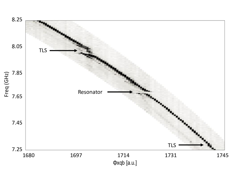
Figure 1: Standard spectroscopy. The arrows indicate avoided level crossings or splittings due to coupling of the qubit to either an engineered on-chip resonant cavity ($7.7GHz$) or random spurious TLS fluctuators.

A typical flux-biased phase qubitSimmonds is composed of an rf SQUID loop with critical current, $I_{q0}$, shunt capacitance, $C_{qs}$, and geometric inductance, $L_{q}$. The phase qubit, described in more detail elsewhereAllman , is coupled to external control and readout circuitry. A dc bias line, coupled to the qubit inductance via a mutual inductance, $M_{qb}$, provides an external flux bias to the qubit. This bias controls the non-linear Josephson inductance of the qubit which controls the energy level spacing between qubit states as well as level anharmonicity. The qubit is operated in a flux bias regime that creates an approximately cubic potential energy well of sufficient anharmonicity to reliably isolate the two lowest metastable energy states for qubit operations. A microwave drive, either capacitively or inductively coupled to the qubit, provides the excitation energy to drive transitions between the two lowest qubit levels, labeled $|{g}\rangle$ and $|{e}\rangle$ respectively. A fast ($\sim 5\,ns$) measure pulse is then applied to induce tunneling of the $|{e}\rangle$ state to the adjacent, stable wellCooper . The state of the qubit is then read out via a dc SQUID coupled to the qubit’s geometric inductance via a mutual inductance, $M_{qs}$. The junctions are $6.5\;\mu{m}^{2}$ via-style junctions with an rf plasma clean used to remove the native oxide barrier before a room temperature thermal oxidation.

In standard spectroscopic measurementsSimmonds , the excited state probability is measured as a function of both drive frequency and applied flux. For a given bias flux, when the applied microwave drive is on resonance with the qubit, the excited state probability peaks. When the qubit transition frequency nears the resonant frequency of a TLS, an avoided crossing occurs, splitting the resonant peak into two peaks (Figure 1). The size of the splitting $S$ is a measure of the coupling strength $hS/2$ between the qubit and the TLS. The smaller the coupling strength, the smaller the splitting size. Long excitation pulse times ($\sim 500\,ns$) and typical qubit linewidths, on the order of $2-10\,MHz$, can limit the ability to resolve the behavior of weakly coupled TLSs.

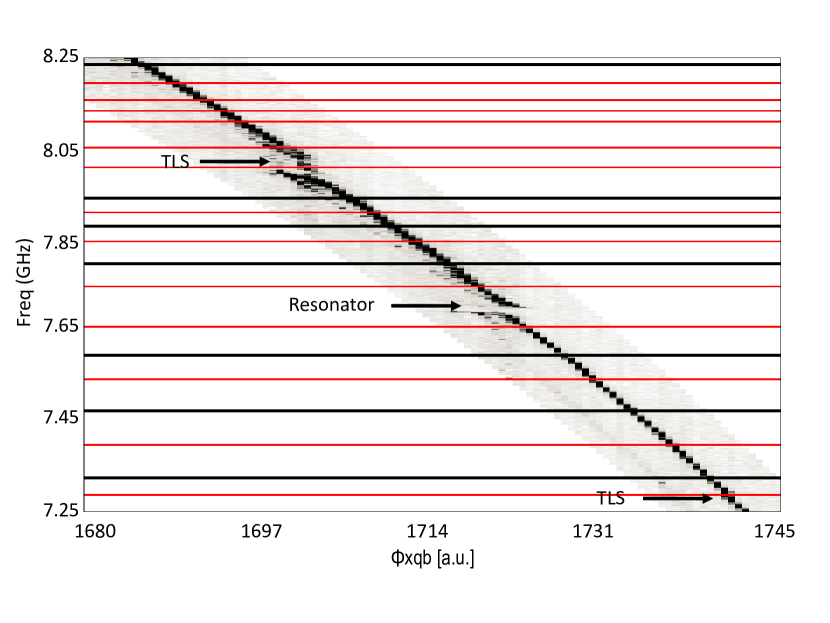
Figure 2: The same spectroscopy from Figure 1 with horizontal red and black lines indicating the qubit frequencies where energy relaxation data (shown in Figure 3) was obtained.

Traditional spectroscopy scans are time-consuming. To achieve a moderately high resolution scan, the step change on the frequency axis is $\Delta{f}\sim{1\,MHz}$. To capture the qubit’s resonance peak with reasonable detail, the total sweep width is typically $\sim{200\,MHz}$. Along the applied flux axis, the resolution is typically on the order of $1/2m\Phi_{0}$ over a range of about $250m\Phi_{0}$. The resulting total number of data points required for a standard qubit spectroscopy is $N_{t}=N_{f}N_{\Phi}\approx{10^{5}}$. The acquisition time per data point, governed by the number of measurements per point as well as the “dead” time associated with the instrument control software is $t_{p}\sim{0.5\,s}$. Thus the time to acquire a basic spectroscopy data set is $t_{spec}=N_{t}t_{p}\approx{15\,hrs}$. Figure 1 shows a typical phase qubit spectroscopy over a range of about $70m\Phi_{0}$ in applied qubit flux. This particular deviceAllman was intentionally strongly coupled to a lumped element resonator as indicated by the avoided crossing at $7.75\,GHz$. The horizontal arrows indicate avoided crossings due to coupling to TLS fluctuators.

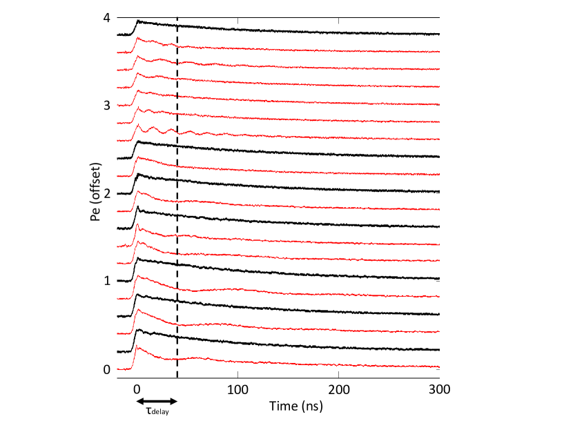
Figure 3: Energy relaxation ($T_{1}$) measurements at particular bias fluxes and frequencies identified in the spectroscopy of Figure 2. The black curves show an exponential dependence as expected. The red curves show coherent oscillations of varying frequency.

Another useful measurement is to determine the energy relaxation time ($T_{1}$) of the qubit. This is done by applying a $\pi$-pulse to the qubit and then sweeping the delay time $\tau_{d}$ between the measure pulse and the end of the $\pi$-pulse. If the qubit is not interacting with another system (other than the environmental bath with many degrees of freedom), the excited state probability decays exponentially in time. If this measurement is performed while the qubit is on resonance with another quantum system, the resultant curve will coherently oscillate with a period proportional to the coupling strength between the qubit and the other system.

In order to obtain a reliable measurement of the qubit’s energy relaxation time, the qubit should be far-detuned from any other coupled systems including TLS fluctuators whose position has previously been determined by visible splittings in the spectroscopic data. According to Figure 1, the energy relaxation curves should be exponential as long as the qubit’s resonant frequency is within a clean region, at least a splitting size away from the center of any splittings.

What we observe is illustrated in Figures 2 and 3. On resonance with any visible splittings, we find coherent oscillations as observed previously with phase qubitsCooper . Remarkably, however, we also find many places within the qubit’s spectral range where the time domain data yields coherent-like oscillations with no evidence of a splitting in the corresponding spectroscopic measurements shown in Figure 2. These oscillations also vary in frequency indicating a random distribution of weak coupling strengths between the TLSs and the qubit as found for larger coupling strengthsMartinisC . The observation of these weakly coupled TLS fluctuators is consistent with predictions based on the standard TLS model for defects in amorphous dielectric solidsMartinisC . The expected distribution of splitting sizes given by Eq. 4 in Ref. MartinisC shows that the defect density scales approximately as $1/S$ where $S$ is the splitting size (in $GHz$) and the coupling strength is given by $hS/2$. Our measurements qualitatively agree with this prediction $-$as the coupling strength decreases, the defect density increases. The measurements recorded in Ref. MartinisC relied on traditional spectroscopic measurements with a minimum splitting resolution of 10 $MHz$.

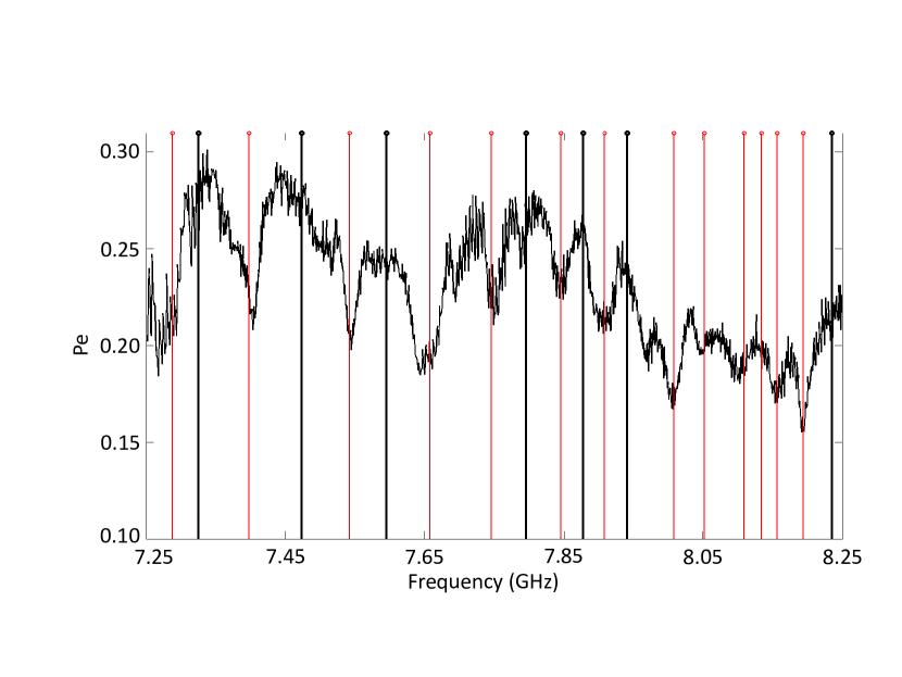
Figure 4: A time-domain dip-scan showing higher spectral TLS density than the standard spectroscopic scan. The peaks correspond to regions in the qubit spectroscopy where the $T_{1}$ decay curve is exponential. The dips correspond to places where a coherent oscillation is present, identifying a TLS fluctuator in the qubit. Note that these dips occur where the standard spectroscopy curve appears to be free from any TLS fluctuators.

We have devised a relatively rapid experimental technique for locating the position of these weakly coupled ($S<10\,MHz$) TLS’s throughout the qubit’s entire spectral range. Once standard spectroscopy has been performed, we have a calibration of the resonant frequency of the qubit as a function of bias flux. We can now search for coherent oscillations at each qubit frequency. Performing high resolution ‘$T_{1}$-scans’ of time domain energy relaxation measurements will certainly reveal the TLS features as coherent oscillations but with data acquisition times that will be as long as standard spectroscopy. In order to reduce the number of data points for a given frequency range of the qubit, we choose a different approach. We hold the measure delay time $\tau_{d}$ fixed at a particular value, just after the maximum excitation of the qubit from the $\pi$-pulse. This value is a small fraction of the energy relaxation time of the qubit, sampling a single point early in the decay with nearly maximum probability. For a given flux, if the qubit is free from interactions with any other systems, the probability amplitude remains high. However, if the qubit is on resonance with a TLS (or any other coherent system), the probability amplitude with undergo oscillations that can produce a ‘dip’ in probability amplitude at the specific sampling point chosen. By taking a single data point for each qubit frequency, we have reduced the required number of points, spanning only the flux dimension, allowing finer resolution ‘dip-scans’ with fewer points and hence shorter acquisition times.

Figure 4 shows a dip-scan with $\tau_{d}=40\,ns$. Here the resolution in applied qubit flux is $\sim 50m\Phi_{0}$ for a total of $1500$ data points with a corresponding acquisition time of approximately $\sim 20$ minutes. Notice that the dips in this scan correspond directly with the TLS fluctuators identified in the full time domain energy relaxation ($T_{1}$) curves shown in Figure 3. It is evident that this technique allows us to count the number of TLS fluctuators with higher resolution than the standard spectroscopy shown in Figure 1.

We have devised a new method for identifying TLS fluctuators in superconducting phase qubits. This ‘dip-scan’ method is general purpose and can be applied to all superconducting qubits with a tunable frequency. This method is useful for future characterizations of Jospehson junction based qubits and may help to elucidate the origin of TLS fluctuators, facilitate their elimination, and eventually lead to increases in superconducting qubit coherence times.

This work was supported by NIST and ARO Grant No. W911NF-06-1-0384.

References

- (1) J. Clarke and F. Wilhelm, Nature 453, 1031 (2008)
- (2) M. Steffen, M. Ansmann, R. Bialczak, N. Katz, E. Lucero, R. McDermott, M. Neeley, E. Weig, A. Cleland, and J. Martinis, Science 313, 1423 (2006)
- (3) R. Simmonds, K. Lang, D. Hite, S. Nam, D. Pappas, and J. Martinis, Physical Review Letters 93, 077003 (2004)
- (4) J. Martinis, K. Cooper, R. McDermott, M. Steffen, M. Ansmann, K. Osborn, K. Cicak, S. Oh, D. Pappas, R. Simmonds, and C. Yu, Physical Review Letters 95, 210503 (2005)
- (5) M. Allman, F. Altomare, J. Whittaker, K. Cicak, D. Li, A. Sirois, J. Strong, J. Teufel, and R. Simmonds, Physical Review Letters, Accepted for publication(2010)
- (6) K. Cooper, M. Steffen, R. McDermott, R. Simmonds, S. Oh, D. Hite, D. Pappas, and J. Martinis, Physical Review Letters 93, 180401 (2004)