Origins of scaling relations in nonequilibrium growth

Abstract

Scaling and hyperscaling laws provide exact relations among critical exponents describing the behavior of a system at criticality. For nonequilibrium growth models with a conserved drift there exist few of them. One such relation is $\alpha+z=4$, found to be inexact in a renormalization group calculation for several classical models in this field. Herein we focus on the two-dimensional case and show that it is possible to construct conserved surface growth equations for which the relation $\alpha+z=4$ is exact in the renormalization group sense. We explain the presence of this scaling law in terms of the existence of geometric principles dominating the dynamics.

I Introduction

One of the great successes of equilibrium statistical mechanics is the classification of critical phenomena into universality classes. These are characterized by sets of critical exponents which describe the system long range physics in the critical point. It is precisely the infrared behavior, which is independent of the microscopic details of the particular system, which lies at the basis of universality.

The numerical values of the critical exponents can be calculated exactly in a number of fortunate cases, otherwise they have to be calculated approximately using some perturbative technique, like notably the renormalization group, or by means of numerical simulations. Scaling and hyperscaling laws provide exact relations among critical exponents and consequently both are a deep expression of the physics and provide a useful calculational tool.

Nonequilibrium statistical mechanics has been built in many situations as an extension of its successful equilibrium counterpart. The classification in terms of universality classes and the tools for computing critical exponents have been adapted to systems out of equilibrium, such as absorbing state transitions henkel and stochastic growth barabasi . This last field is sometimes regarded as paradigmatic within nonequilibrium statistical mechanics. The reason for this is the ubiquity of certain universality classes which were originally discovered in this context and were subsequently found in different areas of physics. A particularly relevant example of this is the Kardar-Parisi-Zhang (KPZ) equation kpz , which scaling behavior has been related to phenomena as diverse as far from equilibrium growth, turbulence and directed polymers.

The KPZ and other nonequilibrium growth equations can be characterized by three scaling exponents: the roughness exponent $\alpha$ characterizing the interface morphology, the dynamic exponent $z$ which specifies the velocity at which correlations propagate and the growth exponent $\beta$ describing its short time dynamics barabasi . One of the most important relations among these exponents is the scaling relation $\alpha=\beta z$, which is fulfilled in a large number of cases. Together with it there exist other scaling and hyperscaling relations describing fundamental characteristics of different physical situations.

This work is devoted to the study of stochastic partial differential equations with a conserved drift. By this we mean that the deterministic part is conservative or, in other words, the spatial average of the deterministic part of the equation vanishes provided suitable boundary conditions are used.

In the following we will examine one of this scaling relations already found in the literature, and we will investigate its possible physical origin. In this work we concentrate on the two-dimensional situation. The paper is organized as follows: in Section II we present some scaling relations for nonequilibrium models, in Section III we give a short geometric derivation of a family of conserved growth equations we will be interested in. Section IV is devoted to the renormalization group analysis of these and other related equations. In the last two Sections we discuss the possible origin of scaling relations for the different models and draw our conclusions.

II Scaling relations

The KPZ equation reads kpz

$$\partial_{t}h=\nu\nabla^{2}h+\frac{\lambda}{2}(\nabla h)^{2}+\xi(\vec{r},t),$$ (1)

where $\xi$ is a zero mean Gaussian noise which correlation is given by $\langle\xi(\vec{r},t)\xi(\vec{r}\,^{\prime},t^{\prime})\rangle=D\delta(\vec{r}-\vec{r}\,^{\prime})\delta(t-t^{\prime})$. If one performs the dilatation $\vec{r}\to b\,\vec{r}$, $t\to b^{z}\,t$ and $h\to b^{\alpha}\,h$ the nonlinearity becomes scale invariant provided $\alpha+z=2$. This scaling relation is actually fulfilled by the KPZ equation in any dimension and its exactness is usually attributed to its Galilean invariance property fns ; medina . However the role of Galilean invariance was put into question in a related nonequilibrium model mccomb ; hochberg ; hochberg2 . In particular, in these works it is shown that neither Galilean invariance nor extended Galilean invariance contribute to vertex non-renormalization beyond the zeroth mode. Also, the same scaling relation $\alpha+z=2$ was found in numerical schemes wio ; wior ; wiop and stochastic equations nicoli ; nicoli2 which do not explicitly fulfill the Galilean invariance symmetry.

Together with the KPZ equation, in this field one finds the Sun-Guo-Grant (SGG) sun and Villain-Lai-Das Sarma (VLDS) villain ; lai equations, which read

$$\partial_{t}h=-\nu\nabla^{4}h+\lambda\nabla^{2}(\nabla h)^{2}+\xi^{(1,2)}(\vec{r},t),$$ (2)

where the noise $\xi^{(1)}$ corresponds to the SGG equation and $\xi^{(2)}$ to the VLDS one.

In both cases the noise is a zero mean stochastic Gaussian process and the respective correlations are:

$$\langle\xi^{(1)}(\vec{r},t)\xi^{(1)}(\vec{r}\,^{\prime},t^{\prime})\rangle=-D\nabla^{2}\delta(\vec{r}-\vec{r}\,^{\prime})\delta(t-t^{\prime}),$$ (3)

and

$$\langle\xi^{(2)}(\vec{r},t)\xi^{(2)}(\vec{r}\,^{\prime},t^{\prime})\rangle=D\delta(\vec{r}-\vec{r}\,^{\prime})\delta(t-t^{\prime}).$$ (4)

For these equations the nonlinearity becomes scale invariant to the dilatation transformation provided the exponents fulfill the scaling relation $\alpha+z=4$. This relation was found to be fulfilled at one loop order renormalization group calculations and it was conjectured to be exact due to the existence of a functional Galilean invariance symmetry sun . However, in janssen , Janssen showed that the mathematics leading to this symmetry was ill-posed. Also, by means of a renormalization group calculation, he showed that this relation does not hold at two loops janssen . The correction to the scaling relation he found is however small and presumably not detectable in simulations or experiments.

We also would like to mention here that this correction has not been found in the results obtained by means of other methods, such that the self-consistent expansion sce1 ; sce2 ; sce3 , when applied to these equations katzav1 . This approximation scheme has proved itself very useful in finding exponent values in some cases in which the renormalization group fails, like for instance for the nonlocal counterpart of some stochastic growth equations katzav2 ; katzav3 . On the other hand, renormalization group analyses have been able to yield exact results for some stochastic growth equations frey1 ; frey2 . We will restrict ourselves to the renormalization group analysis of local equations and leave different approaches for a more comprehensive study. As will be evident in the following, this analysis has a clear interpretation in the cases under consideration.

In the next section we will show that it is possible to find models for which the scaling relation $\alpha+z=4$ is exact to all orders in a renormalization group calculation.

III Geometric derivation of a stochastic growth equation

We now briefly review the geometric derivation of a stochastic growth equation marsili . We concentrate on $d=2$ and assume the following variational approach for the dynamics

$$\frac{\partial h}{\partial t}=\sqrt{1+(\nabla h)^{2}}\left(-\frac{\delta\mathcal{I}}{\delta h}+\xi^{(1,2)}\right),$$ (5)

where we have added the noise term $\xi^{(1,2)}$ and $\mathcal{I}$ is a nonequilibrium potential. We assume it can be expressed as a function of the surface mean curvature only

$$\mathcal{I}=\int f(H)\,\sqrt{1+(\nabla h)^{2}}\,\,d\vec{r},$$ (6)

where $H$ denotes the mean curvature, $f$ is an unknown function of $H$ and whenever we are in two dimensions $\vec{r}=(x,y)$. The presence of the square root terms in Eqs. (5) and (6) describes growth along the normal to the surface.

We will further assume that function $f$ can be expanded in a power series

$$f(H)=K_{0}+K_{1}H+\frac{K_{2}}{2}H^{2}+\cdots,$$ (7)

of which only the zeroth, first, and second order terms will be of relevance at large scales.

The result of the minimization of the potential (6) leads to the equation (see section III.A.3 in marsili )

$$\partial_{t}h=\mu\nabla^{2}h + \lambda\left[(\partial_{xx}h)(\partial_{yy}h)-(\partial_{xy}h)^{2}\right]$$ (8)

$$- \nu\nabla^{4}h+\xi^{(1,2)},$$

to leading order in the small gradient expansion, which assumes $|\nabla h|\ll 1$. Here $\mu=K_{0}$, $\lambda=2K_{1}$ and $\nu=K_{2}$. We note that this equation can be expressed as the divergence of a current $\partial_{t}h=\nabla\cdot j+\xi^{(1,2)}$ for $j=\mu\nabla h+\frac{\lambda}{2}\,\mathrm{cof}(D^{2}h)\cdot\nabla h-\nu\nabla\nabla^{2}h$ provided some regularity conditions on $h$ are assumed muller , and where $\mathrm{cof}(D^{2}h)$ is the cofactor matrix of the Hessian matrix (see Eq. (9) below).

There is another way of finding the first two terms of this equation. The Hessian matrix

$$(D^{2}h)=\left(\begin{array}[]{lr}\partial_{xx}h&\,\partial_{xy}h\\ \partial_{yx}\,h&\,\partial_{yy}h\end{array}\right)$$ (9)

encodes all the information about the convexity and concavity of the interface. This matrix has exactly two tensorial invariants: its trace and its determinant. These are in fact the first two terms of our equation. A related viewpoint was adopted in hanggi in the derivation of a model for amorphous thin film growth.

The term proportional to the Laplacian is associated to the effect of gravity and desorption in the framework of nonequilibrium growth. These effects are negligible in molecular beam epitaxy growth, and this is precisely the context in which the VLDS equation was derived villain ; lai . From a theoretical point of view, the presence of this term in Eq. (8) makes the system evolve towards the linear Edwards-Wilkinson fixed point. So theoretically it is more interesting to neglect this term and this way find a genuine nonlinear dynamics. Setting $\mu=0$ in Eq. (8) yields

$$\partial_{t}h=\lambda\left[(\partial_{xx}h)(\partial_{yy}h)-(\partial_{xy}h)^{2}\right]-\nu\nabla^{4}h+\xi^{(1,2)}.$$ (10)

This equation can be considered as an alternative to both SSG and VLDS equations escudero . Indeed, it is identical to both except for the nonlinearity, that shares the same dimensional analysis properties and the fact that it is conserved.

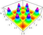
Figure 1: Numerical solution of Eq. (10) in the deterministic limit $D=0$. The values of the parameters are $\lambda=1$ and $\nu=0.1$. We have assumed periodic boundary conditions and the symmetric initial condition $h_{0}=\sin(2\pi x)\sin(2\pi y)$. One sees that holes disappear and mounds form as a consequence of the action of the nonlinearity. Red and orange colors denote negative values of $h$.

In order to clarify the meaning of the nonlinear term in Eq. (10) we numerically solve this equation in the deterministic limit $D=0$, see Fig. 1. We see that holes disappear and mounds form as a consequence of the action of the quadratic nonlinearity. This phenomenology can be explained by means of a simple geometric argument. The surface Gaussian curvature is given in the small gradient limit by $\mathcal{K}\approx h_{xx}h_{yy}-h_{xy}^{2}$, so the dynamics favors the growth of those parts with a positive Gaussian curvature, which is precisely the observed effect.

As a final remark, we note that the growth of perturbations with a defined wavelength may be achieved by means of considering the full Eq. (8) with $\mu<0$. The effect of this type of linear instability on the VLDS equation has already been considered vvedensky . It could be possible to perform a renormalization group analysis in this case as well. One can use the studies on the noisy Kuramoto-Sivashinsky equation which use this technique rodolfo ; hu as a benchmark to this purpose.

IV Renormalization group analysis

Herein we will analyze the equations derived in the previous section as well as some possible variants. Our main tool will be the dynamic renormalization group (RG) as developed in fns ; medina .

IV.1 Methodology

As a first step we will explain how to implement the RG analysis in our current situation. Due to the particular form of the nonlinearity, the present analysis requires considering some subtleties which are not present in the case of more studied nonlinear terms.

We begin with the equation

$$\partial_{t}h=\lambda(h_{xx}h_{yy}-h_{xy}^{2})-\nu\nabla^{4}h+\xi(\vec{r},t),$$ (11)

forced by a white Gaussian noise characterized by its two first moments:

$$\langle\xi(\vec{r},t)\rangle = 0,$$ (12)

$$\langle\xi(\vec{r},t)\xi(\vec{r}\,^{\prime},t^{\prime})\rangle = D\delta(\vec{r}-\vec{r}\,^{\prime})\delta(t-t^{\prime}).$$ (13)

Next we Fourier transform this equation to find

$$h(\vec{k},\omega)=h_{0}(\vec{k},\omega)+\lambda\,G_{0}(\vec{k},\omega)\times$$

$$\int\left[\frac{1}{2}k_{x}^{2}q_{y}^{2}+\frac{1}{2}k_{y}^{2}q_{x}^{2}-k_{x}k_{y}q_{x}q_{y}\right]$$

$$\times\,h(\vec{k}-\vec{q},\omega-\Omega)\,h(\vec{q},\Omega)\,\frac{d\Omega\,d\vec{q}}{(2\pi)^{3}},$$ (14)

where

$$h_{0}(\vec{k},\omega)=G_{0}(\vec{k},\omega)\,\tilde{\xi}(\vec{k},\omega),$$ (15)

$$G_{0}(\vec{k},\omega)=(-i\omega+\nu k^{4})^{-1},$$ (16)

$\tilde{\xi}$ is the Fourier transformed white noise, $k=|\vec{k}|$ and $\vec{k}=(k_{x},k_{y})$ (the same holds for $\vec{q}$). This equation is to be solved iteratively in the vertex. The resulting Feynman diagrams are identical to the ones represented in medina and sun . The dynamic renormalization group technique fns calculates the intermediate values of the renormalized parameters by integrating out fast modes in the momentum shell $e^{-\ell}\Lambda\leq k\leq\Lambda$, where $\Lambda$ is the momentum cutoff and $\ell$ parameterizes the change across different scales. The remaining slow modes ($k<\Lambda$) are restored to full momentum space by means of rescaling space and time $\vec{k}\,^{\prime}=e^{-\ell}\,\vec{k}$, $\omega^{\prime}=e^{-z\,\ell}\,\omega$, and field $h^{\prime}=e^{\alpha\,\ell}\,h$. The scaled field $h^{\prime}$ obeys Eq. (14) as well provided the renormalized coefficients satisfy the renormalization group flow equations, that we will calculate in the following.

In the present case the noise amplitude is $D$, the propagator is

$$\frac{1}{-i\omega+\nu k^{4}},$$ (17)

and the vertex is

$$\lambda\int\left(\frac{1}{2}k_{x}^{2}q_{y}^{2}+\frac{1}{2}k_{y}^{2}q_{x}^{2}-k_{x}k_{y}q_{x}q_{y}\right)=\lambda\int\frac{1}{2}\left(\vec{k}\cdot\vec{q}\,^{\perp}\right)^{2},$$ (18)

where $\vec{q}\,^{\perp}=(q_{y},-q_{x})$. The last equality is advantageous because it will allow us to integrate over the angle formed by $\vec{k}$ and $\vec{q}\,^{\perp}$. If this equality were not present we would have to carry out a more complicated calculation reminiscent to that described in the Appendix. Note that here we are explicitly using we are in $d=2$. In two dimensions the situation is particularly simple because for any given non-zero vector there are just two vectors of a given modulus perpendicular to it. Our selection is arbitrary: choosing the opposite possibility for $\vec{q}\,^{\perp}$ does not modify the result as the scalar product on the right hand side of Eq. (18) is squared. Designing the optimal vertex form for a similar model built in $d>2$ is a more technical issue.

The first diagrammatic contribution to propagator renormalization is

$$\frac{\lambda^{2}}{8\pi^{3}}\frac{1}{(-i\omega+\nu k^{4})^{2}}\int\left[\frac{1}{2}(k_{x}-q_{x})^{2}q_{y}^{2}+\frac{1}{2}(k_{y}-q_{y})^{2}q_{x}^{2}-(k_{x}-q_{x})(k_{y}-q_{y})q_{x}q_{y}\right]\times$$

$$\left(\frac{1}{2}k_{x}^{2}q_{y}^{2}+\frac{1}{2}k_{y}^{2}q_{x}^{2}-k_{x}k_{y}q_{x}q_{y}\right)\frac{1}{-i\Omega+\nu q^{4}}\frac{1}{i\Omega+\nu q^{4}}\frac{D}{-i(\omega-\Omega)+\nu|\vec{k}-\vec{q}|^{4}}\,d\vec{q}\,\,d\Omega.$$ (19)

It is important to realize that we have the simplification

$$\frac{1}{2}(k_{x}-q_{x})^{2}q_{y}^{2}+\frac{1}{2}(k_{y}-q_{y})^{2}q_{x}^{2}-(k_{x}-q_{x})(k_{y}-q_{y})q_{x}q_{y}=\frac{1}{2}k_{x}^{2}q_{y}^{2}+\frac{1}{2}k_{y}^{2}q_{x}^{2}-k_{x}k_{y}q_{x}q_{y}.$$ (20)

Now using Eq. (18) we reduce this diagrammatic contribution to

$$\frac{\lambda^{2}}{32\pi^{3}}\frac{D}{\nu^{2}k^{8}}\int\frac{k^{4}q^{4}\cos^{4}(\theta)}{(-i\Omega+\nu q^{4})(i\Omega+\nu q^{4})^{2}}q\,dq\,d\theta,$$ (21)

where $\theta$ is the angle formed by $\vec{k}$ and $\vec{q}\,^{\perp}$, and we have carried out the limit $k,\omega\to 0$. We note this contribution is relevant because the integrand is $O(k^{4})$ and the propagator renormalizes at this same order. Diagrammatically this one loop order is identical to the one represented, for instance, in figure 2(a) in medina and figure 1(b) in sun .

The first diagrammatic contribution to noise renormalization is

$$\frac{1}{8\pi^{3}}\frac{\lambda^{2}}{\nu^{2}k^{8}}\int\frac{D^{2}}{(\nu^{2}q^{8}+\Omega^{2})^{2}}\left(\frac{1}{2}k_{x}^{2}q_{y}^{2}+\frac{1}{2}k_{y}^{2}q_{x}^{2}-k_{x}k_{y}q_{x}q_{y}\right)^{2}\,d\vec{q}\,\,d\Omega,$$ (22)

in the limit $k,\omega\to 0$. This contribution is irrelevant because the integrand is $O(k^{4})$. The corresponding diagrams at one loop are the same as those represented, for instance, in figure 2(b) in medina and figure 1(c) in sun .

The first diagrammatic contribution to vertex renormalization is irrelevant for exactly the same reason. Diagrammatically this one loop order is identical to the one represented, for instance, in figure 2(c) in medina and figure 1(d) in sun . In this case all diagrams have three external legs: one corresponds to an ongoing $\vec{k}_{1}$ momentum and the other two to outgoing $\vec{k}_{2}$ and $\vec{k}_{1}-\vec{k}_{2}$ momenta. Consider for instance the intermediate vertex corresponding to an ongoing leg $\vec{k}_{1}$ and two outgoing legs $\vec{q}$ and $\vec{k}_{1}-\vec{q}$:

$$\frac{1}{2}(k_{1x}-q_{x})^{2}q_{y}^{2}+\frac{1}{2}(k_{1y}-q_{y})^{2}q_{x}^{2}-(k_{1x}-q_{x})(k_{1y}-q_{y})q_{x}q_{y}$$ (23)

which is of order $O(k^{2})$. The other two intermediate vertices are trivially of order $O(k^{2})$, so the order of this diagrammatic contribution is $O(k^{6})$. Automatically this implies this contribution is irrelevant in the hydrodynamic limit $k\to 0$, because the vertex renormalizes at order $O(k^{4})$.

The renormalization group flow equations then read

$$\frac{d\nu}{d\ell} = \nu\left[z-4-\frac{3}{64\pi}\frac{\lambda^{2}D}{\nu^{3}}\right],$$ (24)

$$\frac{dD}{d\ell} = D\left[z-2-2\alpha\right],$$ (25)

$$\frac{d\lambda}{d\ell} = \lambda\left[z+\alpha-4\right].$$ (26)

These equations yield the following values of the critical exponents: $\alpha=2/3$ and $z=10/3$. The exponents are exactly the ones found for the VLDS equation at one loop order. The difference in this case is that the result is exact. We note that noise does not renormalize at any order in the loop expansion yielding the exactness of Eq. (25). This is a well known fact due to the conserved character of the drift of the stochastic growth equation. In the present case, Eq. (26) is exact too due to the fact that the vertex does not renormalize at any order in the loop expansion. All diagrams contributing to vertex renormalization at any order are irrelevant in exactly the same way we have shown herein for the one loop order diagrams.

As we have seen, the exactness of the scaling relation $\alpha+z=4$ holds in this case. The current situation is genuinely different from the one concerning both SGG and VLDS equations. In that case vertex non-renormalization was fulfilled at one loop due to the cancellation of all diagrams contributing at this order. Janssen showed that the cancellation of diagrams contributing to vertex renormalization at two loops is not exact, what leads to the inexactness of the scaling relation janssen . In the present case this argument does not apply because there is no cancellation of diagrams: instead all diagrams contributing to vertex renormalization are irrelevant. So the reason underlying the exactness of the scaling relation is fundamentally different.

It is important to note we have used a symmetrized vertex given by Eq. (18) after using the simplification Eq. (20). This choice is by no means unique, as we could have chosen a different vertex form, such as

$$\lambda\int\left[(k_{x}-q_{x})^{2}q_{y}^{2}-(k_{x}-q_{x})(k_{y}-q_{y})q_{x}q_{y}\right],$$ (27)

or an infinite number of different possibilities. Among all of them, the only one which is symmetric under a simultaneous change of coordinates $(k_{x}\longleftrightarrow k_{y},q_{x}\longleftrightarrow q_{y})$ is Eq. (18). Contrary to what we have shown herein, using an asymmetric form results in the dependence of the RG flow equations on the polar angle in Fourier space $\phi$. Indeed, the substitution $k_{x}=k\,\cos(\phi)$ and $k_{y}=k\,\sin(\phi)$ in Eq. (27) does not lead to a vertex form independent of $\phi$. Formally proceeding, this dependence is translated to the flow equations. This leads to a perfectly valid result whenever the resulting exponents are independent of this angle, see escudero . However, in the general case, some dependence on this angle may arise. The presence of this angle in the RG flow equations signals the generation of an integral operator in the stochastic growth equation when its coefficients become renormalized. This consequently leads to a more complicated mathematical treatment, as it implies the necessity of restarting the RG procedure including the newly generated operators. In order to avoid this, the symmetric form Eq. (18) must be used. We discuss in Appendix A the different results which may arise from the RG analysis employing asymmetric vertex forms.

IV.2 Results for different models

Now we will explore different stochastic growth equations with the methodology explained in the previous section. Our goal is getting a deeper understanding of the properties of the nonlinearity we have considered so far or variants of it. In particular, we will show that vertex non-renormalization is present in those cases in which noise renormalization is present.

We start with a variation of Eq. (11)

$$\partial_{t}h=\lambda(h_{xx}h_{yy}-h_{xy}^{2})-\nu\nabla^{4}h+\xi(\vec{r},t),$$ (28)

where now the noise is conserved, i. e. it is white and Gaussian and its two first moments are given by

$$\langle\xi(\vec{r},t)\rangle = 0,$$ (29)

$$\langle\xi(\vec{r},t)\xi(\vec{r}\,^{\prime},t^{\prime})\rangle = -D\nabla^{2}\delta(\vec{r}-\vec{r}\,^{\prime})\delta(t-t^{\prime}).$$ (30)

As we have already outlined, this equation can be considered as an analogue of the SSG one. The renormalization group flow equations can be obtained following analogous arguments to those of the previous section and read

$$\frac{d\nu}{d\ell} = \nu\left[z-4-\frac{3}{64\pi}\frac{\lambda^{2}D}{\nu^{3}}\right],$$ (31)

$$\frac{dD}{d\ell} = D\left[z-4-2\alpha\right],$$ (32)

$$\frac{d\lambda}{d\ell} = \lambda\left[z+\alpha-4\right].$$ (33)

From here we get the critical exponents $\alpha=0$ and $z=4$, this is, the SSG universality class. We emphasize that the last two RG flow equations are exact, i. e. both noise and vertex do not renormalize at any order in the loop expansion, for exactly the same reasons as in the previous section.

As the next example we consider the following equation

$$\partial_{t}h=\lambda(h_{xx}h_{yy}-h_{xy}^{2})+\nu\nabla^{6}h+\xi(\vec{r},t),$$ (34)

where the noise is again white and Gaussian and its first and second moments are given by Eqs. (29) and (30) respectively. We note that the sixth order differential operator has already been deduced in the context of nonequilibrium growth from atomistic models vvedensky2 . The renormalization group flow equations become

$$\frac{d\nu}{d\ell} = \nu\left[z-6-\frac{45}{128\pi}\frac{\lambda^{2}D}{\nu^{3}}\right],$$ (35)

$$\frac{dD}{d\ell} = D\left[z-4-2\alpha\right],$$ (36)

$$\frac{d\lambda}{d\ell} = \lambda\left[z+\alpha-4\right].$$ (37)

We find again the same exponents $\alpha=0$ and $z=4$ due to noise and vertex non-renormalization (both results are exact again).

The next equation that deserves our attention is a different variation of Eq. (11)

$$\partial_{t}h=\lambda(h_{xx}h_{yy}-h_{xy}^{2})-\nu\nabla^{4}h+\xi(\vec{r},t),$$ (38)

where the noise is as always white and Gaussian but this time its mean and correlation are

$$\langle\xi(\vec{r},t)\rangle = 0,$$ (39)

$$\langle\xi(\vec{r},t)\xi(\vec{r}\,^{\prime},t^{\prime})\rangle = D\nabla^{4}\delta(\vec{r}-\vec{r}\,^{\prime})\delta(t-t^{\prime}).$$ (40)

This sort of higher order contribution to conserved noise has been previously considered in the literature tang . In this case, a simple dimensional analysis shows that the nonlinearity is not relevant and leads to the exponents $\alpha=-1$ and $z=4$. In this context a negative exponent $\alpha$ is identified with a flat interface.

In the case of Eq. (34)

$$\partial_{t}h=\lambda(h_{xx}h_{yy}-h_{xy}^{2})+\nu\nabla^{6}h+\xi(\vec{r},t),$$ (41)

where the noise is white and Gaussian and its mean and correlation are given by Eqs. (39) and (40) respectively, the RG analysis yields a negative exponent $\alpha$ as well. This can be read from the following RG flow equations:

$$\frac{d\nu}{d\ell} = \nu\left[z-6+\frac{45}{128\pi}\frac{\lambda^{2}D}{\nu^{3}}\right],$$ (42)

$$\frac{dD}{d\ell} = D\left[z-6-2\alpha+\frac{3}{512\pi}\frac{\lambda^{2}D}{\nu^{3}}\right],$$ (43)

$$\frac{d\lambda}{d\ell} = \lambda\left[z+\alpha-4\right].$$ (44)

Thus the exponents become $\alpha=240/179-2\approx-0.66$ and $z=6-240/179\approx 4.66$. Note that vertex non-renormalization is again present and exact, while the noise is renormalized at one loop order. This result, noise renormalization in a conserved model, was already found in the literature for this kind of noise and a different drift tang .

Now we direct our analysis to higher order equations like

$$\partial_{t}h=\lambda(h_{xx}h_{yy}-h_{xy}^{2})-\nu\nabla^{8}h+\xi(\vec{r},t),$$ (45)

where the noise is white and Gaussian with mean and correlation given by Eqs. (29) and (30). The eighth order differential operator can be considered as a higher order diffusion mechanism in the context of nonequilibrium growth, when we regard continuum equations as hydrodynamic descriptions of atomistic models vvedensky2 . This equation can be analyzed with the RG technique and we have found that neither noise nor vertex do renormalize at any order, what yields the exact exponents $\alpha=0$ and $z=4$.

The previous equation

$$\partial_{t}h=\lambda(h_{xx}h_{yy}-h_{xy}^{2})-\nu\nabla^{8}h+\xi(\vec{r},t),$$ (46)

can be studied with a Gaussian white noise having as first moments Eqs. (39) and (40). Its analysis by means of the RG method yields a negative value of exponent $\alpha$. In this case the flow equations read

$$\frac{d\nu}{d\ell} = \nu\left[z-8+\frac{1}{\pi}\frac{\lambda^{2}D}{\nu^{3}}\right],$$ (47)

$$\frac{dD}{d\ell} = D\left[z-6-2\alpha+\frac{3}{128\pi}\frac{\lambda^{2}D}{\nu^{3}}\right],$$ (48)

$$\frac{d\lambda}{d\ell} = \lambda\left[z+\alpha-4\right],$$ (49)

yielding the exponents $z=1768/381\approx 4.64$ and $\alpha=4-z\approx-0.64$. Again we find that vertex non-renormalization is exact and noise renormalizes at one loop order.

Our last example is the following equation

$$\partial_{t}h=\lambda\nabla^{4}(h_{xx}h_{yy}-h_{xy}^{2})-\nu\nabla^{8}h+\xi(\vec{r},t),$$ (50)

where the white and Gaussian noise is characterized by the moments Eq. (39) and (40). We found this stochastic differential equation specially interesting because its RG analysis is meaningless as neither propagator, nor noise, nor vertex renormalize at any order in this case. So a different technique should be employed for this kind of model. One possibility would be the use of self-consistent expansions sce1 ; sce2 ; sce3 ; katzav1 ; katzav2 ; katzav3 as we mentioned in the Introduction, but we have not explored this possibility yet. We also note that, due to the high order of differentiation in every term of this equation, its numerical analysis should be a hard task too.

V Origins of scaling

We now examine the physical origin of scaling relations. The exactness of the relation $\alpha+z=4$ in all our equations can be traced back to expansion (7). Higher order terms are meant to describe smaller scale physics. Accordingly, the exactness of this scaling relation indicates that the nonlinearity totally dominates over surface diffusion in the large scale. Considering the full Eq. (8) with $\mu>0$ we find, in agreement with Eq. (7), that the Laplacian dominates. So expansion (7) provides a simple geometric interpretation of the renormalization group results and the exactness of this scaling relation.

The exactness of the exponents for the SSG and VLDS universality classes, found in our equations, was due to noise and vertex non-renormalization. Noise non-renormalization is a common fact, and its origin is in the conserved character of the drift, which has been shown in previous works sun ; lai ; janssen . The case of the vertex is new. Indeed, the vertex structure

$$\lambda\int\frac{1}{2}\left(\vec{k}\cdot\vec{q}^{\perp}\right)^{2}$$ (51)

implies that all contributions to the renormalization of the vertex are $O(k^{6})$, while the vertex renormalizes at $O(k^{4})$. The concrete calculations have been carried out in Sec. IV.1. In other words, the vertex is not renormalized because all the generated Feynman diagrams correspond to irrelevant contributions. This is easily seen by noting that in the renormalization group calculation the vertex contributions result from integrating against measure (51). The procedure is identical to the one carried out for the KPZ equation medina mutatis mutandis. Any possible contributions to the renormalized coefficients come from integrands that are exactly $O(k^{0})$, as higher order contributions are irrelevant. It is immediate realizing that the $O(k^{0})$ contribution of measure (51) is identically zero. In consequence, noise and vertex do not renormalize at any order in the loop expansion. This is in contrast to what happened to the SGG and VLDS equations, for which the vertex one loop diagrams were relevant but they cancelled each other out sun ; lai .

While the renormalization group is a perturbative technique which may allow access to the critical exponents, it is also possible to unveil (at least part of) the critical behavior by means of finding the stationary probability distribution of a given Langevin equation. This approach has being successfully exploited in the past katzav4 ; katzav5 ; kardar , mainly (but not only kardar ) in those cases in which the stationary state is Gaussian. In our case it is possible as well, as was shown in escudero , to formally find the exact stationary probability density corresponding to Eq. (11) using its gradient flow structure

$$\partial_{t}h=-\frac{\delta\mathcal{V}}{\delta h}+\xi(\vec{r},t),\qquad\mathcal{V}[h]=-\int\left[\lambda\,h_{x}h_{y}h_{xy}-\frac{\nu}{2}(\nabla^{2}h)^{2}\right]dx\,dy.$$ (52)

Then the probability density reads

$$\mathcal{P}\sim\exp\left\{\int\left[\lambda\,h_{x}h_{y}h_{xy}-\frac{\nu}{2}(\nabla^{2}h)^{2}\right]dx\,dy\right\},$$ (53)

and it is evidently not Gaussian. This distribution is of course not normalizable due to the presence of the cubic term, and consequently this expression is purely formal. Its form suggests that the interface profile could be initially dominated by the quadratic term, and after some transient the noise could drive the interface out of this potential well. Then for long times the cubic term would dominate, as the dynamics would be separated from the initial Gaussian behavior by the nonlinearity. This simple picture, derived from the formal stationary probability distribution, agrees with the results of the renormalization group analysis.

VI Conclusions

In this work we have shown that the scaling relation $\alpha+z=4$, which originates in the vertex non-renormalization and which is inexact in the renormalization group sense for both SSG and VLDS equations, becomes exact in the case of Eq. (10) with both conserved and non-conserved noises. The physical origin of this scaling relation is not the existence of a symmetry (such as a functional Galilean invariance) but the existence of the geometric principle described by Eqs. (5)-(6)-(7).

We have proven the exactness of this scaling relation in $d=2$, in the renormalization group sense, for a series of stochastic differential equations presented in Sec. IV.2. Therein we have found that vertex non-renormalization is exact for the considered nonlinearity independently of whether noise is renormalized or not. The validity of these results extends to all examined models, except the last one. In that case, the higher order of differentiation precludes the access to the critical behavior by means of the employment of the RG technique, as we have shown.

We have focused on conserved surface growth but the existence of scaling laws happens as well in non-conserved cases. Notably the KPZ equation obeys the relation $\alpha+z=2$. Although this scaling relation has been traditionally attributed to the existence of a Galilean invariance in the equation, recent numerical work suggests that it is possible to find discrete schemes which do not obey this symmetry and are still able to reproduce the KPZ universality class wio ; wior ; wiop . Perhaps the existence of a geometric principle, akin to the one discussed here, could be a possible alternative explanation. The origin of such a principle is not clear so far, but the variational formulation of the KPZ equation wio2 might have some relation with it, in case it exists.

Appendix A RG Analysis with an asymmetric vertex form

As mentioned in section IV.1 using asymmetric vertex forms leads to the explicit appearance of the polar angle in Fourier space. This fact signals the generation of new operators and requires the employment of a more sophisticated mathematical treatment that will be outlined at the end of this appendix. The aim of this appendix is showing that, nevertheless, it is possible to formally proceed with the calculations ignoring the presence of this angle and still find the good result. Sometimes this is possible, sometimes it is not. Herein we exemplify these different possibilities.

We consider the equation

$$\partial_{t}h=\lambda(h_{xx}h_{yy}-h_{xy}^{2})-\nu\nabla^{4}h+\xi^{(1,2)}.$$ (54)

First of all we shall concentrate on the non-conserved noise case $\xi=\xi^{(2)}$. We employ the following asymmetric vertex form

$$h(\vec{k},\omega)=h_{0}(\vec{k},\omega)+\lambda\,G_{0}(\vec{k},\omega)\times$$

$$\int\left[(k_{x}-q_{x})^{2}q_{y}^{2}-(k_{x}-q_{x})(k_{y}-q_{y})\,q_{x}\,q_{y}\right]$$

$$\times\,h(\vec{k}-\vec{q},\omega-\Omega)\,h(\vec{q},\Omega)\,\frac{d\Omega\,d\vec{q}}{(2\pi)^{3}},$$ (55)

where

$$h_{0}(\vec{k},\omega)=G_{0}(\vec{k},\omega)\,\tilde{\xi}(\vec{k},\omega),$$ (56)

$$G_{0}(\vec{k},\omega)=(-i\omega+\nu k^{4})^{-1},$$ (57)

$\tilde{\xi}$ is the Fourier transformed white noise, $k=|\vec{k}|$ and $\vec{k}=(k_{x},k_{y})$ (the same holds for $\vec{q}$). The renormalized coefficients satisfy the RG flow equations, which at one loop order are given by

$$\frac{d\nu}{d\ell} = \nu\left[z-4-\frac{\lambda^{2}D}{8\pi\nu^{3}}\cos^{2}(\phi)\right],$$ (58)

$$\frac{dD}{d\ell} = D\left[z-2-2\alpha\right],$$ (59)

$$\frac{d\lambda}{d\ell} = \lambda\left[z+\alpha-4\right].$$ (60)

The variable $\phi$ is the polar angle in Fourier space. An alternative way of thinking about this angle is through the relation

$$\cos^{2}(\phi)=\frac{\widehat{h_{xx}}}{\widehat{h_{xx}}+\widehat{h_{yy}}},$$ (61)

where $\hat{\cdot}$ denotes the spatial Fourier transform. The values of the exponents are independent of this angle and take the correct values $\alpha=2/3$ and $z=10/3$.

Now we move to the case of conserved noise, i. e. to the model

$$\partial_{t}h=\lambda(h_{xx}h_{yy}-h_{xy}^{2})-\nu\nabla^{4}h+\xi^{(1)}.$$ (62)

Repeating the dynamic renormalization group calculations we arrive at the flow equations for the effective parameters

$$\frac{d\nu}{d\ell} = \nu\left[z-4-\frac{\lambda^{2}D}{8\pi\nu^{3}}\cos^{2}(\phi)\right],$$ (63)

$$\frac{dD}{d\ell} = D\left[z-4-2\alpha+\frac{D\lambda^{2}}{64\pi\nu^{3}}\right],$$ (64)

$$\frac{d\lambda}{d\ell} = \lambda\left[z+\alpha-4\right].$$ (65)

The resulting exponents are independent of $\phi$ and consequently they are the correct ones: $\alpha=0$ and $z=4$. Note however that the noise renormalization that arises in this case should be interpreted as a spurious result since it does not appear in the case of a symmetric vertex form, cf. Eqs (31)-(32)-(33).

Now we move to the last model

$$\partial_{t}h=\lambda(h_{xx}h_{yy}-h_{xy}^{2})+\nu\nabla^{6}h+\xi^{(1)}.$$ (66)

The renormalization group leads us this time to the flow equations

$$\frac{d\nu}{d\ell} =$$

$$= \nu\left[z-6+\frac{\lambda^{2}D}{256\pi\nu^{3}}\cos^{2}(\phi)\{19-10\cos(2\phi)\}\right],$$

$$\frac{dD}{d\ell} = D\left[z-4-2\alpha+\frac{D\lambda^{2}}{64\pi\nu^{3}}\right],$$ (68)

$$\frac{d\lambda}{d\ell} = \lambda\left[z+\alpha-4\right].$$ (69)

So we find the $\phi-$dependent exponents

$$\alpha = \frac{8}{-4+3\cos^{2}(\phi)\{19-10\cos(2\phi)\}},$$ (70)

$$z = 4+\frac{8}{4-3\cos^{2}(\phi)\{19-10\cos(2\phi)\}}.$$ (71)

In this case these values have to be considered invalid because it is not possible to recover the correct exponents found in the analysis performed with the symmetric vertex form from Eqs. (70, 71). Indeed, averaging $\phi$ out from either Eqs. (A, 68, 69) or (70, 71) does not reproduce the actual values of the exponents $\alpha=0$ and $z=4$ known form Eqs. (35, 36, 37). The correct way to proceed now would be deriving the stochastic growth equation with renormalized coefficients. This leads to the appearance of new operators in the equation. An example with a fourth order equation can be found in sarma . In this example, contrary to ours, a new term in the equation is generated; in our present case the differential operators become integro-differential. In fact, $\cos^{2}(\phi)$ gives rise to a linear integral operator which in Fourier space reduces itself to a multiplication by the factor

$$\frac{k_{x}^{2}}{k_{x}^{2}+k_{y}^{2}}$$ (72)

of the field over which it is applied stein . The resulting stochastic growth equation should be analyzed again by means of the RG technique. Obviously, this is much harder than using a symmetric vertex form.

In summary, it is possible to analyze stochastic growth equations using asymmetric vertex forms. One can formally proceed, ignore the presence of polar angles in Fourier space, and end up with $\phi-$dependent flow equations. If the resulting exponents are independent of these angles one can conclude the calculation. If there is $\phi$ dependence in the exponents, then one has to derive the equation with the newly generated operators and restart the analysis. The overall procedure is more complicated than using a symmetric vertex form.

References

- (1) M. Henkel, H. Hinrichsen, and S. Lübeck, Non-Equilibrium Phase Transitions, Volume I: Absorbing Phase Transitions (Springer, Dordrecht, 2008).
- (2) A.-L. Barabási and H. E. Stanley, Fractal Concepts in Surface Growth (Cambridge University Press, Cambridge, 1995).
- (3) M. Kardar, G. Parisi, and Y.-C. Zhang, Phys. Rev. Lett. 56, 889 (1986).
- (4) D. Forster, D. R. Nelson, and M. J. Stephen, Phys. Rev. A 16, 732 (1977).
- (5) E. Medina, T. Hwa, M. Kardar, and Y.-C. Zhang, Phys. Rev. A 39, 3053 (1989).
- (6) W. D. McComb, Phys. Rev. E 71, 037301 (2005).
- (7) A. Berera and D. Hochberg, Phys. Rev. Lett. 99, 254501 (2007).
- (8) A. Berera and D. Hochberg, Nucl. Phys. B 814, 522 (2009).
- (9) H. S. Wio, J. A. Revelli, R. R. Deza, C. Escudero, and M. S. de la Lama, EPL 89, 40008 (2010).
- (10) H. S. Wio, J. A. Revelli, R. R. Deza, C. Escudero, and M. S. de la Lama, Phys. Rev. E 81, 066706 (2010).
- (11) H. S. Wio, C. Escudero, J. A. Revelli, R. R. Deza, and M. S. de la Lama, Philos. T. R. Soc. A 369, 396 (2011).
- (12) M. Nicoli, R. Cuerno, and M. Castro, Phys. Rev. Lett. 102, 256102 (2009).
- (13) M. Nicoli, R. Cuerno, and M. Castro, arXiv:1110.0431.
- (14) T. Sun, H. Guo, and M. Grant, Phys. Rev. A 40, 6763 (1989).
- (15) J. Villain, J. Phys. I (France) 1, 19 (1991).
- (16) Z.-W. Lai and S. Das Sarma, Phys. Rev. Lett. 66, 2348 (1991).
- (17) H. K. Janssen, Phys. Rev. Lett. 78, 1082 (1997).
- (18) M. Schwartz and S. F. Edwards, Europhys. Lett. 20, 301 (1992).
- (19) M. Schwartz and S. F. Edwards, Phys. Rev. E 57, 5730 (1998).
- (20) E. Katzav and M. Schwartz, Phys. Rev. E 60, 5677 (1999).
- (21) E. Katzav, Phys. Rev. E 65, 32103 (2002).
- (22) E. Katzav, Phys. Rev. E 68, 46113 (2003).
- (23) E. Katzav, Eur. Phys. J. B 54, 137(R) (2006).
- (24) H. K. Janssen, U. C. Täuber, and E. Frey, Eur. Phys. J. B 9, 491 (1999).
- (25) E. Frey, U. C. Täuber, and H. K. Janssen, Europhys. Lett. 47, 14 (1999).
- (26) M. Marsili, A. Maritan, F. Toigo, and J. R. Banavar, Rev. Mod. Phys. 68, 963 (1996).
- (27) S. Müller, C. R. Acad. Sci. Paris, Sér. I Math. 311, 13 (1990).
- (28) M. Raible, S. G. Mayr, S. J. Linz, M. Moske, P. Hänggi, and K. Samwer, Europhys. Lett. 50, 61 (2000).
- (29) C. Escudero, Phys. Rev. Lett. 101, 196102 (2008).
- (30) C. A. Haselwandter and D. D. Vvedensky, Phys. Rev. Lett. 98, 046102 (2007).
- (31) R. Cuerno and K. B. Lauritsen, Phys. Rev. E 52, 4853 (1995).
- (32) L. Zhang, G. Tang, Z. Xun, K. Han, H. Chen, and B. Hu, Eur. Phys. J. B 63, 227 (2008).
- (33) C. A. Haselwandter and D. D. Vvedensky, Phys. Rev. B 74, 121408(R) (2006).
- (34) L.-H. Tang and T. Nattermann, Phys. Rev. Lett. 66, 2899 (1991).
- (35) E. Katzav, Physica A 308, 25 (2002).
- (36) E. Katzav, Physica A 309, 79 (2002).
- (37) R. A. da Silveira and M. Kardar, Phys. Rev. E 68, 046108 (2003).
- (38) H. S. Wio, Int. J. Bif. Chaos 19, 2813 (2009).
- (39) S. Das Sarma and R. Kotlyar, Phys. Rev. E 50, R4275 (1994).
- (40) This operator is related to the Riesz transform, see E. M. Stein, Harmonic Analysis: Real-Variable Methods, Orthogonality and Oscillatory Integrals (Princeton University Press, Princeton, New Jersey, 1993).