on leave from ITEP, Moscow, Russia.
Phase diagram of hot QCD in an external magnetic field:
possible splitting of deconfinement and chiral transitions
Abstract
The structure of the phase diagram for strong interactions becomes richer in the presence of a magnetic background, which enters as a new control parameter for the thermodynamics. Motivated by the relevance of this physical setting for current and future high-energy heavy ion collision experiments and for the cosmological QCD transitions, we use the linear sigma model coupled to quarks and to Polyakov loops as an effective theory to investigate how the chiral and the deconfining transitions are affected, and present a general picture for the temperature–magnetic field phase diagram. We compute and discuss each contribution to the effective potential for the approximate order parameters, and uncover new phenomena such as the paramagnetically-induced breaking of global symmetry, and possible splitting of deconfinement and chiral transitions in a strong magnetic field.
pacs:
11.10.Wx; 12.38.Mh; 25.75.Nq; 11.30.RdI Introduction
The phase diagram of QCD has a very rich structure, and keeps unveiling new, sometimes unexpected phases of strong interactions as one plays with thermodynamic control parameters such as the temperature, chemical potentials and quark masses (for recent results, see e.g. Ref. CPOD2009 ). A particular external control parameter that is often overlooked, however, is the magnetic field. Since quarks and charged hadrons couple to the magnetic field and neutral hadrons do not, this control parameter can affect the phase structure of QCD in a nontrivial fashion. Moreover, it is present in most physical systems exhibiting deconfinement and chiral symmetry restoration. The example that was considered to be the most spectacular is from astrophysics, provided by magnetars magnetars . Besides, magnetic fields are expected to be strong and play an important role in structure formation in the early universe, during the epochs of the electroweak and the QCD primordial phase transitions Schwarz:2003du . However, it was recently found that non-central high-energy heavy ion collisions might generate the most intense observed magnetic fields, much stronger than in magnetars, reaching values of Gauss, which corresponds to , where is the fundamental charge and is the pion mass. These magnetic fields are short-lived for very high energies but play an important role in possible experimental signatures of strong CP violation and the phenomenon of the chiral magnetic effect Kharzeev:1998kz ; Kharzeev:2007jp ; Skokov:2009qp ; Fukushima:2010fe .
In this paper we present a general picture for the temperature–magnetic field phase diagram of QCD, restricting our analysis to a vanishing baryonic chemical potential. In particular, we investigate how the chiral and the deconfining transitions are affected, and uncover new phenomena such as the paramagnetically-induced breaking of . We also demonstrate the possible splitting of the deconfinement and chiral transition in an external magnetic field.
For this purpose, we adopt the linear sigma model coupled to quarks with two flavors, , and to Polyakov loops (PLSMq) under the effect of a magnetic background field as an effective theory for the thermodynamics of QCD. The linear sigma model coupled to quarks GellMann:1960np has been widely used to describe different aspects of the chiral transition, such as thermodynamic properties and the nonequilibrium phase conversion process quarks-chiral ; ove ; Scavenius:1999zc ; Caldas:2000ic ; Scavenius:2000qd ; Scavenius:2001bb ; paech ; Mocsy:2004ab ; Aguiar:2003pp ; Schaefer:2006ds ; Taketani:2006zg ; Fraga:2004hp . It has also been combined to Polyakov loops to include confinement Dumitru:2000in ; Mocsy:2003tr ; Megias:2004hj ; Herbst:2010rf . However, as will be clear in the next section, we perform this generalization in a different fashion, which is also more natural in the presence of an external magnetic field.
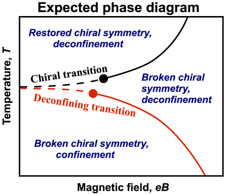
In our effective model, PLSMq, we compute and discuss each one-loop contribution to the effective potential for the approximate order parameters of the chiral and deconfining transitions, given by the chiral condensate and the expectation value of the Polyakov loop, respectively. We treat the external magnetic field, that plays the role of a thermodynamic control parameter, as a constant and uniform field, and make no assumption on its intensity. In Fig. 1 we show a cartoon of the temperature–magnetic field phase diagram one would expect from previous results for the limits of strong and weak fields, for chiral and deconfining transitions treated separately, as discussed below.
Modifications in the vacuum of strong interactions by the presence of an external magnetic field have been investigated previously within different frameworks, mainly using effective models Klevansky:1989vi ; Gusynin:1994xp ; Babansky:1997zh ; Klimenko:1998su ; Semenoff:1999xv ; Goyal:1999ye ; Hiller:2008eh ; Ayala:2006sv ; Boomsma:2009yk , especially the NJL model Klevansky:1992qe , and chiral perturbation theory Shushpanov:1997sf ; Agasian:1999sx ; Cohen:2007bt , but also resorting to the quark model Kabat:2002er and certain limits of QCD Miransky:2002rp . Most treatments have been concerned with vacuum modifications by the magnetic field, though medium effects were considered in a few cases, as e.g. in the study of the stability of quark droplets under the influence of a magnetic field at finite density and zero temperature, with nontrivial effects on the order of the chiral transition Ebert:2003yk . Magnetic effects on the dynamical quark mass Klimenko:2008mg , as well as magnetized chiral condensates in a holographic description of chiral symmetry breaking holographic , were also considered. Lattice simulations were also used to demonstrate an enhancement of the chiral condensate and the appearance of chiral magnetization of the chirally broken vacuum under the influence of a strong magnetic field lattice . Ring-diagram corrections to the effective potential in a weak magnetic field were considered in Ref. ring . Recent applications of quark matter under strong magnetic fields to the physics of magnetars using the NJL model can be found in Ref. Menezes:2008qt ; Menezes:2009uc .
The case of the thermal quark-hadron transition in a magnetic field was studied recently in Ref. Agasian:2008tb . It was found that the critical temperature and the latent heat are both diminished in the presence of the magnetic field, and that the first-order deconfining turns into a crossover at sufficiently strong magnetic fields. On the other hand, it has been shown in Ref. Fraga:2008qn that the chiral transition can be dramatically modified in the presence of a strong magnetic field. In particular, the smooth crossover found for vanishing baryonic densities can be turned into a first-order phase transition if the magnetic field is sufficiently high, the threshold being close to fields that can be achieved in current and future heavy ion collision experiments. For the chiral transition – on the contrary to the case of the deconfining transition of Ref. Agasian:2008tb – the critical temperature seems to increase with the magnetic field, thus favoring a first-order behavior, which goes in line with the theoretical expectation on the role played by magnetic fields in the nature of phase transitions landau-book . On the other hand, at very weak magnetic field both confinement and the chiral transitions should again be crossovers Aoki:2006we . This justifies our preliminary approximate cartoon of Fig. 1.
More recently, the chiral magnetic effect was also studied in the context of the PNJL model Fukushima:2010fe . Here we propose a different effective theory for the study of the phase structure of QCD in the presence of an external magnetic field, the linear sigma model coupled to quarks and to the Polyakov loop, and compute the phase diagram in the presence and, separately, in the absence of vacuum corrections. The contribution from these corrections is very large, though the issue of their relevance or necessity is non-trivial in this context as also in different ones, such as the Higgs potential in the electroweak theory and the Walecka model in high-density nuclear physics FTFT-books . We choose to present results in both scenarios and address the issue in the end. Nevertheless, we believe that lattice results will be crucial in setting the most appropriate effective theory approach. The PLSMq can, of course, also be used to study chiral symmetry breaking and deconfinement in the absence of a magnetic field. We present a few results in this case but, keeping our focus on the phase structure in the presence of a magnetic background, leave a thorough study for a future publication next .
The paper is organized as follows. In Section II we provide a description of the effective theory that allows us to study the influence of an external magnetic field on confining and chiral properties of QCD, the linear sigma model coupled to quarks and to the Polyakov loop (PLSMq). We discuss the quark, chiral and confining sectors, the total free energy and the connection to various observables. In Section III we compute all one-loop contributions to the effective potential, discussing vacuum and thermal corrections in detail. Section IV contains our results for the effective potential and a discussion of the temperature–magnetic field phase diagram. Section V contains our conclusions and outlook.
II Effective theory
II.1 Quark, chiral and confining variables
The effective field theory that we denote by PLSMq has three types of variables: the quark field , the chiral field and the Polyakov loop variable .
The confining properties of QCD are described by the complex-valued Polyakov loop variable , which plays the role of an approximate order parameter for the confining phase transition in QCD. The Polyakov loop is a singlet part of the matrix (“untraced Polyakov loop”) which belongs to the adjoint representation of the color group, i.e.:
| (1) |
where is the matrix-valued temporal component of the Euclidean gauge field and the symbol denotes path ordering. The integration takes place over compactified imaginary time .
The expectation value of the Polyakov loop is an exact order parameter of the color confinement in the limit of infinitely massive quarks:
| (4) |
The chiral features of the model are encoded in the dynamics of the chiral field
| (5) |
where is the isotriplet of the pseudoscalar pion fields and is the chiral scalar field which plays the role of an approximate order parameter of the chiral transition. The expectation value of the field is an exact order parameter in the chiral limit, in which quarks and pions are massless degrees of freedom:
| (8) |
The up and down fields of the constituent quarks are grouped together into the doublet fermion field
| (11) |
which plays a central role in our discussion. The fermion field couples two other variables, the Polyakov loop and the chiral field to each other, thus linking confining and chiral properties together. The quarks are also coupled to the external magnetic field since the and quarks are electrically charged. Since the quarks are also coupled to the Polyakov loop and the chiral field , it is clear that the external magnetic field will affect the chiral dynamics and the confining properties of the model. Thus, this model allows us to investigate the influence of the external magnetic field on color confinement and chiral symmetry breaking simultaneously.
We can write the Lagrangian of PLSMq as follows:
| (12) |
II.2 Quark sector
The first part of the full Lagrangian (12),
| (13) |
describes the constituent quarks, which interact with the meson fields , the Abelian gauge field and the gauge field via the covariant derivative:
| (14) |
The Abelian gauge field describes the influence of the external magnetic field aligned along the third direction, , for convenience:
| (15) |
and the electric charges of the quarks are defined by the following matrix:
| (20) |
where is the elementary electron charge.
The gauge field represents a nontrivial background due to the Polyakov loop (1). It is convenient to diagonalize the untraced Polyakov loop . In this gauge the field , which enters the quark Lagrangian (13), is diagonal:
| (21) |
where are the Cartan generators of the gauge group. The gauge field is prescribed to take constant values, being linked to the Polyakov loop as follows:
| (22) | |||||
with
| (26) |
II.3 Chiral Lagrangian
The chiral part of the PLSMq Lagrangian is given by the second term of Eq. (12), that can be written in the Minkowski space-time as follows:
| (27) |
Here we have introduced the charged and neutral mesons, respectively,
| (28) |
The electric charges of the -mesons are , so that the covariant derivative in Eq. (27) reads
| (29) |
This derivative does not involve the Polyakov loop, contrary to the covariant derivative acting on quarks (14), since the pions are colorless states.
In Eq. (27), stands for the potential of the chiral fields. This potential exhibits both spontaneous and explicit breaking of chiral symmetry:
In the second line of this equation we explicitly show the quadratic form of the potential which provides the masses to the meson fields. Here, the masses and correspond to the vacuum masses of the sigma and the pion mesons, which are used to fix the parameters and in the classical potential, since is also known, as explained below.
As customary in the linear sigma model, we follow a mean-field analysis in which the mesonic sector is treated classically whereas quarks represent fast degrees of freedom. The parameters of the Lagrangian (27) are chosen to match the low-energy phenomenology of mesons in the absence of magnetic fields and at zero temperature, i.e. in the vacuum sigma-model . Using the notation of Ref. Scavenius:2000qd , this implies the following expectation values for the condensates: and , with and . The masses in Eq. (II.3) should be considered as parameters of the model, which coincide with corresponding meson masses at and .
The explicit symmetry breaking term, as usual, is determined by the PCAC relation , so that and in the vacuum. Choosing the value of the quartic interaction , one gets a reasonable -mass . The constituent quark mass is given by , and, choosing at , one obtains for the constituent quarks in the vacuum . At low temperatures the quarks are not excited, and the model (27) reproduces results from the usual linear -model without quarks FTFT-books .
If the explicit symmetry breaking term is absent, , then the model (27) experiences a second-order phase transition Pisarski:1983ms from the broken symmetry phase to the restored phase at a critical temperature . The presence of the explicit symmetry breaking term changes the phase transition into a smooth crossover.
The pion directions play no major role in the process of phase conversion we have in mind, as was argued in Ref. Scavenius:2001bb for the case of the chiral transition. Therefore in what follows we focus on the sigma direction of the chiral sector. However, the coupling of charged pions to the magnetic fields might be quantitatively important in a possible development of charged chiral condensates. This issue, though, makes the computation technically much more involved and will be addressed in a future publication next .
II.4 Confining potential
We choose to couple the Polyakov loop to the linear sigma model in the same fashion as was successfully implemented in the case of the Nambu–Jona-Lasinio model in Refs. ref:fukushima ; ref:ratti07 ; ref:ratti08 . The confining properties of the system in our model are accounted for by the third term in Eq. (12), which describes the Polyakov loop variable (1):
| (31) |
We treat the Polyakov loop in a mean-field approach, neglecting a kinetic term for this variable. Although the Polyakov loop is, strictly speaking, a static quantity, a kinetic term is often added to describe the dynamics in an effective model for deconfinement Meisinger:2002kg ; Fraga:2006cr .
Notice that, in our approach, the Polyakov loop variable is not coupled to the chiral variables in the bare Lagrangian (31). The reason is that the chiral variables are colorless degrees of freedom which should not affect the Polyakov loop at least in a first approximation. Of course, the mesons are made of colored quarks which do feel colored degrees of freedom like . Thus, the interaction between the chiral and confining variables will inevitably appear later, after the quarks are integrated out. This approach is not unique. In fact, it is common to couple the Polyakov loop directly to chiral fields phenomenologically as a way to link the chiral and deconfining transitions in a generalized Landau-Ginzburg theory, in which the behavior of an order parameter induces a change in the behavior of non-order parameters at the transition via the presence of a possible coupling between the fields Dumitru:2000in ; Mocsy:2003tr ; Megias:2004hj .
The term (31) is essentially the potential term of the Polyakov action in the pure Yang-Mills theory not coupled to quarks. Quark effects manifest via coupling with the quark matter field in the first part of our Lagrangian, Eq. (13).
The effective potential (31) has the following properties: it should satisfy the center symmetry,
| (32) |
which is realized in the limit of the pure gauge theory (the coupling to dynamical quarks break this symmetry). According to Eq. (4), the potential (31) should have an absolute minimum at in the confined phase. Results from lattice simulations ref:Lattice:Tc show that the deconfining transition in gauge theory takes place at a critical temperature . As the system undergoes the phase transition the single minimum at of the potential splits into three degenerate minima labeled by the variable. As a consequence, in the deconfined phase the symmetry is spontaneously broken, and .
Following Ref. ref:ratti08 we use a specific form for the phenomenological potential of the Polyakov loop:
| (33) | |||
with
| (34) | |||||
| (35) |
where is the critical temperature in the pure gauge case: .
The phenomenological parameters in Eq. (35) are
| (38) |
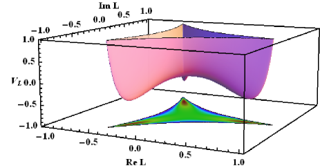
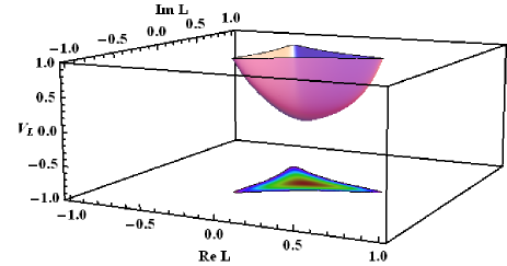
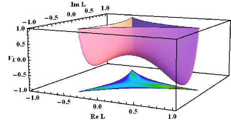
Consistently with the original definition (1), the potential (33) limits the values of the Polyakov loop to the interval because of a logarithmic divergence in (33). The value is reached in the limit . In the confined phase, , the potential has one trivial minimum [as illustrated in Figure 2 (top)], whereas in the deconfined phase, , the potential has three degenerate minima [see Fig. 2 (bottom)]. The latter are mutually connected by transformations.

The set of parameters (38) is obtained by demanding the following requirements valid for pure gauge theory ref:ratti08 :
-
(i)
the Stefan-Boltzmann limit is reached at ;
-
(ii)
a first-order phase transition takes place at ;
-
(iii)
the potential describes well lattice data for the Polyakov loop and for the thermodynamic functions such as pressure, energy density and entropy.
The uncertainties for the parameters in Eq. (38) are: for , less than for , and about for ref:ratti08 .
II.5 Total free energy and observables
The free energy of the system is given by
| (39) |
where is the spatial volume and is the partition function
| (40) |
In the mean field approximation, treating the meson fields classically and keeping only the sigma direction in the mesonic sector, the free energy is given by
where the potential for the chiral field is given in Eq. (II.3) and the potential for the Polyakov loop is defined by Eq. (33). In (LABEL:eq:Omega) we explicitly show the dependence of the free energy on the external magnetic field , the temperature , and the mean field value of the chiral field , as well as the expectation value of the Polyakov loop .
The temperature and the magnetic field impose the fixed external conditions whereas the expectation values of the dynamical fields are obtained by minimization of the free energy (LABEL:eq:Omega) with respect to the dynamical variables:
| (42) |
The mass of the -mesons is given by the curvature of evaluated at the global minimum (42) of the free energy, i.e.:
| (43) |
Notice that the mass (43) depends implicitly on the temperature and the strength of the magnetic field . The zero-temperature and zero-field value of the -meson mass (defined in the preceding Section) is related to Eq. (43) as follows .
III Free energy at one loop
We compute the free energy of the system in the one-loop approximation. To this end, we functionally integrate over the quark fields and take the integral over the fluctuations of the mesonic degrees of freedom near the minimum of the free energy, determined by Eq. (42). These integrals yield thermal determinants, either in the background of the magnetic field or for vanishing field.
The one-loop correction coming from quarks can be written in the form:
| (44) | |||||
where the quark Lagrangian is given in Eq. (13). The notation “” means that the determinant is taken at nonzero temperature, while “” indicates that we consider the case.
The numerator in Eq. (44) involves the covariant derivative (14) because we calculate the contribution of the fermion loop in the presence of an external magnetic field and in the background of the nontrivial Polyakov loop. The magnetic field and the Polyakov loop affect the chiral degrees of freedom via the covariant derivative. Thus, the integration over quark fields provides an effective potential for the meson fields, and , and the Polyakov loop, . The coefficients of this potential should in general depend on the strength of the magnetic field and on the temperature . The determinant in the numerator of Eq. (44) is regularized by a similar determinant in the denominator which is calculated at , and in the absence of the confining background. Thus, the quark one-loop correction is expressed in terms of a ratio of fermionic determinants. In what follows we assume that the vacuum of the model is defined by , .
Following Ref. Agasian:2008tb it is convenient to regroup in Eq. (44) the ratio of the determinants, and represent the free energy of each species of the light quarks as follows:
| (45) | |||||
where stands for either or . The first ratio corresponds to the response of the quark loops to the external fields at zero temperature. This term represents the vacuum contribution, . The second ratio in Eq. (45) represents the finite-temperature correction due to thermal fermion excitations. As in Ref. Agasian:2008tb , we call this contribution the paramagnetic part of free energy, .
In this paper, as mentioned previously, we consider two approaches for the PLSMq, one that includes -dependent vacuum effects and one that does not. We intentionally ignore pure vacuum corrections, in order to compare our results with what is found in the absence of a magnetic background in the literature of the linear sigma model with quarks, coupled or not to Polyakov loops (e.g., Ref. Scavenius:2000qd ). However, since this is a theory with spontaneous symmetry breaking (besides an explicit breaking), a nonzero condensate modifies the quark mass, and vacuum subtractions are more subtle. At the end, there are finite logarithmic contributions that survive renormalization, sometimes called zero-point corrections, but that are usually discarded phenomenologically in the LSMq. These contributions have been studied by the authors of Ref. Mocsy:2004ab in the LSMq. Vacuum contributions were considered at finite density in the perturbative massive Yukawa model with exact analytic results up to two loops in Ref. Palhares:2008yq ; thesis and, more specifically, in optimized perturbation theory at finite temperature and chemical potential in Ref. Fraga:2009pi , also comparing to mean-field theory. More recently, this issue was discussed in a comparison with the Nambu-Jona–Lasinio model Boomsma:2009eh . A very recent careful and detailed study in the (Polyakov loop extended) quark-meson model, with special attention to the chiral limit, can be found in Refs. Skokov:2010wb .
Thus, the one-loop correction from quarks to the free energy of the system is given by
| (46) |
Below we discuss each term in this equation separately.
III.1 Vacuum contribution,
The vacuum contribution can be expressed as the Heisenberg–Euler energy density111In Ref. ref:review:Dunne one can find results for spinor and scalar determinants in the presence of external fields.:
where we have already accounted for the color degeneracy of the quark degrees of freedom.
Since the covariant derivative contains not only the electromagnetic but also the non-Abelian gluon fields, one could expect that non-Abelian features should also appear in Eq. (III.1). Notice, however, that the Polyakov loop contribution is trivial since, for , it can be put away by a simple shift in the integral over the zeroth component of the momentum. So, for the vacuum contribution from quarks we can ignore its presence in the covariant derivative. On the other hand, as we discuss below, at non-zero temperature the presence of the gluon field leads effectively to a shift of the Matsubara frequencies, thus contributing to the paramagnetic (second) part of (46).
The expression above corresponds, of course, to the quark vacuum correction in the presence of the external magnetic field
| (48) | |||||
minus the vacuum correction in the absence of the field
| (49) |
where we have defined the integral
| (50) |
and the quark mass in the presence of
| (51) |
One can control the divergences in the integrals above via dimensional regularization and compute the difference in the scheme, obtaining
| (52) | |||||
where , is the derivative with respect to the first argument of the Riemann-Hurwitz function AS , and is the renormalization subtraction scale. This expression is in agreement with the results of Refs. Ebert:1999ht ; Menezes:2008qt , except for the scale-dependent term. Since the scale-dependent term is independent of the meson fields and we are concerned only with the effective potential of the theory, we can discard it. Here our normalization is such that this correction vanishes in the limit of . One arrives at the same result using the Heisenberg-Euler approach and imposing the normalization mentioned above.
We can cast the correction to the effective potential in a dimensionless form normalizing every quantity by a mass scale. For this purpose, we choose as our mass unit and define:
| (53) |
It is also convenient to write the quark electric charge as , so that and . Then, the vacuum one-loop contribution to the effective potential is given by
| (54) |
where the function is defined as
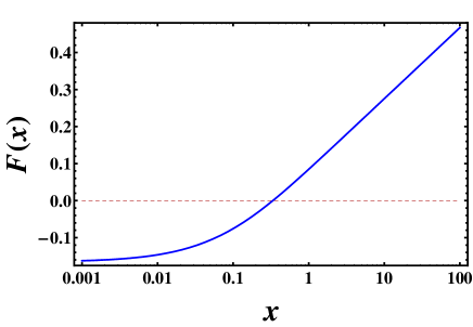
| (55) |
and displayed in Figure 3. For small values of its argument it behaves as
| (56) |
whereas for large a argument one finds
| (57) |
Since the constituent quark mass is linear in , the external magnetic field modifies the classical potential (II.3) for the field. One can see from the behavior of this correction that its effect is to increase the value of the condensate and deepen the absolute minimum of the effective potential, as expected from previous results on magnetic catalysis.
Finally, for the sake of completeness, we discuss the weak and strong field limits of the quark free energy (III.1). The leading term in the weak-field limit () is
| (58) |
The strong-field limit () with on-shell renormalization () is given by ref:review:Dunne :
where , , , is the Euler constant, and is the Glaisher constant222In Ref. Fraga:2008qn , the quark vacuum term was not included, the charged pions vacuum contribution being considered instead. Both treatments increase the value of the condensate and deepen the effective potential. In this paper we choose to treat the mesonic fields classically..
Numerical tests show that only in the limit of very high fields, in units of , the vacuum corrections bring a non-negligible modification to the effective potential.
III.2 Paramagnetic contribution,
The paramagnetic temperature-induced contribution comes from the second determinant ratio in Eq. (45). In general, a quark determinant can be formally written as the product over the eigenvalues of the corresponding Dirac operator, i.e.:
| (60) |
where satisfy the eigenvalue equation
| (61) |
It is important to stress that in Eq. (60) we omitted a -independent constant which would anyway be subtracted at the end of the calculation.
The algebraic equation for eigenvalues reads as follows:
| (62) |
where is the electric charge of the quark, is the quantum number that labels the Landau levels and is the projection of the spin of the quark eigenstate onto the -axis. Here is the th diagonal component of the gauge field. We assume no sum over color indices unless explicitly indicated. From (62) one finds
| (63) |
At zero magnetic field the contribution to the effective potential coming from (60) can be written as follows:
| (64) |
where labels the Matsubara frequencies . The zeroth component of the momentum is related to the Matsubara frequency as follows:
| (65) |
where the odd frequency takes into account the anti-periodicity of the quark fields along the temporal direction.
In the presence of a magnetic field , the integral over the phase space in Eq. (64) is modified to
| (66) |
where the integer labels the Landau levels.
Using the mapping (66), the explicit expression for the fermion determinant (64) and the eigenvalues (63), we can rewrite the quark-induced potential (45) as follows:
where the dispersion relation for quarks in the external magnetic field is
| (68) |
with constituent quark mass .
With a suitable identification, and , the sum over Matsubara frequencies in Eq. (III.2) can be done explicitly with the help of the following formula (with arbitrary real and ):
| (69) | |||
The first term in the right hand side of equation above is divergent. In the language of the effective potential (III.2), the divergent term corresponds to a contribution from massless fermions plus an additive constant. We ignore this term since it depends neither on chiral nor on confining variables. The second term leads to a –independent contribution to (III.2), which is already taken into account by the vacuum energy (III.1). The last two terms lead to the regularized paramagnetic free energy for the chiral and confining fields:
| (70) |
where
Here the trace Trc is taken in the color space and the angles are defined in the diagonal representation (22) of the untraced Polyakov loop [the Polyakov loop is defined in Eq. (1)]. Notice that the parameters – which are the phases of the diagonal components of the untraced Polyakov loop – enter the partition function exactly like imaginary chemical potentials.
The paramagnetic contribution, given by Eqs. (70) and (III.2), can be simplified further by expanding the logarithmic function in Eq. (III.2) in the following series:
| (72) |
Next, we use the simple relation
| (73) |
where is the modified Bessel function of the second kind (the MacDonald function) and order AS . Finally, we express the free energy (70) in terms of the sums only:
| (74) | |||||
where is the energy of the th Landau level (68) at zero longitudinal momentum
| (75) |
and the untraced Polyakov loop is defined in Eq. (22), so that
| (76) |
The integer number corresponds to the winding number of the Polyakov loops.
It is also convenient to express the paramagnetic contribution to the effective potential in terms of dimensionless quantities as follows:
| (77) |
where we defined the dimensionless function
| (78) | |||||
and the dimensionless version of Eq. (75), i.e.
| (79) |
III.3 Paramagnetically-induced breaking of
One can see from Eq. (74) that the magnetic field drastically affects the potential for the Polyakov loop. Take, for example, the limit of a very strong field, . Then, the leading contribution to Eq. (74) is given by the lowest Landau level, , with spins oriented along the field, , at lowest winding number of the Polyakov loop, . Thus, the leading term of the strong-field expansion of the paramagnetic potential (74) is
| (80) |
where the Polyakov loop variable is defined in Eq. (1). At fixed value of the magnetic field and temperature, the function (80) is a nonmonotonic function of the field : it increases at small values of and decreases at large values of . This fact will be essential for our discussion of the role of the vacuum contribution introduced in the previous subsection: the vacuum contribution makes the expectation value of the field larger, eventually diminishing the role of the paramagnetic contribution (80) at large enough magnetic fields.
Notice that the paramagnetic contribution (80) is not invariant under the symmetry, and therefore the paramagnetic contribution (80) deforms the potential for the Polyakov loops. So, it is clear that the magnetic field tends to break the symmetry and induce deconfinement in this model.
In order to illustrate the effect of the paramagnetic term (74) we plot in Figure 4 the potential for the Polyakov loop (33) including the correction induced by the paramagnetic interaction (80). In the figure, The magnetic field is . We show the potential for two temperatures, and , in order to compare the plots with the pure gauge field potential displayed in Figure 2. The effect of the magnetic field is clearly seen in the deconfined phase: the paramagnetic interaction induces the expectation value of the Polyakov loop to be real-valued.
III.4 Complete effective potential
It is, of course, also convenient to define dimensionless expressions for the classical potential
| (81) |
where , and for and the potential for the Polyakov loops
| (82) |
where we used Eq. (33) and defined , besides expressing and in terms of and .
The total (dimensionless) effective potential can then be expressed as
and it is this form of the effective potential that we use to determine the phase structure of the PLSMq effective field theory in the following section.
IV Phase structure
In our numerical analysis we have considered the following situations:
-
(A)
The linear sigma model with thermal corrections, without the coupling to the Polyakov loop. This is a standard analysis and has been performed previously in quarks-chiral ; ove ; Scavenius:1999zc ; Caldas:2000ic ; Scavenius:2000qd ; Scavenius:2001bb ; paech ; Mocsy:2004ab ; Aguiar:2003pp ; Schaefer:2006ds ; Taketani:2006zg ; Fraga:2004hp , and it is shown here for the sake of completeness;
-
(B)
The linear sigma model at finite temperature coupled to the Polyakov loop. At this point the effects of the magnetic field were not taken into account yet and we investigated only the effects of the interaction between the two order parameters;
-
(C)
The linear sigma model in a magnetic background at zero temperature. In this case the Polyakov loop is excluded by construction. The magnetic field manifests itself through vacuum corrections from the quarks;
-
(D)
The complete scenario: the linear sigma model coupled to the Polyakov loop with thermal corrections in the presence of a magnetic background.
In the latter case we also investigated the effects of including vacuum corrections or not. The discussion about the inclusion or not of such terms is still inconclusive, not being clear which treatment is closer to the original theory, QCD. We obtained phase diagrams in the plane for both cases and verified that the inclusion or not of vacuum corrections is crucial to the structure of the phases, influencing not only the nature of the transitions, as it was first observed in Boomsma:2009eh , but also changing the qualitative behavior of the transition lines.
IV.1 ,
This case is described by the linear sigma model coupled to quarks. We take into account thermal corrections and disregard coupling to the Polyakov loop (22). The chiral condensate is the approximate order parameter for the chiral transition, and for low temperatures it is nonzero, indicating symmetry breaking. The value in the vacuum is adjusted to correspond to the pion decay constant, , as described in section II.3. As the temperature is raised the minimum approaches zero, and for high enough the symmetry is recovered. As the position of the minimum as a function of temperature is continuous, and so is its derivative, the transition is a crossover.
IV.2 , ,
In this subsection we analyze the interaction between the chiral condensate and the Polyakov loop, without the presence of the magnetic field. The treat the model at finite temperature because of the presence of the Polyakov loop (22) in the formulation of the model. The expression for the thermal effective potential is similar to Eq.(70):
| (84) |
where has an expression similar to Eq.(III.2), but the frequency has no dependence on the magnetic field, and is given by .
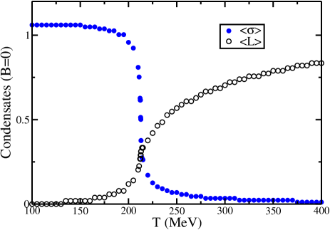
Due to the interaction, the degeneracy is broken and the minimum along the real axis becomes the global one. Both transitions, chiral and deconfinement, are consistent with a crossover-type transition since the order parameters behave as smooth functions of the temperature, Fig. 6. The slopes of both order parameters becomes steepest at the same temperature , clearly showing the tight relation between the order parameters.
IV.3 ,
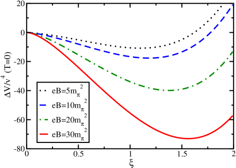
At zero temperature the Polyakov loop is absent by construction. The only pieces of effective potential that contribute are the linear sigma model potential and the vacuum correction from quarks. The magnetic field influencing the system through the latter. We plot in Fig. 7 the effective potential for different values of the external magnetic field. We can see that as the field increases in magnitude the potential becomes deeper and the value of the condensate raises, in accordance with results at zero temperature that indicate an enhancement of chiral symmetry breaking. This effect – known as magnetic catalysis – is in accordance with previous result from two of us Fraga:2008qn . In Fig. 7 we subtracted the value of the potential with , in order to have a better comparison for different values of magnetic field, and is the resultant potential. This procedure will be applied in all plots of the effective potential along this section.
IV.4 , ,
Finally we analyze the full potential. It contains the linear sigma model, the pure gauge potential, thermal corrections including interaction between the two fields, and vacuum corrections from the quarks. The effects of including or not the vacuum terms were also considered and have shown to be crucial for the structure of phases. The relevant potential is given in Eq. (LABEL:eq:Veff-dim). This potential is a function of the parameters , , and , where we used the parameterization (22) and set . As shown in Fig. 2, for pure gauge the potential – written in terms of and – has three degenerated minima. It is known that in the presence of quarks this degeneracy is broken and the global minimum will be in the direction of . Since we are interested only in the minima of the potential, we can simplify our analysis by setting to be zero.
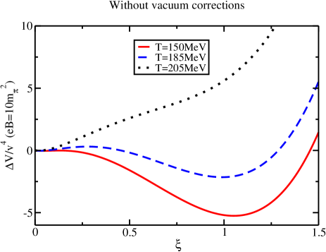
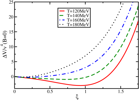
Let us consider first the potential without vacuum corrections. We evaluate it for different values of magnetic field and temperature. For each set of values of and we minimize the potential with respect to and . Then we use this value of to plot the effective potential as a function of only. Figure 8 illustrated the evolution of the chiral transition at the magnetic field . Initially the condensate has a non-zero expectation value and this value decreases as the temperature increases. Then, a local minimum appears for , and above a certain critical temperature it becomes the global minimum. The barrier between the two minima causes a discontinuity in the expectation value of , pointing out to a first order character of the chiral transition, in accordance with Fraga:2008qn . In the same way as in the case , , the potential becomes deeper for high values of the magnetic field. However, the thermal corrections, responsible for restoring chiral symmetry, also acquire a higher magnitude, bringing the chiral critical temperature down.
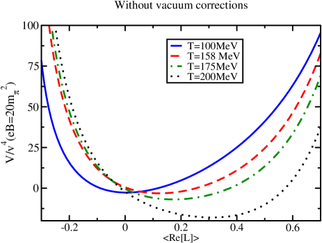
In Fig. 9 we fix at its minimum for a set of values of and , and plot the potential as a function of . We can then follow the evaluation of the expectation value of the parameter . At low temperatures it is zero, indicating confinement, and above a critical temperature it goes asymptotically to one. At the critical value of the temperature, where the chiral transition occurs, the variable also presents a discontinuity, so that the first-order chiral transition is accompanied by a first-order deconfinement transition for large strengths of the magnetic field. Thus, if the vacuum corrections are not taken into account, then the magnetic field enhances the order of the phase transition and the transition changes from the crossover type (realized at , Section IV.2) to the first order type.
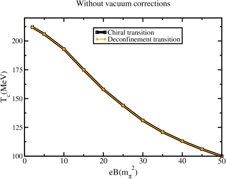
The phase diagram for the potential described above is shown in Fig. 10 333 The starting point of the curve – given by the critical temperature at zero chemical potential – is somewhat higher compared to the value obtained in recent numerical calculations of lattice QCD with two flavors of light fermions (see, for instance, the review ref:Karsch ). Generally, effective models like our PLSMq or the PNJL model give approximate answers for particular quantities while being able to predict a general picture at a very good qualitative level.. The critical temperature for the chiral and deconfinement transitions are the same for different values of magnetic field, resulting in two phases: a confined phase with broken chiral symmetry, and a deconfined phase with restored chiral symmetry. The common critical line of these phase transitions is of first order for all values of the magnetic field except for very small values of . As the magnetic field decreases, the transition turns back into a crossover reproducing the physical situation with that was discussed around Fig. 6.
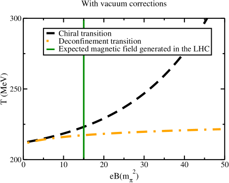
The inclusion of vacuum corrections from quarks changes the phase diagram dramatically. Following the same procedure describe above, we plot the potential as a function of in Fig. 11 and as a function of in Fig. 12. The corresponding phase diagram is shown in Fig. 13. The vertical green line indicates the value of magnetic field that is expected to be reached in heavy-ion collisions in the ALICE experiment at the LHC Skokov:2009qp .
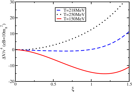
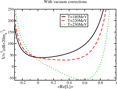
The presence of the quark vacuum term changes the order of the chiral transition, turning it into a crossover. In the case without the vacuum correction, the transition was of first order due to thermal effects. The thermal contribution generates a minimum at being rather sensitive to the value of the magnetic field. In the present case, however, the vacuum term has a magnitude that is larger compared to the thermal piece. Thus, the vacuum contribution dominates the position of the minimum, and it is the vacuum part that is responsible for driving the transition to a crossover. Moreover, the chiral-violating property of the vacuum quark contribution overwhelms the chiral-restoration tendency of the thermal part so that the critical temperature of the chiral transition – calculated by taking into account both vacuum and thermal effects – becomes an increasing function of the external magnetic field.
It is interesting to recall that the thermal contribution of quarks tends to destroy the confinement at strong magnetic fields, Fig. 10, contrary to the confinement-enhancing property of the vacuum contribution. This effect is due to the fact that the vacuum contribution makes the value of the field larger (as one can see in Fig. 7), suppressing the violating paramagnetic contribution (80) at large enough magnetic fields. Thus, large magnetic fields tend to enhance the confinement property of the vacuum. As in the case of the chiral transition, the vacuum contribution exceeds its thermal counterpart so that the deconfinement transition temperature appears to be a weakly increasing function of the magnetic field, Fig. 13. The confinement transition is also a crossover.
The lines of the confinement and chiral transitions coincide for small values of , and go apart as the field increases in magnitude. Results from lattice QCD indicate that in the absence of the magnetic field the deconfinement transition and chiral symmetry restoration happen in the same narrow temperature interval ref:Karsch:coincide . Our calculations indicate that the presence of a strong magnetic field should inevitably split these transitions in this case.
The deconfinement transition occurs at lower temperatures compared to the temperature of chiral restoration. Thus, in a strong magnetic field a deconfined phase with broken chiral symmetry should appear. The splitting between these transitions becomes wider with the increase of the magnetic field . Some other approaches Agasian:2008tb – that were not taking into account vacuum corrections – demonstrate that (i) the deconfinement temperature drops down as the magnetic field increases; and that (ii) at some critical value of the magnetic field, , color confinement may disappear as illustrated in Fig. 1. On the contrary, we show that the inclusion of the mentioned vacuum corrections make the critical deconfining temperature to be an increasing function of the magnitude of the magnetic field up to . We have not found a signature of a critical magnetic field that would lead to the magnetic-field-induced deconfining transition in either scenario, with and without vacuum corrections.
V Conclusion
In this paper we studied the influence of a strong magnetic field background on confining and chiral properties of QCD, using the linear sigma model coupled simultaneously to quarks and to the Polyakov loop (PLSMq). This model associates electromagnetic, chiral and the confining degrees of freedom in a natural way.
In the confining sector, the strong magnetic field affects the expectation value of the Polyakov loop, which is an approximate order parameter for the confinement–deconfinement phase transition at finite temperature. We found that the contribution from the quarks to the Polyakov-loop potential has three features:
-
1.
the presence of the magnetic field breaks the global symmetry and makes the Polyakov loop real-valued (this effect is seen in the Polyakov loop potential, Fig. 4);
-
2.
the thermal contribution from quarks tends to destroy the confinement phase by increasing the expectation value of the Polyakov loop;
-
3.
on the contrary, the vacuum quark contribution tends to restore the confining phase by lowering the expectation value of the Polyakov loop.
The vacuum correction from quarks has a crucial impact on the phase structure. If one ignores the vacuum contribution from the quarks, then one finds that the confinement and chiral phase transition lines coincide, Fig. 10, and in this case the increasing magnetic field lowers the common chiral-confinement transition temperature. However, if one includes the vacuum contribution, then the confinement and chiral transition lines split, and both chiral and deconfining critical temperatures become increasing functions of the magnetic field, Fig. 13. The vacuum contribution from the quarks affect drastically the chiral sector as well.
Our calculations also show that the vacuum contribution seems to soften the order of the phase transition: the first-order phase transition – which would be realized in the absence of the vacuum contribution – becomes a smooth crossover in the system with vacuum quark loops included.
It is important to stress that in a strong magnetic field a deconfined phase with broken chiral symmetry will appear in the scenario with quark vacuum corrections. The splitting of the confinement and chiral transitions – as shown in Fig. 13 – may be substantial at a steady magnetic field of the magnitude that is expected to be realized in heavy-ion collisions. For example, in the ALICE experiment at the LHC facility, the magnetic field may peak around the value Skokov:2009qp . We find (see Fig. 13) that the splitting between the critical temperatures of the confinement and chiral crossovers in a constant field of the typical LHC magnitude may reach the noticeable value
Deciding whether quark vacuum contributions should be included or not is, unfortunately, an open issue yet. Lattice simulations of QCD with dynamical fermions in the presence of a magnetic field could certainly shed some light onto this matter. Recent lattice results seem to favor the scenario that takes into account the vacuum contributions delia .
Note added. After this paper was submitted to the journal, a new preprint on a similar subject has appeared Gatto:2010qs . The authors have found a splitting of the deconfinement and chiral transitions in the magnetic field background in the framework of a Polyakov-loop extended Nambu-Jona Lasinio model with eight-quark interactions. This independent result is an agreement with our conclusion on splitting of these transitions in the linear -model (with the vacuum corrections included).
Acknowledgements.
A.J.M. is especially grateful to J. Boomsma for intense and valuable discussions. The authors are also indebted to D. Boer, M. D’Elia, K. Fukushima and D. Kharzeev. A.J.M. and E.S.F. thank the LMPT at Université de Tours, and E.S.F is grateful to the members of the theory group at Vrije Universiteit Amsterdam, where part of this work has been done, for their kind hospitality. The work was partially supported by CAPES/COFECUB project number 663/10. The work of E.S.F. and A.J.M. is partially supported by CAPES, CNPq, FAPERJ, and FUJB/UFRJ. The work of M.N.C. is partially supported by the French Agence Nationale de la Recherche project ANR-09-JCJC “HYPERMAG”.References
- (1) Proceedings of the 5th International Workshop on Critical Point and Onset of Deconfinement (CPOD 2009), PoS(CPOD 2009).
- (2) R. C. Duncan and C. Thompson, Astrophys. J. 392, L9 (1992); C. Thompson and R. C. Duncan, ibid. 408, 194 (1993).
- (3) D. J. Schwarz, Annalen Phys. 12, 220 (2003). [arXiv:astro-ph/0303574].
- (4) D. Kharzeev, R. D. Pisarski and M. H. G. Tytgat, Phys. Rev. Lett. 81, 512 (1998) [arXiv:hep-ph/9804221]. D. Kharzeev and R. D. Pisarski, Phys. Rev. D 61, 111901(R) (2000) [arXiv:hep-ph/9906401]; K. Buckley, T. Fugleberg and A. Zhitnitsky, Phys. Rev. Lett. 84, 4814 (2000) [arXiv:hep-ph/9910229]; S. A. Voloshin, Phys. Rev. C 62, 044901 (2000) [arXiv:nucl-th/0004042]; S. A. Voloshin, Phys. Rev. C 70, 057901 (2004) [arXiv:hep-ph/0406311]; D. Kharzeev, Phys. Lett. B 633, 260 (2006) [arXiv:hep-ph/0406125]; D. Kharzeev and A. Zhitnitsky, Nucl. Phys. A 797, 67 (2007) [arXiv:0706.1026 [hep-ph]].
- (5) D. E. Kharzeev, L. D. McLerran and H. J. Warringa, Nucl. Phys. A 803, 227 (2008) [arXiv:0711.0950 [hep-ph]]; K. Fukushima, D. E. Kharzeev and H. J. Warringa, Phys. Rev. D 78, 074033 (2008) [arXiv:0808.3382 [hep-ph]]; D. E. Kharzeev and H. J. Warringa, Phys. Rev. D 80, 034028 (2009) [arXiv:0907.5007 [hep-ph]]; D. E. Kharzeev, Nucl. Phys. A 830, 543C (2009) [arXiv:0908.0314 [hep-ph]]; D. E. Kharzeev, Annals Phys. 325, 205 (2010) [arXiv:0911.3715 [hep-ph]]; K. Fukushima, D. E. Kharzeev and H. J. Warringa, Nucl. Phys. A 836, 311 (2010) [arXiv:0912.2961 [hep-ph]]; K. Fukushima, D. E. Kharzeev and H. J. Warringa, Phys. Rev. Lett. 104, 212001 (2010) [arXiv:1002.2495 [hep-ph]].
- (6) K. Fukushima, M. Ruggieri and R. Gatto, Phys. Rev. D 81, 114031 (2010) [arXiv:1003.0047 [hep-ph]].
- (7) V. Skokov, A. Y. Illarionov and V. Toneev, Int. J. Mod. Phys. A 24, 5925 (2009) [arXiv:0907.1396 [nucl-th]].
- (8) M. Gell-Mann and M. Levy, Nuovo Cim. 16, 705 (1960).
- (9) L. P. Csernai and I. N. Mishustin, Phys. Rev. Lett. 74, 5005 (1995); A. Abada and J. Aichelin, Phys. Rev. Lett. 74, 3130 (1995) [arXiv:hep-ph/9404303]; A. Abada and M. C. Birse, Phys. Rev. D 55, 6887 (1997) [arXiv:hep-ph/9612231].
- (10) I. N. Mishustin and O. Scavenius, Phys. Rev. Lett. 83, 3134 (1999) [arXiv:hep-ph/9804338].
- (11) O. Scavenius and A. Dumitru, Phys. Rev. Lett. 83, 4697 (1999) [arXiv:hep-ph/9905572].
- (12) H. C. G. Caldas, A. L. Mota and M. C. Nemes, Phys. Rev. D 63, 056011 (2001) [arXiv:hep-ph/0005180].
- (13) O. Scavenius, A. Mocsy, I. N. Mishustin and D. H. Rischke, Phys. Rev. C 64, 045202 (2001) [arXiv:nucl-th/0007030].
- (14) O. Scavenius, A. Dumitru, E. S. Fraga, J. T. Lenaghan and A. D. Jackson, Phys. Rev. D 63, 116003 (2001) [arXiv:hep-ph/0009171].
- (15) K. Paech, H. Stoecker and A. Dumitru, Phys. Rev. C 68, 044907 (2003) [arXiv:nucl-th/0302013]; K. Paech and A. Dumitru, Phys. Lett. B 623, 200 (2005) [arXiv:nucl-th/0504003].
- (16) A. Mocsy, I. N. Mishustin and P. J. Ellis, Phys. Rev. C 70, 015204 (2004) [arXiv:nucl-th/0402070].
- (17) C. E. Aguiar, E. S. Fraga and T. Kodama, J. Phys. G 32, 179 (2006) [arXiv:nucl-th/0306041].
- (18) B. J. Schaefer and J. Wambach, Phys. Rev. D 75, 085015 (2007) [arXiv:hep-ph/0603256].
- (19) B. G. Taketani and E. S. Fraga, Phys. Rev. D 74, 085013 (2006) [arXiv:hep-ph/0604036].
- (20) E. S. Fraga and G. Krein, Phys. Lett. B 614, 181 (2005) [arXiv:hep-ph/0412312].
- (21) A. Dumitru and R. D. Pisarski, Phys. Lett. B 504, 282 (2001) [arXiv:hep-ph/0010083]; O. Scavenius, A. Dumitru and A. D. Jackson, Phys. Rev. Lett. 87, 182302 (2001) [arXiv:hep-ph/0103219]; O. Scavenius, A. Dumitru and J. T. Lenaghan, Phys. Rev. C 66, 034903 (2002) [arXiv:hep-ph/0201079]; A. Dumitru, Y. Hatta, J. Lenaghan, K. Orginos and R. D. Pisarski, Phys. Rev. D 70, 034511 (2004) [arXiv:hep-th/0311223]; A. Dumitru, J. Lenaghan and R. D. Pisarski, Phys. Rev. D 71, 074004 (2005) [arXiv:hep-ph/0410294]; A. Dumitru, R. D. Pisarski and D. Zschiesche, Phys. Rev. D 72, 065008 (2005) [arXiv:hep-ph/0505256].
- (22) Á. Mócsy, F. Sannino and K. Tuominen, Phys. Rev. Lett. 91, 092004 (2003) [arXiv:hep-ph/0301229]; JHEP 0403, 044 (2004) [arXiv:hep-ph/0306069]; Phys. Rev. Lett. 92, 182302 (2004) [arXiv:hep-ph/0308135]. E. Fraga and A. Mocsy, Braz. J. Phys. 37, 281 (2007) [arXiv:hep-ph/0701102].
- (23) E. Megias, E. R. Arriola and L. L. Salcedo, Phys. Rev. D 74, 065005 (2006) [arXiv:hep-ph/0412308]; Eur. Phys. J. A 31, 553 (2007) [arXiv:hep-ph/0610163].
- (24) B. J. Schaefer, J. M. Pawlowski and J. Wambach, Phys. Rev. D 76, 074023 (2007) [arXiv:0704.3234 [hep-ph]]; T. K. Herbst, J. M. Pawlowski and B. J. Schaefer, arXiv:1008.0081 [hep-ph].
- (25) S. P. Klevansky and R. H. Lemmer, Phys. Rev. D 39, 3478 (1989).
- (26) V. P. Gusynin, V. A. Miransky and I. A. Shovkovy, Phys. Lett. B 349, 477 (1995) [arXiv:hep-ph/9412257]; V. P. Gusynin, V. A. Miransky and I. A. Shovkovy, Nucl. Phys. B 462, 249 (1996) [arXiv:hep-ph/9509320].
- (27) A. Y. Babansky, E. V. Gorbar and G. V. Shchepanyuk, Phys. Lett. B 419, 272 (1998) [arXiv:hep-th/9705218].
- (28) K. G. Klimenko, in proceedings of “5th International Workshop On Thermal Field Theories And Their Applications” (Edited by U. Heinz. Regensburg, Regensburg Univ., 1999), arXiv:hep-ph/9809218.
- (29) G. W. Semenoff, I. A. Shovkovy and L. C. R. Wijewardhana, Phys. Rev. D 60, 105024 (1999) [arXiv:hep-th/9905116].
- (30) A. Goyal and M. Dahiya, Phys. Rev. D 62, 025022 (2000) [arXiv:hep-ph/9906367].
- (31) B. Hiller, A. A. Osipov, A. H. Blin and J. da Providencia, SIGMA 4, 024 (2008).
- (32) A. Ayala, A. Bashir, A. Raya and E. Rojas, Phys. Rev. D 73, 105009 (2006) [arXiv:hep-ph/0602209]; E. Rojas, A. Ayala, A. Bashir and A. Raya, Phys. Rev. D 77, 093004 (2008) [arXiv:0803.4173 [hep-ph]].
- (33) J. K. Boomsma and D. Boer, Phys. Rev. D 81, 074005 (2010) [arXiv:0911.2164 [hep-ph]].
- (34) S. P. Klevansky, Rev. Mod. Phys. 64, 649 (1992).
- (35) I. A. Shushpanov and A. V. Smilga, Phys. Lett. B 402, 351 (1997) [arXiv:hep-ph/9703201].
- (36) N. O. Agasian and I. A. Shushpanov, Phys. Lett. B 472, 143 (2000) [arXiv:hep-ph/9911254].
- (37) T. D. Cohen, D. A. McGady and E. S. Werbos, Phys. Rev. C 76, 055201 (2007) [arXiv:0706.3208 [hep-ph]].
- (38) D. Kabat, K. M. Lee and E. Weinberg, Phys. Rev. D 66, 014004 (2002) [arXiv:hep-ph/0204120].
- (39) V. A. Miransky and I. A. Shovkovy, Phys. Rev. D 66, 045006 (2002) [arXiv:hep-ph/0205348].
- (40) D. Ebert and K. G. Klimenko, Nucl. Phys. A 728, 203 (2003) [arXiv:hep-ph/0305149].
- (41) K. G. Klimenko and V. C. Zhukovsky, Phys. Lett. B 665, 352 (2008) [arXiv:0803.2191 [hep-ph]].
- (42) A. Rebhan, A. Schmitt and S. A. Stricker, JHEP 0905, 084 (2009) [arXiv:0811.3533 [hep-th]].
- (43) P. V. Buividovich, M. N. Chernodub, E. V. Luschevskaya and M. I. Polikarpov, Phys. Lett. B 682, 484 (2010) [arXiv:0812.1740 [hep-lat]]; Nucl. Phys. B 826, 313 (2010) [arXiv:0906.0488 [hep-lat]]; Phys. Rev. D 80, 054503 (2009) [arXiv:0907.0494 [hep-lat]].
- (44) A. Ayala, A. Sanchez, G. Piccinelli and S. Sahu, Phys. Rev. D 71, 023004 (2005) [arXiv:hep-ph/0412135]; A. Ayala, A. Bashir, A. Raya and A. Sanchez, Phys. Rev. D 80, 036005 (2009) [arXiv:0904.4533 [hep-ph]].
- (45) L. F. Palhares and E. S. Fraga, Phys. Rev. D 78, 025013 (2008) [arXiv:0803.0262 [hep-ph]].
- (46) L. F. Palhares, M.Sc. Thesis (Instituto de Física, Universidade Federal do Rio de Janeiro, 2008).
- (47) E. S. Fraga, L. F. Palhares and M. B. Pinto, Phys. Rev. D 79, 065026 (2009) [arXiv:0902.1498 [hep-ph]].
- (48) V. Skokov, B. Stokic, B. Friman and K. Redlich, Phys. Rev. C 82, 015206 (2010) [arXiv:1004.2665 [hep-ph]]; V. Skokov, B. Friman, E. Nakano, K. Redlich and B. J. Schaefer, Phys. Rev. D 82, 034029 (2010) [arXiv:1005.3166 [hep-ph]]; V. Skokov, B. Friman and K. Redlich, arXiv:1008.4570 [hep-ph]; K. Redlich, B. Friman and V. Skokov, arXiv:1009.4129 [hep-ph].
- (49) D. P. Menezes, M. B. Pinto, S. S. Avancini, A. P. Martinez and C. Providencia, Phys. Rev. C 79, 035807 (2009) [arXiv:0811.3361 [nucl-th]].
- (50) D. P. Menezes, M. Benghi Pinto, S. S. Avancini and C. Providencia, Phys. Rev. C 80, 065805 (2009) [arXiv:0907.2607 [nucl-th]].
- (51) N. O. Agasian and S. M. Fedorov, Phys. Lett. B 663, 445 (2008) [arXiv:0803.3156 [hep-ph]].
- (52) E. S. Fraga and A. J. Mizher, Phys. Rev. D 78, 025016 (2008) [arXiv:0804.1452 [hep-ph]]; Nucl. Phys. A 820, 103C (2009) [arXiv:0810.3693 [hep-ph]]; PoS(CPOD2009), 037 (2009) [arXiv:0910.4525 [hep-ph]].
- (53) L. D. Landau and E. M. Lifshitz, Statistical Physics - Course of Theoretical Physics, volume 5 (Butterworth-Heinemann, 1984).
- (54) Y. Aoki, G. Endrodi, Z. Fodor, S. D. Katz and K. K. Szabo, Nature 443, 675 (2006).
- (55) J. I. Kapusta and C. Gale, Finite-Temperature Field Theory: Principles and Applications (Cambridge University Press, Cambridge, England, 2006).
- (56) M. N. Chernodub, E. S. Fraga and A. J. Mizher, in preparation.
- (57) C. Rosenzweig, J. Schechter and C. G. Trahern, Phys. Rev. D 21, 3388 (1980); J. T. Lenaghan, D. H. Rischke and J. Schaffner-Bielich, Phys. Rev. D 62, 085008 (2000) [arXiv:nucl-th/0004006]; D. Roder, J. Ruppert and D. H. Rischke, Phys. Rev. D 68, 016003 (2003) [arXiv:nucl-th/0301085]; Nucl. Phys. A 775, 127 (2006) [arXiv:hep-ph/0503042].
- (58) R. D. Pisarski and F. Wilczek, Phys. Rev. D 29, 338 (1984).
- (59) K. Fukushima, Phys. Lett. B 591, 277 (2004) [arXiv:hep-ph/0310121].
- (60) S. Roessner, C. Ratti and W. Weise, Phys. Rev. D 75, 034007 (2007) [arXiv:hep-ph/0609281].
- (61) S. Roessner, T. Hell, C. Ratti and W. Weise, Nucl. Phys. A 814, 118 (2008) [arXiv:0712.3152 [hep-ph]].
- (62) T. R. Miller and M. C. Ogilvie, Phys. Lett. B 488, 313 (2000) [arXiv:hep-lat/0004004]; P. N. Meisinger, T. R. Miller and M. C. Ogilvie, Phys. Rev. D 65, 034009 (2002) [arXiv:hep-ph/0108009]; P. N. Meisinger, T. R. Miller and M. C. Ogilvie, Nucl. Phys. Proc. Suppl. 119, 511 (2003) [arXiv:hep-lat/0208073].
- (63) E. S. Fraga, T. Kodama, G. Krein, A. J. Mizher and L. F. Palhares, Nucl. Phys. A 785, 138 (2007) [arXiv:hep-ph/0608132]; E. S. Fraga, G. Krein and A. J. Mizher, Phys. Rev. D 76, 034501 (2007) [arXiv:0705.0226 [hep-ph]].
- (64) G. Boyd, J. Engels, F. Karsch, E. Laermann, C. Legeland, M. Lutgemeier and B. Petersson, Nucl. Phys. B 469, 419 (1996) [arXiv:hep-lat/9602007].
- (65) M. Abramowitz and I. A. Stegun (eds.), Handbook of Mathematical Functions (Dover, New York, 1965).
- (66) D. Ebert, K. G. Klimenko, M. A. Vdovichenko and A. S. Vshivtsev, Phys. Rev. D 61, 025005 (1999) [arXiv:hep-ph/9905253].
- (67) L. Dolan and R. Jackiw, Phys. Rev. D 9, 3320 (1974).
- (68) G. V. Dunne, in “From Fields to Strings: Circumnavigating Theoretical Physics”, vol. 1, p. 445, Ed. M. Shifman et al.; [arXiv:hep-th/0406216].
- (69) J. K. Boomsma and D. Boer, Phys. Rev. D 80, 034019 (2009) [arXiv:0905.4660 [hep-ph]].
- (70) F. Karsch, PoS LAT2007, 015 (2007) [arXiv:0711.0661 [hep-lat]].
- (71) A. Bazavov et al., Phys. Rev. D 80, 014504 (2009) [arXiv:0903.4379 [hep-lat]]; Y. Aoki, Z. Fodor, S. D. Katz and K. K. Szabo, Phys. Lett. B 643, 46 (2006) [arXiv:hep-lat/0609068]; Y. Aoki, S. Borsanyi, S. Durr, Z. Fodor, S. D. Katz, S. Krieg and K. K. Szabo, JHEP 0906, 088 (2009) [arXiv:0903.4155 [hep-lat]].
- (72) M. D’Elia, S. Mukherjee and F. Sanfilippo, Phys. Rev. D 82, 051501 (2010) [arXiv:1005.5365 [hep-lat]].
- (73) R. Gatto and M. Ruggieri, arXiv:1007.0790 [hep-ph].