Impressions of convexity – An illustration for commutator bounds
Abstract
We determine the sharpest constant such that for all complex matrices and , and for Schatten -, - and -norms the inequality
is valid. The main theoretical tool in our investigations is complex interpolation theory.
keywords:
Convexity , Commutator , Norm inequality , Complex InterpolationMSC:
15A451 Introduction
In this paper we determine the sharpest constant such that for all complex matrices and the inequality
| (1) |
is valid. Here, all norms are Schatten norms, i.e.
with the decreasingly ordered singular values of .
This question is a straightforward continuation of a line of investigation about analogous inequalities considered previously with special choices for the norm indices and . For instance, in [2] one of us raised the conjecture that in the case one has
| (2) |
We want to show the validity of this conjecture and carry over the developed ideas to the general situation. We will also take a closer look at the cases of equality in (1), studied previously for in [7].
The main technique used in this paper is complex interpolation a la Riesz-Thorin, applied in a rather intricate way to the problem at hand. To achieve optimal clarity, the exposition will partially leave the usual format, with two effects. While certain steps in the proofs later turn out to be redundant, we have chosen to keep them in because of their use in the development of the complete proof and their importance in obtaining a better understanding of what is going on behind the scenes. Secondly, some parts are not following the usual structure and should be understood as a written presentation that will guide the reader through our thoughts.
1.1 Notations
We will use some abbreviations in formulas: the Lie bracket for the commutator, for the vector of singular values of , for its trace, for its transpose and for its adjoint. Moreover, will denote a zero matrix of appropriate size, a identity matrix and will be written for the construction of block diagonal matrices. For any norm index , denotes the conjugate index of , i.e. the number satisfying . As is well-known, the Schatten norm is the dual norm of the Schatten norm. Note that we took the formal equality as sufficient reason for denoting the usual norm of a vector also by .
1.2 Illustrations
Throughout the paper our proofs will be of a very pictorial nature, because there are so many special cases to be considered, and it so happens that these cases can be presented graphically in a very clear way. We hope that this will allow the reader to gain a better understanding of the several steps and at the same time quickly obtain an overall view of the whole proof.
As stated before, the topic of this paper is finding the best constant in (1), where , and are norm indices, . The triplet of values can be depicted as a point in , or more precisely in . The proofs of our theorems require subdividing this infinite cube in several regions, and rather than just define these regions in the usual way (with equalities and inequalities), we will augment every definition with a graphical illustration, of points and regions in or (when we restrict to the case ), where every real axis corresponds to one of these norm indices. In addition we’ll use these pictures to display many other quantities that are important in the proofs, but that will become clear later on.
Of course, we need some device to portray the whole real line or even only the semi-bounded interval in a finite space. So we need to cheat a little bit and we will distort reality by mapping norm indices to positions in the image given by the reciprocal of the conjugate index .
Applying this mapping
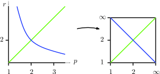
in illustrations has several advantages (see Figure 1). Firstly, we obtain finite pictures as is mapped onto . Moreover, the unreachably far away index becomes the handy point . The mapping preserves the order of the norm indices, i.e.
So, we are given just an appropriate scaling and the smallest possible index is of course the left-most point in the images. Last but not least, the index is mapped exactly to the middle of the line segment, befitting its special role as the only self-conjugate index.

As the first object of interest (2) involves two norm indices and we are going to use two-dimensional images by applying the scaling function twice independently:
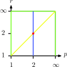
The result is a finite square whose center corresponds to the well known special case that was proved in [6]. There are some other nice side effects. The points satisfying still form a straight line in the graphics. Moreover, the curve is mapped to the square’s other diagonal (see Figure 2).
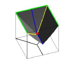
Later on, when we study (1) in full generality, we will use this same image scaling to three dimensional pictures:
There are again several curves that have lines as images. Furthermore, we will encounter some surfaces that are conveniently mapped to planes.
1.3 Basics on norm interpolation
We want to briefly introduce a concept that is a key to our proofs and will be used extensively in the remainder of the paper. More detailed explanations and additional applications can be found in [8].
In 1926 M. Riesz established a theorem that allows to interpolate between two inequalities involving the usual vector norms. Stated in our notations:
Theorem 1 (Riesz-Thorin)
Let and be given such that
| (3) |
If for a linear operator
| (4) |
there are such that
| (5) |
for all arguments , then for any and every vector the inequality
| (6) |
holds with defined by
| (7) |
The theorem was enshrined in the fundamental methods of analysis, when Riesz’ student G.O. Thorin extended the theorem to complex arguments and operators, obtaining an analogon of Theorem 1 with (4) replaced by
His proof, based on an ingenious use of Hadamard’s three line lemma from the theory of analytic functions, reveals the surprising fact that the condition (3) is no longer necessary in the complex case (essentially because condition (5) must now hold for all complex vectors); an assertion that is completely wrong in the real case!
Afterwards, the result was extended to operators defined on subspaces and, by help of density arguments, to operators acting on infinite-dimensional spaces, in particular the -spaces. Moreover, it was shown that, if and are matrices, the underlying norms may be replaced by their Schatten type analogues. This holds due to a general equivalence between sequence spaces and the corresponding Schatten classes as far as interpolation is concerned [1].
Recently, in [10], one of us restated the theorem in terms of a special structure, the tensor product of argument vectors, with the purpose of investigating (1) with . Although formulated in a more specific way in that paper, its wider validity was noted. Indeed, one can replace (4) by
and substitute
with matrices . That is, we are given a linear operator on the whole set of matrices, but only apply it to arguments that are tensor products (also called Kronecker product for matrices).
The proof is an adaption of Thorin’s proof as presented in [8], combined with the fact that the generated simple functions (actually vectors in the finite-dimensional case) respect the tensor structure of the arguments. As for the original theorem, and may be taken from subspaces of or , respectively.
In the aftermath of the WATIE 2009 conference we learned about the multilinear version of the Riesz-Thorin theorem. In the multilinear case (4) is replaced by the multilinear operator
(5) and (6) by inequalities like
Closer inspection revealed that the statement is actually equivalent to the usual interpolation but applied to tensor products, owing to the property of Schatten norms. Later on, we will see that the multilinear interpretation is too comprehensive for our needs, whereas the original interpolation theorem and its diagonal extension via tensor products serve their purpose very well. Be sure to read the acknowledgement for some more insights.
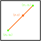
Our scaling function (Section 1.2) is especially convenient for picturing certain salient aspects related to norm interpolation. The Riesz-Thorin theorem, in particular (7), tells us that in terms of reciprocals, the interpolated index is a convex combination of the base indices and . This is the reason why the Riesz-Thorin theorem is sometimes called a convexity theorem.
If the norms of argument and target space are different (i.e. ), we need to consider a joint convex combination of the index reciprocals. Due to the way is defined in the images of this paper conveniently lies on a straight line between and .
We call the points interpolation base points and all points subject to (7) interpolants. We carry over this nomenclature to the associated inequalities and to the images of the points in our pictures.
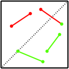
Note that for real interpolation both base points are necessarily located in the lower triangle determined by the main diagonal (Figure 3).
1.4 Overview
For the sake of clarity, in Section 2, we start with treating the original and simpler conjectured inequality (2), about the constant . Since only two parameters enter the treatment, the pictures are 2-dimensional. In Section 3, the approach used in Section 2 is generalised to treat as much of the general 3-parameter problem as possible. In the course of this process, we will encounter a number of parameter regions that could not, as yet, be treated using the interpolation methods applied in Section 2. To overcome this hurdle, two things are needed. Firstly, the value of in certain extremal points of parameter space must be established. This is done in Section 4 using a combination of basic linear algebra methods and esoteric knowledge about certain magical symbols. Secondly, the remaining areas of parameter space have to be covered, and this is done in Section 4.3 using more advanced versions of Riesz-Thorin interpolation. Thus, the proof of our main theorem is finished at that point. We hasten to add that for certain areas in parameter space the constant depends on the dimension of the matrices. Furthermore, in some instances the interpolation method did not yield the sharpest possible bound. In Section 5, the cases of equality are considered, and we wrap up with a conclusion (Section 6) and a list of recommended readings.
2 The original conjecture and its proof
This section is dedicated to the derivation of (2), which is the following theorem.
Theorem 2
With the notations of equation (1),
This is the original conjecture stated in [2]. The proof we give here is somewhat longer than what could have been, but in this way it clearly demonstrates the power and applicability of interpolation. Near the end of this section, the reader will notice that the proof may be shortened a bit.
2.1 The claim and some special situations
To begin with, we ensure that the value claimed for can be attained. For this, take a look at the examples
| (8) |
yielding the quotients as well as and
| (9) |
giving the value . Hence, the constant cannot be smaller than asserted.
Because of the appearance of a maximum, over the three terms as stated in Theorem 2, the set of all pairs of norm indices is naturally subdivided into three segments:
That this is an equivalent statement is easily verified analytically and is illustrated in Figure 4.
The conjecture is already known to be true in some special cases, namely

2.2 A re-interpretation of known cases
First we reconsider the case , but from a different point of view. The validity was obtained by one of us as a consequence of an even stronger inequality [2]. We want to deduce the value of in a different way, show-casing the two major techniques (complex interpolation and norm index monotonicity, see below) we will repeatedly use in the rest of the paper.
We will also demonstrate the strong link between the promised pictures and the associated argumentation and formulas.
[l]![[Uncaptioned image]](/html/1004.2700/assets/x9.png) \picskip7
We know the values of and from the inequalities
\picskip7
We know the values of and from the inequalities
for all matrices and . The respective pairs of parameter values and are represented by the green points in the picture at the left.
Now fix an arbitrary with and consider the commutator as a linear operator
Clearly, we have
for any . As these correspond to the premises (5) of the Riesz-Thorin theorem, in its usual form, (see Theorem 1 and the comments on generalization thereafter) we endeavour to apply this theorem for (the points on the orange line in the picture). For this we require the validity of (7), which is, in our case: for any
As the first equality is trivially true we have that the parameter
is in one-to-one correspondence to all possible interpolants . Consequently, we obtain inequality (6), that is
or equivalently
and hence , as required. Note that assuming to be normalised incurs no loss of generality.
[l]![[Uncaptioned image]](/html/1004.2700/assets/x10.png) \picskip8For the remaining case we can use a simpler concept,
which we would like to call norm index monotonicity, or just monotonicity for short. By this
we mean the well-known relation
\picskip8For the remaining case we can use a simpler concept,
which we would like to call norm index monotonicity, or just monotonicity for short. By this
we mean the well-known relation
and arbitrary matrices . This procedure could be regarded as an interpolation with only one base.
In this manner we obtain directly from the knowledge of that
which gives for (points on the yellow line).
For both cases, and , the proof is now easily completed by providing an example of two matrices that achieve equality, as we have already done in Section 2.1.
We will keep on the arrangement for picturing known base points green and indicating an interpolation process by an orange line and the use of the monotonicity argument by a yellow line.
2.3 Towards a full proof
In this section we give an intuitive overview of the proof of Theorem 2, but on the other hand also provide the necessary details for more demanding readers. To accommodate both audiences we have adopted an unusual style that may be called a scientific graphic novel. In an attempt to avoid boring the reader too much, the level of detail will be reduced in due course when coming across cases that are similar to already covered ones.
Roughly speaking, the proof can be subdivided in four parts, each part corresponding to one of the four quadrants of the parameter space: the lower left quadrant, corresponding to , the lower right, , , the upper right , and the upper left quadrant , . We begin with the lower left quadrant.
[l]![[Uncaptioned image]](/html/1004.2700/assets/x11.png) \picskip8
The conjecture can easily be shown to be true for by ordinary Riesz-Thorin interpolation.
For this fix arbitrarily.
\picskip8
The conjecture can easily be shown to be true for by ordinary Riesz-Thorin interpolation.
For this fix arbitrarily.
We obtain two points on the green lines in the picture, for which we have
Regard the commutator as a map with some fixed with . So,
As the norm indices of original and target space coincide for both inequalities, we need to satisfy
twice. Hence, and from the Riesz-Thorin theorem we immediately get .
[l]![[Uncaptioned image]](/html/1004.2700/assets/x12.png) \picskip6
Interpolation also works in the case . Again,
fix . Here, we have
\picskip6
Interpolation also works in the case . Again,
fix . Here, we have
Interpolation of now requires
which amounts to and yields .
Note that applicability of Theorem 1 comes from fixing the variable (for given norm index ) or (for given , as in the last subsection), which is expressed by a vertical or horizontal line in our graphics of norm index pairs . We remark that jointly interpolating and for bivariate inequalities is not supported by the original theorem. Hence, slanted (non-horizontal, non-vertical) lines for interpolation are forbidden here.
[l]![[Uncaptioned image]](/html/1004.2700/assets/x13.png)
![[Uncaptioned image]](/html/1004.2700/assets/x14.png) \picskip6
Now, having covered half of the proof, interpolation will not work for
as it did in the previous cases.
Regardless whether we interpolate (left) or (right), i.e. fixing or , the
obtained bound always gives a larger value than the one claimed in Theorem 2:
.
See Figure 6 for an illustration of the difference.
\picskip6
Now, having covered half of the proof, interpolation will not work for
as it did in the previous cases.
Regardless whether we interpolate (left) or (right), i.e. fixing or , the
obtained bound always gives a larger value than the one claimed in Theorem 2:
.
See Figure 6 for an illustration of the difference.
[l]![[Uncaptioned image]](/html/1004.2700/assets/x15.png)
![[Uncaptioned image]](/html/1004.2700/assets/x16.png) \picskip6
Analogously, for , interpolation does not yield the desired bound either, but gives
the larger value of .
\picskip6
Analogously, for , interpolation does not yield the desired bound either, but gives
the larger value of .
This actually was to be expected, since interpolation produces smooth bounds, while the claimed constant
is not smooth as function of and .
To wit, the graph of the constant exhibits cusps at the lines and , lines that are intersected
by the current directions of interpolation; for this reason we call these lines cusp lines.
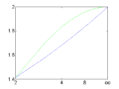
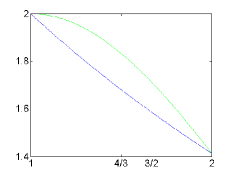
Nevertheless, we can obtain sharp values for in a more complicated, two-step interpolation process, combining one of the more advanced versions of the Riesz-Thorin method with its ordinary version, and carefully choosing the right step at the right time.
[l]![[Uncaptioned image]](/html/1004.2700/assets/x19.png) \picskip6
The value of along one of the cusp lines, namely the main diagonal ,
can be obtained with help of the tensor structure interpolation
mentioned in Section 1.3, between and .
By applying the usual interpolation
statements on these special arguments, interpolation along diagonal lines becomes possible.
This has already been done in [10], with the result
for (and for ).
\picskip6
The value of along one of the cusp lines, namely the main diagonal ,
can be obtained with help of the tensor structure interpolation
mentioned in Section 1.3, between and .
By applying the usual interpolation
statements on these special arguments, interpolation along diagonal lines becomes possible.
This has already been done in [10], with the result
for (and for ).
Note that for
this result has also been obtained in the above, but in a single step, using ordinary
Riesz-Thorin interpolation.
This shows that the more complicated approach does not always lead to sharper bounds.
[l]![[Uncaptioned image]](/html/1004.2700/assets/x20.png) \picskip8
Instead of interpolating over the whole upper right quadrant we can now
do this in a triangle only, and get sharp values, exhibiting the cusp at the diagonal.
Fix .
We have
\picskip8
Instead of interpolating over the whole upper right quadrant we can now
do this in a triangle only, and get sharp values, exhibiting the cusp at the diagonal.
Fix .
We have
and consider . By
and consequently we get , as claimed.
[l]![[Uncaptioned image]](/html/1004.2700/assets/x21.png) \picskip8
Similarly, for the second triangle, fix . We know the bounds for
the two base points:
\picskip8
Similarly, for the second triangle, fix . We know the bounds for
the two base points:
Now, by interpreting the commutator as the linear map we obtain
or and .
[l]![[Uncaptioned image]](/html/1004.2700/assets/x22.png)
![[Uncaptioned image]](/html/1004.2700/assets/x23.png) \picskip6
We ought to remark that it is easier to interpolate the two triangles along the other respective direction
(i.e. fixing the other variable as we have done above), as the
constant in the corresponding inequalities is the same for both interpolation base points
and, hence, automatically yields exactly this value for all interpolant inequalities.
We don’t even need to determine the relation linking the parameter with or .
Note that this only works because some of the base points were determined before by other interpolation
steps, whereas the variant given first relies only on the trivial estimates on the boundary
of the square.
\picskip6
We ought to remark that it is easier to interpolate the two triangles along the other respective direction
(i.e. fixing the other variable as we have done above), as the
constant in the corresponding inequalities is the same for both interpolation base points
and, hence, automatically yields exactly this value for all interpolant inequalities.
We don’t even need to determine the relation linking the parameter with or .
Note that this only works because some of the base points were determined before by other interpolation
steps, whereas the variant given first relies only on the trivial estimates on the boundary
of the square.
[l]![[Uncaptioned image]](/html/1004.2700/assets/x24.png) \picskip6
In the last, upper left quadrant, another cusp line appears. In order to proceed
in a similar way as we did with the upper right quadrant, the anti-diagonal is needed.
Fortunately we can obtain these values by a simple duality argument, as follows.
For we have
\picskip6
In the last, upper left quadrant, another cusp line appears. In order to proceed
in a similar way as we did with the upper right quadrant, the anti-diagonal is needed.
Fortunately we can obtain these values by a simple duality argument, as follows.
For we have
obtained from tensor product interpolation (green line). Then for any with one has
We conclude
giving for , which is the assertion for the anti-diagonal (red line); see the proof of Proposition 4 for details on the above equality.
[l]![[Uncaptioned image]](/html/1004.2700/assets/x25.png)
![[Uncaptioned image]](/html/1004.2700/assets/x26.png) It should be clear now that in complete analogy to the upper right quadrant we have to
interpolate the two triangles separately. Again it doesn’t matter along which direction
we fix one of the norm indices.
It should be clear now that in complete analogy to the upper right quadrant we have to
interpolate the two triangles separately. Again it doesn’t matter along which direction
we fix one of the norm indices.
[l]![[Uncaptioned image]](/html/1004.2700/assets/x27.png)
![[Uncaptioned image]](/html/1004.2700/assets/x28.png) \picskip6
Of course, one of the directions is easier than the other.
We leave it to the reader
to find out which one is preferable.
\picskip6
Of course, one of the directions is easier than the other.
We leave it to the reader
to find out which one is preferable.
We skip the details as the result does also follow from a plain duality argument
(as we have done for the anti-diagonal). By this argument we directly get
, which may be interpreted as a reflection symmetry of the constant about the line .
2.4 A little short-cut
[l]![[Uncaptioned image]](/html/1004.2700/assets/x29.png)
![[Uncaptioned image]](/html/1004.2700/assets/x30.png) \picskip6
The case and similarly can be done in an even easier way using norm index monotonicity.
By this, the value (known for points on the green line in the left picture)
extends to all .
So, after the diagonal interpolation (as the really first step), this attempt may replace the previous investigations
of the lower right quadrant and one triangle. Similarly, once we obtain the anti-diagonal by duality, the observations for the
lower left quadrant follow automatically.
\picskip6
The case and similarly can be done in an even easier way using norm index monotonicity.
By this, the value (known for points on the green line in the left picture)
extends to all .
So, after the diagonal interpolation (as the really first step), this attempt may replace the previous investigations
of the lower right quadrant and one triangle. Similarly, once we obtain the anti-diagonal by duality, the observations for the
lower left quadrant follow automatically.
[l] ![[Uncaptioned image]](/html/1004.2700/assets/x31.png) Also note that the remaining two single triangles can be merged into a single step. This cannot be done
with help of the norm index monotonicity, and interpolation (with fixed ) becomes necessary.
However, since both base inequalities admit the same constant, this turns out to be pretty easy.
Also note that the remaining two single triangles can be merged into a single step. This cannot be done
with help of the norm index monotonicity, and interpolation (with fixed ) becomes necessary.
However, since both base inequalities admit the same constant, this turns out to be pretty easy.
[l] ![[Uncaptioned image]](/html/1004.2700/assets/x32.png) \picskip6
Finally, we remark that the diagonal tensor interpolation, the dual anti-diagonal values
and the triangle interpolation between both can also be merged into a single step
by applying the multilinear extension of the Riesz-Thorin theorem.
However, we will not give more details about this since the treatment
of (7) requires the synchronization of three equalities
and the calculation of the value of the interpolated bound is no longer that easy.
\picskip6
Finally, we remark that the diagonal tensor interpolation, the dual anti-diagonal values
and the triangle interpolation between both can also be merged into a single step
by applying the multilinear extension of the Riesz-Thorin theorem.
However, we will not give more details about this since the treatment
of (7) requires the synchronization of three equalities
and the calculation of the value of the interpolated bound is no longer that easy.
3 Generalisation
In the previous section we have proven Theorem 2, which is really a special case of inequality (1). In the present section we want to try our two main tools, as well as some slightly more delicate things, to see how much extra mileage they allow us on the road towards a full proof of inequality (1). In that sense, this section is really a continuation of Section 2. The main result of these investigations can be found at the end of this section.
[l]![[Uncaptioned image]](/html/1004.2700/assets/x33.png) \picskip10
For the general situation (1) three norm indices and
have to be depicted, requiring three-dimensional images.
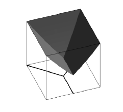
In what follows, we transform the cube by the mapping
and represent its image using a perspective projection from a fixed viewing direction.
Under these circumstances we can again drop axis labels, just as in Section 2.
Note that is again represented by the cube’s center (red point).
\picskip10
For the general situation (1) three norm indices and
have to be depicted, requiring three-dimensional images.
In what follows, we transform the cube by the mapping
and represent its image using a perspective projection from a fixed viewing direction.
Under these circumstances we can again drop axis labels, just as in Section 2.
Note that is again represented by the cube’s center (red point).
As of now, regions of parameter space will be colored differently depending on the rule that determines .
[l]![[Uncaptioned image]](/html/1004.2700/assets/x34.png)
![[Uncaptioned image]](/html/1004.2700/assets/x35.png) \picskip11
First, we picture the (now proven) originally conjectured special case in the general context. We know the values of
\picskip11
First, we picture the (now proven) originally conjectured special case in the general context. We know the values of
and by swapping the roles of and also of
[l]![[Uncaptioned image]](/html/1004.2700/assets/x36.png) \picskip11
These constants are represented by triplets on the planes and .
Due to the properties of our scaling function the latter are indeed planes
(recall similar statements for given in Section 1.2).
\picskip11
These constants are represented by triplets on the planes and .
Due to the properties of our scaling function the latter are indeed planes
(recall similar statements for given in Section 1.2).
We combine the two results and moreover modify them in a way
that turns out to be more suitable for what follows.
Naturally, one has and
in the two planes, respectively.
3.1 Monotonicity conquers (almost) all
The validity of the conjecture naturally extends to some of the cases with , by applying the norm index monotonicity argument.
[l]![[Uncaptioned image]](/html/1004.2700/assets/x37.png)
![[Uncaptioned image]](/html/1004.2700/assets/x38.png) First take a look at triplets connected to the constant . This value
does not depend on and . So, we choose some point on the pictured segment
in the left image. We obtain, for all ,
First take a look at triplets connected to the constant . This value
does not depend on and . So, we choose some point on the pictured segment
in the left image. We obtain, for all ,
for arbitrary matrices and . Moreover, for points as in the right image we get
for any .
![[Uncaptioned image]](/html/1004.2700/assets/x39.png)
![[Uncaptioned image]](/html/1004.2700/assets/x40.png)
![[Uncaptioned image]](/html/1004.2700/assets/x41.png)
![[Uncaptioned image]](/html/1004.2700/assets/x42.png)
For triplets belonging to we may argue in an analogous way for any (left) and also for any (right).
As we only obtain upper bounds, we also need an example achieving equality. One such is given by (8). Note that matrices of rank one are essential for achieving equality in monotonicity relations. We will treat this in more detail later.
Similarly, for the segment where the constant is , which is independent of and , one can extend the bound to (left) and (right). Taking into account (9) we see that the value is sharp in these areas.
[l]![[Uncaptioned image]](/html/1004.2700/assets/x43.png)
Summing up the results obtained so far, we get that the constant of Theorem 2 is valid also for a huge part of the general setting, namely for all with or , but not with all of and . Here we have one more indication that the areas (like the processes) are a lot easier to visualize than to capture in formulas.
We point out the reflection symmetry of the areas and their values. The light blue area is the image of the dark blue area under reflection about the plane , and the pink area is symmetric about that plane. One can even check that the value of equals the value in its mirror point. This symmetry originates from the symmetry of under interchanging both with , and with , as will be discussed in more detail at the end of this section (Proposition 4).
3.2 Some more sophisticated techniques
[l]![[Uncaptioned image]](/html/1004.2700/assets/x44.png) \picskip9
For the next steps we need the values for points . These
can be obtained by a Hölder-type inequality which is true for
Schatten norms
\picskip9
For the next steps we need the values for points . These
can be obtained by a Hölder-type inequality which is true for
Schatten norms
whence, combined with the triangle inequality, one has giving . Example (9) shows that equality can be achieved.
[l]![[Uncaptioned image]](/html/1004.2700/assets/x45.png)
Now take any point from the line we just observed and apply the monotonicity tool once more. We get for all .
Example (9) again achieves equality here, and the whole triangle admits the value 2.
The points in the triangle then serve as base points for the next interpolation step.
\parpic
[l]![[Uncaptioned image]](/html/1004.2700/assets/x46.png)
![[Uncaptioned image]](/html/1004.2700/assets/x47.png) \picskip10
Choose and arbitrarily in the grey triangle. We are going to interpolate only
between 1 and (if , left picture) or 1 and (if , right picture).
For example, for the first case one has for (7)
\picskip10
Choose and arbitrarily in the grey triangle. We are going to interpolate only
between 1 and (if , left picture) or 1 and (if , right picture).
For example, for the first case one has for (7)
which yields
Note that it doesn’t matter whether we interpolate or , as both and are fixed.
[l]![[Uncaptioned image]](/html/1004.2700/assets/x48.png) \picskip11
For the second case we may proceed in an analogous way, or alternatively rely on the --symmetry
already mentioned at the end of Section 3.1.
\picskip11
For the second case we may proceed in an analogous way, or alternatively rely on the --symmetry
already mentioned at the end of Section 3.1.
Also note that the area connected to is now of the same shape as the areas
of and .
By this, we obtain two more symmetry planes, which are investigated in detail in Proposition 4,
and which ensure the symmetry of the values and not only of the area’s shape.
[l]![[Uncaptioned image]](/html/1004.2700/assets/x49.png) \picskip9
Our next aim is to close the mould formed by the three areas for which the constant is known so far.
First we interpolate between the two points and .
Both of them admit the constant 2, hence the points inbetween all share
this value.
The only remaining task is to determine which are the points inbetween.
Since is fixed, simple interpolation will work and requires
\picskip9
Our next aim is to close the mould formed by the three areas for which the constant is known so far.
First we interpolate between the two points and .
Both of them admit the constant 2, hence the points inbetween all share
this value.
The only remaining task is to determine which are the points inbetween.
Since is fixed, simple interpolation will work and requires
Combining the latter we obtain the value 2 for all points satisfying
We remark that maps the set of these triplets to a planar triangle. After having done this calculation one gets an impression of the difficulties involved in the multilinear version, when three equations come into play.
[l]![[Uncaptioned image]](/html/1004.2700/assets/x50.png)
![[Uncaptioned image]](/html/1004.2700/assets/x51.png) \picskip9
Now we are in a position to close the gap between the plane that we have treated
and the known bodies, by means of interpolation. For this, again fix and
as only will vary. Now choose such that .
Hence, lies in the brown triangle. The appropriate base point in the light blue
triangle is then given by (left image). For interpolants we
need to satisfy
\picskip9
Now we are in a position to close the gap between the plane that we have treated
and the known bodies, by means of interpolation. For this, again fix and
as only will vary. Now choose such that .
Hence, lies in the brown triangle. The appropriate base point in the light blue
triangle is then given by (left image). For interpolants we
need to satisfy
which results in the bound
While this value seems to be rather exotic and maybe even perplexing it is sharp nonetheless, as demonstrated by the example
| (10) |
The second case is again done in a similar way or obtained by the --symmetry.
3.3 Trouble…
Knowledge of the constants for the plane successfully helped to obtain the values in a triangular pyramid. So it is natural to try the same for the pyramid opposite to it. In order to perform the interpolation we need the value of the pyramid’s top. Unfortunately, this value is no longer independent of the matrix size . Thanks to the well-known inequalities
| (11) |
we find a simple upper bound given by .
Using techniques similar to those used in the last section, one gets the upper bound
This follows in three steps: interpolating the line , the plane
![[Uncaptioned image]](/html/1004.2700/assets/x52.png)
![[Uncaptioned image]](/html/1004.2700/assets/x53.png)
![[Uncaptioned image]](/html/1004.2700/assets/x54.png)
and finally the pyramid .
At this point the interpolation method runs out of steam. Whereas for even the value is shown to be sharp by the example
with matrices and as in (10), we are unable to find an example when is odd. The reason may be that in this case the estimate (11) is already not sharp.
[l]![[Uncaptioned image]](/html/1004.2700/assets/x55.png) \picskip10
The last area not yet investigated is the cube given by and .
We do know the value of for three of its facets, namely .
The obvious method to apply is monotonicity. For instance, as indicated in the picture
we may write
\picskip10
The last area not yet investigated is the cube given by and .
We do know the value of for three of its facets, namely .
The obvious method to apply is monotonicity. For instance, as indicated in the picture
we may write
for any . By this, the upper bound is extended to the whole cube. Of course, one can use the monotonicity argument also with reducing or based on the other facets instead.
Sadly, this value is not sharp, and we can show this as follows. First we observe that the value is obtained solely by the knowledge of , as the values on the facets themselves followed from the value at the point using monotonicity. Now, we can use the fact that for equality in holds if and only if . Hence, applying this for all indices, we see that , and must all be matrices of rank one satisfying the equality . From Proposition 4.5 of [6] we know that without loss of generality two rank one matrices and satisfy this equality only if there are vectors such that and . However, under those conditions, has rank two, yielding a contradiction.
3.4 The result, so far
The previous steps obtained in this section (that is, the positive ones) add up to the following theorem.
Theorem 3
For with , excluding the octant and , one has
The four segments of corresponding to each of the four arguments of the maximum function are given as follows:
![[Uncaptioned image]](/html/1004.2700/assets/x56.png)
when
, ,
and
;
when
, ,
and
;
![[Uncaptioned image]](/html/1004.2700/assets/x57.png)
![[Uncaptioned image]](/html/1004.2700/assets/x58.png)
when
, ,
and
;
when
,
,
and .
![[Uncaptioned image]](/html/1004.2700/assets/x59.png)
For matrices of even size and with one has
If is odd the latter is only an upper bound.
![[Uncaptioned image]](/html/1004.2700/assets/x60.png)
Note that the constant for parameters in the region (i.e. the first four cases of Theorem 3) are independant of dimension. Hence, the statement is also true in the infinite-dimensional setting of Schatten norms.
The following result summarises all the symmetries we have encountered and also encapsulates the duality arguments mentioned at the end of Section 2.3.
Proposition 4
For any one has
These three equalities represent the reflection symmetries of about the planes , , and , respectively:
![[Uncaptioned image]](/html/1004.2700/assets/x61.png)
![[Uncaptioned image]](/html/1004.2700/assets/x62.png)
![[Uncaptioned image]](/html/1004.2700/assets/x63.png)
The third picture generalises the duality statement from Section 2.3.
Proof. The first equality is a mere consequence of and the resulting possibility of changing the roles of and .
Now for the second equality, observe that for any fixed with
and imply the assertion. Here, denotes the inner product associated with the Schatten classes. The third equality is analogous or can be proved by combining the first two equalities. \qed
The representations of norms as given in the last proof are called variational characterisations and they will be of extraordinary use in the following section, too.
4 Extremal points
In the previous section we have squeezed the last drop out of the interpolation, monotonicity and duality methods, but two areas in parameter space, a tetrahedron and a cube, still resist treatment. In the present section we finally tackle these recalcitrant areas by finding the value of the constant in two specific points. To do so, some new ideas are needed.
4.1 The skeleton
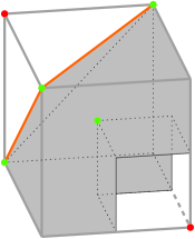
In Figure 7 we depict all constellations covered so far in Sections 2 and 3 by marking them in grey. All the values of the constant in these triplets were the result of the knowledge of its value in only four points (or three, using symmetry), namely and or (marked green). We also relied on the values of the points on the orange lines. However, a closer look reveals that these may be obtained from interpolation between two of the four green base points, too.
In Section 3.3 we had a quick glance at the remaining two areas (white). In one situation, monotonicity failed, while in the other the value at the interpolation base point was likely not well-estimated (at least for odd-sized matrices).
In any case, the natural approach for carrying this further is to find the exact value of the constants ( odd) and . These are the triplets marked red in the figure.
4.2 The value of the constant at the corners
In this subsection we provide the value of the constant in the two corners just mentioned. We prove the following theorem:
Theorem 5
For matrices one has
-
a)
-
b)
.
Proof of a).
We only need to prove the formula for odd , as the value for even was already shown in Section 3.3 in a much easier way. However, as it requires no extra efforts, we nonetheless prove that particular result again in the same fashion as for the odd case.
A variational characterisation for is given by
Let us first fix . The function to be maximised is convex in , and the feasible set of is convex as well, with extremal points given by the set of unitary matrices. Thus, we can write:
A similar argument allows to conclude that can also be restricted to the set of unitary matrices:
In addition, the trace norm has a variational characterisation as well:
Thus we get a maximisation over three unitary matrices:
Every unitary matrix is unitarily equivalent to a diagonal matrix with all diagonal elements of modulus 1. Applying this to , we get
The matrix can be absorbed into and , so that w.l.o.g. we can restrict to be of this diagonal form. Indeed,
where and .
Then can be rewritten as a Hadamard product: , with a matrix with entries . The function to be maximised becomes
The Cauchy-Schwartz inequality leads to a further upper bound:
Applying the maximisation over all unitary and to both sides then yields
because both factors of the right-hand side could be maximised separately, and both maxima are equal. Now note that the matrix with elements is a doubly stochastic matrix (because is unitary). Furthermore, the function to be maximised is linear in . Hence, the maximum is achieved in extremal points of the set of doubly stochastic matrices. By Birkhoff’s theorem [5], these are permutation matrices. Thus we have a further reduction:
where the maximum is over all permutations . Observe that this inequality is actually an equality, as the left-hand side attains the right-hand side for and both equal to the permutation matrix representing .
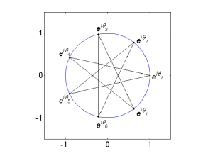
We are now left with calculating the maximum over all angles and all permutations of . This problem has a nice geometric interpretation. The complex numbers are points on the unit circle. The permutation maps every point to another point, in a one-to-one fashion. If we draw edges from to we obtain one or more polygons (in general, non-convex and self-intersecting), corresponding to the cycles of the permutation. The problem is to distribute the points on the circle and choose the polygons so that the total length of the edges (the total circumference of the polygon(s)) is maximised.
For even , the maximum is easy to find: points are equal to 1 while the others are , and the permutation consists of 2-cycles. The maximum length is therefore . See Figure 8 for an illustration. The odd case is not that simple. Whereas can still easily be seen, larger sizes are more difficult. It turns out that the maximal length is obtained when is a cyclic permutation (so that we have only one polygon), the points are the -th roots of unity, and they are connected in the shape of a star polygon with Schläfli-symbol (see Figure 9). The upshot is that there are edges, and every edge has the same length .
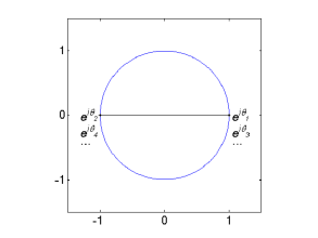
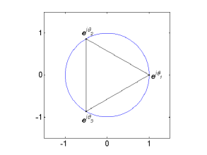
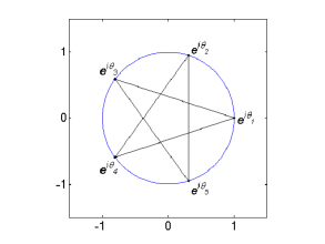
We will prove this in two steps. First we calculate the maximal circumference of a single -polygon (corresponding to being cyclic). Second, we show that is superadditive: . That is, the total circumference does not increase by using a permutation consisting of several, shorter cycles.
We first maximise over all angles for a cyclic permutation. As we can relabel the angles, it does not matter which cyclic permutation we take. It therefore suffices to maximise , with , which is equal to . Define , so that . We can now replace the maximisation over the angles by a maximisation over their differences , with the condition that should be an integer multiple of (because of the cyclicity of ). Noting also that , which in turn is equal to over the interval , we then have the constrained maximisation
From the concavity of the sine function over the interval , we get
with equality if all are equal. Therefore, the maximisation over the is readily done, and we get
The remaining maximisation over is also easy: for even , (with ), while for odd we get the smaller value
It remains to prove superadditivity of , i.e.
For even , this is simple: either and are both even, in which case , or they are both odd, in which case .
For odd , consider odd and even, so that . We note that for odd is an increasing function of . Hence for odd and , , which directly implies . This ends the proof of a).
Proof of b). A variational characterisation of is
Now note that is convex in , and that the set of such that is a convex set with extremal points the rank 1 matrices , where and are normalised vectors. Thus,
is achieved for of the form .
Similarly, the latter is a convex function in (the pointwise maximum of two convex functions is again convex) and, therefore, is also maximal for of the form , where and are normalised vectors. Hence,
The norm itself also has a variational expression:
where and are also normalised vectors. We thus end up with a maximisation over 6 normalised vectors:
It is in principle possible to perform this maximisation over each of the 6 vectors in turn, but the calculations immediately become very long-winded. A much better approach is to focus attention to the inner products directly.
W.l.o.g. we can restrict the values of all inner products to be real, which can be done simply by considering real vectors only. It is easily seen that cannot be made bigger by allowing complex valued inner products. Thus, let , and , and , and . The point to observe now is that of these angles exactly 5 can be chosen independently, while the remaining one is then subject to an inequality, as illustrated here:
In this example, , the angle between and , is restricted to be less than the sum of all other angles (which is not a restriction if that sum is larger than ). Thus we get
Lemma 6
and
Lemma 7
For ,
For ,
The maximal and minimal values outside these intervals are obtained by periodical extension.
Proof of Lemma 7. By applying Lemma 6, we get
The stationary points of as function of are and , yielding the values and . The maximum of these values is for , while the maximum outside this interval is obtained by periodical extension. The minimum is calculated in a similar way. \qed
With this lemma we are thus led to replace the maximisation over the 6 angles by a single maximisation: we maximise the first term over angles subject to , and minimise the second term over angles subject to (as the sign of and is irrelevant in we can use Lemma 7 here too). This leads to
The maximum is achieved for and equal to . This ends the proof of b). \qed
4.3 Interpolation revisited
The major hope behind Theorem 5 is of course that we might be able to use interpolation to close the two gaps for the unknown triplets .
[l]![[Uncaptioned image]](/html/1004.2700/assets/x69.png) \picskip8
For (the cube in the lower right of the illustrations) interpolation turns out
to be the wrong method, at least with the present data. We demonstrate this for the line .
Even the exact value of does not force interpolation bounds
to be sharp in this case.
We obtain
\picskip8
For (the cube in the lower right of the illustrations) interpolation turns out
to be the wrong method, at least with the present data. We demonstrate this for the line .
Even the exact value of does not force interpolation bounds
to be sharp in this case.
We obtain
| (12) |
However, as in the proof of Theorem 5 b) one can show that for these points the and achieving the maximum are matrices of rank one. Hence, has at most two non-zero singular values. Combining the knowledge of
| : | and | |
|---|---|---|
| : |
already yields a better upper estimate than (12), in fact
| (13) |
Recalling the example (9) given in Section 2.1 we may ensure
| (14) |
Alas, this is a worse lower bound for as it tends to .
The trickier example of two (normed) rank one matrices from [6, page 1880] gives us the curve
| (15) |
for possible singular values of .
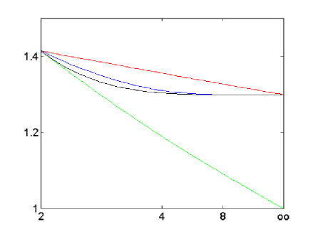
By choosing a point on the curve (15) with -norm as large as possible we obtain a very good lower bound to , which is numerically approximated in Figure 10. Moreover, we conjecture that the resulting value is equal to the constant for . The estimates given by the upper and lower bounds (also pictured in the figure) are already very tight.
Note that and can be determined by duality from . Recall the symmetries of Proposition 4 for that purpose.
[l]![[Uncaptioned image]](/html/1004.2700/assets/x71.png) \picskip7
Similarly, for odd-sized matrices in the upper left pyramid there seems to be one more
plane of cusps determined by the example used for in Theorem 5 a)
\picskip7
Similarly, for odd-sized matrices in the upper left pyramid there seems to be one more
plane of cusps determined by the example used for in Theorem 5 a)
yielding the value
| (16) |
on the one hand, as well as the value
| (17) |
on the other hand, given by padding an example matrix of even size with a zero line and column
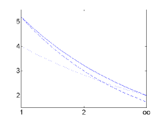
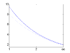
In the picture we indicated the areas of the pyramid where the examples yielding (16) or (17) represent the largest known lower bounds. Assuming that these two values are equal to and that the two examples achieve the pyramid’s values, it is left as a simple exercise in interpolation to show that the interface boundary surface is really mapped to a plane by . The second example is indeed a direct sum of the matrices (10) from Section 3.3, padded with an additional row and column of zeroes to get an odd dimension; recall that for even dimension these matrices did achieve equality.
The interpolation bound
| (18) |
is likely not sharp.
5 Maximality
In [6], after giving the first general proof for , the notion of maximality was introduced. This notion was subsequently extended to -maximality in [10]. Consistent with these definitions we want to investigate the maximality problem in the general context and call a pair of matrices -maximal if both and are non-zero and satisfy (1) with equality, i.e.
In contrast to [10], we are only looking here at the Schatten norms.
A characterization of -maximality, which is called maximality in [6] and Schatten 2-maximality in [10], was recently given in [7]. This result will serve as a basis for further investigations to derive criteria for maximality in the case, in combination with the tools we have used in Sections 2 and 3 to obtain the exact values of the bound .
First of all, we will see that the method of monotonicity imposes strong restrictions.
Lemma 8
-
a)
If was obtained by monotonicity via increasing and is -maximal then and is -maximal.
-
b)
If was obtained by monotonicity via decreasing and is -maximal then and is -maximal. An analogous statement is true for and .
Proof. The monotonicity argument in a) works as follows:
Hence, if is -maximal, the left-hand side equals and this implies the -maximality of the pair since all of the inequalities in the chain become equalities. Moreover, we get
for which is only possible if the corresponding matrix has rank one.
The proof of b) is similar. \qed
In [10] we argued that some properties are preserved by interpolation. Furthermore, we used the fact that especially a rank one structure is left untouched. Of course, this argument only works if the obtained interpolation bounds are sharp.
Lemma 9
Let .
-
a)
If is obtained by interpolation connected to a base, for which all matrices of a maximal pair admit rank one, then also the matrices of a -maximal pair must have rank one. Similar statements hold for and .
-
b)
If is obtained by interpolation between any point and (directly or via several steps) and is -maximal then is -maximal.
-
c)
If is obtained by interpolation connected to a base, for which all matrices of a maximal pair are unitarily similar to matrices of the type with , then also all matrices of a -maximal pair have this property. Similar statements hold for and .
Proof. The key point in the proofs is that if is a maximal pair with respect to an interpolated triplet, then an appropriately modified pair is maximal with respect to the base point triplet.
An analysis in [10, proof of Proposition 8] showed that the matrix is actually a scaled version of in the sense that every entry (i.e. a complex number) keeps its complex argument, but has its absolute value raised to a specific power (one of us calls this operation a polar power; see [3]). More precisely, if then .
Clearly, an entry with the value 0 is not altered in any way by this procedure. Moreover, the claim of a) was already proven true and applied in [10] based on these ideas.
Now, for any interpolation connected to the base point or any other point that has been obtained by such a process, the scaled pair needs to be maximal in the original sense. This statement is true if the interpolation process is the usual Riesz-Thorin theorem (complex version) or the tensor argument extension, since the tensor structure is unharmed by the scaling procedure.
The only information that we had obtained in [6] about matrices of a maximal pair was that they should have rank at most two, which was not enough to obtain meaningful restrictions for interpolants in [10]. But with the simultaneous unitary similarity to essentially matrices, it is now easy to see that with also is given. The last conclusion is only possible as the trace is now the sum of only two entries, or equivalently we have the relation
which is kept by scaling the modulus back to .
For transferring the orthogonality of and to and we furthermore need the well-known statement that a trace zero matrix is unitarily similar to a matrix whose diagonal elements are all zero ([9], p. 77). Hence, without loss of generality we may assume , implying for the scalar product
Of course, the latter is also preserved by scaling, since there are again only two summands in which exactly one component of and one of appear as factors. Since obeys the same relations as specified above and the theorems in [7] yield necessary and sufficient conditions, we obtain the -maximality of the pair.
The claim of c) can be shown in a similar but even simpler fashion. \qed
Remark. The part c) in Lemma 9 is a generalization of a) since every rank one matrix with trace zero is unitarily similar to a matrix of the type . The zero trace will automatically be given in combination with b). Note that for the described type of matrices one has for some . Hence, is unitarily similar to a multiple of a unitary matrix that is padded with zeros.
As all matrices of maximal pairs connected to b) admit rank not greater than two, we are able to apply the strong estimate
for Schatten norms. In general, the constant 2 in the second inequality would have been the rank or even the size . Such estimates were crucial in [10] to determine -maximal pairs and will also be of use in the following.
Both Lemmas imply that maximal pairs can only be found in a very limited range. We will see that only the boundary of the parameter space may need a separate treatment, but will mostly fit with the results of the interior. Lemma 9 b) implies that moreover -maximality can be expected to be richer than others (excluding possibly cases like at the boundary). Before proceeding with the consequences of these two results we need to introduce a new drawing convention we’ll adhere to.
Up to now we had no problems to picture sets of points , as all of them were closed sets, i.e. points, lines with end-points or complete bodies containing all of its bounding facets. However, for visualizing areas connected to shared properties of maximality we will encounter open sets. In order to visualize them in a comprehensible way we only draw lines and points instead of colored facets, and in the following way:
This marks all points on the line except the right end.
This picture marks all points of the triangle, excluding the grey edge at the right. The grey line itself contains its end-points.
In three-dimensional space this marks the complete body enclosed by the facets of the same colour and their neighbours. If a line or facet is colored differently it is excluded. For instance, the image on the left marks, in black, the whole cube except the back facet and its boundaries.
The oval marks the interior of a facet, i.e. excluding the grey boundary.
Dotted lines mark the interior of the three-dimensional body, i.e. excluding its surface (facets, edges and vertices).
Theorem 10
For in the respective areas, one has: A pair with is -maximal if and only if there exist a unitary and with such that
and moreover:
![[Uncaptioned image]](/html/1004.2700/assets/x79.png)
1)
2a)
2b)
3a)
4c)
![[Uncaptioned image]](/html/1004.2700/assets/x80.png)
1)
2b)
2c)
3b)
4a)
![[Uncaptioned image]](/html/1004.2700/assets/x81.png)
1)
2a)
2c)
3c
4b)
-
1)
are arbitrary otherwise,
-
2a)
,
-
2b)
,
-
2c)
,
-
3a)
,
-
3b)
,
-
3c)
,
-
4a)
is a non-zero multiple of a unitary matrix,
-
4b)
is a non-zero multiple of a unitary matrix,
-
4c)
is a non-zero multiple of a unitary matrix,
-
5)
and are all a non-trivial multiples of unitary matrices.
![[Uncaptioned image]](/html/1004.2700/assets/x82.png)
1)
4b)
4a)
4c)
5)
A look at Theorem 3 should make clear why we won’t describe the regions of parameter space by (in)equalities at this point.
Proof.
![[Uncaptioned image]](/html/1004.2700/assets/x83.png)
![[Uncaptioned image]](/html/1004.2700/assets/x84.png)
The origin of the investigations is 1) and has been proven in [7] as Theorems 3.1 and 3.2.
The parts 2) are results of Lemma 8. For this recall the construction of the values in these areas by monotonicity in Section 3.1. For instance, in the case 2a) was decreased. As a consequence must be a rank one matrix.
The parts 3) are similarly easy. But, beginning with a triangle from 2), a second monotonicity along another direction is applicable.
As pictured for 3a) we decrease , yielding additionally. Observe that, except for , Lemma 9 and Lemma 8 (for transferring to and ) grant the similarity to matrices.
For the last segment of this area remember that we closed the gap by interpolation with one base point in the triangle at .
![[Uncaptioned image]](/html/1004.2700/assets/x85.png)
These base points can be handled by monotonicity with two different directions, granting . The similarity relation is now simply verified directly. Then by Lemma 9 all interpolants inherit this property.
The other two parts 3b) and 3c) may be proven in a similar fashion or can be shown by a symmetry argument. Take a look at the proof of Proposition 4 and observe that properties of maximal pairs are indeed swapped between , and as stated.
![[Uncaptioned image]](/html/1004.2700/assets/x86.png)
![[Uncaptioned image]](/html/1004.2700/assets/x87.png)
A small hint for direct use with 3c):
In one half of the area it is easy to see that and with help of monotonicity.
In the blue area we know for sure the -maximality. Hence,
and because of (due to monotonicity), one may assume for maximal pairs
yielding or equivalently . At this point the rank-specific estimates from the last remark
came into play.
The brown line inherits the properties of the blue area thanks to monotonicity, by Lemma 8. For the red line, a simple calculation gives
which also results in . In this case, was again the result of Lemma 8.
Now, having for the facet two rank one matrices in any maximal pair, this is also true for the second half of the 3c) area by Lemma 9.
For 4c), i.e. the triplets , check due to the -maximality and subsequently the -maximality in one half of the triangle that has only two non-zero singular values. Hence, we can write
yielding
which results in for some as claimed. In the second half of the triangle we have -maximality and the conclusions are analogous.
[l]![[Uncaptioned image]](/html/1004.2700/assets/x88.png) \picskip12
The area for 5) can be handled by interpolation. However, here we will do this
in a different way than in Section 3, by interpolating two indices simultaneously
( and or and ) and keeping the other index fixed.
Here the ordinary interpolation (for or ) already suffices,
in line with what had already been observed in Section 2.3.
\picskip12
The area for 5) can be handled by interpolation. However, here we will do this
in a different way than in Section 3, by interpolating two indices simultaneously
( and or and ) and keeping the other index fixed.
Here the ordinary interpolation (for or ) already suffices,
in line with what had already been observed in Section 2.3.
The picture illustrates one such
process for fixed and . By this process, the unitarity properties of and are inherited
by the interpolants, too.
Another interpolation process (fixing and ) and the first one complement each other in a fitting manner, determining also the properties of and . In the end, since every point of the interior is an interpolant with respect to two interpolations, all three matrices are of the asserted type. \qed
We remark that a property of 3) automatically implies the respective property of 4) for the complementing variable, e.g. 3a) 4c), but the converse is not true. Notice that one bounding facet is not covered by the methods of the proof.
6 Conclusions
In accordance with the title we have chosen for this paper, we want to point out several occasions at which the ‘river of convexity’ crossed our way. First of all, we perused a specialized convexity theorem in the form of Riesz-Thorin interpolation in Sections 2 and 3. We have seen that in many cases this theorem, in its usual form, does an excellent job. Even for the bilinear operator called commutator it becomes applicable by fixing variables. One major issue could be efficiently solved by applying this theorem to some unusual structures. By interpolating along lines that (taken together) build up planes we establish new bases for subsequent interpolation steps. In summary, these axis-oriented processes are able to cover even more complicated regions of parameter space and may give strong estimates.
Furthermore, we demonstrated that it is possible to illustrate a bunch of (in)equalities and descriptive processes in an intuitive way. We hope the reader enjoyed using this graphical tool rather than having to comb through a vast array of formulas.
In Section 4 we encountered convexity multiple times. We have seen convex functions (and their concave counter-part), convex sets and properties related to both of them with regard to extremal points. Here, we also have drawn connections to a visually appealing geometrical problem.
Acknowledgments
We are greatly indebted to Alexei Karlovich for bringing reference [4] to our attention after we presented the basic ideas of our approach during the WATIE 2009 conference. When first coming in contact with interpolation theory we quickly appreciated its power and applicability to our investigations. The careful reader may have noticed at which point our basic approach first ran into problems, namely at the ’diagonal part’. We were aware that for processing this specific segment a ’bilinear interpolation theorem’ would be extraordinarily helpful. By reading the title of Riesz’ original paper it now becomes clear why our search for such a particular result was doomed for failure from the very beginning. Our work-around for compensating the lack of a reference has at least one consequence: besides the primary interpretation as a theorem for multilinear operators, we may also look at the result as a theorem for linear operators acting on sets that are not spaces. We wanted to tell this story in order to ensure bigger greed for the future.
Recommended Reading
We divided the bibliographic section into two parts, the actual references we required in the proofs and the listing of the papers related to the topic that are interesting for obtaining further information but not yet necessary to understand the present paper. This also gives a historical overview on the developments.
Origins of the commutator problem:
-
1.
A. Böttcher, D. Wenzel, How big can the commutator of two matrices be and how big is it typically? Linear Algebra Appl. 403 (2005) 216–228.
The paper that started the topic. We see an explanation for the observation that it is hardly possible to find matrices with a big commutator. Further is verified when restricted to special classes of matrices.
-
2.
L. László, Proof of Böttcher and Wenzel’s conjecture on commutator norms for 3-by-3 matrices, Linear Algebra Appl. 422 (2007) 659–663.
The first proof of the Schatten 2 problem for general matrices of size greater than 2. Sadly the ideas seem not to be portable to larger matrices.
-
3.
S.-W. Vong, X.-Q. Jin, Proof of Böttcher and Wenzel’s conjecture, Oper. Matrices 2 (2008) 435–442.
The first proof comprising all real matrices and a demonstration that the result can be shown elementary. The paper is moreover an excellent example that ‘elementary’ should not be confused with ‘short’ or ‘trivial’.
-
4.
Z.-Q. Lu, Proof of the normal scalar curvature conjecture, Available from: arXiv:0711.3510v1 [math.DG] 22 November 2007.
Another proof for real matrices. This one is interesting from an operator theoretic point of view and gave some ideas that influenced the characterization of maximality found in [7].
The beginnings of interpolation theory:
-
1.
M. Riesz, Sur les maxima des formes bilinéaires et sur les fonctionnelles linéaires, Acta Math. 49, 465–497 (1926). In french.
In this paper a (from today’s point of view) quite special convexity theorem is deduced. It turned out to be only the first result in a line of generalisations.
-
2.
G.O. Thorin, Convexity theorems generalizing those of M. Riesz and Hadamard with some applications, Comm. Sem. Math. Univ. Lund [Medd. Lunds Univ. Mat. Sem.] 9, 1–58 (1948).
This paper gave rise to the whole mathematical sector of interpolation theory by extending Riesz’ result to the complex numbers, with an idea that rightly may be called ingenious. In J.E. Littlewood’s words: it is one of the most impudent ideas in mathematics.
-
3.
Pham The Lai, L’analogue dans des théorèmes de convexité de M. Riesz et G.O. Thorin, Studia Math. 46, 111–124 (1973). In french.
We included a reference to this work as it demonstrates how Thorin’s proof is adapted for Schatten norms of (finite or infinite) matrices, which would be enough for our needs.
References
- [1] J. Arazy, Some remarks on interpolation theorems and the boundness of the triangular projection in unitary matrix spaces, in Integral equations and operator theory, vol. 1/4, 453–495, Birkhäuser Verlag, Basel (1978).
- [2] K.M.R. Audenaert, Variance bounds, with an application to norm bounds for commutators, Linear Algebra Appl. 432 (2010) 292–306.
- [3] K.M.R. Audenaert, On a norm compression inequality for partitioned block matrices, Lin. Alg. Appl. 428, 781–795 (2008).
- [4] C. Bennett and R. Sharpley, Interpolation of Operators, Academic Press, Orlando (1988).
- [5] R. Bhatia, Matrix Analysis, Springer, Heidelberg (1997).
- [6] A. Böttcher, D. Wenzel, The Frobenius norm and the commutator, Linear Algebra Appl. 429 (2008) 1864–1885.
- [7] C.-M. Cheng, S.-W. Vong, D. Wenzel, Commutators with maximal Frobenius norm, Linear Algebra Appl. 432 (2010) 292–306.
- [8] L. Grafakos, Classical Fourier Analysis, Graduate Texts in Mathematics (2008), Springer, New York.
- [9] R.A. Horn and C.R. Johnson, Matrix Analysis, Cambridge University Press, 1985.
- [10] D. Wenzel, Dominating the commutator, Operator Theory: Adv. and Appl., Vol. 202, 579–600.