Chain Ladder Method: Bayesian Bootstrap versus Classical Bootstrap

Abstract

The intention of this paper is to estimate a Bayesian distribution-free chain ladder (DFCL) model using approximate Bayesian computation (ABC) methodology. We demonstrate how to estimate quantities of interest in claims reserving and compare the estimates to those obtained from classical and credibility approaches. In this context, a novel numerical procedure utilising Markov chain Monte Carlo (MCMC), ABC and a Bayesian bootstrap procedure was developed in a truly distribution-free setting. The ABC methodology arises because we work in a distribution-free setting in which we make no parametric assumptions, meaning we can not evaluate the likelihood point-wise or in this case simulate directly from the likelihood model. The use of a bootstrap procedure allows us to generate samples from the intractable likelihood without the requirement of distributional assumptions, this is crucial to the ABC framework. The developed methodology is used to obtain the empirical distribution of the DFCL model parameters and the predictive distribution of the outstanding loss liabilities conditional on the observed claims. We then estimate predictive Bayesian capital estimates, the Value at Risk (VaR) and the mean square error of prediction (MSEP). The latter is compared with the classical bootstrap and credibility methods.

¹ UNSW Mathematics and Statistics Department, Sydney, 2052, Australia;
email: peterga@maths.unsw.edu.au
² CSIRO Mathematical and Information Sciences, Locked Bag 17, North Ryde, NSW, 1670, Australia
³ ETH Zurich, Department of Mathematics, CH-8092 Zurich, Switzerland

1 Motivation

The distribution-free chain ladder model (DFCL) of Mack [14] is a popular model for stochastic claims reserving. In this paper we use a time series formulation of the DFCL model which allows for bootstrapping the claims reserves. An important aspect of this model is that it can provide a justification for the classical deterministic chain ladder (CL) algorithm which originally was not founded on an underlying stochastic model. Moreover, it allows for the study of prediction uncertainties. Note that there are different stochastic models that lead to the CL reserves (see for example Wüthrich-Merz [30], Section 3.2). In the present paper we use the DFCL formulation to reproduce the CL reserves.

The paper presents a novel methodology for estimating a Bayesian DFCL model utilising a framework of approximate Bayesian computation (ABC) in a non-standard manner. A methodology utilising Markov chain Monte Carlo (MCMC), ABC and a Bayesian bootstrap procedure is developed in a distribution-free setting. The ABC framework is required because we work in a distribution-free setting in which we make no parametric assumptions about the form of the likelihood. Effectively, the ABC methodology allows us to overcome the fact that we cannot evaluate the likelihood point-wise in the DFCL model. Typically, ABC methodology circumvents likelihood evaluations by simulation from the likelihood. However, in this case simulation from the likelihood model is not directly available because no parametric assumption is made. We combine ABC methodology with bootstrap to overcome this additional complexity that the DFCL model presents in the ABC framework. Then, by using an MCMC numerical sampling algorithm combined with the novel version of ABC that has the embedded bootstrap procedure, we are able to obtain samples from the intractable posterior distribution of the DFCL model parameters.

This allows us to utilise this methodology to obtain the Bayesian posterior distribution of the DFCL model parameters empirically. Then we demonstrate two approaches in which we can utilise the posterior samples for the DFCL model parameters to obtain the Bayesian predictive distribution of the claims. The first approach involves using each posterior sample to numerically estimate the full predictive claims distribution given the observed claims. The alternative approach involves using the posterior samples for the DFCL model parameters to form Bayesian point estimators. Then, conditional on these point estimators, we can obtain the Bayesian conditional predictive distribution for the claims. The second approach will be relevant for comparisons with the classical and credibility approaches. The first approach has the benefit that it integrates out of the Bayesian predictive claims distribution the parameter uncertainty associated with estimation of the DFCL chain ladder parameters.

The paper then analyses the parameter estimates in the DFCL model, the associated claims reserves and the mean square errors of prediction (MSEP) from both the frequentist perspective and a contrasting Bayesian view. In doing so we analyse CL point estimators for parameters of the DFCL model, the resulting estimated reserves and the associated MSEP from the classical perspective. These include non-parametric bootstrap estimated prediction errors which can be obtained via one of two possible bootstrap procedures, conditional or unconditional. In this paper we consider the process of conditional back propagation; see [30] for in-depth discussion. These classical frequentist estimators are then compared to Bayesian point estimators. The Bayesian estimates considered are the maximum a posteriori (MAP) and the minimum mean square error (MMSE) estimators. For comparison with the classical frequentist reserve estimates, we also obtain the associated Bayesian estimated reserves conditional upon the Bayesian point estimators.

In addition, since in the Bayesian setting we obtain samples from the posterior for the parameters we use these along with the MSEP obtained by the estimated Bayesian point estimators to obtain associated posterior predictive intervals to be compared with the classical bootstrap procedures. We then robustify the prediction of reserves by Rao-Blackwellization, that is, we integrate out the influence of the unknown variance parameters in the DFCL model. Having done this, we analyse the resultant MSEP. This is again only achievable since in the Bayesian setting we obtain samples from the joint posterior for the CL factors and the variances.

To summarize our contribution, the novelty within this paper involves the development and comparison of a new estimation methodology to work with the Bayesian CL model for the DFCL model which makes no parametric assumptions on the form of the likelihood function; see also Gisler-Wüthrich [12]. This is unlike the works of Yao [31] and Peters et al. [21] that assume explicit distributions in order to construct the posterior distributions in the Bayesian context. Instead we demonstrate how to work directly with the intractable likelihood functions and the resulting intractable posterior distribution, using novel ABC methodology. In this regard we demonstrate that we do not need to make any parametric assumptions to perform posterior inference, avoiding potentially poor model assumptions made, as for example in the paper of Yao [31].

Outline of this paper. The paper begins with a presentation of the claims reserving problem and then presents the model we shall consider. This is followed by the description of the classical CL algorithm and the construction of a Bayesian model that can be used to estimate the parameters of the model. The Bayesian model is constructed in a distribution-free setting. This is followed by a discussion on classical versus Bayesian parameter estimators along with a bootstrap based procedure for the estimation of the parameter uncertainty in the classical setting. The next section presents the methodology of ABC coupled with a novel bootstrap based sampling procedure which will allow us to work directly with the distribution-free Bayesian model. We then illustrate the developed algorithm on a synthetic data set and the real data set, comparing performance to the classical results and those obtained via credibility theory.

2 Claims development triangle and DFCL model

We briefly outline the claims development triangle structure we utilise in the formulation of our models. Assume there is a run-off triangle containing claims development data with the structure given in Table 1.

accident	development years $j$
year $i$	0	1				…	$j$		…	$I$
$0$
$1$	observed random variables $C_{i,j}\in\mathcal{D}_{I}$
$\vdots$
$i$
$\vdots$				to be predicted ${C}_{i,j}\in\mathcal{D}_{I}^{c}$
$I-1$
$I$

Table 1: Claims development triangles.

Assume that $C_{i,j}$ are cumulative claims with indices $i\in\left\{0,\ldots,I\right\}$ and $j\in\left\{0,\ldots,J\right\}$, where $i$ denotes the accident year and $j$ denotes the development year (cumulative claims can refer to payments, claims incurred, etc). We make the simplifying assumption that the number of accident years is equal to the number of observed development periods, that is, $I=J$. At time $I$, we have observations

$$\mathcal{D}_{I}=\left\{C_{i,j};~{}i+j\leq I\right\},$$ (2.1)

and for claims reserving at time $I$ we need to predict the future claims

$$\mathcal{D}_{I}^{c}=\left\{C_{i,j};~{}i+j>I,\;i\leq I,j\leq J\right\}.$$ (2.2)

Moreover, we define the set $\mathcal{B}_{j}=\left\{C_{i,k};~{}i+k\leq I,0\leq k\leq j\right\}$ for $j\in\{0,\ldots,I\}$, that is, $\mathcal{B}_{0}$ is the first column in Table 1.

2.1 Classical chain ladder algorithm

In the classical (deterministic) chain ladder algorithm there is no underlying stochastic model. It is rather a recursive algorithm that is used to estimate the claims reserves and which has proved to give good practical results. It simply involves the following recursive steps to predict unobserved cumulative claims in $\mathcal{D}^{c}_{I}$. Set $\widehat{C}_{i,I-i}={C}_{i,I-i}$ and for $j>I-i$

$$\widehat{C}_{i,j}=\widehat{C}_{i,j-1}\widehat{f}^{(CL)}_{j-1}\qquad\text{ with CL factor estimates }~{}\widehat{f}^{(CL)}_{j-1}=\frac{\sum\nolimits_{i=0}^{I-j}C_{i,j}}{\sum\nolimits_{i=0}^{I-j}C_{i,j-1}}.$$ (2.3)

Since this is a deterministic algorithm it does not allow for quantification of the uncertainty associated with the predicted reserves. To analyse the associated uncertainty there are several stochastic models that reproduce the CL reserves; for example Mack’s distribution-free chain ladder model [14], the over-dispersed Poisson model (see England-Verrall [6]) or the Bayesian chain ladder model (see Gisler-Wüthrich [12]). We use a time series formulation of the Bayesian chain ladder model in order to use bootstrap methods and Bayesian inference.

2.2 Bayesian DFCL model

We use an additive time series version of the Bayes chain ladder model (Model Assumptions 3.1 in Gisler-Wüthrich [12]).

Model Assumptions 2.1

1. We define the CL factors by $\mathbf{F}=\left(F_{0},\ldots,F_{J-1}\right)$ and the standard deviation parameters by $\mathbf{\Xi}=\left({\Xi}_{0},\ldots,{\Xi}_{J-1}\right)$. We assume independence between all these parameters, i.e. the prior density of $(\mathbf{F},\mathbf{\Xi})$ is given by

   $$\pi(\bm{f},\bm{\sigma})=\prod_{j=0}^{J-1}\pi(f_{j})~{}\pi(\sigma_{j}),$$ (2.4)

   where $\pi(f_{j})$ denotes the density of $F_{j}$ and $\pi(\sigma_{j})$ denotes the density of $\Xi_{j}$.

2. Conditionally, given $\bm{F}=\bm{f}=\left(f_{0},\ldots,f_{J-1}\right)$ and $\bm{\Xi}=\bm{\sigma}=\left(\sigma_{0},\ldots,\sigma_{J-1}\right)$, we have:

   • Cumulative claims $C_{i,j}$ in different accident years $i$ are independent.

   • Cumulative claims satisfy the following time series representation

     $$C_{i,j+1}=f_{j}C_{i,j}+\sigma_{j}\sqrt{C_{i,j}}\varepsilon_{i,j+1},$$ (2.5)

     where conditionally, given $\mathcal{B}_{0}$, we have that the residuals $\varepsilon_{i,j}$ are i.i.d. satisfying

     $${E}\left[\varepsilon_{i,j}|{\cal B}_{0},\bm{F},\bm{\Xi}\right]=0~{}\text{ and }~{}\mathrm{Var}\left[\varepsilon_{i,j}|{\cal B}_{0},\bm{F},\bm{\Xi}\right]=1,$$ (2.6)

     and $P\left[\left.C_{i,j}>0\right|{\cal B}_{0},\bm{F},\bm{\Xi}\right]=1$ for all $i,j$.

Remark. Note that the assumptions on the residuals are slightly involved in order to guarantee that cumulative claims $C_{i,j}$ are positive $P$-a.s.

Corollary 2.2

Under Model Assumptions 2.1 we have that conditionally, given $\mathcal{D}_{I}$, the random variables $(F_{0},\Xi_{0}),\ldots,(F_{J-1},\Xi_{J-1})$ are independent. Thus, we obtain the following posterior distribution for $(\bm{F},\bm{\Xi})$, given $\mathcal{D}_{I}$,

$$\pi\left(\bm{f},\bm{\sigma}|\mathcal{D}_{I}\right)=\prod\limits_{j=0}^{J-1}\pi\left(f_{j},\sigma_{j}|\mathcal{D}_{I}\right).$$ (2.7)

This result follows from Theorem 3.2 in Gisler-Wüthrich [12]; from prior independence of the parameters; and the fact that $C_{i,j+1}$ only depends on ${F}_{j}$, ${\Xi}_{j}$ and $C_{i,j}$ (Markov property). This has important implications for the ABC sampling algorithm developed below.

In order to perform the Bayesian analysis we make explicit assumptions on the prior distributions of $(\bm{F},\bm{\Xi})$.

Model Assumptions 2.3

In addition to Model Assumptions 2.1 we assume that the prior model for all parameters $j\in\left\{0,\ldots,J-1\right\}$ is given by:

• $F_{j}\sim\Gamma\left(\alpha_{j},\beta_{j}\right)$, where $\Gamma\left(\alpha_{j},\beta_{j}\right)$ is a gamma distribution with mean ${E}\left[F_{j}\right]=\alpha_{j}\beta_{j}=\widehat{f}_{j}^{(CL)}$ (see (2.3)) and large variance to have diffuse priors.

• The variances ${\Xi}^{2}_{j}\sim IG\left(a_{j},b_{j}\right)$, where $IG\left(a_{j},b_{j}\right)$ is an inverse gamma distribution with mean ${E}\left[{\Xi}^{2}_{j}\right]=b_{j}/(a_{j}-1)=\widehat{\sigma}_{j}^{2(CL)}$ (see (3.1) below) and large variance.

Remarks

1. The likelihood model is intractable, meaning that no density can be written down analytically in the DFCL model. In formulating the Bayesian model we have only made distributional assumptions on the priors for the parameters $(\bm{F},\bm{\Xi})$ but not on the observable cumulative claims $C_{i,j}$. Though we make distributional assumptions for the priors, the model is distribution-free because no distributional assumptions on the cumulative claims are made. As a result of only making assumptions on the priors, a standard Bayesian analysis using analytic posterior distributions cannot be performed. One way out of this dilemma would be to re-formulate the Bayesian model by making distributional assumptions (for example, this is done in Yao [31]) but then the model is no longer distribution-free. Another approach would be to use credibility methods (see Gisler-Wüthrich [12]) but this only gives statements for the first two moments. In the present set up we develop ABC methods that allow for a full distributional answer for the posterior distributions without making explicit distributional assumptions for the cumulative claims $C_{i,j}$.

2. Our priors are chosen as diffuse priors with large variances. This again highlights the differences between specification of the prior distributions and making distributional assumptions for the actual likelihood model, these are mutually exclusive ideas.

3. We select the priors to ensure that we maintain several relevant aspects of the DFCL model. In particular, it is important to utilise priors that enforce the strict positivity of the parameters $f_{j},\sigma_{j}>0$. We note here that the parametric Bayesian model developed in Yao [31] failed in this aspect when it came to prior specification. Therefore we develop an alternative prior structure that satisfies these required properties of the DFCL model.

3 DFCL model parameter estimators

This section considers both classical and Bayesian estimators for the chain ladder framework, including both the chain ladder factors and the variance parameters.

3.1 Classical

In the classical CL method, the CL factors are estimated by $\widehat{f}_{j}^{(CL)}$ given in (2.3). The variance parameters are estimated by

$$\widehat{\sigma}_{j}^{2(CL)} = \frac{1}{I-j-1}\sum\nolimits_{i=0}^{I-j-1}C_{i,j}\left(\frac{C_{i,j+1}}{C_{i,j}}-\widehat{f}_{j}^{(CL)}\right)^{2};$$ (3.1)

see (3.4) in Wüthrich-Merz [30].

Note that this estimator is only well-defined for $j<I-1$. There is a vast literature and discussion on the estimation of tail parameters. We do not enter this discussion here but we simply choose the estimator given in Mack [14] for the last variance parameter which is defined by

$$\widehat{\sigma}_{J-1}^{2(CL)}=\min\left\{\frac{\widehat{\sigma}_{J-2}^{4(CL)}}{\widehat{\sigma}_{J-3}^{2(CL)}},\widehat{\sigma}_{J-3}^{2(CL)},\widehat{\sigma}_{J-2}^{2(CL)}\right\}.$$ (3.2)

3.2 Bayesian

In a Bayesian inference context one calculates the posterior distribution of the parameters, given $\mathcal{D}_{I}$. As in (2.7) we denote this posterior by $\pi\left(\bm{f},\bm{\sigma}|\mathcal{D}_{I}\right)$. Since the MCMC-ABC bootstrap procedure will allow us to obtain samples from the posterior distribution of the Bayesian DFCL model presented, we can now consider estimating CL point estimators using these samples.

There are two commonly used point estimators in Bayesian analysis that correspond to the posterior mode (MAP) and the posterior mean (MMSE), respectively:

$$\left(\widehat{f}_{j}^{(MAP)},\widehat{\sigma}_{j}^{(MAP)}\right) = {\arg\max}_{f_{j},\sigma_{j}}~{}\pi\left(f_{j},\sigma_{j}|\mathcal{D}_{I}\right),$$ (3.3)

and

$$\widehat{f}_{j}^{(MMSE)} = \int f_{j}~{}\pi\left(f_{j}|\mathcal{D}_{I}\right)df_{j}=E\left[\left.F_{j}\right|\mathcal{D}_{I}\right],$$ (3.4)

$$\widehat{\sigma}_{j}^{(MMSE)} = \int~{}\sigma_{j}~{}\pi\left(\sigma_{j}|\mathcal{D}_{I}\right)d\sigma_{j}=E\left[\left.\Xi_{j}\right|\mathcal{D}_{I}\right].$$ (3.5)

In the case in which $f_{j}$ is not independent of $\sigma_{j}$, the MAP estimators obtained through joint maximization are optimal. However, in practice one often works with marginal estimators for simplicity. Additionally, note that for diffuse priors we find (see Corollary 5.1 in Gisler-Wüthrich [12])

$$\widehat{f}_{j}^{(MMSE)}\approx\widehat{f}_{j}^{(CL)}.$$ (3.6)

Hence, using Corollary 2.2, we obtain the approximation

$$E\left[\left.C_{i,J}\right|\mathcal{D}_{I}\right] = E\left[\left.E\left[\left.C_{i,J}\right|\mathcal{D}_{I},\bm{F},\bm{\Xi}\right]\right|\mathcal{D}_{I}\right]=C_{i,I-i}~{}E\left[\left.\prod_{j=I-i}^{J-1}F_{j}\right|\mathcal{D}_{I}\right]$$

$$= C_{i,I-i}~{}\prod_{j=I-i}^{J-1}E\left[\left.F_{j}\right|\mathcal{D}_{I}\right]~{}=~{}C_{i,I-i}~{}\prod_{j=I-i}^{J-1}\widehat{f}_{j}^{(MMSE)}$$

$$\approx C_{i,I-i}~{}\prod_{j=I-i}^{J-1}\widehat{f}_{j}^{(CL)}~{}=~{}\widehat{C}_{i,J},$$

where on the last line we have an equality if the diffusivity of the priors $\pi(f_{j})$ tends to infinity. This is exactly the argument why the Bayesian CL model can be used to justify the CL predictors; see Gisler-Wüthrich [12].

3.3 Full predictive distribution and VaR

In addition, the posterior samples for the DFCL model parameters, obtained via the MCMC-ABC bootstrap procedure, will allow us to obtain the predictive distribution of the claims in two ways. The first is the full predictive distribution of the claims obtained after integrating out the posterior uncertainty associated with the Bayesian DFCL model parameters to empirically estimate

$$\pi\left(\mathcal{D}^{c}_{I}|\mathcal{D}_{I}\right)=\int\int\pi\left(\mathcal{D}^{c}_{I}|\bm{f},\bm{\sigma}\right)\pi\left(\bm{f},\bm{\sigma}|\mathcal{D}_{I}\right)d\bm{f}d\bm{\sigma}.$$ (3.8)

In practice, this numerical procedure involves taking each posterior sample for the DFCL model parameters and obtaining an estimate of the predicted claims.

The second approach involves using one of the Bayesian point estimators for the parameters such as the MMSE to obtain $\pi\left(\mathcal{D}^{c}_{I}|\widehat{\bm{f}}^{MMSE},\widehat{\bm{\sigma}}^{MMSE}\right)$. Alternatively, one may consider a Rao-Blackwellised version of the Bayesian predictive distribution of claims involving

$$\pi\left(\mathcal{D}^{c}_{I}|\widehat{\bm{f}}^{MMSE},\mathcal{D}_{I}\right)=\int\pi\left(\mathcal{D}^{c}_{I}|\widehat{\bm{f}}^{MMSE},\bm{\sigma}\right)\pi\left(\bm{\sigma}|\widehat{\bm{f}}^{MMSE},\mathcal{D}_{I}\right)d\bm{\sigma}$$

having numerically integrated out the Bayesian posterior uncertainty associated with the DFCL variance parameters. Such methods are typically known as empirical Bayesian approaches.

These results can then be applied to estimate any risk measures. For example, if we fix a security level 95% we can calculate the VaR on that level, which is defined by

$$\text{VaR}_{0.95}\bigg{(}C_{i,J}-E\left[C_{i,J}|\mathcal{D}_{I}\right]\bigg{|}\mathcal{D}_{I}\bigg{)}=\min\left\{x;~{}P\bigg{[}C_{i,J}-E\left[C_{i,J}|\mathcal{D}_{I}\right]>x\bigg{|}\mathcal{D}_{I}\bigg{]}\leq 0.05\right\}.$$ (3.9)

4 Bootstrap and mean square error of prediction

Assume that we have calculated the Bayesian predictor or the CL predictor given in (3.2). Then we would like to determine the prediction uncertainty, that is, we would like to study the deviation of $C_{i,J}$ around its predictor. If one is only interested in second moments, the so-called conditional mean square error of prediction (MSEP), one can often estimate the error terms analytically. However, other uncertainty measures like Value-at-Risk (VaR) can only be determined numerically; see (3.9).

A popular numerical method is the bootstrap method. The bootstrap technique was developed by Efron [3] and extended by Efron-Tibshirani [4] and Davison-Hinkley [1]. In the actuarial literature the development of bootstrap procedures includes the work of Taylor [27], Taylor-McGuire [28], [29], England-Verrall [5], [7] and Pinheiro et al. [19].

This procedure allows one to obtain information regarding an aggregated distribution given a single realisation of the data. To apply the bootstrap procedure one introduces a minimal amount of model structure such that resampling observations can be achieved using observed samples of the data.

In this section we present a bootstrap algorithm in the classical frequentist approach. That is, we assume that the CL factors $\bm{F}=\bm{f}$ and the standard deviation parameters $\bm{\Xi}=\bm{\sigma}$ given in Model Assumptions 2.1 are unknown constants. The bootstrap then generates synthetic data denoted by $\mathcal{D}_{I}^{\ast}$ that allow for the study of the fluctuations of $\widehat{\bm{f}}^{(CL)}$ and $\widehat{\bm{\sigma}}^{2(CL)}$ (for details see Section 7.4 in Wüthrich-Merz [30]). In the presented text we restrict ourselves to the conditional resampling approach presented in Section 7.4.2 of Wüthrich-Merz [30].

4.1 Non-parametric classical bootstrap (conditional version)

1. Calculate estimated residuals $\widetilde{\varepsilon}_{i,j}$ for $i+j\leq I$, $j>0$, conditional on the estimators $\widehat{f}_{0:J-1}^{(CL)}$ and $\widehat{\sigma}_{0:J-1}^{2(CL)}$ and the observed data $\mathcal{D}_{I}$:

   $$\widetilde{\varepsilon}_{i,j}~{}=~{}\widetilde{\varepsilon}_{i,j}(\widehat{f}_{j-1}^{(CL)},\widehat{\sigma}_{j-1}^{(CL)})~{}=~{}\frac{C_{i,j}-\widehat{f}_{j-1}^{(CL)}C_{i,j-1}}{\widehat{\sigma}_{j-1}^{(CL)}\sqrt{C_{i,j-1}}}.$$

2. These residuals $(\widetilde{\varepsilon}_{i,j})_{i+j\leq I}$ give the empirical bootstrap distribution $\widehat{F}_{\mathcal{D}_{I}}$.

3. Sample i.i.d. residuals $\widetilde{\varepsilon}_{i,j}^{\ast}\sim\widehat{F}_{\mathcal{D}_{I}}$ for $i+j\leq I$, $j>0$.

4. Generate bootstrap observations (conditional resampling)

   $$C_{i,j}^{\ast}=\widehat{f}_{j-1}^{(CL)}C_{i,j-1}+\widehat{\sigma}_{j-1}^{(CL)}\sqrt{C_{i,j-1}}\widetilde{\varepsilon}_{i,j}^{\ast},$$

   which defines $\mathcal{D}_{I}^{\ast}~{}=~{}\mathcal{D}_{I}^{\ast}(\widehat{\bm{f}}^{(CL)},\widehat{\bm{\sigma}}^{(CL)})$. Note that for the unconditional version of bootstrap we should generate $C_{i,j}^{\ast}=\widehat{f}_{j-1}^{(CL)}C_{i,j-1}^{\ast}+\widehat{\sigma}_{j-1}^{(CL)}\sqrt{C_{i,j-1}^{\ast}}\widetilde{\varepsilon}_{i,j}^{\ast}$. For a discussion on this approach, see Section 7.4.1 of [30].

5. Calculate bootstrapped CL parameters $\widehat{f}^{\ast}_{j}$and $\widehat{\sigma}_{j}^{2\ast}$ by

   $$\widehat{f}^{\ast}_{j} = \frac{\sum\nolimits_{i=0}^{I-j-1}C_{i,j+1}^{\ast}}{\sum\nolimits_{i=0}^{I-j-1}C_{i,j}},$$

   $$\widehat{\sigma}_{j}^{2\ast} = \frac{1}{I-j-1}\sum\nolimits_{i=0}^{I-j-1}C_{i,j}\left(\frac{C^{\ast}_{i,j+1}}{C_{i,j}}-\widehat{f}_{j}^{\ast}\right)^{2}.$$

6. Repeat steps 3-5 and obtain empirical distributions from the bootstrap samples $\widehat{C}_{i,J}^{\ast}$, $\widehat{f}^{\ast}_{j}$ and $\widehat{\sigma}_{j}^{2\ast}$. These are then used to quantify the parameter estimation uncertainty.

This non-parametric classical bootstrap method can be seen as a frequentist approach. This means that we do not express our parameter uncertainty by the choice of an appropriate prior distribution. We rather use a point estimator for the unknown parameters and then study the possible fluctuations of this point estimator.

The main difficulty now is that the non-parametric bootstrap method, as described above, underestimates the “true” uncertainty. This comes from the fact that the estimated residuals $\widetilde{\varepsilon}_{i,j}$, in general, have variance smaller than 1 (see formula (7.23) in Wüthrich-Merz [30]). This means that our estimated residuals are not appropriately scaled. Therefore, frequentists use several different scalings to correct this fact (see formula (7.24) in Wüthrich-Merz [30] or England-Verrall [6]). Here, we use a different approach by introducing the novel Bayesian bootstrap method embedded within an MCMC-ABC algorithm to obtain empirically the posterior distribution of the Bayesian DFCL model, described below. Having obtained this, we can then calculate all required Bayesian parameter estimates, capital reserve estimates and associated risk measures such as VaR. Before presenting the methodology for this novel MCMC-ABC algorithm we will finalize this section with the decompositions of the MSEP under frequentist, Bayesian and credibility approaches.

4.2 Frequentist bootstrap estimates

Let us for the time-being concentrate on the conditional MSEP given by

$$\text{msep}_{C_{i,J}|\mathcal{D}_{I}}\left(\widehat{C}_{i,J}\right) = E\left[\left.\left(C_{i,J}-\widehat{C}_{i,J}\right)^{2}\right|\mathcal{D}_{I}\right]$$

$$= \text{Var}\left(\left.C_{i,J}\right|\mathcal{D}_{I}\right)+\left(E\left[\left.C_{i,J}\right|\mathcal{D}_{I}\right]-\widehat{C}_{i,J}\right)^{2}.$$

The first term is known as the conditional process variance and the second term as the parameter estimation uncertainty. In the frequentist approach (i.e. for given deterministic $\bm{F}=\bm{f}$ and $\bm{\Xi}=\bm{\sigma}$) these terms can be calculated as

$$\text{Var}\left(\left.C_{i,J}\right|\mathcal{D}_{I}\right)=\bigl{(}E\left.\left[C_{i,J}\right|C_{i,I-i}\right]\bigr{)}^{2}~{}\sum_{j=I-i}^{J-1}~{}\frac{\sigma^{2}_{j}/f^{2}_{j}}{E\left.\left[C_{i,j}\right|C_{i,I-i}\right]}\stackrel{{\scriptstyle def.}}{{=}}C_{i,I-i}\Gamma_{I-i},$$ (4.2)

and

$$\left(E\left[\left.C_{i,J}\right|\mathcal{D}_{I}\right]-\widehat{C}_{i,J}\right)^{2}=C^{2}_{i,I-i}\left(\prod_{j={I-i}}^{J-1}f_{j}-\prod_{j={I-i}}^{J-1}\widehat{f}^{(CL)}_{j}\right)^{2}\stackrel{{\scriptstyle def.}}{{=}}C_{i,I-i}^{2}\Delta_{I-i};$$ (4.3)

see Wüthrich-Merz [30], Section 3.2.

The process variance (4.2) is estimated by replacing the parameters by its estimators,

$$\widehat{\text{Var}}\left(\left.C_{i,J}\right|\mathcal{D}_{I}\right)=\bigl{(}\widehat{C}_{i,J}\bigr{)}^{2}~{}\sum_{j=I-i}^{J-1}~{}\frac{\widehat{\sigma}^{2(CL)}_{j}/(\widehat{f}^{(CL)}_{j})^{2}}{\widehat{C}_{i,j}}\stackrel{{\scriptstyle def.}}{{=}}C_{i,I-i}\widehat{\Gamma}_{I-i}^{freq}.$$ (4.4)

The parameter estimation error is more involved and there we need the bootstrap algorithm. Assume that the bootstrap method gives $T$ bootstrap samples $\widehat{f}_{j}^{\ast(1)},\ldots,\widehat{f}_{j}^{\ast(T)}$. Then the parameter estimation error (4.3) is estimated by the sample variance of the product of the bootstrap observation chain ladder parameter estimates $\widehat{f}_{j}^{\ast(1)},\ldots,\widehat{f}_{j}^{\ast(T)}$, which gives the estimator $C_{i,I-i}^{2}\widehat{\Delta}_{I-i}^{freq}$.

4.3 Bayesian estimates

In the Bayesian setup, (i.e. choosing prior distributions for the unknown parameters $\bm{F}$ and $\bm{\Xi}$) we obtain a natural decomposition of the conditional MSEP:

$$\text{msep}_{C_{i,J}|\mathcal{D}_{I}}\left(E\left[\left.C_{i,J}\right|\mathcal{D}_{I}\right]\right) = \text{Var}\left(\left.C_{i,J}\right|\mathcal{D}_{I}\right)$$

$$= E\left[\left.\text{Var}\left(\left.C_{i,J}\right|\mathcal{D}_{I},\bm{F},\bm{\Xi}\right)\right|\mathcal{D}_{I}\right]+\text{Var}\left(\left.E\left[\left.C_{i,J}\right|\mathcal{D}_{I},\bm{F},\bm{\Xi}\right]\right|\mathcal{D}_{I}\right).$$

The average process variance is given by (see Wüthrich-Merz [30], Lemma 3.6)

$$E\left[\left.\text{Var}\left(\left.C_{i,J}\right|\mathcal{D}_{I},\bm{F},\bm{\Xi}\right)\right|\mathcal{D}_{I}\right]=C_{i,I-i}\sum_{j=I-i}^{J-1}E\left[\left.\prod_{m=I-i}^{j-1}F_{m}~{}\Xi_{j}^{2}\prod_{n=j+1}^{J-1}F_{n}^{2}\right|\mathcal{D}_{I}\right]$$ (4.6)

$$\quad=C_{i,I-i}\sum_{j=I-i}^{J-1}\prod_{m=I-i}^{j-1}E\left[\left.F_{m}\right|\mathcal{D}_{I}\right]E\left[\left.\Xi_{j}^{2}\right|\mathcal{D}_{I}\right]\prod_{n=j+1}^{J-1}E\left[\left.F_{n}^{2}\right|\mathcal{D}_{I}\right]\stackrel{{\scriptstyle def.}}{{=}}C_{i,I-i}\widehat{\Gamma}_{I-i}^{Bayes},$$

where we have used posterior independence (2.7). The parameter estimation error is given by

$$\text{ Var}\left(\left.E\left[\left.C_{i,J}\right|\mathcal{D}_{I},\bm{F},\bm{\Xi}\right]\right|\mathcal{D}_{I}\right)=C_{i,I-i}^{2}\text{ Var}\left(\left.\prod_{j=I-i}^{J-1}F_{j}\right|\mathcal{D}_{I}\right)\stackrel{{\scriptstyle def.}}{{=}}C_{i,I-i}^{2}\widehat{\Delta}_{I-i}^{Bayes},$$ (4.7)

where we have used (3.2). Using (2.7), we obtain for the last term

$$C_{i,I-i}^{2}\widehat{\Delta}_{I-i}^{Bayes}=C_{i,I-i}^{2}\left[\prod_{j=I-i}^{J-1}E\left[\left.F^{2}_{j}\right|\mathcal{D}_{I}\right]-\prod_{j=I-i}^{J-1}E\left[\left.F_{j}\right|\mathcal{D}_{I}\right]^{2}\right].$$ (4.8)

In order to calculate these two terms given in (4.6) and (4.8), we need to calculate the posterior distribution of $(\bm{F},\bm{\Xi})$, given $\mathcal{D}_{I}$. Since we do not have a full distributional model, we cannot write down the likelihood function, which would allow for analytical solutions or Markov chain Monte Carlo (MCMC) simulations. Therefore we introduce the ABC framework which allows for distribution-free simulations using appropriate bootstrap samples and a distance metric. This will be discussed in Section 5.

4.4 Credibility Estimates

As mentioned previously, we can also consider the credibility estimates given in Gisler-Wüthrich [12]. As long as we are only interested in the second moments (i.e. conditional MSEP) we can also use credibility estimators, which are minimum variance estimators that are linear in the observations. For diffuse priors we obtain the approximation given in Corollary 7.2 of Gisler-Wüthrich [12]

$$\widehat{\text{msep}}_{C_{i,J}|\mathcal{D}_{I}}\left(E\left[\left.C_{i,J}\right|\mathcal{D}_{I}\right]\right)=C_{i,I-i}\widehat{\Gamma}_{I-i}^{cred}+C_{i,I-i}^{2}\widehat{\Delta}_{I-i}^{cred},$$ (4.9)

where

$$\widehat{\Gamma}_{I-i}^{cred} = \sum_{j=I-i}^{J-1}\left\{\prod_{m=I-i}^{j-1}\widehat{f}_{m}^{(CL)}~{}\widehat{\sigma}_{j}^{2(CL)}~{}\prod_{n=j+1}^{J-1}\left((\widehat{f}_{n}^{(CL)})^{2}+\frac{\widehat{\sigma}_{n}^{2(CL)}}{\sum_{i=0}^{I-n-1}C_{i,n}}\right)\right\},$$ (4.10)

$$\widehat{\Delta}_{I-i}^{cred} = \prod_{j=I-i}^{J-1}\left((\widehat{f}_{j}^{(CL)})^{2}+\frac{\widehat{\sigma}_{j}^{2(CL)}}{\sum_{i=0}^{I-j-1}C_{i,j}}\right)-\prod_{j=I-i}^{J-1}(\widehat{f}_{j}^{(CL)})^{2}.$$ (4.11)

In the results section we compare the frequentist bootstrap approach, the credibility approach and the ABC bootstrap approach that is described below (see Table 7 below).

5 ABC for intractable likelihoods and numerical Markov chain sampler

To estimate numerically the parameters, predicted claims and associated uncertainty measures such as the MSEP presented in the previous sections, the Bayesian approach requires the ability to sample from the posterior distribution of the DFCL model parameters. Obtaining samples $\left\{\bm{f}^{\left(t\right)},\bm{\sigma}^{2\left(t\right)}\right\}_{t=1:T}$ which are realisations of a random vector distributed with a posterior distribution $\pi\left(\bm{f},\bm{\sigma}|\mathcal{D}_{I}\right)$ in the DFCL model is difficult since the likelihood is intractable. Hence, standard numerical approaches such as Markov chain Monte Carlo (MCMC) algorithms (see Gilks et al. [11]) cannot be directly used since they all require explicit repeated evaluation of the likelihood function at each stage of the Markov chain sampling algorithm. It is common to avoid this difficulty by making distributional assumptions for the form of the likelihood. This then violates the DFCL model assumption but allows for relatively standard sampling procedures to be applied. In this regard, one possible approach involves making a specific Gaussian assumption for the likelihood. One problem with this assumption, which is evident immediately, is that it precludes skewness in the model. Here, we do not make any such assumptions and instead we work in a truly distribution-free model using ABC to facilitate sampling from an intractable posterior distribution.

There is an additional complexity in the DFCL model not typically encountered when working with ABC methodology. Typically, ABC methodology is developed in the case in which the model likelihood cannot be evaluated point-wise, but conditional on parameter values, synthetic data is easily simulated from the model; see examples in Peters-Sisson [16] and Peters et al. [22]. This is not the case in the Bayesian DFCL model. Under the DFCL model the likelihood is only expressed by moment conditions, hence we cannot evaluate the likelihood point-wise and also the simulation from the likelihood cannot be performed directly. This is why we introduce the novel concept of the Bayesian bootstrap which is embedded within the ABC methodological framework.

Hence, to sample from the posterior in our DFCL model we develop a novel formulation of the ABC methodology based on the bootstrap and conditional back transformation procedure, similar to that discussed in Section 4.

ABC methods aim to sample from posterior distributions in the presence of computationally intractable likelihood functions. For an application in risk modelling of ABC methodology, see Peters-Sisson [16]. In this article we present a novel MCMC-ABC algorithm. Before presenting some details of the numerical MCMC procedure, we note that alternative numerical algorithms could be considered in the ABC context. For example, a sequential Monte Carlo (SMC) based algorithms which can improve simulation efficiency can be found in Del Moral et al. [2], Sisson et al. [25], Peters et al. [17],[18] and Marjoram et al. [15].

5.1 ABC methodology

In this section we provide a brief description of ABC methodology, which describes a suite of methods developed specifically for working with models in which the likelihood is computationally intractable. Here we work with a Bayesian model and consider the likelihood intractability to arise in the sense that we may not evaluate the likelihood point-wise.

The ABC method we consider here embeds an intractable target posterior distribution, in our case denoted by $\pi\left(\bm{f},\bm{\sigma}|\mathcal{D}_{I}\right)$, into a general augmented model

$$\pi\left(\bm{f},\bm{\sigma},\mathcal{D}^{\ast}_{I},\mathcal{D}_{I}\right)=\pi\left(\mathcal{D}_{I}|\mathcal{D}^{\ast}_{I},\bm{f},\bm{\sigma}\right)\pi\left(\mathcal{D}^{\ast}_{I}|\bm{f},\bm{\sigma}\right)\pi\left(\bm{f},\bm{\sigma}\right),$$ (5.1)

where $\mathcal{D}^{\ast}_{I}$ is an auxiliary vector on the same space as $\mathcal{D}_{I}$. In this augmented Bayesian model, the weighting function $\pi\left(\mathcal{D}_{I}|\mathcal{D}^{\ast}_{I},\bm{f},\bm{\sigma}\right)$ weights the intractable posterior. In this paper we consider the hierarchical model assumption, where we work with $\pi\left(\mathcal{D}_{I}|\mathcal{D}^{\ast}_{I},\bm{f},\bm{\sigma}\right)=g\left(\mathcal{D}_{I}|\mathcal{D}^{\ast}_{I}\right)$; see Reeves and Pettitt [24].

The mechanism in the ABC framework which allows one to avoid the evaluation of the intractable likelihood involves replacing this evaluation with data simulation from the likelihood. That is, given a realisation of the parameters of the model, a synthetic data set $\mathcal{D}^{\ast}_{I}$ is generated and compared to the original data set. This is a key aspect of the novel methodology we develop in this paper, since we utilise a bootstrap procedure to perform this simulation in the DFCL model setting.

Then summary statistics $S(\mathcal{D}^{\ast}_{I})$ derived from this data are compared to summary statistics of the observed data $S(\mathcal{D}_{I})$ and a distance $\rho\left(S(\mathcal{D}^{\ast}_{I}),S(\mathcal{D}_{I})\right)$ is calculated. Finally, a weight is given to these parameters according to the weighting function $g\left(\mathcal{D}_{I}|\mathcal{D}^{\ast}_{I}\right)$, which may give greater weight when $S(\mathcal{D}^{\ast}_{I})$ and $S(\mathcal{D}_{I})$ are close (i.e. where $\rho\left(S(\mathcal{D}^{\ast}_{I}),S(\mathcal{D}_{I})\right)$ is small).

For example, under the “Hard Decision” (HD) weighting given by

$$g\left(\mathcal{D}_{I}|\mathcal{D}^{\ast}_{I}\right) \propto\begin{cases}{1}&\text{if }\rho\left(S\left(\mathcal{D}_{I}\right),S\left(\mathcal{D}^{\ast}_{I}\right)\right)\leq\epsilon,\\ {0}&\text{ otherwise;}\end{cases}$$ (5.2)

a reward is given to summary statistics of the augmented auxiliary variables $S\left(\mathcal{D}^{\ast}_{I}\right)$ within an $\epsilon$-tolerance of the summary statistic of the actual observed data $S\left(\mathcal{D}_{I}\right)$, as measured by distance metric $\rho$.

Hence, in the ABC context, an approximation to the intractable target posterior marginal distribution $\pi\left(\bm{f},\bm{\sigma}|\mathcal{D}_{I}\right)$, for which we are interested in formulating an empirical estimate, is given by

$$\begin{split}\pi_{ABC}\left(\bm{f},\bm{\sigma}|\mathcal{D}_{I},\epsilon\right)&\propto\int g\left(\mathcal{D}_{I}|\mathcal{D}^{\ast}_{I}\right)\pi\left(\mathcal{D}^{\ast}_{I}|\bm{f},\bm{\sigma}\right)\pi\left(\bm{f},\bm{\sigma}\right)d\mathcal{D}^{\ast}_{I}.\end{split}$$ (5.3)

As briefly mentioned, obtaining samples from the ABC posterior can be achieved using a number of numerical procedures, in this paper we consider an MCMC approach. The MCMC class of likelihood-free algorithm is justified on a joint space formulation, in which the stationary distribution of the Markov chain is given by $\pi_{ABC}\left(\bm{f},\bm{\sigma},\mathcal{D}^{\ast}_{I}|\mathcal{D}_{I},\epsilon\right)$. The corresponding target distribution for the marginal distribution $\pi_{ABC}\left(\bm{f},\bm{\sigma}|\mathcal{D}_{I},\epsilon\right)$ is then obtained via numerical integration. Note that the marginal posterior distribution $\pi_{ABC}\left(\bm{f},\bm{\sigma}|\mathcal{D}_{I},\epsilon\right)\rightarrow\pi\left(\bm{f},\bm{\sigma}|\mathcal{D}_{I}\right)$ as $\epsilon\rightarrow 0$, recovering the ”true” (intractable) posterior, assuming that $S\left(\mathcal{D}_{I}\right)$ are sufficient statistics and that the weighting function converges to a point mass on $S\left(\mathcal{D}_{I}\right)$ as $\epsilon\rightarrow 0$; see Peters-Sisson [16] and references therein for detailed discussion. Accordingly, the tolerance $\epsilon$ is typically set as low as possible for a given computational budget. In this paper we focus on the class of MCMC-based sampling algorithms.

The ABC methodology is novel both in the statistics literature and in the actuarial literature. It is informative to clearly provide the justification for this approach both theoretically and numerically. The simplest understanding of ABC is achieved by considering a rejection algorithm, therefore we provide a basic argument for how the ABC methodology works in simple rejection sampling in Appendix A. The actuarial DFCL model considered in this paper requires the more sophisticated MCMC-ABC methodology described below.

5.2 Technical justification for MCMC-ABC algorithm

For given observations $\mathcal{D}_{I}$ we want to sample from $\pi_{ABC}(\bm{f},\bm{\sigma}|\mathcal{D}_{I})$ with an intractable likelihood function. We assume that $S(\mathcal{D}_{I})$ is either the data itself or a summary of the data such as a sufficient statistic for the model from which we assume data $\mathcal{D}_{I}$ is a realisation. We assume that, given a set of parameters values $\left(\bm{f},\bm{\sigma}\right)$, we can generate from the DFCL model (via a conditional bootstrap procedure) a synthetic data set denoted $\mathcal{D}_{I}^{\ast}$. We define a hard decision function $g(\mathcal{D}_{I}^{\ast},\mathcal{D}_{I})=\mathbb{I}\{\rho(S(\mathcal{D}_{I}^{\ast}),S(\mathcal{D}_{I}))<\epsilon\}(\mathcal{D}_{I}^{\ast})$ for a given tolerance level $\epsilon>0$ and a distance metric $\rho(\cdot,\cdot)$, where $\mathbb{I}\{\cdot\}$ is the indicator function which equals 1 if the event is true and 0 otherwise. As demonstrated in Appendix A, we use the approximation, (A.3)-(A.4), which gives us in the Bayesian DFCL model setting,

$$\pi_{ABC}(\bm{f},\bm{\sigma}|\mathcal{D}_{I},\epsilon)=\frac{\int g(\mathcal{D}_{I}|\mathcal{D}_{I}^{\ast})~{}\pi(\mathcal{D}_{I}^{\ast}|\bm{f},\bm{\sigma})~{}\pi(\bm{f},\bm{\sigma})~{}d\mathcal{D}_{I}^{\ast}}{\int g(\mathcal{D}_{I}|\mathcal{D}_{I}^{\ast})~{}\pi(\mathcal{D}_{I}^{\ast}|\bm{f},\bm{\sigma})~{}\pi(\bm{f},\bm{\sigma})~{}d\mathcal{D}_{I}^{\ast}~{}d\bm{f}~{}d\bm{\sigma}}=\frac{\pi(\bm{f},\bm{\sigma})E\left.\left[g(\mathcal{D}_{I}|\mathcal{D}_{I}^{\ast})\right|\bm{f},\bm{\sigma}\right]}{E\left[g(\mathcal{D}_{I}|\mathcal{D}_{I}^{\ast})\right]}.$$ (5.4)

In the next step the numerator of (5.4) is approximated using the empirical distribution:

$$\pi(\bm{f},\bm{\sigma})E\left.\left[g(\mathcal{D}_{I}|\mathcal{D}_{I}^{\ast})\right|\bm{f},\bm{\sigma}\right]\approx\pi(\bm{f},\bm{\sigma})\frac{1}{L}\sum_{l=1}^{L}g\left(\mathcal{D}_{I}|\mathcal{D}_{I}^{\ast,(l)}(\bm{f},\bm{\sigma})\right),$$ (5.5)

where $\mathcal{D}_{I}^{\ast,(l)}(\bm{f},\bm{\sigma})\stackrel{{\scriptstyle i.i.d.}}{{\sim}}\pi(\mathcal{D}_{I}^{\ast}|\bm{f},\bm{\sigma})$. Finally, we need to consider the denominator $E\left[g(X|y)\right]$. In general this has a non-trivial form that cannot be calculated analytically. However, since we use an MCMC based method the denominators cancel in the accept-reject stage of the algorithm. Therefore, the intractability of the denominator does not impede sampling from the posterior. Thus we use

$$\pi_{ABC}(\bm{f},\bm{\sigma}|\mathcal{D}_{I},\epsilon) \approx\frac{\int g(\mathcal{D}_{I}|\mathcal{D}_{I}^{\ast})~{}\pi(\mathcal{D}_{I}^{\ast}|\bm{f},\bm{\sigma})~{}\pi(\bm{f},\bm{\sigma})~{}d\mathcal{D}_{I}^{\ast}}{\int g(\mathcal{D}_{I}|\mathcal{D}_{I}^{\ast})~{}\pi(\mathcal{D}_{I}^{\ast}|\bm{f},\bm{\sigma})~{}\pi(\bm{f},\bm{\sigma})~{}d\mathcal{D}_{I}^{\ast}~{}d\bm{f}~{}d\bm{\sigma}}$$ (5.6)

$$\propto\pi(\bm{f},\bm{\sigma})E\left.\left[g(\mathcal{D}_{I}|\mathcal{D}_{I}^{\ast})\right|\bm{f},\bm{\sigma}\right]$$

$$\approx\pi(\bm{f})\pi(\bm{\sigma})\frac{1}{L}\sum_{l=1}^{L}g\left(\mathcal{D}_{I}|\mathcal{D}_{I}^{\ast,(l)}(\bm{f},\bm{\sigma})\right)$$

in order to obtain samples from $\pi_{ABC}(\bm{f},\bm{\sigma}|\mathcal{D}_{I},\epsilon)$. Almost universally, $L=1$ is adopted to reduce computation but on the other hand this will slow down the rate of convergence to the stationary distribution.

Note that sometimes one also uses softer decision functions for $g(\cdot|\cdot)$. The role of the distance measure $\rho$ is evaluated by Peters et al. [22]. We further extend this analysis to the class of models considered in this paper. We analyse several choices for the distance measure $\rho$ such as Mahlanobis distance, scaled Euclidean distance and the Manhattan “City Block” distance. Fan et al. [8] demonstrate that it is not efficient to utilise the standard Euclidean distance, especially when summary statistics considered are on different scales.

Additionally, using an MCMC-ABC algorithm, it is important to assess convergence diagnostics. Particularly when using MCMC-ABC where serial correlation in the Markov chain samples can be significant if the sampler is not designed carefully. We assess autocorrelation of the simulated Markov chain, the Geweke [10] time series statistic and the Gelman-Rubin [9] R-statistic convergence diagnostic in an ABC setting.

Concluding: We apply three different techniques in order to treat the intractable likelihood:

1. ABC is used to get a handle on the likelihood and therefore the intractable posterior.

2. As a result of using ABC we need to be able to generate synthetic data samples from the DFCL model given realisations of the parameters. These data samples come from the bootstrap algorithm.

3. We use a well understood MCMC based sampling algorithm that does not require calculation of the non-analytic normalizing constants for the target distribution $\pi_{ABC}(\bm{f},\bm{\sigma}|\mathcal{D}_{I},\epsilon)$. The reason for this is that in the acceptance probability of the MCMC algorithm, the normalizing constant for the target posterior appears both in the numerator and denominator, resulting in cancellation.

The specific details of the MCMC algorithm and ABC choices are provided in the Appendix B.

6 Example 1: Analysis of MCMC-ABC bootstrap methodology on synthetic data

To test the accuracy of the methodology, first we use synthetic data generated with known parameter values. The tuning of the proposal distribution in this study is done for the simplest “base” distance metric, the weighted Euclidean distance. To study the effect of the distance metric in a comparative fashion we shall keep the proposal distribution unchanged.

The first example we present has a claims triangle of size $I=J=9$. In this example we fix the true model parameters, denoted by $\bm{f}\bm{=}\left(f_{0},\ldots,f_{J-1}\right)$ and $\bm{\sigma}^{2}\bm{=}\left(\sigma_{0}^{2},\ldots,\sigma_{J-1}^{2}\right)$ and given in Table 2, used to generate the synthetic data set.

6.1 Generation of synthetic data

To generate the synthetic observations for $\mathcal{D}_{I}$, we generate randomly the first column (i.e. $\mathcal{B}_{0}$). Then conditional on this realisation of $\mathcal{B}_{0}$ we make use of the model given in (2.1) to generate the remaining columns of $\mathcal{D}_{I}$, ensuring the model assumptions are satisfied. This requires setting $C_{i,0}$ sufficiently large (for appropriate choices of $\bm{f}$ and $\bm{\sigma}^{2}$) and then sampling i.i.d. realisations of $\varepsilon_{i,j}\sim\mathcal{U}\left[-\sqrt{3},\sqrt{3}\right]$ used to obtain $\mathcal{D}_{I}$; see the observations in Table 2.

6.2 Sensitivity analysis and convergence assessment

We perform a sensitivity analysis, studying the impact of the distance metric on the mixing of the Markov chain in the case of joint estimation of the chain ladder factors and the variance parameters.

The pre-tuned coefficient of variation of the Gamma proposal distribution for each parameter of the posterior was performed using the following settings; $T_{b}=50,000$, $\tilde{T}=200,000$, $\epsilon^{\min}=0.1$ and initial values $\gamma_{j}=1$ for all $j\in\{1,\ldots,2J\}$. Additionally, the prior parameters for the chain ladder factors $F_{j}$ were set as $\left(\alpha,\beta\right)=\left(2,1.2/2\right)$ and the parameters for the variance parameters $\Xi^{-2}_{j}$ were set as $\left(a,b\right)=\left(2,1/2\right)$.

After tuning the proposal distributions during burn-in and rounding the shape parameters, we found that $\gamma_{j}=10$ for all $j\in\{1,\ldots,2J\}$ produced average acceptance probabilities for each parameter between 0.3 and 0.5. This is a range typically used in practice when designing MCMC sampling algorithms.

Then, keeping the proposal distribution constant and using a common data set $\mathcal{D}_{I}$, we ran three versions of the MCMC-ABC algorithm for 200,000 samples corresponding to:

1. scaled Euclidean distance and joint estimation of posterior for $\bm{F},\bm{\Xi}^{2}$;

2. Mahlanobis distance (modified) and joint estimation of posterior for $\bm{F},\bm{\Xi}^{2}$; and

3. Manhattan “City Block” distance and joint estimation of posterior for $\bm{F},\bm{\Xi}^{2}$.

6.3 Convergence diagnostics

We estimate the three convergence diagnostics given in Appendix B. The results of this analysis are presented as a function of Markov chain iteration $t$ post burn-in of 50,000 samples.

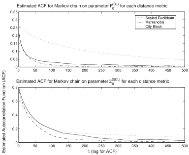
Figure 1: Estimated Autocorrelation Function (ACF) for parameters $F_{0}$ and $\Xi^{2}_{0}$.

Autocorrelation Function: Figure 1 shows the estimated autocorrelation functions for the Markov chains of the random variables $F_{0}$ and $\Xi_{0}^{2}$. We analyze the marginal parameters to get a reasonable estimate of the mixing behavior of the MCMC-ABC algorithm. The results demonstrate the degree of serial correlation in the Markov chains generated for these parameters as a function of lag time $\tau$. The higher the decay rate in the tail of the estimated ACF as a function of $\tau$, the better the mixing of the MCMC algorithm. Due to the independence properties of this model there is little difference between results obtained for Scaled Euclidean and Mahlanobis distances. As shown in Appendix C, the estimate of the covariance matrix is diagonal on all but the right lower $2\times 2$ block. Hence, we recommend using the simple Scaled Euclidean distance metric as it provided the best trade-off between simplicity and mixing performance.

Geweke Time Series Diagnostic: Figure 2 shows results for the Geweke time series diagnostic. Again, we present the results for the random variables $F_{0}$ and $\Xi_{0}^{2}$. Note, we used the posterior mean as the sample function and a set of increasing values for $\widetilde{T}$ from $T_{b}+5,000$ increasing in steps of 5,000 samples to $T$. In each case we split the chain in each “window” given by $\{\theta_{i}^{(t)}\}_{t=1:T_{1}}$ and $\{\theta_{i}^{(t)}\}_{t=T^{*}:\widetilde{T}}$ according to recommendations from Geweke et al. [10]. We then calculate the convergence diagnostic $Z_{\widetilde{T}}$ which is the difference between these two means divided by the asymptotic standard error of their difference. As the chain length increases $\widetilde{T}\rightarrow\infty$, the sampling distribution of $Z\rightarrow{\cal N}(0,1)$ if the chain has converged. Hence values of $Z_{\widetilde{T}}$ in the tails of a standard normal distribution suggest that the chain was not fully converged early on (i.e. during the 1st window). Hence, we plot $Z_{\widetilde{T}}$ scores versus increasing $\widetilde{T}$ and monitor if they lie within a $95\%$ confidence interval $Z_{\widetilde{T}}\in[-1.96,1.96]$. The results in Figure 2 clearly demonstrate the convergence properties of the distance functions differ. Again this is more material in the Markov chain for the variance parameter when compared to the Markov chain results for the chain ladder factor. The main point we note is that again one would advise against use of the “City block” distance metric.

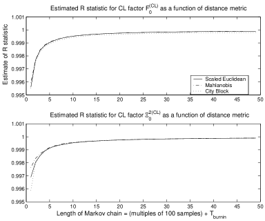
Figure 3: Estimated R statistic for parameters $F_{0}$ and $\Xi^{2}_{0}$ as a function of the length of the Markov chain $\widetilde{T}$.

Gelman and Rubin R statistic: Figure 3 presents the Gelman and Rubin convergence diagnostic. To calculate this we ran 20 chains in parallel, each of length 10,000 samples and for each chain we discarded 250 samples as burn-in. We then estimated the $R$ statistic as a function of simulation time post burn-in. Figure 3 shows the convergence rate of the $R$ statistic to 1 for each distance metric on increasing blocks of 200 samples. Using this summary statistic, all three distance metrics are very similar in terms of convergence rate of the R statistic to 1.

Overall, these three convergence diagnostics demonstrate that the simple scaled Euclidean distance metric is the superior choice. Secondly, we see appropriate convergence of the Markov chains under three convergence diagnostics which tests different aspects of the mixing of the Markov chains, giving confidence in the performance of the MCMC-ABC algorithm for this model.

6.4 Bayesian parameter estimates

In this section we present results for the scaled Euclidean distance metric, with a Markov chain of length 200,000 samples discarding the first 50,000 samples as burn-in. Table 4 shows the CL parameter estimates for the DFCL model and the associated parameter estimation error. We define the following quantities:

• $\widehat{f}^{(MAP)}_{j}|\sigma_{0:J-1}$, $\widehat{f}^{(MMSE)}_{j}|\sigma_{0:J-1}$, $\widehat{\sigma}_{f_{j}}|\sigma_{0:J-1}$ and $[\hat{q}_{0.05},\hat{q}_{0.95}]|\sigma_{0:J-1}$ denote respectively the Maximum a-Posteriori, Minimum Mean Square Error, posterior standard deviation of the conditional distribution of chain ladder factor $F_{j}$ and the posterior coverage probability estimates at $5\%$ of the conditional distribution of chain ladder factor $F_{j}$. Each of these estimates is conditional on knowledge of the true $\sigma_{0:J-1}$.

• $\widehat{f}^{(MAP)}_{j}$, $\widehat{f}^{(MMSE)}_{j}$, $\widehat{\sigma}_{f_{j}}$ and $[\hat{q}_{0.05},\hat{q}_{0.95}]$ denote the same quantities for the unconditional distribution after joint estimation of $F_{0:J-1}$ and $\Xi_{0:J-1}$.

• $Ave[A\left(\theta_{1:2J},f_{j}\right)]$ and $Ave[A\left(\theta_{1:2J},\sigma_{j}\right)]$ denote the average acceptance probabilities of the Markov chain.

• $\widehat{\sigma}^{2(MAP)}_{j}$, $\widehat{\sigma}^{2(MMSE)}_{j}$, $\widehat{\sigma}_{\sigma^{2}_{j}}$ and $[\hat{q}_{0.05},\hat{q}_{0.95}]$ denote the same quantities for the chain ladder variances as those defined above for chain ladder factors.

Note, the estimates for $\widehat{f}^{(MAP)}_{j}$ and $\widehat{\sigma}^{(MAP)}_{j}$ were obtained marginally. For the frequentist approach we obtain the standard error in the estimates by using 1,000 bootstrap realisations of $\left\{\mathcal{D}_{I}^{\left(s\right)}\right\}_{s=1:1,000}$ to obtain $\left\{\widetilde{\bm{f}}_{\left(s\right)}^{\left(CCL\right)},\widetilde{\bm{\sigma}}_{\left(s\right)}^{2\left(CCL\right)}\right\}_{s=1:1,000}$. We use these bootstrap samples to calculate the standard deviation in the estimates of the parameters in the classical frequentist CL approach, given in brackets $\left(.\right)$ next to their corresponding estimators. The standard errors in the Bayesian parameter estimates are obtained by blocking the Markov chain into 100 blocks of length 1,500 samples and estimating the posterior quantities on each block.

7 Example 2: Real Claims Reserving data

In this example we consider estimation using real claims reserving data from Wüthrich-Merz [30], see Table 3. This yearly loss data is turned into annual cumulative claims and divided by 10,000 for the analysis in this example. We use the analysis from the previous study to justify use of the joint MCMC-ABC simulation algorithm with a scaled Euclidean distance metric.

We pre-tuned the coefficient of variation of the Gamma proposal distribution for each parameter of the posterior. This was performed using the following settings: $T_{b}=50,000$, $\widetilde{T}=200,000$, $\epsilon^{\min}=10^{-5}$ and initial values $\gamma_{j}=1$ for all $j\in\{1,\ldots,2J\}$. Here we make a strict requirement of the tolerance level to ensure we have accurate results from our ABC approximation. Additionally, the prior parameters for the chain ladder factors $F_{j}$ were set as $\left(\alpha_{j},\beta_{j}\right)=\left(1,\widehat{f}^{(CL)}_{j}\right)$ and the parameters for the variance $\Xi^{-2}_{j}$ priors were set as $\left(a_{j},b_{j}\right)=\left(1,\widehat{\sigma}^{(CL)}_{j}\right)$. The code for this problem was written in Matlab and it took approximately 10 min to simulate 200,000 samples from the MCMC-ABC algorithm on Intel Xeon 3.4GHz processor with 2Gb RAM.

After tuning the proposal distributions during burn-in we obtained rounded shape parameters
$\gamma_{1:9}=[50;100;500;500;5,000;20,000;100,000;2,000,000;3,000,000]$ provided average acceptance probabilities between 0.3 and 0.5.

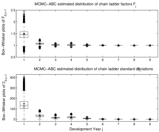
Figure 4: Box-Whisker plots of parameters $\bm{F}$ and $\bm{\Xi}$ with each box marking the $25^{th},50^{th},75^{th}$ percentiles. Top: 200,000 MCMC-ABC samples to estimate posterior for $\bm{F}$. The sample mean and mode are denoted by ’*’ and ’o’ respectively. The classical estimators $\widehat{\bm{f}}^{(CL)}$ are denoted by $\triangle$. Bottom: 200,000 MCMC-ABC samples to estimate posterior for $\bm{\Xi}$. The sample mean and mode are denoted by ’*’ and ’o’ respectively. The classical estimators $\widehat{\bm{\sigma}}^{(CL)}$ are denoted by ’$\triangle$’.

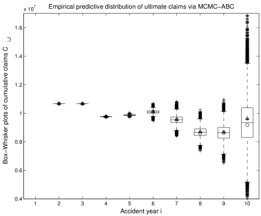
Figure 5: Box-Whisker plots of predictive distribution of cumulative ultimate claims $C_{1:J}$ with the box marking the $25^{th},50^{th},75^{th}$ percentiles; see also Table 6. The mean predicted ultimate claims under a Bayesian approach (using MMSE point estimates) are marked with ’*’, the predicted mode for the ultimate claims (using MAP point estimates) is marked with ’o’ and the mean predicted ultimate claims under the DFCL classical method are marked with ’$\triangle$’.

Estimates of $\bm{f}$ and $\bm{\sigma}$
Figures 4 presents box-whisker plots of estimates of the distributions of the parameters $F_{0:J-1}$ and $\Xi_{0:J-1}$ obtained from the MCMC-ABC algorithm, post burn-in. Figure 5 shows the Bayesian MCMC-ABC empirical distributions of the ultimate claims, $C_{i,J}$ for $i=1,\ldots,I$. In Table 5 we present the predicted cumulative claims for each year along with the estimates for the chain ladder factors and chain ladder variances under both the classical approach and the Bayesian model. We see that with this fairly vague prior specified, we do indeed obtain convergence of the MCMC-ABC based Bayesian estimates $\widehat{\bm{f}}^{(MMSE)},\widehat{\bm{\sigma}}^{(MMSE)}$ to the classical estimates $\widehat{\bm{f}}^{(CL)},\widehat{\bm{\sigma}}^{(CL)}$.

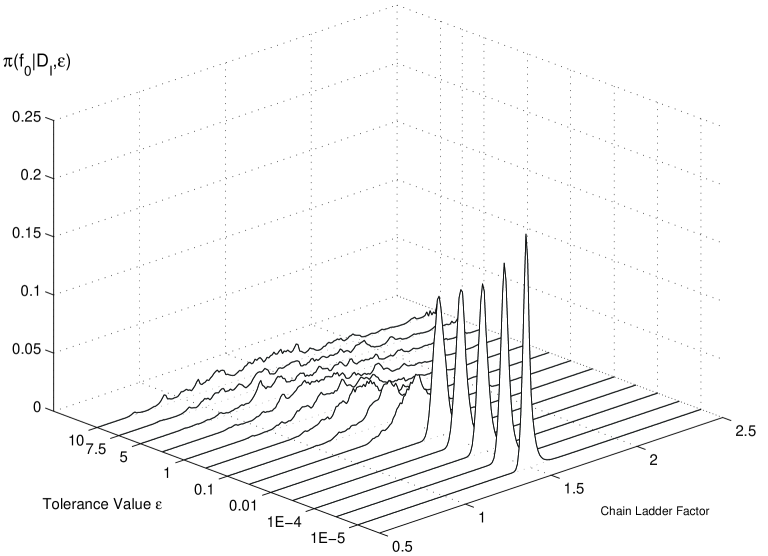
Figure 6: Distribution of the chain ladder factor $F_{0}$ as a function of tolerance.

Dependence on tolerance $\epsilon$
Figure 6 presents a study of the histogram estimate of the marginal posterior distribution for chain ladder factor $\pi_{ABC}\left(f_{0}|\mathcal{D}_{I},\epsilon^{\min}\right)$. The plot was obtained by sampling from the full posterior $\pi_{ABC}\left(\bm{f},\bm{\sigma}|\mathcal{D}_{I},\epsilon^{\min}\right)$ for each specified tolerance value, $\epsilon^{\min}$. Then the samples for the particular chain ladder parameter in each plot are turned into a smoothed histogram estimate for each $\epsilon^{\min}$ and plotted. The results of this analysis demonstrated that when $\epsilon$ is large, in this model greater than around $\epsilon^{\min}=0.1$, the likelihood is not having an influence on the ABC posterior distribution. Hence, under an MCMC-ABC algorithm, this results in acceptance probabilities for the chain being artificially high, resulting in estimates of the posterior which reflect the prior distribution used (in this case a vague prior). As $\epsilon^{\min}$ is reduced, we notice that the changes in the estimate of the posterior distribution also reduces. The aim of this study is to demonstrate that once $\epsilon^{\min}$ reaches a small enough level, the effect of reducing it further is minimal on the posterior distribution. We see that changing $\epsilon^{\min}$ from $10^{-4}$ to $10^{-5}$ has not had a material impact on the posterior mean or variance, the change is less than $10\%$. As a result, reducing $\epsilon^{\min}$ past this point cannot be justified relative to the significant increase in computational effort required to achieve such a further reduction in $\epsilon^{\min}$.

Ultimately, we would like an algorithm which could work well for any $\epsilon^{\min}$, the smaller the better. However, we note that with a decreasing $\epsilon^{\min}$ in the sampler we present in this paper, one must take additional care to ensure the Markov chain is still mixing and not “stuck” in a particular state, as is observed to be the case in all MCMC-ABC algorithms. To avoid this acknowledged difficulty with MCMC-ABC, one should run much longer MCMC chains or alternatively use of more sophisticated sampling algorithms such as SMC Samplers PRC-ABC based algorithms; see Sisson et al.  [25].

The conclusion of these findings is that a value of $\epsilon^{\min}=10^{-5}$, which was used for the analysis of the data in this paper, is suitable numerically and computationally.




VaR and MSEP.
In Table 6 we present the predictive VaR at $95\%$ and $99\%$ levels for the ultimate predicted claims, obtained from the MCMC-ABC algorithm. These are easily obtained under the Bayesian setting, using the MCMC-ABC posterior samples to explicitly obtain samples from the full predictive distribution of the cumulative claims after integrating out the parameter uncertainty numerically. In addition to this, we present the analysis of the MSEP under the bootstrap frequentist procedure and the Bayesian MCMC-ABC and credibility estimates for the total predicted cumulative claims for each accident year $i$. We also present results for the sum of the total cumulative claims for each accident year, and the associated parameter uncertainty and process variance (see Section 4 for details).

We can make the following conclusions from these results:

1. The estimates of process variance for each $C_{i,J}$ demonstrate that the frequentist bootstrap and the credibility estimates are very close for all accident years $i$. The Bayesian results compare favorably with the credibility results.

2. The results for the parameter estimation error for the predicted cumulative claims $C_{i,J}$ demonstrate for small $i$ that the Bayesian approach results in a smaller estimation error compared to the frequentist approach. For large $i$, the Bayesian approach produces larger estimation error relative to the credibility approach.

3. The total results for the process variance for $C=\sum_{i}C_{i,J}$ demonstrate that the frequentist and credibility results are very close. Additionally, Bayesian total results are largest followed by credibility and then frequentist estimates which is in agreement with theoretical bounds.

4. The total results for the parameter estimation error for $C=\sum_{i}C_{i,J}$ demonstrate that frequentist unconditional bootstrap procedure results in the lowest total error. The Bayesian approach and credibility total parameter errors are close. Additionally, we note that the results in Table 7.1 of Wüthrich-Merz [30], for the total parameter estimation error under an unconditional frequentist bootstrap with unscaled residuals is also very close to the total obtained under the frequentist approach.

8 Discussion

This paper has presented a distribution-free claims reserving model under a Bayesian paradigm. A novel advanced MCMC-ABC algorithm was developed to obtain estimates from the resulting intractable posterior distribution of the chain ladder factors and chain ladder variances. We assessed several aspects of this algorithm, including the properties of the convergence of the MCMC algorithm as a function of the distance metric approximation in the ABC component. The methodologies performance was demonstrated on a synthetic data set generated from known parameters. Next, it was applied to a real claims reserving data set. The results we obtained for predicted cumulative ultimate claims were compared to those obtained via classical chain ladder methods and via credibility theory. This clearly demonstrated that the algorithm is working accurately and provides us not only with the ability to obtain point estimates for the first and second moments of the ultimate cumulative claims, but also with an accurate empirical approximation of the entire distribution of the ultimate claims. This is valuable for many reasons, including prediction of reserves which are not based on centrality measures such as the tail based VaR results we present.

Acknowledgements
The fist author thanks ETH FIM and ETH Risk Lab for their generous financial assistance whilst completing aspects of this work at ETH. The first author also thanks the Department of Mathematics and Statistics at the University of NSW for support through an Australian Postgraduate Award and to CSIRO for support through a postgraduate research top up scholarship. Finally, this material was based upon work partially supported by the National Science Foundation under Grant DMS-0635449 to the Statistical and Applied Mathematical Sciences Institute, North Carolina, USA. Any opinions, findings, and conclusions or recommendations expressed in this material are those of the author(s) and do not necessarily reflect the views of the National Science Foundation

Appendix A ABC algorithm

The ABC algorithm is typically justified in the simple rejection sampling framework. This then extends in a straightforward manner to other sampling frameworks such as the MCMC algorithm we utilise in this paper. We denote the posterior density from which we wish to draw samples by $\pi\left(\theta|y\right)\propto\pi\left(y|\theta\right)\pi\left(\theta\right)$ with $\theta\in\Omega$, where $\Omega$ denotes support of the posterior distribution and ${\cal Y}$ is the support for $y$.

The ABC method aims to draw from this posterior density $\pi\left(\theta|y\right)$ without the requirement of evaluating the computationally expensive or in our setting intractable likelihood $\pi\left(y|\theta\right)$. The cost of avoiding this calculation is that we obtain an “approximation”.

1st case. We assume that the support ${\cal Y}$ is discrete. Given an observation $y\in{\cal Y}$, we would like to sample from $\pi\left(\theta|y\right)$. Then the original rejection sampling algorithm reads as follows:

Rejection Sampling ABC

1. Sample $\theta^{\prime}$ from prior $\pi\left(\theta\right)$;

2. Simulate synthetic data set of auxiliary variables $x|\theta^{\prime}\sim\pi\left(x|\theta^{\prime}\right)$;

3. ABC Rejection condition: if $x=y$ then accept sample $\theta^{\prime}$, else reject sample and return to step 1.

Then the chosen $\theta^{\prime}$ is distributed from $\pi(\theta|y)$. This follows from a simple rejection argument, Denote $\{x=y\}$ if $\theta^{\prime}$ was chosen. Then, the joint density of $(\theta^{\prime},x)$ conditional on $\{y,x=y\}$ is given by

$$\pi(\theta,x|y,x=y)=\frac{\pi(\theta)\pi(x|\theta)\mathbb{I}\{y\}(x)}{\int\pi(\theta)\pi(y|\theta)d\theta}=\left\{\begin{array}[]{ll}\frac{\pi(\theta,y)}{\pi(y)}=\pi(\theta|y)&\text{ if }x=y,\\ 0&\text{ otherwise.}\end{array}\right.$$ (A.1)

This implies that

$$\sum_{x\in{\cal Y}}\pi(\theta,x|y,x=y)=\pi(\theta|y).$$ (A.2)

Henceforth, this algorithm generates samples $\theta^{(t)}\sim\pi(\theta|y)$, for $t=1,\ldots,T$.

2nd case. For more general supports ${\cal Y}$ one replaces the strict equality $x=y$ with a tolerance $\epsilon>0$ and a measure of discrepancy or a distance metric $\rho(x,y)\leq\epsilon$. In this case the posterior distribution is given by $\pi(\theta,x|y,\rho(x,y)<\epsilon)$. Implementing this algorithm in a rejection sampling framework gives the following:

Rejection Sampling ABC

1. Sample $\theta^{\prime}$ from prior $\pi\left(\theta\right)$;

2. Simulate synthetic data set of auxiliary variables $x|\theta^{\prime}\sim\pi\left(x|\theta^{\prime}\right)$;

3. ABC Rejection Condition 2: If $\rho(x,y)<\epsilon$ then accept sample $\theta^{\prime}$, else reject sample and return to step 1.

In this case the joint density of $(\theta^{\prime},x)$, conditional on $\{y,\rho(x,y)<\epsilon\}$, is given by

$$\pi(\theta,x|y,\rho(x,y)<\epsilon)=\frac{\pi(\theta)~{}\pi(x|\theta)~{}\mathbb{I}\{\rho(x,y)<\epsilon\}(x)}{\int\pi(\theta)~{}\pi(x|\theta)~{}\mathbb{I}\{\rho(x,y)<\epsilon\}(x)~{}dxd\theta}.$$ (A.3)

Note that for appropriate choices of the distance metric $\rho$ and assuming the necessary continuity properties for the densities we obtain that

$$\lim_{\epsilon\to 0}\int_{\cal Y}\pi(\theta,x|y,\rho(x,y)<\epsilon)dx=\pi(\theta|y).$$ (A.4)

This concept was taken further with the intention of improving the simulation efficiency by reducing the number of rejected samples. To achieve this, sufficient statistics were used to replace the comparison between the auxiliary variables (“synthetic data”) $x$ and the observations $y$. Denoting the sufficient statistics by $S(y)$ and $S(x)$, allows one to decompose the likelihood under the Fisher-Neyman factorization theorem into $\pi(y|\theta)=f(y)g(S(y)|\theta)$ for appropriate functions $f$ and $g$. In the ABC context presented above, the consequence of this decomposition is that when $\rho(S(y),S(x))<\epsilon$ the obtained samples are from the posterior density $\pi(\theta,x|y,\rho(S(y),S(x))<\epsilon)$ similar to (A.3). In general, summary statistics will be used when sufficient statistics are not attainable.

Appendix B MCMC-ABC to sample from $\pi_{ABC}\left(\bm{f},\bm{\sigma}|\mathcal{D}_{I}\right)$

We develop an MCMC-ABC algorithm which has an adaptive proposal mechanism and annealing of the tolerance during burn-in of the Markov chain. Having reached the final tolerance post annealing, denoted $\epsilon^{\min}$, we utilise the remaining burn-in samples to tune the proposal distribution to ensure an acceptance probability between the range of 0.3 and 0.5 is achieved. The optimal acceptance probability when posterior parameters are i.i.d. Gaussian was proven to be at 0.234; see Roberts et al. [20]. Though our problem does not match the required conditions for this proof, it provides a practical guide. To achieve this, we tune the coefficient of variation of the proposal, in our case it is the shape parameter of the Gamma proposal distribution. We impose an additional constraint that the minimum shape parameter value is set at $\gamma_{j}^{\min}$ for $j\in\{1,\ldots,2J\}$.

MCMC-ABC algorithm using bootstrap samples.

1. For $t=0$ initialize the parameter vector randomly, this gives $\theta_{1:2J}^{\left(0\right)}=\left(f_{0:J-1}^{\left(0\right)},\sigma_{0:J-1}^{\left(0\right)}\right)$. Initialize the proposal shape parameters $\gamma_{j}\geq\gamma_{j}^{\min}$ for all $j\in\{1,\ldots,2J\}$.

2. For $t=1,\ldots,T$

   1. Set $\left(\theta_{1:2J}^{\left(t\right)}\right)=\left(\theta_{1:2J}^{\left(t-1\right)}\right)$.

   2. For $j=1,\ldots,2J$

      1. Sample proposal $\theta_{j}^{\ast}$ from a $\Gamma(\gamma_{j},\theta_{j}^{(t)}/\gamma_{j})$-distribution. We denote the Gamma proposal density by $K\left(\theta_{j}^{\ast};\gamma_{j},{\theta_{j}^{(t)}}/{\gamma_{j}}\right)$. This gives proposed parameter vector $\bm{\theta}^{\ast}=\left(\theta_{1:j-1}^{(t)},\theta_{j}^{\ast},\theta_{j+1:2J}^{(t)}\right)$.

      2. Conditional on $\bm{\theta}^{\ast}=\left(\theta_{1:j-1}^{(t)},\theta_{j}^{\ast},\theta_{j+1:2J}^{(t)}\right)$, generate synthetic bootstrap data set $\mathcal{D}_{I}^{\ast}=\mathcal{D}_{I}^{\ast}\left(\bm{\theta}^{\ast}\right)$ using the bootstrap procedure detailed in Section 4 where we replace the CL parameter estimates $(\widehat{\bm{f}}^{(CL)},\widehat{\bm{\sigma}}^{(CL)})$ by the parameters $\bm{\theta}^{\ast}$.

      3. Evaluate summary statistics $S\left(\mathcal{D}_{I};0,1\right)$ and $S\left(\mathcal{D}_{I}^{\ast};{\mu}^{\ast};{s}^{\ast}\right)$ and corresponding decision function $g({\cal D}_{I}|{\cal D}_{I}^{\ast})$ as described in Section 5.

      4. Accept proposal with ABC acceptance probability

         $$A\left(\theta_{1:2J}^{\left(t\right)},\bm{\theta}^{\ast}\right)=\min\left\{1,\frac{\pi\left(\theta_{j}^{\ast}\right)K\left(\theta_{j}^{(t)};\gamma_{j},{\theta_{j}^{\ast}}/{\gamma_{j}}\right)}{\pi\left(\theta_{j}^{\left(t\right)}\right)K\left(\theta_{j}^{\ast};\gamma_{j},{\theta_{j}^{(t)}}/{\gamma_{j}}\right)}~{}g({\cal D}_{I}|{\cal D}_{I}^{\ast})\right\}.$$

         That is, simulate $U\sim{\cal U}(0,1)$ and set $\theta_{j}^{\left(t\right)}=\theta_{j}^{\ast}$ if $U<A\left(\theta_{1:2J}^{\left(t\right)},\bm{\theta}^{\ast}\right)$.

      5. If $100\leq t\leq T_{b}$ and $\epsilon_{t}=\epsilon^{\text{min}}$ then check to see if tuning of the proposal is required. Define the average acceptance probability over the last 100 iterations of updates for parameter $i$ by $\bar{a}_{i}^{(t-100:t)}$ and consider the adaption:

         $$\gamma_{j}^{*}=\left\{\begin{array}[]{l l l}0.9\gamma_{j}&\quad\mbox{ if $\bar{a}_{i}^{(t-100:t)}<0.3$ and $\gamma_{j}>\gamma_{j}^{\text{min}}$},\\ 1.1\gamma_{j}&\quad\mbox{ if $\bar{a}_{i}^{(t-100:t)}>0.5$},\\ \gamma_{j}&\quad\mbox{ otherwise.}\\ \end{array}\right.$$

         Then set the proposal shape parameter as $\gamma_{j}=\text{max}\{\gamma_{j}^{*},\gamma_{j}^{\text{min}}\}$.

The MCMC-ABC algorithm presented can be enhanced by utilising an idea of Gramacy et al. [13] in an ABC setting. This involves a combination of tempering the tolerance $\{\epsilon_{t}\}_{t=1:T}$ and importance sampling corrections.

B.1 ABC algorithmic choices for the time series DFCL model

We start with the choices of the ABC components.

• Generation of a synthetic data set: Note that in this setting not only is the likelihood intractable but also the generation of a synthetic data set $\mathcal{D}_{I}^{\ast}$ given the current parameter values $\bm{F},\bm{\Xi}$ is not straightforward. The synthetic data set $\mathcal{D}_{I}^{\ast}$ is generated using the bootstrap procedure described in Section 4. Note that both the bootstrap residual $\widetilde{\varepsilon}_{i,j}$ and the bootstrap samples $\mathcal{D}_{I}^{\ast}$ are functions of the parameter choices; see Section 4.1. Therefore we generate for given $\bm{F}=\bm{f}$ and $\bm{\Xi}=\bm{\sigma}$ the bootstrap residuals $\widetilde{\varepsilon}_{i,j}=\widetilde{\varepsilon}_{i,j}(f_{j-1},\sigma_{j-1})$ and the bootstrap samples $\mathcal{D}_{I}^{\ast}=\mathcal{D}_{I}^{\ast}(\bm{f},\bm{\sigma})$ according to the non-parametric bootstrap (see Section 4.1) where we replace the CL parameter estimates $(\widehat{\bm{f}}^{(CL)},\widehat{\bm{\sigma}}^{(CL)})$ by the parameters $\theta=(\bm{F},\bm{\Xi})$.

• Summary statistics: We introduce summary statistics to replace sufficient statistics when they are not attainable for a given model. Then, in order to define the decision function $g$, we introduce summary statistics; see Appendix A. For the observed data $\mathcal{D}_{I}$ we define the vector

  $$S\left(\mathcal{D}_{I};0,1\right) = \left(S_{1},\ldots,S_{n+2}\right)$$

  $$= \left(C_{0,1},\ldots,C_{0,J},C_{1,1},\ldots,C_{0,J-1},\ldots,C_{I-2,1},C_{I-2,2},C_{I-1,1};0,1\right),$$

  where $n$ denotes the number of residuals $\widetilde{\varepsilon}_{i,j}$. For given $\theta=(\bm{F},\bm{\Xi})$, we generate the bootstrap sample $\mathcal{D}_{I}^{\ast}=\mathcal{D}_{I}^{\ast}(\bm{F},\bm{\Xi})$ as described above. The corresponding residuals $\widetilde{\varepsilon}_{i,j}=\widetilde{\varepsilon}_{i,j}(F_{j-1},\Xi_{j-1})$ should also be close to the standardized observations. Therefore, we define its empirical mean and standard deviation by

  $$\mu^{\ast} = \mu^{\ast}(\bm{F},\bm{\Xi})~{}=~{}\frac{1}{n}\sum_{i,j}\widetilde{\varepsilon}_{i,j}(F_{j-1},\Xi_{j-1}),$$ (B.2)

  $$s^{\ast} = s^{\ast}(\bm{F},\bm{\Xi})~{}=~{}\left[\frac{1}{n-1}\sum_{i,j}\left(\widetilde{\varepsilon}_{i,j}(F_{j-1},\Xi_{j-1})-\mu^{\ast}(\bm{F},\bm{\Xi})\right)^{2}\right]^{1/2}.$$ (B.3)

  Hence, the summary statistics for the synthetic data is given by

  $$S\left(\mathcal{D}^{\ast}_{I};\mu^{\ast},s^{\ast}\right)=\left(C^{\ast}_{0,1},\ldots,C^{\ast}_{0,J},C^{\ast}_{1,1},\ldots,C^{\ast}_{0,J-1},\ldots,C^{\ast}_{I-2,1},C^{\ast}_{I-2,2},C^{\ast}_{I-1,1};\mu^{\ast},s^{\ast}\right).$$

• Distance metrics:

  • Mahlanobis distance and scaled Euclidean distance

    Here we draw on the analysis of Sisson et al. [8] that proposes the use of the Mahlanobis distance metric given by

    $$\rho\left(S\left(\mathcal{D}_{I};0,1\right),S\left(\mathcal{D}_{I}^{\ast};\mu^{\ast},s^{\ast}\right)\right)$$

    $$= \left[S\left(\mathcal{D}_{I};0,1\right)-S\left(\mathcal{D}_{I}^{\ast};\mu^{\ast},s^{\ast}\right)\right]^{\top}~{}\Sigma_{\mathcal{D}_{I}}^{-1}~{}\left[S\left(\mathcal{D}_{I};0,1\right)-S\left(\mathcal{D}_{I}^{\ast};\mu^{\ast},s^{\ast}\right)\right],$$

    where the covariance matrix $\Sigma_{\mathcal{D}_{I}}$ is an appropriate scaling described in Appendix C. The scaled Euclidean distance is obtained when we only consider the diagonal elements of the covariance matrix $\Sigma_{\mathcal{D}_{I}}$.

    Note, the covariance matrix $\Sigma_{\mathcal{D}_{I}}$ provides a weighting on each element of the vector of summary statistics to ensure they are scaled appropriately according to their influence on the ABC approximation. There are many other such weighting schemes one could conceive.

  • Manhattan “City Block” distance

    We consider the $L^{1}$-distance given by

    $$\rho\left(S\left(\mathcal{D}_{I};0,1\right),S\left(\mathcal{D}_{I}^{\ast};\mu^{\ast},s^{\ast}\right)\right)=\sum_{i=1}^{n+2}\left|S_{i}\left(\mathcal{D}_{I};0,1\right)-S_{i}\left(\mathcal{D}_{I}^{\ast};\mu^{\ast},s^{\ast}\right)\right|.$$

• Decision function: We work with a hard decision function given by

  $$g\left(\mathcal{D}_{I}|\mathcal{D}_{I}^{\ast}\right)=\mathbb{I}\left\{\rho\left(S\left(\mathcal{D}_{I};0,1\right),S\left(\mathcal{D}_{I}^{\ast};\mu^{\ast},s^{\ast}\right)\right)<\epsilon\right\}.$$

• Tolerance schedule: We use the sequence

  $$\epsilon_{t}=\max\left\{20,000-10t,\epsilon^{\min}\right\}.$$

  Note, the use of an MCMC-ABC algorithm can result in “sticking” of the chain for extended periods. Therefore, one should carefully monitor convergence diagnostics of the resulting Markov chain for a given tolerance schedule. There is a trade-off between the length of the Markov chain required for samples approximately from the stationary distribution and the bias introduced by non zero tolerance. In this paper we set $\epsilon^{\min}$ via preliminary analysis of the Markov chain sampler mixing rates for a transition kernel with coefficient of variation set to one.

  We note that in general, practitioners will have a required precision in posterior estimates that can be directly used to determine, for a given computational budget, a suitable tolerance $\epsilon^{\min}$.

• Convergence diagnostics: We stress that when using an MCMC-ABC algorithm, it is crucial to carefully monitor the convergence diagnostics of the Markov chain. This is more important in the ABC context than in the general MCMC context due to the possibility of extended rejections where the Markov chain can stick in a given state for long periods. This can be combatted in several ways which will be discussed once the algorithm is presented.

  The convergence diagnostics we consider are evaluated only on samples post annealing of the tolerance threshold and after an initial burn-in period once tolerance of $\epsilon^{\min}$ is reached. If the total chain has length $T$, the initial burn-in stage will correspond to the first $T_{b}$ samples and we define $\widetilde{T}=T-T_{b}$. We denote by $\{\theta_{i}^{(t)}\}_{t=1:\widetilde{T}}$ the Markov chain of the $i$-th parameter after burn-in. The diagnostics we consider are given by:

  • Autocorrelation. This convergence diagnostic will monitor serial correlation in the Markov chain. For given Markov chain samples for the $i$-th parameter $\{\theta_{i}^{(t)}\}_{t=1:\widetilde{T}}$, we define the biased autocorrelation estimate at lag $\tau$ by

    $$\widehat{ACF}(\theta_{i},\tau)=\frac{1}{(\widetilde{T}-\tau)\hat{\sigma}\left(\theta_{i}\right)}\sum_{t=1}^{\widetilde{T}-\tau}[\theta_{i}^{(t)}-\widehat{\mu}\left(\theta_{i}\right)][\theta_{i}^{(t+\tau)}-\widehat{\mu}\left(\theta_{i}\right)],$$ (B.4)

    where $\widehat{\mu}\left(\theta_{i}\right)$ and $\hat{\sigma}\left(\theta_{i}\right)$ are the estimated mean and standard deviation of $\theta_{i}$.

  • Geweke [10] time series diagnostic. For parameter $\theta_{i}$ it is calculated as follows:

    1. Split the Markov chain samples into two sequences, $\{\theta_{i}^{(t)}\}_{t=1:T_{1}}$ and $\{\theta_{i}^{(t)}\}_{t=T^{*}:\widetilde{T}}$, such that $T^{*}=\widetilde{T}-T_{2}+1$, and with ratios $T_{1}/\widetilde{T}$ and $T_{2}/\widetilde{T}$ fixed such that $(T_{1}+T_{2})/\widetilde{T}<1$ for all $\widetilde{T}$.

    2. Evaluate $\widehat{\mu}\left(\theta_{i}^{T_{1}}\right)$ and $\widehat{\mu}\left(\theta_{i}^{T_{2}}\right)$ corresponding to the sample means on each sub sequence.

    3. Evaluate consistent spectral density estimates for each sub sequence, at frequency 0, denoted $\widehat{SD}(0;T_{1},\theta_{i})$ and $\widehat{SD}(0;T_{2},\theta_{i})$. The spectral density estimator considered in this paper is the classical non-parametric periodogram or power spectral density estimator. We use Welch’s method with a Hanning window; for details see Appendix D.

    4. Evaluate convergence diagnostic given by
       $Z_{\widetilde{T}}=\frac{\widehat{\mu}\left(\theta_{i}^{T_{1}}\right)-\widehat{\mu}\left(\theta_{i}^{T_{2}}\right)}{T_{1}^{-1}\widehat{SD}(0;T_{1},\theta_{i})+T_{2}^{-1}\widehat{SD}(0;T_{2},\theta_{i})}.$
       According to the central limit theorem, as $\widetilde{T}\rightarrow\infty$ one has that $Z_{\widetilde{T}}\rightarrow{\cal N}(0,1)$ if the sequence $\{\theta_{i}^{(t)}\}_{t=1:\widetilde{T}}$ is stationary.

  • Gelman-Rubin [9] R-statistic diagnostic. This approach to convergence analysis requires that one runs multiple parallel independent Markov chains each starting at randomly selected initial starting points (we run five chains). For comparison purposes we split the total computational budget of $\widetilde{T}$ into $T_{1}=T_{2}=\ldots=T_{5}=\frac{\widetilde{T}}{5}$. The convergence diagnostic for parameter $\theta_{i}$ is calculated using the following steps:

    1. Generate five independent Markov chain sequences, producing the chains for parameter $\theta_{i}$ denoted $\{\theta_{i,k}^{(t)}\}_{t=1:T_{k}}$ for $k\in\{1,\ldots,5\}$.

    2. Calculate the sample means $\widehat{\mu}\left(\theta_{i}^{T_{k}}\right)$ for each sequence and the overall mean $\widehat{\mu}\left(\theta_{i}^{\widetilde{T}}\right)$.

    3. Calculate the variance of the sequence means
       $\frac{1}{4}\sum_{k=1}^{5}\left(\widehat{\mu}\left(\theta_{i}^{T_{k}}\right)-\widehat{\mu}\left(\theta_{i}^{\widetilde{T}}\right)\right)^{2}\stackrel{{\scriptstyle def.}}{{=}}B_{i}/T_{k}.$

    4. Calculate the within-sequence variances $\widehat{s}^{2}\left(\theta_{i}^{T_{k}}\right)$ for each sequence.

    5. Calculate the average within-sequence variance, $\frac{1}{5}\sum_{k=1}^{5}\widehat{s}^{2}\left(\theta_{i}^{T_{k}}\right)\stackrel{{\scriptstyle def.}}{{=}}W_{i}$.

    6. Estimate the target posterior variance for parameter $\theta_{i}$ by the weighted linear combination $\widehat{\sigma}^{2}\left(\theta_{i}^{\widetilde{T}}\right)=\frac{T_{k}-1}{T_{k}}W_{i}+\frac{1}{T_{k}}B_{i}$. This estimate is unbiased for samples which are from the stationary distribution. In the case in which not all sub chains have reached stationarity, this overestimates the posterior variance for a finite $\widetilde{T}$ but asymptotically, $\widetilde{T}\rightarrow\infty$, it converges to the posterior variance.

    7. Improve on the Gaussian estimate of the target posterior given by
       $\mathcal{N}(\widehat{\mu}\left(\theta_{i}^{\widetilde{T}}\right),\widehat{\sigma}^{2}\left(\theta_{i}^{\widetilde{T}}\right))$ by accounting for sampling variability in the estimates of the posterior mean and variance. This can be achieved by making a Student-t approximation with location $\widehat{\mu}\left(\theta_{i}^{\widetilde{T}}\right)$, scale $\sqrt{\widehat{V}_{i}}$ and degrees of freedom $df_{i}$, each given respectively by:
       $\widehat{V}_{i}=\widehat{\sigma}^{2}\left(\theta_{i}^{\widetilde{T}}\right)+\frac{B_{i}}{\widetilde{T}}$ and $df_{i}=\frac{2\widehat{V}_{i}^{2}}{\widehat{\text{Var}}(\widehat{V}_{i})}$, where the variance is estimated as
       

       $$\begin{split}\widehat{\text{Var}}\left(\widehat{V}_{i}\right)&=\frac{1}{5}\left(\frac{T_{1}-1}{T_{1}}\right)^{2}\widehat{\text{Var}}\left(\widehat{s}^{2}\left(\theta_{i}^{T_{k}}\right)\right)+\left(\frac{6}{\sqrt{2}\widetilde{T}}\right)^{2}B_{i}^{2}\\ &+\frac{12(T_{1}-1)}{25T_{1}}\widehat{\text{Cov}}\left(\widehat{s}^{2}\left(\theta_{i}^{T_{k}}\right),\widehat{\mu}\left(\theta_{i}^{\widetilde{T}}\right)\right)\\ &-\frac{24(T_{1}-1)}{25T_{1}}\widehat{\mu}\left(\theta_{i}^{\widetilde{T}}\right)\widehat{\text{Cov}}\left(\widehat{s}^{2}\left(\theta_{i}^{T_{k}}\right),\widehat{\mu}\left(\theta_{i}^{\widetilde{T}}\right)\right).\end{split}$$ (B.5)

       Note, the covariance terms are estimated empirically using the within sequence estimates of the mean and variance obtained for each sequence.

    8. Calculate the convergence diagnostic $\sqrt{\widehat{R}}=\sqrt{\frac{\widehat{V}_{i}df_{i}}{W_{i}\left(df_{i}-2\right)}}$, where as $\widetilde{T}\rightarrow\infty$ one can prove that $\widehat{R}\rightarrow 1$. This convergence diagnostic monitors the scale factor by which the current distribution for $\theta_{i}$ may be reduced if simulations are continued for $\widetilde{T}\rightarrow\infty$.

Appendix C Scaling of statistics in distance metrics

In the Mahlanobis distance metric, estimation of the scaling weights is given by the covariance $\Sigma_{\mathcal{D}_{I}}=\mathrm{Cov}\left(\left.S\left(\mathcal{D}_{I}^{\ast};\widetilde{\mu},\widetilde{s}\right)\right|\mathcal{D}_{I}\right)$, where $\widetilde{\mu}$ and $\widetilde{s}$ are the sample mean and standard deviation of $n$ i.i.d. residuals $\varepsilon_{i,j}$ (see also (B.2)-(B.3)). Next we outline the estimation of ${\Sigma}_{\mathcal{D}_{I}}$ by a matrix $\widehat{\Sigma}^{CL}_{\mathcal{D}_{I}}$.

• Starting with the elements $\widehat{\Sigma}^{CL}_{\mathcal{D}_{I}}(k,l)$ with $k,l\in\{1,\ldots,n\}$, we obtain from the conditional resampling bootstrap

  • $\mathrm{Cov}\left(\left.C^{\ast}_{i,j},C^{\ast}_{i^{\prime},j^{\prime}}\right|{\cal D}_{I},\widehat{\bm{f}}^{(CL)},\widehat{\bm{\sigma}}^{(CL)}\right)=0$ if $i\neq i^{\prime}$ or $j\neq j^{\prime}$

  • $\mathrm{Var}\left(\left.C^{\ast}_{i,j}\right|{\cal D}_{I},\widehat{\bm{f}}^{(CL)},\widehat{\bm{\sigma}}^{(CL)}\right)=\widehat{\sigma}_{j-1}^{2(CL)}C_{i,j-1}.$

• Considering the elements $k\in\{n+1,n+2\},l\in\{1,\ldots,n\}$ and also $k\in\{1,\ldots,n\},l\in\{n+1,n+2\}$ of the covariance matrix $\Sigma_{{\cal D}_{I}}$, for simplicity we set $\widehat{\Sigma}^{CL}_{\mathcal{D}_{I}}(k,l)=0$.

• Considering elements $k,l\in\{n+1,n+2\}$, we assess now $\mathrm{Cov}(\widetilde{\mu},\widetilde{s})$ either analytically or numerically by simulation of appropriate i.i.d. residuals.

  Parametric Approximation

  • In approximating $\tilde{\mu}$ and $\tilde{s}$ we assume i.i.d. samples $\varepsilon_{i,j}{\sim}\mathcal{N}\left(0,1\right)$.

  • Using the assumptions we know that:
    $\mathrm{Var}(\widetilde{\mu})=\frac{1}{n}$,
    $\mathrm{Var}(\widetilde{s})=\frac{1}{(n-1)^{2}}\left[\left(1+\frac{4}{n^{2}}+\frac{1}{n^{2}}\right)\sum_{s=1}^{n}\mathrm{Var}\left(\widetilde{\varepsilon}^{2}_{s}\right)\right]=\frac{1}{(n-1)^{2}}[2n(1+\frac{5}{n^{2}})]$,
    $\mathrm{Cov}(\widetilde{\mu},\widetilde{s})=\frac{1}{2(n-1)^{2}}[1-\frac{2}{n}]$.

  • Under these assumptions:
    1. If the distribution of $\varepsilon_{i,j}$ is skewed then it is more appropriate to do a numerical approximation with the observed residuals from the bootstrap algorithm.
    2. The precision $\epsilon_{t}$ from the MCMC-ABC algorithm should depend on the size of the claims triangle, that is, the number of residuals $n$.

Appendix D Estimating the Spectral Density

This is calculated via a modified technique using Welch’s method; see Proakis-Manolakis [23], 910-913 . This involves performing the following steps:

• Split each sequence $\{\theta_{i}^{(t)}\}_{t=1:T_{1}}$ and $\{\theta_{i}^{(t)}\}_{t=T^{*}:\widetilde{T}}$ into $L=20$ non-overlapping blocks of length $N$.

• Apply a Hanning window function $w(t)=0.5\left(1-\text{cos}\left(\frac{2\pi t}{N-1}\right)\right)$ to the samples of the Markov chain in each block.

• Take the discrete Fourier transform (DFT) of each windowed block given by $\tilde{\Theta}_{i}^{l}(k)=\sum_{t=0}^{N-1}\theta_{i}^{(t)}\text{exp}\left(-\frac{2\pi ikt}{N}\right)$.

• Estimate the spectral density (SD) as $\widehat{SD}(w_{k})=\frac{1}{L}\sum_{l=0}^{L-1}\tilde{\Theta}_{i}^{l}(k)$.

Year	$0$	$1$	$2$	$3$	$4$	$5$	$6$	$7$	$8$	$9$
$0$	248.97	299.47	357.00	418.61	473.63	563.35	693.22	796.84	914.95	1,084.24
$1$	186.72	201.99	227.23	271.18	305.16	379.37	466.16	554.30	660.75
$2$	172.58	207.48	250.37	304.44	356.92	417.60	477.99	542.25
$3$	195.19	229.06	290.83	320.11	367.60	469.93	543.40
$4$	131.00	168.50	198.18	219.26	270.00	344.63
$5$	163.58	181.16	222.10	246.78	303.00
$6$	294.30	373.08	477.16	566.20
$7$	529.31	577.71	805.95
$8$	249.00	321.83
$9$	140.41
$f_{j}$	$1.2$	$1.2$	$1.2$	$1.2$	$1.2$	$1.2$	$1.2$	$1.2$	$1.2$	$1.2$
$\sigma^{2}_{j}$	$1$	$1$	$1$	$1$	$1$	$1$	$1$	$1$	$1$	$1$

Table 2: Synthetic Data - Cumulative claims $C_{i,j}$ for each accident year $i$ and development year $j,$ $i+j\leq I$.

Year	$0$	$1$	$2$	$3$	$4$	$5$	$6$	$7$	$8$	$9$
$0$	$594.6975$	$372.1236$	$89.5717$	$20.7760$	$20.6704$	$6.2124$	$6.5813$	$1.4850$	$1.1130$	$1.5813$
$1$	$634.6756$	$324.6406$	$72.3222$	$15.1797$	$6.7824$	$3.6603$	$5.2752$	$1.1186$	$1.1646$
$2$	$626.9090$	$297.6223$	$84.7053$	$26.2768$	$15.2703$	$6.5444$	$5.3545$	$0.8924$
$3$	$586.3015$	$268.3224$	$72.2532$	$19.0653$	$13.2976$	$8.8340$	$4.3329$
$4$	$577.8885$	$274.5229$	$65.3894$	$27.3395$	$23.0288$	$10.5224$
$5$	$618.4793$	$282.8338$	$57.2765$	$24.4899$	$10.4957$
$6$	$560.0184$	$289.3207$	$56.3114$	$22.5517$
$7$	$528.8066$	$244.0103$	$52.8043$
$8$	$529.0793$	$235.7936$
$9$	$567.5568$

Table 3: Real Data - Incremental claims $Y_{i,j}=C_{i,j}-C_{i,j-1}$ for each accident year $i$ and development year $j,$ $i+j\leq I$.

DFCL model	$j=0$	$j=1$	$j=2$	$j=3$	$j=4$	$j=5$	$j=6$	$j=7$	$j=8$
$f_{j}$	1.20	1.20	1.20	1.20	1.20	1.20	1.20	1.20	1.20
$\widehat{f}^{(CL)}_{j}$	1.20 (2.40E-2)	1.22 (3.27E-2)	1.16 (2.46E-2)	1.17 (2.44E-2)	1.23 (2.63E-2)	1.19 (2.78E-2)	1.16 (2.59E-2)	1.17 (2.10E-2)	1.19 (2.51E-2)
$\widehat{f}^{(MAP)}_{j}|\sigma_{0:J-1}$	1.07 (0.02)	1.19 (0.02)	1.05 (0.02)	1.04 (0.02)	1.10 (0.02)	1.08 (0.02)	0.97 (0.02)	1.19 (0.03)	1.14 (0.04)
$\widehat{f}^{(MMSE)}_{j}|\sigma_{0:J-1}$	1.19 (1.34E-2)	1.21 (1.38E-2)	1.18 (1.27E-2)	1.19 (1.30E-2)	1.17 (1.37E-2)	1.18 (1.53E-2)	1.20 (1.60E-2)	1.18 (1.73E-2)	1.19 (2.35E-2)
$\widehat{\sigma}_{f_{j}}|\sigma_{0:J-1}$	0.23 (4.00E-3)	0.22 (3.1E-3)	0.20 (3.1E-3)	0.21 (3.2E-3)	0.22 (3.9E-3)	0.27 (1.01E-2)	0.35 (1.24E-2)	0.44 (1.41E-2)	0.70 (1.60E-2)
$[\hat{q}_{0.05},\hat{q}_{0.95}]|\sigma_{0:J-1}$	[0.75,1.50]	[0.77,1.50]	[0.76,1.41]	[0.75,1.44]	[0.82,1.51]	[0.78,1.52]	[0.65,1.60]	[0.46,1.79]	[0.25,2.50]
$\widehat{f}^{(MAP)}_{j}$	1.15 (0.02)	1.13 (0.02)	1.06 (0.02)	1.09 (0.02)	1.15 (0.02)	1.19 (0.02)	1.12 (0.03)	1.08 (0.03)	1.06 (0.04)
$\widehat{f}^{(MMSE)}_{j}$	1.19 (0.01)	1.18 (0.01)	1.17 (0.01)	1.18 (0.01)	1.16 (0.01)	1.20 (0.02)	1.18 (0.03)	1.16 (0.02)	1.20 (0.02)
$\widehat{\sigma}_{f_{j}}$	0.24 (5.1E-3)	0.24 (4.4E-3)	0.23 (5.0E-3)	0.26 (5.8E-3)	0.25 (5.6E-3)	0.25 (5.7E-3)	0.40 (0.01)	0.49 (0.02)	0.68 (0.02)
$[\hat{q}_{0.05},\hat{q}_{0.95}]$	[0.66,1.48]	[0.74,1.54]	[0.67,1.42]	[0.65,1.47]	[0.74,1.50]	[0.74,1.50]	[0.22,1.54]	[0.35,1.95]	[0.1,2.50]
$Ave[A\left(\theta_{1:2J},f_{j}\right)]$	0.21	0.21	0.19	0.22	0.25	0.21	0.22	0.20	0.24
$\sigma_{j}^{2}$	1	1	1	1	1	1	1	1	1
$\widehat{\sigma}^{2(CL)}_{j}$	1.02 (0.29)	0.75 (1.44)	0.51 (1.02)	0.49 (0.91)	0.71 (1.18)	0.72 (1.89)	0.25 (1.84)	0.31 (1.40)	0.25 (0.77)
$\widehat{\sigma}^{2(MAP)}_{j}$	0.58 (0.06)	0.96 (0.06)	0.54 (0.05)	0.78 (0.05)	0.78 (0.05)	0.81 (0.04)	0.61 (0.04)	0.79 (0.04)	0.56 (0.04)
$\widehat{\sigma}^{2(MMSE)}_{j}$	1.11 (0.03)	1.18 (0.03)	1.14 (0.04)	1.31 (0.03)	1.29 (0.03)	1.19 (0.02)	1.16 (0.03)	1.14 (0.03)	1.05 (0.02)
$\widehat{\sigma}_{\sigma_{j}}$	0.83 (0.02)	0.79 (0.02)	0.82 (0.02)	0.80 (0.02)	0.79 (0.02)	0.72 (0.02)	0.77 (0.02)	0.78 (0.02)	0.71 (0.02)
$[\hat{q}_{0.05},\hat{q}_{0.95}]$	[0.33,2.89]	[0.33,2.79]	[0.25,2.91]	[0.32,2.87]	[0.33,2.82]	[0.27,2.59]	[0.21,2.66]	[0.17,2.62]	[0.22,2.42]
$Ave[A\left(\theta_{1:2J},\sigma_{j}\right)]$	0.23	0.24	0.24	0.23	0.24	0.24	0.24	0.24	0.25

Table 4: Comparison of Bayesian estimates for the chain ladder factors and variances versus classical estimates, in the case of synthetic data. Numerical standard errors in estimates are presented in brackets.

Parameters	Year	$0$	$1$	$2$	$3$	$4$	$5$	$6$	$7$	$8$	$9$	$\widehat{C}_{i,J}^{(CL)}-{C}_{i,I-i}$
$\bm{f^{(CL)}}$	$0$											$0$
$\bm{f^{(MMSE)}}$												$0$
$\bm{f^{(CL)}}$	$1$										$10,663,318$	$15,126$
$\bm{f^{(MMSE)}}$											$10,663,099$	$14,907$
$\bm{f^{(CL)}}$	$2$									$10,646,884$	$10,662,008$	$26,257$
$\bm{f^{(MMSE)}}$										$10,646,386$	$10,661,291$	$25,541$
$\bm{f^{(CL)}}$	$3$								$9,734,574$	$9,744,764$	$9,758,606$	$34,538$
$\bm{f^{(MMSE)}}$									$9,734,765$	$9,744,500$	$9,758,143$	$34,074$
$\bm{f^{(CL)}}$	$4$							$9,837,277$	$9,847,906$	$9,858,214$	$9,872,218$	$85,302$
$\bm{f^{(MMSE)}}$								$9,835,850$	$9,846,669$	$9,856,516$	$9,870,315$	$83,400$
$\bm{f^{(CL)}}$	$5$						$10,005,044$	$10,056,528$	$10,067,393$	$10,077,931$	$10,092,247$	$156,494$
$\bm{f^{(MMSE)}}$							$10,005,302$	$10,055,329$	$10,066,390$	$10,076,456$	$10,090,563$	$154,811$
$\bm{f^{(CL)}}$	$6$					$9,419,776$	$9,485,469$	$9,534,279$	$9,544,580$	$9,554,571$	$9,568,143$	$286,121$
$\bm{f^{(MMSE)}}$						$9,400,832$	$9,466,638$	$9,513,971$	$9,524,436$	$9,533,961$	$9,547,308$	$265,286$
$\bm{f^{(CL)}}$	$7$				$8,445,057$	$8,570,389$	$8,630,159$	$8,674,568$	$8,683,940$	$8,693,030$	$8,705,378$	$449,167$
$\bm{f^{(MMSE)}}$					$8,437,023$	$8,545,017$	$8,604,832$	$8,647,856$	$8,657,369$	$8,666,026$	$8,678,159$	$421,947$
$\bm{f^{(CL)}}$	$8$			$8,243,496$	$8,432,051$	$8,557,190$	$8,616,868$	$8,661,208$	$8,670,566$	$8,679,642$	$8,691,971$	$1,043,242$
$\bm{f^{(MMSE)}}$				$8,236,916$	$8,417,305$	$8,525,046$	$8,584,722$	$8,627,645$	$8,637,136$	$8,645,773$	$8,657,877$	$1,009,148$
$\bm{f^{(CL)}}$	$9$		$8,470,989$	$9,129,696$	$9,338,521$	$9,477,113$	$9,543,206$	$9,592,313$	$9,602,676$	$9,612,728$	$9,626,383$	$3,950,814$
$\bm{f^{(MMSE)}}$			$8,467,380$	$9,118,521$	$9,318,217$	$9,437,490$	$9,503,553$	$9,551,070$	$9,561,577$	$9,571,138$	$9,584,538$	$3,908,970$
	$\widehat{f}_{j}^{(CL)}$	$1.4925$	$1.0778$	$1.0229$	$1.0148$	$1.0070$	$1.0051$	$1.0011$	$1.0010$	$1.0014$		$6,047,061$
	$\sigma_{j}^{(CL)}$	$135.253$	$33.803$	$15.760$	$19.847$	$9.336$	$2.001$	$0.823$	$0.219$	$0.059$		$5,918,083$
	$\widehat{f}_{j}^{(MMSE)}$	$1.4919$	$1.0769$	$1.0219$	$1.0128$	$1.0070$	$1.0050$	$1.0011$	$1.0010$	$1.0014$
	$\sigma_{j}^{(MMSE)}$	$154.221$	$33.000$	$16.770$	$22.397$	$8.300$	$2.166$	$0.720$	$0.158$	$0.041$

Table 5: Predicted cumulative CL claims $\widehat{C}_{i,j}^{(CL)}$ for actual data and estimated CL reserves $\widehat{C}_{i,J}^{(CL)}-C_{i,J-i}$ under the classical and Bayesian DFCL models.

Accident Year $i$	1	2	3	4	5	6	7	8	9	Total
$\left(C_{i,I-i}\widehat{\Gamma}^{freq}_{I-i}\right)^{1/2}$	192	740	2,668	6,831	30,474	68,207	80,071	126,952	389,768	424,361
$\left(C_{i,I-i}^{2}\widehat{\triangle}^{freq}_{I-i}\right)^{1/2}$	503	1,560	3,059	12,639	25,761	20,776	33,771	41,554	108,547	157,680
$\left(\text{msep}_{C_{i,J}|\mathcal{D}_{I}}^{freq}\left(\widehat{C}_{i,J}\right)\right)^{1/2}$	538	1,727	4,059	14,367	39,904	71,301	86,901	133,580	404,601	452,708
$Vco_{i}(\%)$	3.61%	6.76%	11.91%	17.02%	25.61%	25.00%	19.38%	12.81%	9.93%	7.49%
$\left(C_{i,I-i}\widehat{\Gamma}^{Bayes}_{I-i}\right)^{1/2}$	134	533	2,307	7,185	27,367	74,235	86,404	129,038	437,482	470,982
$\left(C_{i,I-i}^{2}\widehat{\triangle}^{Bayes}_{I-i}\right)^{1/2}$	224	894	1,801	4,327	15,819	29,861	32,243	49,198	152,879	211,633
$\left(\text{msep}_{C_{i,J}|\mathcal{D}_{I}}^{Bayes}\left(\widehat{C}_{i,J}\right)\right)^{1/2}$	261	1,040	2,927	8,387	31,610	80,016	92,224	138,099	463,425	504,934
$Vco_{i}(\%)$	1.75%	4.07%	8.59%	10.06%	20.42%	30.16%	21.86%	13.68%	11.86%	8.53%
$\text{VaR}^{Bayes}_{0.95}\left(C_{i,J}-E[C_{i,J}|\mathcal{D}_{I}]|\mathcal{D}_{I}\right)$	554	2,183	5,632	15,820	61,122	152,531	173,665	161,619	816,701	910,757
$\text{VaR}^{Bayes}_{0.99}\left(C_{i,J}-E[C_{i,J}|\mathcal{D}_{I}]|\mathcal{D}_{I}\right)$	726	2,918	7,430	22,515	79,472	201,322	228,448	211,125	1,278,665	1,454,966
$\left(C_{i,I-i}\widehat{\Gamma}^{cred}_{I-i}\right)^{1/2}$	192	740	2,668	6,831	30,474	68,207	80,071	126,952	389,769	424,362
$\left(C_{i,I-i}^{2}\widehat{\triangle}^{cred}_{I-i}\right)^{1/2}$	188	534	1,493	3,391	13,515	27,284	29,674	43,901	129,764	185,015
$\left(\text{msep}_{C_{i,J}|\mathcal{D}_{I}}^{cred}\left(\widehat{C}_{i,J}\right)\right)^{1/2}$	269	913	3,057	7,627	33,337	73,462	85,392	134,329	410,802	462,941
$Vco_{i}(\%)$	1.81%	3.58%	8.97%	9.04%	21.40%	25.77%	19.04%	12.88%	10.40%	7.82%

Table 6: Comparison of the frequentist’s bootstrap $\text{msep}^{freq}$, the Bayesian MCMC-ABC $\text{msep}^{Bayes}$ and the credibility $\text{msep}^{cred}$. The coefficient of variation is as defined in Wüthrich-Merz [30].

Figure 2: Estimated Z scores for the posterior mean of parameters $F_{0}$ and $\Xi^{2}_{0}$ as a function of the length of the Markov chain $\widetilde{T}$.

References

- [1] Davison, A.C., Hinkley, D.V. (1997). Bootstrap Methods and Their Application. Cambridge University Press, Cambridge.
- [2] Del Moral, P., Doucet, A., Jasra, A. (2006). Sequential Monte Carlo samplers. Journal of the Royal Statistical Society Series. B. (3), 411-436.
- [3] Efron, B. (1979). Bootstrap methods: another look at the jackknife. Annals of Statistics. (1), 1-26.
- [4] Efron, B., Tibshirani, R.J. (1993). An Introduction to the Bootstrap. Chapman & Hall, NY.
- [5] England, P.D., Verrall, R.J. (1999). Analytic and bootstrap estimates of prediction errors in claims reserving. Insurance: Mathematics and Economics. (3), 281-293.
- [6] England, P.D., Verrall, R.J. (2002). Stochastic claims reserving in general insurance. British Actuarial Journal. (3), 443-518.
- [7] England, P.D., Verrall, R.J. (2007). Predictive distributions of outstanding liabilities in general insurance. Annals of Actuarial Science. (2), 221-270.
- [8] Fan, Y., Sisson, S.A., Peters, G.W. (2008). Improved efficiency in approximate Bayesian computation. Technical report, Statistics Department, University of New South Wales.
- [9] Gelman, A., Rubin, D.B. (1992). Inference from iterative simulation using multiple sequences. Statistical Science , 457-472.
- [10] Geweke, J.F. (1991). Evaluating the accuracy of sampling-based approaches to the calculation of posterior moments. In J.M. Bernardo, J.O. Berger, A.P. Dawid and A.F.M. Smith (eds.) Bayesian Statistics, 4, Oxford Univeristy Press, Oxford.
- [11] Gilks, W.R., Richardson, S., Spiegelhalter, D.J. (1996). Markov Chain Monte Carlo in Practice. Chapman & Hall, London.
- [12] Gisler, A., Wüthrich, M.V. (2008). Credibility for the chain ladder reserving method. ASTIN Bulletin (2), 483-526.
- [13] Gramacy, R.B., Samworth, R.J., King, R. (2008). Importance tempering. Preprint, arXiv: 0707.4242v5 [stat.Co].
- [14] Mack, T. (1993). Distribution-free calculation of the standard error of chain ladder reserve estimates. ASTIN Bulletin , 213-225.
- [15] Marjoram, P., Molitor, J., Plagnol, V., Tavare, S. (2003). Markov chain Monte Carlo without likelihoods. Proceedings of the National Academy of Science USA , 15324-15328.
- [16] Peters, G.W., Sisson, S.A. (2006). Bayesian inference, Monte Carlo sampling and operational risk. Journal of Operational Risk (3), 27-50.
- [17] Peters, G.W., Fan, Y., Sisson, S.A. (2008). On Sequential Monte Carlo, partial rejection control and approximate Bayesian computation. Preprint, Statistics Department, University of New South Wales.
- [18] Peters, G.W., Sisson, S.A., Fan, Y. (2008). Design efficiency for ”likelihood free” Sequential Monte Carlo samplers. Preprint, Statistics Department, University of New South Wales.
- [19] Pinheiro, P.J.R., Andrade e Silva, J.M. and de Lourdes Centeno, M. (2003). Bootstrap methodology in claim reserving. Journal of Risk Insurance (4), 701-714.
- [20] Roberts, G.O., Gelman, A., Gilks, W.R. (1997). Weak convergence and optimal scaling of random walk Metropolis algorithm. Annals of Applied Probability , 110-120.
- [21] Peters, G.W., Shevchenko, P., Wüthrich, M.V., (2008). Model uncertainty in claims reserving within Tweedie’s compound Poisson models. ASTIN Bulletin 39,1-33.
- [22] Peters, G.W., Nevat, I., Sisson, S.A., Fan, Y., Yuan, J. (2009). Bayesian symbol detection in wireless relay networks. Accepted to appear in IEEE Transactions on Signal Processing.
- [23] Proakis, J.G., Manolakis, D.G., (1996). Digital Signal Processing. Upper Saddle River, N.J. Prentice Hall.
- [24] Reeves, R.W., Pettitt, A.N. (2005). A theoretical framework for approximate Bayesian computation. Presented at the International Workshop for Statistical Modelling, Sydney.
- [25] Sisson, S.A., Fan, Y., Tanaka, M. (2007). Sequential Monte Carlo without likelihoods. Proceedings of the National Academy of Science USA , 1760-1765.
- [26] Sisson, S.A., Peters, G.W., Fan, Y., Briers, M., (2008). Likelihood free samplers. Preprint, Statistics Department, University of New South Wales.
- [27] Taylor, G.C. (1987). Regresion Models in Claims Analysis I: theory. Proc. CAS LXXIV, 354-383.
- [28] Taylor, G.C., McGuire, G. (2005). Synchronous bootstrapping of seemingly unrelated regressions. Conference paper, 36th Astin Colloquium, 2005 Zurich, Switzerland.
- [29] Taylor, G.C., McGuire, G. (2007). A synchronous bootstrap to account for dependencies between lines of business in the estimation of loss reserve prediction error. North American Actuarial Journal (1), 37-44.
- [30] Wüthrich, M.V., Merz, M. (2008). Stochastic Claims Reserving Methods in Insurance. Wiley Finance.
- [31] Yao, J. (2008). Bayesian approach for prediction error in chain-ladder claims reserving. Conference paper presented at the ASTIN Colloqium, Manchester UK.