Robust State Space Filtering under Incremental Model Perturbations subject to a Relative Entropy Tolerance

Abstract

This paper considers robust filtering for a nominal Gaussian state-space model, when a relative entropy tolerance is applied to each time increment of a dynamical model. The problem is formulated as a dynamic minimax game where the maximizer adopts a myopic strategy. This game is shown to admit a saddle point whose structure is characterized by applying and extending results presented earlier in [1] for static least-squares estimation. The resulting minimax filter takes the form of a risk-sensitive filter with a time varying risk sensitivity parameter, which depends on the tolerance bound applied to the model dynamics and observations at the corresponding time index. The least-favorable model is constructed and used to evaluate the performance of alternative filters. Simulations comparing the proposed risk-sensitive filter to a standard Kalman filter show a significant performance advantage when applied to the least-favorable model, and only a small performance loss for the nominal model.

I Introduction

Soon after the introduction of Wiener and Kalman filters, it was recognized that these filters were vulnerable to modelling errors, in the form of either parasitic signals or perturbations of the system dynamics. Various approaches were proposed over the last 35 years to construct filters with a guaranteed level of immunity to modelling uncertainties. Drawing from the framework developed by Huber for robust statistics [2], Kassam, Poor and their collaborators proposed an approach [3, 4, 5] where the optimum filter is selected by solving a minimax problem. In this approach, the set of possible system models is described by a neighborhood centered about the nominal model, and two players affront each other. One player (say, nature) selects the least-favorable model in the allowable neighborhood and the other player designs the optimum filter for the least-favorable model. While minimax filtering is conceptually simple, its implementation can be very difficult, since it depends on the specification of the allowable neighborhood and of the loss function to be minimized. After some early success in the design of Wiener filters for neighborhoods specified by $\epsilon$-contamination models or power spectral bands, progress stalled gradually and researchers started looking in different directions to develop robust filters. The 1980s saw the development of an entirely different class of robust filters based on the minimization of risk-sensitive and $H^{\infty}$ performance criteria [6, 7, 8, 9, 10]. This approach seeks to avoid large errors, even if these errors are unlikely based on the nominal model. For example, risk-sensitive filters replace the standard quadratic loss function of least-squares filtering by an exponential quadratic function, which of course penalizes severely large errors. However, errors in the model dynamics are not introduced explicitly in $H^{\infty}$ and risk-sensitive filtering, and the growing awareness of the importance of such errors prompted a number of researchers in the early 2000s [11, 12, 13] to revive the minimax filtering viewpoint, but in a context where modelling errors are described in terms of norms for state-space dynamics perturbations. The present paper, which is a continuation of [1], can be viewed as part of a larger effort initiated by Hansen and Sargent [14, 15, 16] and other researchers [17, 18] which is aimed at reinterpreting risk-sensitive filtering from a minimax viewpoint. In this context, modelling uncertainties are described by specifying a tolerance for the relative entropy between the actual system and the nominal model. To a fixed tolerance level describing the modeller’s confidence in the nominal model corresponds a ball of possible models for which it is then possible to apply the minimax filtering approach proposed by Kassam and Poor.

The minimax formulation of robust filtering based on a relative entropy constraint has several attractive features. First, relative entropy is a natural measure of model mismatch which is commonly used by statisticans for fitting statistical models by using techniques such as the expectation maximization iteration [19]. More fundamentally, it was shown by Chentsov [20] and by Amari [21] that manifolds of statistical models can be endowed with a non-Riemannian differential geometric structure involving two dual connections associated to the relative entropy and the reverse relative entropy. In addition to this strong theoretical justification, it turns out that minimax Wiener and Kalman filtering problems with a relative entropy constraint admit solutions [18, 1, 15, 14] in the form of risk-sensitive filters, thus providing a new interpretation for such filters. The main difference between earlier works and the present paper is that, instead of placing a single relative entropy constraint on the entire system model, we apply a separate constraint to each time increment of the model. This approach, which is closer to the one advocated in [12, 13] is based on the following consideration. When a single relative entropy constraint is placed on the complete system model, the maximizing player has the opportunity to allocate almost all of its mismatch budget to a single element of the model most susceptible to uncertainties. But this strategy may lead to overly pessimistic conclusions, since in practice modellers allocate the same level of effort to modelling each time component of the system. Thus it probably makes better sense to specify a fixed uncertainty tolerance for each model increment, instead of a single bound for the overall model.

The analysis presented relies in part on applying and extending static least-squares estimation results derived in [1] for nominal Gaussian models. These results are reviewed in Section II. In Section III, the robust state-space filtering problem with an incremental relative entropy constraint is formulated as a dynamic game where the maximizer adopts a myopic strategy whose goal is to maximize the mean-square estimation error at the current time only. The existence of a saddle point is established in Section IV, where the least-favorable model specifying the saddle point is characterized by extending a Lemma of [1] to the dynamic case. A careful examination of the least-favorable model structure allows the transformation of the dynamic estimation game into an equivalent static one, to which the result of [1] become applicable. The robust filter that we obtain is a risk-sensitive filter, but with a time-varying risk-sensitivity parameter, representing the inverse of the Lagrange multiplier associated to the model component constraint for the corresponding time period. The least-favorable state-space model for which the robust filter is optimal is constructed in Section V. This model extends to the finite-horizon time-varying case a model derived asymptotically in [14] for the case of constant systems. The least-favorable state-space model allows performance evaluation studies comparing the performance of the minimax filter with that of other filters, such as the standard Kalman filter. Simulations are presented in Section VI which illustrate the dependence of the filter performance on the relative entropy tolerance applied to each model time component. The robust filter is compared to the ordinary Kalman filter by examining their respective performances for both the nominal and least-favorable systems. Finally, some conclusions are presented in Section VII.

II Robust Static Estimation

We start by reviewing a robust static estimation result derived in [1], since its extension to the dynamic case is the basis for the robust filtering scheme we propose. Let

$$z=\left[\begin{array}[]{c}x\\ y\end{array}\right]$$ (2.1)

be a random vector of ${\mathbb{R}}^{n+p}$, where $x\in{\mathbb{R}}^{n}$ is a vector to be estimated, and $y\in{\mathbb{R}}^{p}$ is an observed vector. The nominal and actual probability densities of $z$ are denoted respectively as $f(z)$ and $\tilde{f}(z)$. The deviation of $\tilde{f}$ from $f$ is measured by the relative entropy (Kullback-Leibler divergence)

$$D(\tilde{f},f)=\int_{{\mathbb{R}}^{n+p}}\tilde{f}(z)\ln\Big{(}\frac{\tilde{f}(z)}{f(z)}\Big{)}dz\>.$$ (2.2)

The relative entropy is not a distance, since it is not symmetric and does not satisfy the triangle inequality. However it has the property that $D(\tilde{f},f)\geq 0$ with equality if and only if $\tilde{f}=f$. Furthermore, since the function $\theta(\ell)=\ell\ln(\ell)$ is convex for $0\leq\ell<\infty$, $D(\tilde{f},f)$ is a convex function of $\tilde{f}$. For a fixed tolerance $c>0$, if ${\cal F}$ denotes the class of probability densities over ${\mathbb{R}}^{n+p}$, this ensures that the ”ball”

$${\cal B}=\{\tilde{f}\in{\cal F}\,:\,D(\tilde{f},f)\leq c\}$$ (2.3)

of densities $\tilde{f}$ located within a divergence tolerance $c$ of the nominal density $f$ is a closed convex set. ${\cal B}$ represents the set of all possible true densities of random vector $z$ consistent with the allowed mismodelling tolerance.

Throughout this paper we shall adopt a minimax viewpoint of robustness similar to [2, 14], where whenever we seek to design an estimator minimizing an appropriately selected loss function, a hostile player, say ”nature,” conspires to select the worst possible model in the allowed set, here ${\cal B}$, for the performance index to be minimized. This approach is rather conservative, and the performance of estimators in the presence of modelling uncertainties could be evaluated differently, for example by averaging the performance index over the entire ball ${\cal B}$ of possible models. However this averaging operation is computationally demanding, as it requires a Monte Carlo simulation, and typically does not yield analytically tractable results. It is also worth pointing out that the degree of conservativeness resulting from the selection of a minimax estimator can be controlled by appropriate selection of the tolerance parameter $c$, which ensures that an adequate balance between performance and robustness is reached.

In this paper, we shall use the mean-square error (scaled by $1/2$)

$$J(\tilde{f},g) = \frac{1}{2}\tilde{E}[||x-g(y)||^{2}]$$ (2.4)

$$= \frac{1}{2}\int_{{\mathbb{R}}^{n+p}}||x-g(y)||^{2}\tilde{f}(z)dz$$

to evaluate the performance of an estimator $\hat{x}=g(y)$ of $x$ based on observation $y$. In (2.4), if $v$ denotes a vector of ${\mathbb{R}}^{n}$ with entries $v_{i}$,

$$||v||=(v^{T}v)^{1/2}=\Big{(}\sum_{i}^{n}v_{i}^{2}\Big{)}^{1/2}$$

denotes the usual Euclidean vector norm. Let ${\cal G}$ denote the class of estimators such that $\tilde{E}[\hat{x}^{2}]$ is finite for all $\tilde{f}\in{\cal B}$. Then the optimal robust estimator solves the minimax problem

$$\min_{g\in{\cal G}}\max_{\tilde{f}\in{\cal B}}J(\tilde{f},g)\>.$$ (2.5)

Since the functional $J(\tilde{f},g)$ is quadratic in $g$, and thus convex, and linear in $\tilde{f}$, and thus concave, a saddle-point $(\tilde{f}_{0},g_{0})$ of minimax problem (2.5) exists, so that

$$J(\tilde{f},g_{0})\leq J(\tilde{f}_{0},g_{0})\leq J(\tilde{f}_{0},g)\>.$$ (2.6)

However, characterizing precisely this saddle-point is difficult, except when the nominal density is Gaussian, i.e.

$$f(z)\sim N(m_{z},K_{z})\>,$$ (2.7)

where in conformity with partition (2.1) of $z$, the mean vector $m_{z}$ and covariance matrix $K_{z}$ admit the partitions

$$m_{z}=\left[\begin{array}[]{c}m_{x}\\ m_{y}\end{array}\right]\hskip 10.84006pt,\hskip 10.84006ptK_{z}=\left[\begin{array}[]{cc}K_{x}&K_{xy}\\ K_{yx}&K_{y}\end{array}\right]\>.$$

Then it was shown in Theorem 1 of [1] (see also [14, Sec. 7.3] for an equivalent result derived from a stochastic game theory perspective) that the saddle point of minimax poblem (2.5) admits the following structure.

Theorem 1: If $f$ admits the Gaussian distribution (2.7), the least-favorable density $\tilde{f}_{0}$ is also Gaussian with distribution

$$\tilde{f}_{0}\sim N(m_{z},\tilde{K}_{z})\>,$$ (2.8)

where the covariance matrix

$$\tilde{K}_{z}=\left[\begin{array}[]{cc}\tilde{K}_{x}&K_{xy}\\ K_{yx}&K_{y}\end{array}\right]$$ (2.9)

is obtained by perturbing only the covariance matrix of $x$, leaving the cross- and co-variance matrices $K_{xy}$ and $K_{y}$ unchanged. Accordingly, the robust estimator

$$\hat{x}=g_{0}(y)=m_{x}+K_{xy}K_{y}^{-1}(y-m_{y})$$ (2.10)

coincides with the usual least-squares estimator for nominal density $f$. The perturbed covariance matrix $\tilde{K}_{x}$ can be evaluated as follows. Let

$$P = K_{x}-K_{xy}K_{y}^{-1}K_{yx}$$

$$\tilde{P} = \tilde{K}_{x}-K_{xy}K_{y}^{-1}K_{yx}$$ (2.11)

denote the nominal and least-favorable error covariance matrices of $x$ given $y$. Then

$$\tilde{P}^{-1}=P^{-1}-\lambda^{-1}I_{n}\>,$$ (2.12)

where $\lambda$ denotes the Lagrange multiplier corresponding to constraint $D(\tilde{f},f)\leq c$. Note that to ensure that $\tilde{P}$ is a positive definite matrix, we must have $\lambda>r(P)$, where $r(P)$ denotes the spectral radius (the largest eigenvalue) of $P$.

To explain precisely how $\lambda$ is selected to ensure that the Karush-Kuhn-Tucker (KKT) condition

$$\lambda(c-D(\tilde{f}_{0},f))=0$$ (2.13)

holds, observe first that for two Gaussian densities $f\sim N(m_{z},K_{z})$ and $\tilde{f}\sim N(\tilde{m}_{z},\tilde{K}_{z})$, the relative entropy can be expressed as [22]

$$D(\tilde{f},f)=\frac{1}{2}\Big{[}||\Delta m_{z}||_{K_{z}^{-1}}^{2}+\mbox{tr}\,\big{(}K_{z}^{-1}\tilde{K}_{z}-I_{n+p}\big{)}-\ln\det\big{(}K_{z}^{-1}\tilde{K}_{z}\big{)}\Big{]}\>,$$ (2.14)

where $\Delta m_{z}=\tilde{m}_{z}-m_{z}$ and $||v||_{K^{-1}}\stackrel{{\scriptstyle\triangle}}{{=}}(v^{T}K^{-1}v)^{1/2}$. Then for the nominal and least-favorable densities specified by (2.7) and (2.8)–(2.9), we have $\Delta m_{z}=0$ and

$$K_{z} = \left[\begin{array}[]{cc}I_{n}&G_{0}\\ 0&I_{p}\end{array}\right]\left[\begin{array}[]{cc}P&0\\ 0&K_{y}\end{array}\right]\left[\begin{array}[]{cc}I_{n}&0\\ G_{0}^{T}&I_{p}\end{array}\right]$$ (2.21)

$$\tilde{K}_{z} = \left[\begin{array}[]{cc}I_{n}&G_{0}\\ 0&I_{p}\end{array}\right]\left[\begin{array}[]{cc}\tilde{P}&0\\ 0&K_{y}\end{array}\right]\left[\begin{array}[]{cc}I_{n}&0\\ G_{0}^{T}&I_{p}\end{array}\right]\>,$$ (2.28)

where $G_{0}\stackrel{{\scriptstyle\triangle}}{{=}}K_{xy}K_{y}^{-1}$ denotes the gain matrix of the optimal estimator (2.10). Then after simple algebraic manipulations, we find

$$D(\tilde{f}_{0},f)=\frac{1}{2}\Big{[}\mbox{tr}\,(\tilde{P}P^{-1}-I_{n})-\ln\det(\tilde{P}P^{-1})\Big{]}\>.$$ (2.29)

Substituting (2.12) gives

$$\gamma(\lambda)\stackrel{{\scriptstyle\triangle}}{{=}}D(\tilde{f}_{0},f)=\frac{1}{2}\Big{[}\mbox{tr}\,((I_{n}-\lambda^{-1}P)^{-1}-I_{n})+\ln\det(I_{n}-\lambda^{-1}P)\Big{]}$$ (2.30)

where $\gamma(\lambda)$ is differentiable over $(r(P),\infty)$. By using the matrix differentiation identities [23, Chap. 8]

$$\frac{d~{}}{d\lambda}\ln\det M(\lambda) = \mbox{tr}\,[M^{-1}\frac{dM}{d\lambda}]$$

$$\frac{d~{}}{d\lambda}M^{-1}(\lambda) = -M^{-1}\frac{dM}{d\lambda}M^{-1}\>,$$

for a square invertible matrix function $M(\lambda)$, we find

$$\frac{d\gamma}{d\lambda}=-\mbox{tr}\,\big{[}(I-\lambda^{-1}P)^{-1}\lambda^{-3}P^{2}(I-\lambda^{-1}P)^{-1}\big{]}<0$$ (2.31)

so that $\gamma(\lambda)$ is monotone decreasing over $(r(P),\infty)$. Since

$$\lim_{\lambda\rightarrow r(P)}\gamma(\lambda)=+\infty\hskip 10.84006pt,\hskip 10.84006pt\lim_{\lambda\rightarrow\infty}\gamma(\lambda)=0$$

this ensures that for an arbitrary tolerance $c>0$, there exists a unique $\lambda>r(P)$ such that $\gamma(\lambda)=c$.

For the case where the nominal density $f$ is non-Gaussian, some results characterizing the solution of the minimax problem (2.5) were described recently in [24]. In addition, it is worth noting that it is assumed in Theorem 1 that the whole density $f(z)=f(x,y)$ is subject to uncertainties. But this assumption does not fit all situations. Consider for example a mutiple-input multiple-output (MIMO) least-squares equalization problem for a flat channel described by the nominal linear model

$$y=Cx+v$$ (2.32)

where $x$ denotes the transmitted data, $C$ is the channel matrix and $v\sim N(0,R)$ represents the channel noise, which is assumed independent of $x$. Since the transmitted data $x$ is under the control of the designer, its probability distribution $f(x)$ is known exactly and it is not realistic to assume that it is affected by modelling uncertainties. Thus if $f(y|x)\sim N(Cx,R)$ denotes the nominal conditional distribution specified by (2.32), the actual density of $z$ can be represented as

$$\tilde{f}(z)=\tilde{f}(y|x)f(x)\>,$$

where $\tilde{f}(y|x)$ represents the true channel model, and where the data density $f(x)$ is not perturbed. This constraint changes the structure of the minimax problem (2.5), and a solution to this modified problem is presented in [24] and [25].

III Robust Filtering Viewed as a Dynamic Game

We consider a robust state-space filtering problem for processes described by a nominal Gauss-Markov state-space model of the form

$$x_{t+1} = A_{t}x_{t}+B_{t}v_{t}$$ (3.1)

$$y_{t} = C_{t}x_{t}+D_{t}v_{t}\>,$$ (3.2)

where $v_{t}\in{\mathbb{R}}^{m}$ is a WGN with unit variance, i.e.,

$$E[v_{t}v_{s}^{T}]=I_{m}\delta(t-s)\>,$$ (3.3)

where

$$\delta(r)=\left\{\begin{array}[]{cc}1&r=0\\ 0&r\neq 0\end{array}\right.$$

denotes the Kronecker delta function. The noise $v_{t}$ is assumed to be independent of the initial state, whose nominal distribution is given by

$$f_{0}(x_{0})\sim N(m_{0},P_{0})\>.$$ (3.4)

Let

$$z_{t}\stackrel{{\scriptstyle\triangle}}{{=}}\left[\begin{array}[]{c}x_{t+1}\\ y_{t}\end{array}\right]\>,$$

The model (3.1)–(3.3) can be viewed as specifying the nominal conditional density

$$\phi_{t}(z_{t}|x_{t})\sim N\Big{(}\left[\begin{array}[]{c}A_{t}\\ C_{t}\end{array}\right]x_{t},\left[\begin{array}[]{c}B_{t}\\ D_{t}\end{array}\right]\left[\begin{array}[]{cc}B_{t}^{T}&D_{t}^{T}\end{array}\right]\Big{)}\>.$$ (3.5)

of $z_{t}$ given $x_{t}$. We assume that the noise $v_{t}$ affects all components of the dynamics (3.1) and observations (3.2), so that the covariance matrix

$$K_{z_{t}|x_{t}}=\left[\begin{array}[]{c}B_{t}\\ D_{t}\end{array}\right]\left[\begin{array}[]{cc}B_{t}^{T}&D_{t}^{T}\end{array}\right]$$ (3.6)

is positive definite. To interpret this assumption, observe that in general, state-space models of the form (3.1)–(3.2) are formed by a mixture of noisy and deterministic linear relations (see for example the decomposition employed in [26]). This means that the resulting conditional densities are concentrated on lower-dimensional subspaces of ${\mathbb{R}}^{n+p}$. As soon as these subspaces are slightly perturbed, it is possible to discriminate perfectly between the nominal and perturbed models, i.e., the relative entropy of the two models is infinite (the corresponding probability measures are not absolutely continuous with respect to each other). Accordingly, when the relative entropy is used to measure the proximity of statistical models, all deterministic relations between dynamic variables or observations are interpreted as immune from uncertainty, and only relations where noise is already present can be perturbed. Since this limitation is rather unsatisfactory, it is convenient to assume, like earlier robust filtering studies [12, 17, 18], that the noise $v_{t}$ affects all components of the dynamics and observations, possibly with a very small variance for relations which are viewed as almost certain.

In this case, since the matrix

$$\Gamma_{t}\stackrel{{\scriptstyle\triangle}}{{=}}\left[\begin{array}[]{c}B_{t}\\ D_{t}\end{array}\right]$$

has full row rank, we can assume without loss of generality that $\Gamma_{t}$ is square and invertible, so that $m=n+p$. Otherwise, if $m>n+p$, we can find an $m\times m$ orthonormal matrix $U_{t}$ which compresses the columns of $\Gamma_{t}$, so that

$$\Gamma_{t}U_{t}=\left[\begin{array}[]{cc}\bar{\Gamma}_{t}&0\end{array}\right]$$

where $\bar{\Gamma}_{t}$ is invertible. Then if we denote

$$U_{t}^{T}v_{t}=\left[\begin{array}[]{c}\bar{v}_{t}\\ v_{t}^{c}\end{array}\right]\>,$$

we have

$$\Gamma_{t}v_{t}=\bar{\Gamma}_{t}\bar{v}_{t}$$

where $\bar{v}_{t}$ is a zero-mean WGN of dimension $n+p$ with unit covariance matrix.

Over a finite interval $0\leq t\leq T$, the joint nominal probability density of

$$X_{T+1}=\left[\begin{array}[]{c}x_{0}\\ \vdots\\ x_{t}\\ \vdots\\ x_{T+1}\end{array}\right]\hskip 10.84006pt\mbox{and}\hskip 10.84006ptY_{T}=\left[\begin{array}[]{c}y_{0}\\ \vdots\\ y_{t}\\ \vdots\\ y_{T}\end{array}\right]$$

can be expressed as

$$f(X_{T+1},Y_{T})=f_{0}(x_{0})\prod_{t=0}^{T}\phi_{t}(z_{t}|x_{t})\>,$$ (3.7)

where the initial and the combined state transition and observation densities are given by (3.4) and (3.5). Assume that the true probability density of $X_{T+1}$ and $Y_{T}$ admits a similar Markov structure of the form

$$\tilde{f}(X_{T+1},Y_{T})=\tilde{f}_{0}(x_{0})\prod_{t=0}^{T}\tilde{\phi}_{t}(z_{t}|x_{t})\>.$$ (3.8)

By taking the expectation of

$$\ln\Big{(}\frac{\tilde{f}(X_{T+1},Y_{T})}{f(X_{T+1},Y_{T})}\Big{)}=\ln\Big{(}\frac{\tilde{f}_{0}(x_{0})}{f_{0}(x_{0})}\Big{)}\\ +\sum_{t=0}^{T}\Big{(}\frac{\tilde{\phi}_{t}(z_{t}|x_{t})}{\phi_{t}(z_{t}|x_{t})}\Big{)}$$

with respect to $\tilde{f}(X_{T+1},Y_{T})$, we find that the relative entropy between $\tilde{f}(X_{T+1},Y_{T})$ and $f(X_{T+1},Y_{T})$ satisfies the chain rule

$$D(\tilde{f},f)=D(\tilde{f}_{0},f_{0})+\sum_{t=0}^{T}D(\tilde{\phi}_{t},\phi_{t})\>,$$ (3.9)

with

$$D(\tilde{\phi}_{t}.\phi_{t}) = \tilde{E}\big{[}\ln\Big{(}\frac{\tilde{\phi}_{t}(z_{t}|x_{t})}{\phi_{t}(z_{t}|x_{t})}\Big{)}\big{]}$$ (3.10)

$$= \int\int\tilde{\phi}_{t}(z_{t}|x_{t})\tilde{f}_{t}(x_{t})\ln\Big{(}\frac{\tilde{\phi}_{t}(z_{t}|x_{t})}{\phi_{t}(z_{t}|x_{t})}\Big{)}dz_{t}dx_{t}\>,$$

where $\tilde{f}_{t}(x_{t})$ denotes the true marginal density of $x_{t}$. Up to this point, most results on robust Kalman filtering with a relative entropy constraint have been obtained by considering a fixed interval and applying a single constraint to the relative entropy $D(\tilde{f},f)$ of the true and nominal probability densities of the state and observation sequences over the whole interval. This was also the point of view adopted in Section 4 of [1] which examined the robust causal Wiener filtering problem over a finite interval. To treat the robust filtering problem over an infinite horizon, one approach consists of dividing the divergence over a finite interval by the length $T$ of the interval, and letting $T$ tend to infinity, assuming this sequence has a limit. This is the case for stationary Gaussian processes, since in this case the limit is the Itakura-Saito spectral distortion measure [1, Sec. 3]. Alternatively, it is also possible to apply a discount factor [15] to future additive terms appearing in the chain rule decomposition (3.9). However, one potential weakness of applying a single divergence constraint to the filtering problem over a finite or infinite interval is that it allows the maximizer (nature) to identify the moment where the dynamic model (3.1)-(3.3) is most susceptible to distortions and to allocate most of the distortion budget specified by the tolerance parameter $c$ to this single element of the model. If the purpose of robust filtering is to protect the estimator from modelling inaccuracies, and if the modeller exercises the same level of effort to characterize each time component of the model (3.1)–(3.3), it may be more appropriate to specify separate modelling tolerances for each time step of the transition density (3.5). Such a viewpoint has in fact been adopted widely [11, 13, 12] in the robust state-space filtering literature, except that in these earlier studies the tolerance is usually expressed in terms of matrix bounds involving the matrices $A_{t}$, $B_{t}$, $C_{t}$ and $D_{t}$ parametrizing the state dynamics and observations. The main difference with these earlier studies is that we use here the relative entropy $D(\tilde{\phi}_{t},\phi_{t})$ between the true and nominal transition and observation densities $\tilde{\phi}_{t}(z_{t}|x_{t})$ and $\phi_{t}(z_{t}|x_{t})$ at time $t$ to measure modelling errors.

The expression (3.10) for the relative entropy raises immediately the issue of how to choose the probability density $\tilde{f}_{t}(x_{t})$ used to evaluate the divergence. We assume that, like the estimating player, at time $t$ the maximizer has access to the observations $\{y(s),~{}0\leq s\leq t-1\}$ collected prior to this point. In addition, it is reasonable to hold the maximizer to the same Markov structure (specified by (3.8)) as the estimating player. Therefore, the maximizer is required to commit to all the least-favorable model components $\tilde{\phi}_{s}(z_{s}|x_{s})$ with $0\leq s\leq t-1$ generated at earlier stages of its minimax game with the estimating player. Using the terminology coined in [15, 14], the maximizer operates ”under commitment.” Thus if $Y_{t-1}$ denotes the vector formed by the observations $\{y_{s},~{}0\leq s\leq t-1\}$, we use the conditional density $\tilde{f}_{t}(x_{t}|Y_{t-1})$ based on the least favorable model and the given observations prior to time $t$, to evaluate the divergence (3.10) between the true and nominal transition and observation densities. The model mismatch tolerance can therefore be expressed as

$$\tilde{E}\Big{[}\ln\Big{(}\frac{\tilde{\phi}_{t}(z_{t}|x_{t})}{\phi_{t}(z_{t}|x_{t})}\Big{)}\Big{|}Y_{t-1}\Big{]}\leq c_{t}\>,$$ (3.11)

where $c_{t}$ denotes the tolerance parameter for the time $t$ component of the model, with

$$\tilde{E}\Big{[}\ln\Big{(}\frac{\tilde{\phi}_{t}(z_{t}|x_{t})}{\phi_{t}(z_{t}|x_{t})}\Big{)}\Big{|}Y_{t-1}\Big{]}$$ (3.12)

$$= \int\int\tilde{\phi}_{t}(z_{t}|x_{t})\tilde{f}_{t}(x_{t}|Y_{t-1})\ln\Big{(}\frac{\tilde{\phi}_{t}(z_{t}|x_{t})}{\phi_{t}(z_{t}|x_{t})}\Big{)}dz_{t}dx_{t}\>.$$

Let ${\cal B}_{t}$ denote the convex ball of functions $\tilde{\phi}_{t}(z_{t}|x_{t})$ satisfying inequality (3.11). If ${\cal G}_{t}$ denotes the class of estimators with finite second-order moments with respect to all densities $\tilde{\phi}_{t}(z_{t}|x_{t})\tilde{f}_{t}(x_{t}|Y_{t-1})$ such that $\tilde{\phi}_{t}(z_{t}|x_{t})\in{\cal B}_{t}$, the dynamic minimax game we consider can be expressed as

$$\min_{g_{t}\in{\cal G}_{t}}\max_{\tilde{\phi}_{t}\in{\cal B}_{t}}J_{t}(\tilde{\phi}_{t},g_{t})$$ (3.13)

where

$$J_{t}(\tilde{\phi}_{t},g_{t}) = \frac{1}{2}\tilde{E}\Big{[}||x_{t+1}-g_{t}(y_{t})||^{2}|Y_{t-1}\Big{]}$$ (3.14)

$$= \frac{1}{2}\int\int||x_{t+1}-g_{t}(y_{t})||^{2}\tilde{\phi}_{t}(z_{t}|x_{t})\tilde{f}_{t}(x_{t}|Y_{t-1})dz_{t}dx_{t}\>.$$

denotes the mean-square error of estimate $\hat{x}_{t+1}=g_{t}(y_{t})$ of $x_{t+1}$ evaluated with respect to the true probability density of $z_{t}$. Note that since $\hat{x}_{t+1}$ is a function of $Y_{t}$, it depends not only on $y_{t}$, but also on earlier observations, but this dependency is suppressed to simplify notations. Note that by taking iterated expectations, we have

$$\tilde{E}[||x_{t+1}-\hat{x}_{t+1}||^{2}] = \tilde{E}[\tilde{E}[||x_{t+1}-\hat{x}_{t+1}||^{2}\ Y_{t-1}]]$$ (3.15)

$$= \int J_{t}(\tilde{\phi}_{t},g_{t})\tilde{f}_{t-1}(Y_{t-1})dY_{t-1}\>,$$

where $\tilde{f}_{t-1}(Y_{t-1})$ represents the least favorable density of observation vector $Y_{t-1}$ based on the least-favorable model increments selected by the maximizer up to time $t-1$. Since this density is non-negative and independent of both $\tilde{\phi}_{t}$ and $g_{t}$, the game (3.13) is equivalent to

$$\min_{g_{t}\in{\cal G}_{t}}\max_{\tilde{\phi}_{t}\in{\cal B}_{t}}\tilde{E}[||x_{t+1}-\hat{x}_{t+1}||^{2}]\>.$$ (3.16)

This indicates that the robust least-squares filtering problem we consider is local in the sense that the estimator and the maximizer focus respectively on minimizing and maximizing the mean-square estimation error at the current time. In other words, in addition to being committed to past least-favorable model increments $\tilde{\phi}_{s}$ with $0\leq s\leq t-1$ it has already selected, the maximizer is confined to a myopic strategy, where $\tilde{\phi}_{t}$ is selected exclusively to maximize the mean-square estimation error at time $t$. By doing so, the maximizer foregoes the possibility of trading off a lesser increase in the mean-square error at the current time against larger increases in the future.

If we compare the dynamic estimation game (3.13) and its static counterpart (2.5), we see that the two problems are similar, but the dynamic game (3.13) includes a conditioning operation with respect to the prior state $x_{t}$, combined with an averaging operation with respect to $\tilde{f}_{t}(x_{t}|Y_{t-1})$. Thus Lemma 1 and Theorem 1 of [1] need to be extended slightly to accommodate these differences. Before proceeding with this task it is worth pointing out that we do not require that $\tilde{\phi}_{t}(z_{t}|x_{t})$ should be a conditional probability density for each $x_{t}$. It is only required that the product $\tilde{\phi}_{t}(z_{t}|x_{t})\tilde{f}_{t}(x_{t}|Y_{t-1})$ should be a probability density for

$$\left[\begin{array}[]{c}z_{t}\\ x_{t}\end{array}\right]=\left[\begin{array}[]{c}x_{t+1}\\ y_{t}\\ x_{t}\end{array}\right]\>,$$

so that

$$I_{t}(\tilde{\phi}_{t})\stackrel{{\scriptstyle\triangle}}{{=}}\int\int\tilde{\phi}_{t}(z_{t}|x_{t})\tilde{f}_{t}(x_{t}|Y_{t-1})dz_{t}dx_{t}=1\>.$$ (3.17)

To put it another way, the maximizer’s commitment to earlier components of the least-favorable model is only of an a-priori nature, since the a-posteriori marginal density of $x_{t}$ specified by the joint density $\tilde{\phi}_{t}(z_{t}|x_{t})\tilde{f}_{t}(x_{t}|Y_{t-1})$ is not required to coincide with the a priori density $\tilde{f}_{t}(x_{t}|Y_{t-1})$. However, by integrating out $z_{t}$, the resulting a-posteriori density will be of the form $\psi_{t}(x_{t})\tilde{f}_{t}(x_{t}|Y_{t-1})$ where $\psi_{t}(x_{t})$ does not depend on $Y_{t-1}$.

Relation to prior work: At this point it is possible to compare precisely the robust filtering problem discussed here with earlier formulations of robust filtering with a relative entropy tolerance considered in [14, 15, 1, 18]. In [14, 15], Hansen and Sargent introduce the likelihood ratio function

$$M_{t}=\frac{\tilde{f}(X_{t+1},Y_{t})}{f(X_{t+1},Y_{t})}$$ (3.18)

between the distorted joint density of states $\{x_{s},0\leq s\leq t+1\}$ and observations $\{y_{s},0\leq s\leq t\}$ and their nominal joint density. Setting

$$M_{-1}=\frac{\tilde{f}_{0}(x_{0})}{f_{0}(x_{0})}\>,$$

if ${\cal Z}_{t}$ denotes the $\sigma$-field generated by $\{z_{s},0\leq s\leq t\}$ and $x_{0}$, we have

$$E[M_{t}|{\cal Z}_{t-1}]=M_{t-1}\>,$$

for $t\geq 0$, where $E[\cdot]$ denotes the expectation with respect to the nominal model distribution, so $M_{t}$ is a martingale. Then the relative entropy between the perturbed and nominal models over interval $0\leq t\leq T$ can be expressed as

$$D(\tilde{f},f)=E[M_{T}\ln M_{T}]\>.$$ (3.19)

Let

$$J=\sum_{t=0}^{T}\tilde{E}[||x_{t}-\hat{x}_{t}||^{2}]=\sum_{t=0}^{T}E[M_{t}||x_{t}-\hat{x}_{t}||^{2}]$$ (3.20)

denote the sum of the mean square estimation errors over interval $[0,T]$, where the estimate $\hat{x}_{t}=g_{t}(Y_{t})$ depends causally on the past and current observations. If $g=(g_{t},t\geq 0)$, the robust Kalman filtering problem of [14, 15] and the robust causal Wiener filtering problem of [1, Sec. 4] can be written as

$$\min_{g}\max_{\tilde{f}}J$$ (3.21)

where $\tilde{f}$ satisfies the constraint

$$D(\tilde{f},f)=E[M_{T}\ln M_{T}]\leq c\>.$$ (3.22)

Since the causal Wiener filtering problem of [1, Sec. 4] is treated as a constrained static estimation problem, it does not require any additional structure. On the other hand for the robust Kalman filtering problem of [14, 15], the minimax problem (3.21) is formulated dynamically by introducing the martingale increments

$$m_{t}=\left\{\begin{array}[]{ccc}\frac{M_{t}}{M_{t-1}}&\mathrm{if}&M_{t-1}>0\\[4.30554pt] 1&\mathrm{if}&M_{t-1}=0\>,\end{array}\right.$$ (3.23)

which can be expressed here as

$$m_{t}=\frac{\tilde{\phi}(z_{t}|x_{t})}{\phi(z_{t}|x_{t})}\>.$$

Then the chain rule (3.10) takes the form

$$E[M_{T}\ln M_{T}]=\sum_{t=0}^{T}E[M_{t-1}E[m_{t}\ln m_{t}|{\cal Z}_{t-1}]]+E[M_{-1}\ln M_{-1}]\>,$$ (3.24)

and the dynamic minimax problem considered in [14, 15] can be expressed as

$$\min_{g_{t},t\geq 1}\,\max_{m_{t},t\geq 1}J$$ (3.25)

where $g_{t}$ and $m_{t}\geq 0$ are adapted respectively to ${\cal Y}_{t}$ (the sigma field spanned by $Y_{t}$) and ${\cal Z}_{t}$. Comparing (3.16) and (3.25), we see that (3.16) represents just a local or incremental version of minimax problem (3.25). In this respect it is worth pointing out that by integrating the incremental relative entropy constraint (3.11) with respect to the least favorable density $\tilde{f}_{t-1}(Y_{t-1})$ of $Y_{t-1}$ and summing over all $0\leq t\leq T$, we find that cumulatively, the incremental constraints (3.11) imply

$$D(\tilde{f},f)\leq\sum_{t=0}^{T}c_{t}+D(\tilde{f}_{0},f_{0})\>,$$ (3.26)

which has the form (3.22). In other words, the incremental constraint (3.11) just represents a way of dividing the relative entropy tolerance budget $c$ in separate portions $c_{t}$ allocated to the distortion of the Markov model transition at each time step.

The robust filtering problem we consider can also be interpreted in terms of the robust filtering approach described in [12]. To do so, assume that the distorted transition

$$\tilde{\phi}_{t}(z_{t}|x_{t})\sim N\Big{(}\left[\begin{array}[]{c}\tilde{A}_{t}\\ \tilde{C}_{t}\end{array}\right]x_{t},\tilde{K}_{z_{t}|x_{t}}\Big{)}$$

is Gaussian and admits a parametrization similar to (3.5). By using expression (2.14) for the relative entropy of Gaussian densities, and denoting

$$\Delta A_{t}\stackrel{{\scriptstyle\triangle}}{{=}}\tilde{A}_{t}-A_{t}\hskip 7.22743pt,\hskip 7.22743pt\Delta C_{t}\stackrel{{\scriptstyle\triangle}}{{=}}\tilde{C}_{t}-C_{t}:,$$

we find that conditioned on the knowledge of $x_{t}$

$$D(\tilde{\phi}_{t}(.|x_{t}),\phi_{t}(.|x_{t}))=\frac{1}{2}\Big{[}||\left[\begin{array}[]{c}\Delta A_{t}\\ \Delta C_{t}\end{array}\right]x_{t}||_{K_{t}^{-1}}^{2}+\mbox{tr}\Big{(}K_{t}^{-1}\tilde{K}_{t}-I\Big{)}-\ln\det(K_{t}^{-1}\tilde{K}_{t})\Big{]}\>,$$ (3.27)

where for simplicity we fave used the compact notation $K_{t}=K_{z_{t}|x_{t}}$ and $\tilde{K}_{t}=\tilde{K}_{z_{t}|x_{t}}$. Then, if

$$\tilde{f}_{t}(x_{t}|Y_{t-1})\sim N(\hat{x}_{t},V_{t})\>,$$

is Gaussian and $W_{t}\stackrel{{\scriptstyle\triangle}}{{=}}V_{t}+\hat{x}_{t}\hat{x}_{t}^{T}$, the expression (3.10) for the relative entropy between the distorted and nominal transitions at time $t$ yields

$$D(\tilde{\phi}_{t},\phi_{t})=\frac{1}{2}\Big{[}||K_{t}^{-1/2}\left[\begin{array}[]{c}\Delta A_{t}\\ \Delta C_{t}\end{array}\right]W_{t}^{1/2}||_{F}^{2}+\mbox{tr}\Big{(}K_{t}^{-1}\tilde{K}_{t}-I\Big{)}-\ln\det(K_{t}^{-1}\tilde{K}_{t})\Big{]}\>,$$ (3.28)

where $K_{t}^{1/2}$ and $W_{t}^{1/2}$ are arbitrary matrix square roots of $K_{t}$ and $W_{t}$, respectively, and $||.||_{F}$ denotes the Frobenius norm of a matrix [27, p. 291]. The first term of expression (3.28) is a weighted matrix norm of the perturbations $\Delta A_{t}$ and $\Delta C_{t}$ of the state transition dynamics which is similar in nature to the mismodelling measures considered in [12, 13]. On the other hand, the second term models the distortion of the process and measurement noise covariance $K_{t}=K_{z_{t}|x_{t}}$, and is different from the distortion metrics considered in [12, 13]. Thus the robust filtering problem we consider can on one hand be viewed as incremental version of the results of [14, 15] for robust filtering with a relative entropy tolerance, but it can also be viewed as a variant of the robust Kalman filters discussed in [12, 13] with a different local mismodelling measure.

Formulation without commitment: The commitment assumption can be removed from the incremental formulation of robust filtering described above by adopting the conceptual framework of Hansen and Sargent in [14, Chap. 18] and [16, 28] for robust filtering without commitment. The key idea is, at time $t$, to apply distortions to both the transition dynamics $\phi_{t}(z_{t}|x_{t})$ and the least-favorable a-priori distribution $\tilde{f}_{t}(x_{t}|Y_{t-1})$. In [16] this is accomplished by introducing two distortion operators with constant risk-sensitivity parameters $\theta_{1}$ and $\theta_{2}$, acting respectively on the transition dynamics and on the a-priori density at time $t$ based on the prior distortions and observations. Here, if $\check{f}_{t}(x_{t}|Y_{t-1})$ denotes a distorted version of $\tilde{f}_{t}(x_{t}|Y_{t-1})$, in addition to the constraint (3.11) for transition dynamics distortion, we could impose a constraint of the form

$$D(\check{f}_{t},\tilde{f}_{t})\leq d_{t}$$ (3.29)

on the allowed distortion of the least favorable conditional distortion for $x_{t}$ based on the past observations $Y_{t-1}$ Then in the minimax problem (3.13) the maximization can be performed jointly over pairs $(\tilde{\phi}_{t},\check{f}_{t})$ satisfying constraints (3.11) and (3.29). Since the two constraints are convex, the structure of the resulting minimax problem is similar to (3.13). The main difficulty is algorithmic. The inner maximization introduces two Lagrange multipliers which need to be selected such that Karush-Kuhn-Tucker conditions are satisfied. The computation of the Lagrange multipliers seems rather difficult, in contrast to the case of a single Lagrange multiplier arising from the formulation of robust filtering with commitment. So we focus here on the case with commitment, leaving open the possibility that an implementable algorithm might be developed later for robust filtering without commitment under incremental constraints (3.11) and (3.29). Finally, note that a third option would be to combine the distortions for the transition density $\phi_{t}(z_{t}|x_{t})$ and for conditional density $\tilde{f}_{t}(x_{t}|Y_{t-1})$ and to apply a single relative entropy constraint to the product distorted density $\tilde{\phi}_{t}(z_{t}|x_{t})\check{f}_{t}(x_{t}|Y_{t-1})$. Since this product corresponds to the least favorable joint demsity of $z_{t}$ and $x_{t}$, Theorem 1 is applicable to this problem, so it is not necessary to analyze this version of the robust filtering problem.

IV Robust Minimax Filter

The solution of the dynamic game (3.13) relies on extending Lemma 1 of [1] to the dynamic case. We start by observing that the objective function $J_{t}(\tilde{\phi}_{t},g_{t})$ specified by (3.14) is quadratic in $g_{t}$, and thus convex, and linear in $\tilde{\phi}_{t}$ and thus concave. The set ${\cal B}_{t}$ is convex and compact. Similarly ${\cal G}_{t}$ is convex. It can also be made compact by requiring that the second moment of estimators $g_{t}\in{\cal G}_{t}$ should have a fixed but large upper bound. Then by Von Neumann’s minimax theorem [29, p. 319], there exists a saddle point $(\tilde{\phi}_{t}^{0},g_{t}^{0})$ such that

$$J_{t}(\tilde{\phi}_{t},g_{t}^{0})\leq J_{t}(\tilde{\phi}_{t}^{0},g_{t}^{0})\leq J_{t}(\tilde{\phi}_{t}^{0},g_{t})\>.$$ (4.1)

The real challenge is, however, not to establish the existence of a saddle point, but to characterize it completely. The second inequality in (4.1) implies that estimator $g_{t}^{0}$ is the conditional mean of $x_{t+1}$ given $Y_{t}$ based on the least-favorable density

$$\tilde{f}_{t+1}(x_{t+1}|Y_{t})=\frac{\int\tilde{\phi}_{t}^{0}(z_{t}|x_{t})\tilde{f}_{t}(x_{t}|Y_{t-1})dx_{t}}{\int\int\tilde{\phi}_{t}^{0}(z_{t}|x_{t})\tilde{f}_{t}(x_{t}|Y_{t-1})dx_{t+1}dx_{t}}$$ (4.2)

obtained by marginalization and application of Bayes’ rule to the least-favorable joint density $\tilde{\phi}_{t}^{0}(z_{t}|x_{t})\tilde{f}_{t}(x_{t}|Y_{t-1})$ of $(z_{t},x_{t})=(x_{t+1},y_{t},x_{t})$ given $Y_{t-1}$. The robust estimator is then given by

$$\hat{x}_{t+1}=g_{t}^{0}(y_{t}) = \tilde{E}[x_{t+1}|Y_{t}]$$ (4.3)

$$= \int x_{t+1}\tilde{f}_{t+1}(x_{t+1}|Y_{t})dx_{t+1}\>.$$

Together, the conditional density evaluation (4.2) and expectation (4.3) implement the second inequality of saddle point identity (4.1). Let us turn now to the first inequality. For a fixed estimator $g_{t}^{0}$, it requires finding the joint transition and observation density $\tilde{\phi}_{t}^{0}(z_{t}|x_{t})$ maximizing $J_{t}(\tilde{\phi}_{t},g_{t}^{0})$ under the divergence constraint (3.11). The solution of this problem takes the following form.

Lemma 1: For a fixed estimator $g_{t}\in{\cal G}_{t}$, the function $\tilde{\phi}_{t}^{0}$ maximizing $J_{t}(\tilde{\phi}_{t},g_{t})$ under constraints (3.11) and (3.17) is given by

$$\tilde{\phi}_{t}^{0}(z_{t}|x_{t})=\frac{1}{M_{t}(\lambda_{t})}\exp\Big{(}\frac{1}{2\lambda_{t}}||x_{t+1}-g_{t}(y_{t})||^{2}\Big{)}\phi_{t}(z_{t}|x_{t})\>.$$ (4.4)

In this expression, the normalizing constant $M_{t}(\lambda_{t})$ is selected such that (3.17) holds. Furthermore, given a tolerance $c_{t}>0$, there exits a unique Lagrange multiplier $\lambda_{t}>0$ such that

$$D_{t}(\tilde{\phi}_{t}^{0},\phi_{t})=c_{t}\>.$$ (4.5)

Proof: For a given $g_{t}$, the function $J_{t}(\tilde{\phi}_{t},g_{t})$ is linear in $\tilde{\phi}_{t}$ and thus concave over the closed convex set ${\cal B}_{t}$, so it admits a unique maximum in ${\cal B}_{t}$. Because of the linearity of $J_{t}$ with respect to $\tilde{\phi}_{t}$, this maximum is in fact located on the bpundary of ${\cal B}_{t}$. To find the maximum, consider the Lagrangian

$$L_{t}(\tilde{\phi}_{t},\lambda_{t},\mu_{t})=J_{t}(\tilde{\phi}_{t},g)+\lambda_{t}(c_{t}-D_{t}(\tilde{\phi}_{t},\phi_{t}))+\mu_{t}(1-I_{t}(\tilde{\phi}_{t}))\>,$$ (4.6)

where the Lagrange multipliers $\lambda_{t}\geq 0$ and $\mu_{t}$ are associated to inequality constraint (3.11) and equality constraint (3.17), respectively. We do not require explicitly that $\tilde{\phi}_{t}(z_{t}|x_{t})$ should be nonnegative, since the form (4.4) of the maximizing solution indicates that this constraint is satisfied automatically.

Then the Gateaux derivative [30, p. 17] of $L_{t}$ with respect to $\tilde{\phi}_{t}$ in the direction of an arbitrary function $u$ is given by

$$\nabla_{\tilde{\phi}_{t},u}L_{t}(\tilde{\phi}_{t},\lambda_{t},\mu_{t})=\lim_{h\rightarrow 0}\frac{1}{h}[L_{t}(\tilde{\phi}_{t}+hu,\lambda_{t},\mu_{t})-L_{t}(\tilde{\phi}_{t},\lambda_{t},\mu_{t})]$$ (4.7)

$$= \int\int\Big{[}\frac{1}{2}||x_{t+1}-g_{t}(y_{t})||^{2}-(\lambda_{t}+\mu_{t})-\lambda_{t}\ln\big{(}\frac{\tilde{\phi}_{t}}{\phi_{t}}\big{)}\Big{]}u(z_{t},x_{t})\tilde{f}_{t}(x_{t}|Y_{t-1})dz_{t}dx_{t}\>.\hskip 14.45377pt$$

The Lagrangian is maximized by setting $\nabla_{\tilde{\phi}_{t},u}L_{t}(\tilde{\phi}_{t},\lambda_{t},\mu_{t})=0$ for all functions $u$. Assuming $\lambda_{t}>0$, this gives

$$\ln\Big{(}\frac{\tilde{\phi}_{t}}{\phi_{t}}\Big{)}=\frac{1}{2\lambda_{t}}||x_{t+1}-g_{t}(y_{t})||^{2}-\ln M_{t}\>,$$ (4.8)

where

$$\ln M_{t}\stackrel{{\scriptstyle\triangle}}{{=}}1+\frac{\mu_{t}}{\lambda_{t}}\>.$$

Exponentiating (4.8) gives (4.4), where to ensure that normalization (3.14) holds, we must select

$$M_{t}(\lambda_{t})=\int\int\exp\Big{(}\frac{1}{2\lambda_{t}}||x_{t+1}-g_{t}(y_{t})||^{2}\Big{)}\phi_{t}(z_{t}|x_{t})\tilde{f}_{t}(x_{t}|Y_{t-1})dz_{t}dx_{t}\>.$$ (4.9)

At this point, all what is left is finding a Lagrange multiplier $\lambda_{t}$ such that the solution $\tilde{\phi}_{t}^{0}$ given by (4.4) satisfies the KKT condition

$$\lambda_{t}(c_{t}-D_{t}(\tilde{\phi}_{t}^{0},\phi_{t})=0\>.$$

Since we already know that the maximizing $\tilde{\phi}_{t}^{0}$ is on the boundary of ${\cal B}_{t}$, the Lagrange multiplier $\lambda_{t}>0$, so the KKT condition reduces to (4.5). By substituting (4.4) inside expression (3.11) for $D(\tilde{\phi}_{t}^{0},\phi_{t})$, we find

$$D(\tilde{\phi}_{t}^{0},\phi_{t})=\frac{1}{\lambda_{t}}J_{t}(\tilde{\phi}_{t}^{0},g_{t})-\ln(M_{t}(\lambda_{t}))\>.$$ (4.10)

Differentiating $\ln M_{t}(\lambda_{t})$ gives

$$\frac{d~{}}{d\lambda_{t}}\ln M_{t}(\lambda_{t})=-\frac{1}{\lambda_{t}^{2}}J_{t}(\tilde{\phi}_{t}^{0},g_{t})\>,$$ (4.11)

so that

$$\gamma(\lambda_{t})\stackrel{{\scriptstyle\triangle}}{{=}}D(\tilde{\phi}_{t}^{0},phi_{t})=-\lambda_{t}\frac{d~{}}{d\lambda_{t}}\ln M_{t}(\lambda_{t})-\ln(M_{t}(\lambda_{t})\>.$$ (4.12)

The derivative of $\gamma(\lambda_{t})$ is given by

$$\frac{d\gamma_{t}}{d\lambda_{t}} = -\lambda_{t}\frac{d^{2}~{}}{d\lambda_{t}^{2}}\ln M_{t}-2\frac{d~{}}{d\lambda_{t}}\ln M_{t}$$ (4.13)

$$= -\frac{1}{\lambda_{t}}\Big{[}\frac{d~{}}{d\lambda_{t}}\Big{(}\lambda_{t}^{2}\frac{d~{}}{d\lambda_{t}}\ln M_{t}\Big{)}\Big{]}=\frac{1}{\lambda_{t}}\frac{d~{}}{d\lambda_{t}}J_{t}(\tilde{\phi}_{t}^{0},g_{t})$$

$$= -\frac{1}{4\lambda_{t}^{3}}\tilde{E}\big{[}\big{(}||x_{t+1}-g_{t}(y_{t})||^{2}-\tilde{E}[||x_{t+1}-g_{t}(y_{t})||^{2}|Y_{t-1}]\big{)}^{2}|Y_{t-1}\big{]}<0\>,$$

so that $\gamma(\lambda_{t})$ is a monotone decreasing function of $\lambda_{t}$. As $\lambda_{t}\rightarrow\infty$ we have obviously $\tilde{\phi}_{t}^{0}\rightarrow\phi_{t}$, so that $\gamma(\infty)=0$. Thus provided $c_{t}$ is located in the range of $\gamma_{t}$, which is the case if $c_{t}$ is sufficiently small, there exists a unique $c_{t}$ such that $\gamma_{t}(\lambda_{t})=c_{t}$. $\Box$

Note that Lemma 1 makes no assumption about the form of the nominal transition density $\phi_{t}(z_{t}|x_{t})$ and a priori density $\tilde{f}_{t}(x_{t}|Y_{t-1})$. Without additional assumptions, it is difficult to characterize precisely the range of function $\gamma_{t}$. When both of these densities are Gaussian, it will be shown below that the range of $\gamma_{t}$ is ${\mathbb{R}}^{+}$, so that any positive divergence tolerance $c_{t}$ can be achieved. However, in practice the tolerance $c_{t}$ needs to be rather small in order to ensure that the robust estimator is not overly conservative. At this point is is also worth observing that Lemma 1 is just a variation of Theorem 2.1 in [31, p. 38] which sought to construct the minimum discrimination density (i.e., the density minimizing the divergence) with respect to a nominal density under various moment constraints. Here we seek to maximize the moment $\tilde{E}[||x_{t+1}-g_{t}(y_{t})||^{2}|Y_{t-1}]$ under a divergence constraint. From an optimization point of view, the two problems are obviously similar, and in fact the functional form (4.4) of the solution is the same for both problems.

Up to this point we have made no assumption on either the nominal transition and observations density $\phi_{t}(z_{t}|x_{t})$ and estimator $g_{t}$, and in the characterization of the saddle point solution $(\tilde{\phi}_{t}^{0},g_{t}^{0})$ provided by identities (4.3) and (4.4), the robust estimator $g_{t}^{0}$ depends on least-favorable transition function $\tilde{\phi}_{t}^{0}$, and the least favorable transition density $\tilde{\phi}_{t}^{0}$ depends on robust estimator $g_{t}^{0}$. This type of deadlock is typical of saddle point analyses, and to break it, we introduce now the assumption that $\phi_{t}(z_{t}|x_{t})$ admits the Gaussian form (3.5) where as indicated earlier, the covariance matrix $K_{z_{t}|x_{t}}$ is positive definite, and we assume also that at time $t$ the a-priori conditional density

$$\tilde{f}_{t}(x_{t}|Y_{t-1})\sim{\cal N}(\hat{x}_{t},V_{t})\>.$$ (4.14)

Then, observe that the distortion term $\exp(||x_{t+1}-g_{t}(y_{t})||^{2}/(2\lambda_{t}))$ appearing in expression (4.4) for the least-favorable transition function $\tilde{\phi}_{t}^{0}(z_{t}|x_{t})$ depends only on $z_{t}$, but not $x_{t}$. Accordingly, if we introduce the marginal densities

$$\bar{f}_{t}(z_{t}|Y_{t-1}) = \int\phi_{t}(z_{t}|x_{t})\tilde{f}_{t}(x_{t}|Y_{t-1})dx_{t}$$ (4.15)

$$\tilde{f}_{t}^{0}(z_{t}|Y_{t-1}) = \int\tilde{\phi}_{t}^{0}(z_{t}|x_{t})\tilde{f}_{t}(x_{t}|Y_{t-1})dx_{t}\>,$$ (4.16)

the density $\bar{f}(z_{t}|Y_{t-1})$ can be viewed as the pseudo-nominal density of $z_{t}=(x_{t+1},y_{t})$ conditioned on $Y_{t-1}$ computed from the conditional least favorable density $\tilde{f}_{t}(x_{t}|Y_{t-1})$ and nominal transition density $\phi(z_{t}|x_{t})$, and from (4.4) we obtain

$$\tilde{f}_{t}^{0}(z_{t}|Y_{t-1})=\frac{1}{M(\lambda_{t})}\exp\Big{(}\frac{1}{2\lambda_{t}}||x_{t+1}-g_{t}(y_{t})||^{2}\Big{)}\bar{f}_{t}(z_{t}|Y_{t-1})\>.$$ (4.17)

Since densities $\phi_{t}(z_{t}|x_{t})$ and $\tilde{f}_{t}(x_{t}|Y_{t-1})$ are both Gaussian, the integration (4.15) yields a Gaussian pseudo-nominal density

$$\bar{f}_{t}(z_{t}|Y_{t-1})\sim{\cal N}\Big{(}\left[\begin{array}[]{c}A_{t}\\ C_{t}\end{array}\right]\hat{x}_{t},K_{z_{t}})$$ (4.18)

where the conditional covariance matrix $K_{z_{t}}$ is given by

$$K_{z_{t}}=\left[\begin{array}[]{c}A_{t}\\ C_{t}\end{array}\right]V_{t}\left[\begin{array}[]{cc}A_{t}^{T}&C_{t}^{T}\end{array}\right]+\left[\begin{array}[]{c}B_{t}\\ D_{t}\end{array}\right]\left[\begin{array}[]{cc}B_{t}^{T}&D_{t}^{T}\end{array}\right]\>.$$ (4.19)

By integrating out $x_{t}$ in (4.9), we find

$$M_{t}(\lambda_{t})=\int\exp\Big{(}\frac{1}{2\lambda_{t}}||x_{t+1}-g_{0}(y_{t})||^{2}\Big{)}\bar{f}_{t}(z_{t}|Y_{t-1})dz_{t}\>,$$

which ensures that $\tilde{f}_{t}^{0}(z_{t}|Y_{t-1})$ is a probability density. Furthermore, by direct substitution, we have

$$D(\tilde{f}_{t}^{0},\bar{f}_{t})=D(\tilde{\phi}_{t}^{0},\phi_{t})=c_{t}\>.$$ (4.20)

The least-favorable density $\tilde{f}_{t+1}(x_{t+1}|Y_{t})$ specified by (4.2) can also be expressed in terms of $\tilde{f}_{t}^{0}(z_{t}|Y_{t-1})$ as

$$\tilde{f}_{t+1}(x_{t+1}|Y_{t})=\frac{\tilde{f}_{t}^{0}(z_{t}|Y_{t-1})}{\int\tilde{f}_{t}^{0}(z_{t}|Y_{t-1})dx_{t+1}}\>.$$ (4.21)

Equivalent Static Problem: Let

$$\bar{\cal B}_{t}=\{\tilde{f}_{t}:D(\tilde{f}_{t},\bar{f}_{t})\leq c_{t}\}$$ (4.22)

denote the ball of distorted densities $\tilde{f}_{t}(z_{t})$ within a divergence tolerance $c_{t}$ of pseudo-nominal density $\bar{f}_{t}(z_{t}|Y_{t-1})$. To this ball we can of course attach a static minimax estimation problem

$$\min_{g_{t}\in{\cal G}_{t}}\max_{\tilde{f}_{t}\in\bar{\cal B}_{t}}J_{t}(\tilde{f}_{t},g_{t})\>.$$ (4.23)

The solution of this problem satisfes the saddle point inequality

$$J(\tilde{f}_{t},g_{t}^{0})\leq J(\tilde{f}_{t}^{0},g_{t}^{0})\leq J_{t}(\tilde{f}_{t}^{0},g_{t})\>.$$ (4.24)

At this point, observe that if $(\tilde{\phi}_{t}^{0},g_{t}^{0})$ solves the dynamic minimax game (3.12), and if $\tilde{f}_{t}^{0}$ is given by (4.17) with $g_{t}=g_{t}^{0}$, where $\lambda_{t}$ is selected such that constraint (4.20) is satisfied, then $(\tilde{f}_{t}^{0},g_{t}^{0})$ is a saddle point of the static problem (4.23). In other words, the marginalization operation (4.16) has the effect of mapping the solution of dynamic game (3.12) into a solution of the static estimation problem problem (4.23). Note indeed that the solution of the maximization problem formed by the first inequality of (4.24) is given by (4.17) with $g_{t}=g_{t}^{0}$. Similarly, since $g_{t}^{0}$ is the mean of the conditional density $\tilde{f}_{t+1}(x_{t+1}|Y_{t})$ specified by (4.21), it obeys the second inequality of (4.24).

Since the pseudo-nominal density $\bar{f}_{t}(z_{t}|Y_{t-1})$ specifying the center of ball $\bar{\cal B}_{t}$ is Gaussian, Theorem 1 is applicable with $f\rightarrow\bar{f}_{t}$, $\tilde{f}_{0}\rightarrow\tilde{f}_{t}^{0}$ and $g_{0}\rightarrow g_{t}^{0}$. Hence the least-favorable density takes the form

$$\tilde{f}_{t}^{0}(z_{t}|Y_{t-1})\sim{\cal N}\Big{(}\left[\begin{array}[]{c}A_{t}\\ C_{t}\end{array}\right]\hat{x}_{t},\tilde{K}_{z_{t}}\Big{)}$$ (4.25)

where the covariance matrix

$$\tilde{K}_{z_{t}}=\left[\begin{array}[]{cc}\tilde{K}_{x_{t+1}}&K_{x_{t+1}y_{t}}\\ K_{y_{t}x_{t+1}}&K_{y_{t}}\end{array}\right]$$

is obtained by perturbing only the (1,1) block

$$K_{x_{t+1}}=A_{t}V_{t}A_{t}^{T}+B_{t}B_{t}^{T}$$

of the covariance matrix $K_{z_{t}}$ given by (4.19). The robust estimator takes the form

$$\hat{x}_{t+1}=g_{t}^{0}(y_{t})=A_{t}\hat{x}_{t}+G_{t}(y_{t}-C_{t}\hat{x}_{t})$$ (4.26)

with the matrix gain

$$G_{t}=K_{x_{t+1}y_{t}}K_{y_{t}}^{-1}=(A_{t}V_{t}C_{t}^{T}+B_{t}D_{t}^{T})(C_{t}V_{t}C_{t}^{T}+D_{t}D_{t}^{T})^{-1}\>.$$ (4.27)

The least-favorable covariance matrix $\tilde{K}_{x_{t+1}}$ can be evaluated as follows. Let

$$P_{t+1} = K_{x_{t+1}}-K_{x_{t+1}y_{t}}K_{y_{t}}^{-1}K_{y_{t}x_{t+1}}$$ (4.28)

$$= (A_{t}-G_{t}C_{t})V_{t}(A_{t}-G_{t}C_{t})^{T}+(B_{t}-G_{t}D_{t})(B_{t}-G_{t}D_{t})^{T}$$

and

$$V_{t+1}=\tilde{K}_{x_{t+1}}-K_{x_{t+1}y_{t}}K_{y_{t}}^{-1}K_{y_{t}x_{t+1}}$$ (4.29)

denote the nominal and least-favorable conditional covariance matrices of $x_{t+1}$ given ${\cal Y}_{t}$. Then

$$V_{t+1}^{-1}=P_{t+1}^{-1}-\lambda_{t}^{-1}I_{n}\>,$$ (4.30)

where the Lagrange multiplier $\lambda_{t}>r(P_{t+1})$ is selected such that

$$\gamma_{t}(\lambda_{t})=\frac{1}{2}\Big{[}\mbox{tr}\,((I_{n}-\lambda_{t}^{-1}P_{t+1})^{-1}-I_{n})+\ln\det(I_{n}-\lambda_{t}^{-1}P_{t+1})\Big{]}=c_{t}\>.$$ (4.31)

where as indicated in (2.31), $\gamma_{t}(\lambda_{t})$ is monotone decreasing over $(r(P_{t+1}),\infty)$ and has for range ${\mathbb{R}}^{+}$. Thus for any divergence tolerance $c_{t}>0$, there exists a matching Lagrange multiplier $\lambda_{t}>r(P_{t+1})$.

Summary: The least-favorable conditional distribution of $x_{t+1}$ given $Y_{t}$ is given by

$$\tilde{f}_{t+1}(x_{t+1}|Y_{t})\sim{\cal N}(\hat{x}_{t+1},V_{t+1})\>,$$ (4.32)

where the estimate $\hat{x}_{t+1}$ is obtained by propagating the filter (4.26)–(4.27) and the conditional covariance matrix $V_{t+1}$ is obtained from (4.28) and (4.30), with the Lagrange multiplier $\lambda_{t}$ specified by (4.31). By writing $\theta_{t}=\lambda_{t}^{-1}$, we recognize immediately that the robust filter is a form of risk-sensitive filter of the type discussed in [7] [32, Chap. 10]. However, there is a new twist in the sense that, whereas standard risk-sensitive filtering uses a fixed risk sensitivity parameter $\theta$, here $\theta$ is time-dependent. Specifically, in classical risk-sensitive filters, $\theta$ is an exponentiation parameter appearing in the exponential of quadratic cost to be minimized. Similarly, in earlier works [17, 1, 18, 15, 14] relating risk sensitive filtering with minimax filtering with a relative entropy constraint, a single global relative entropy constraint is imposed, resulting in a single Lagrange multiplier/risk sensitivity parameter. Here each component $\phi_{t}(z_{t}|x_{t})$ of the model has an associated relative entropy constraint (3.10), where the tolerance $c_{t}$ varies in inverse proportion with the modeller’s confidence in the model component. In this respect, even if the state-space model (3.1)–(3.2) is time-invariant ($A$, $B$, $C$ and $D$ are constant) and the tolerance $c_{t}=c$ is constant, the risk sensitivity parameter $\lambda_{t}^{-1}$ will be generally time-varying. On the other hand, if we insist on holding $\theta=\lambda^{-1}$ constant, it means that the tolerance $c_{t}=\gamma_{t}(\lambda)$ is time varying since the covariance matrix $P_{t+1}$ given by (4.28) depends on time.

V Least-Favorable Model

In last section, we derived the robust filter, which is of course the most important component of the solution of the minimax filtering problem. However for simulation and performance evaluation purposes, it is also useful to construct the least favorable model corresponding to the optimum filter. Before proceeding, note that if $e_{t}=x_{t}-\hat{x}_{t}$ denotes the state estimation error, by subtracting (4.26) from the state dynamics (3.1) and taking into account expression (3.2) for the observations, the estimation error dynamics are given by

$$e_{t+1}=(A_{t}-G_{t}C_{t})e_{t}+(B_{t}-G_{t}D_{t})v_{t}\>,$$ (5.1)

where in the nominal model, the driving noise $v_{t}$ is independent of error $e_{t}=x_{t}-\hat{x}_{t}$, since $\hat{x}_{t}$ depends exclusively on observations $\{y(s),~{}0\leq s\leq t-1\}$.

To find the least-favorable model, we use the characterization (4.4) where $g_{t}=g_{t}^{0}$ is given by the robust filter (4.26). This gives

$$\tilde{\phi}_{t}^{0}(z_{t}|x_{t})=\frac{1}{M_{t}(\lambda_{t})}\exp\Big{(}\frac{||e_{s+1}||^{2}}{2\lambda_{t}}\Big{)}\phi_{t}(z_{t}|x_{t})\>.$$ (5.2)

At this point, recall that $\tilde{\phi}_{t}^{0}(z_{t}|x_{t})$ is an unormalized density. Specifically, integrating it over $z_{t}$ does not yield one, but as we shall see below, a positive function of $e_{t}=x_{t}-\hat{x}_{t}$. This feature indicates that the maximizing player has the opportunity to change retroactively the least-favorable density of $x_{t}$ (and therefore of earlier states) by selecting the model component $\tilde{\phi}_{t}^{0}(z_{t}|x_{t})$. Properly accounting for this retroactive change forms an important aspect of the derivation of the least-favorable model. Instead of attempting to characterize directly the least-favorable density of $z_{t}$ given $x_{t}$, it is easier to find the least-favorable density of the driving noise

$$v_{t}=\Gamma_{t}^{-1}\Big{(}z_{t}-\left[\begin{array}[]{c}A_{t}\\ C_{t}\end{array}\right]x_{t}\Big{)}\>.$$ (5.3)

Given $x_{t}$, the transformation (5.3) establishes a one-to-one correspondence between $z_{t}$ and $v_{t}$, so there is no loss of information in characterizing the least-favorable model in terms of $v_{t}$. Let $\psi_{t}(v_{t})$ and $\tilde{\psi}_{t}(v_{t}|e_{t})$ denote respectively the nominal and least-favorable densities of noise $v_{t}$, where as will be shown below, $\tilde{\psi}_{t}(v_{t}|e_{t})$ actually depends on $e_{t}$. The nominal distribution is given by

$$\psi_{t}(v_{t})=\frac{1}{(2\pi)^{n+p}}\exp(-||v_{t}||^{2}/2)\>.$$ (5.4)

Assume that we seek to construct the least-favorable model of $z_{t}$ over a fixed interval $0\leq t\leq T$, and that the least-favorable noise distribution $\tilde{\psi}_{s}(v_{s}|e_{s})$ has been identified for $t+1\leq s\leq T$. Accordingly, we have

$$\prod_{s=t+1}^{T}\exp\Big{(}\frac{||e_{s+1}||^{2}}{2\lambda_{s}}\Big{)}\psi_{s}(v_{s})\sim\exp\big{(}||e_{t+1}||_{\Omega_{t+1}^{-1}}^{2}/2\big{)}\prod_{s=t+1}^{T}\tilde{\psi}_{s}(v_{s}|e_{s})\>,$$ (5.5)

where $\sim$ indicates equality up to a multiplicative constant. The term $\exp\big{(}||e_{t+1}||_{\Omega_{t+1}^{-1}}^{2}/2)$ appearing in the above expression accounts for the cumulative effect of retroactive probability density changes performed by the maximizing player. Here $\Omega_{t}$ denotes a positive definite matrix of dimension $n$ which is evaluated recursively. Then the least-favorable model $\tilde{\psi}_{t}(v_{t}|e_{t})$ is obtained by backward induction. Decrementing the index $t$ by $1$ in (5.5) gives the identity

$$\exp\Big{(}\big{(}||e_{t+1}||_{\Omega_{t+1}^{-1}}^{2}+\lambda_{t}^{-1}||e_{t+1}||^{2}\big{)}/2\Big{)}\psi_{t}(v_{t})\sim\tilde{\psi}_{t}(v_{t}|e_{t})\exp\big{(}||e_{t}||_{\Omega_{t}^{-1}}^{2}/2\big{)}\>.$$ (5.6)

Let

$$W_{t+1}\stackrel{{\scriptstyle\triangle}}{{=}}(\Omega_{t+1}^{-1}+\lambda_{t}^{-1}I_{n})^{-1}\>.$$ (5.7)

Then by substituting the error dynamics (5.1), the left hand side of identity (5.6) becomes

$$\exp\Big{(}\big{(}||(A_{t}-G_{t}C_{t})e_{t}+(B_{t}-G_{t}D_{t})v_{t})||_{W_{t+1}^{-1}}^{2}-||v_{t}||^{2}\big{)}/2\Big{)}\>,$$ (5.8)

and the right-hand side of (5.6) is obtained by decomposing the quadratic exponent of (5.8) as a sum of squares in $v_{t}$ and $e_{t}$. By doing so, we find that the least-favorable noise density is given by

$$\tilde{\psi}_{t}(v_{t}|e_{t})\sim{\cal N}(H_{t}e_{t},\tilde{K}_{v_{t}})\>,$$ (5.9)

where

$$\tilde{K}_{v_{t}}=\Big{(}I_{n+p}-(B_{t}-G_{t}D_{t})^{T}W_{t+1}^{-1}(B_{t}-G_{t}D_{t})\Big{)}^{-1}$$ (5.10)

and

$$H_{t}=\tilde{K}_{v_{t}}(B_{t}-G_{t}D_{t})^{T}W_{t+1}^{-1}(A_{t}-G_{t}C_{t})\>.$$ (5.11)

Thus the least-favorable density of the noise $v_{t}$ involves a perturbation of both the mean and the variance of the nominal noise distribution. The mean perturbation is proportional to the filtering error $e_{t}$, which creates a coupling beetween the robust filter and the least favorable model specified by dynamics and observations (3.1)–(3.2) and least-favorable noise statistics (5.9)–(5.11).

Finally, by matching quadratic components in $e_{t}$ on both sides of (5.6), we find

$$\Omega_{t}^{-1}=(A_{t}-G_{t}C_{t})^{T}W_{t+1}^{-1}(A_{t}-G_{t}C_{t})-H_{t}^{T}\tilde{K}_{v_{t}}H_{t}$$ (5.12)

where $\tilde{K}_{v_{t}}$ and $H_{t}$ are given by (5.10) and (5.11). By using the matrix inversion lemma [33, p. 48]

$$(\alpha+\beta\gamma\delta)^{-1}=\alpha^{-1}-\alpha^{-1}\beta(\gamma^{-1}+\delta\alpha^{-1}\beta)^{-1}\delta\alpha^{-1}$$

with $\alpha=W_{t}$, $\beta=(B_{t}-G_{t}D_{t})$, $\gamma=-I_{n+p}$ and $\delta=(B_{t}-G_{t}D_{t})^{T}$ on the right-hand side of (5.12), we obtain

$$\Omega_{t}^{-1}=(A_{t}-G_{t}C_{t})^{T}[W_{t+1}-(B_{t}-G_{t}D_{t})(B_{t}-G_{t}D_{t})^{T}]^{-1}(A_{t}-G_{t}C_{t})\>.$$ (5.13)

The recursion (5.13), together with (5.7) specifies a backward backward recursion which is used to account for retroactive changes of previous least-favorable model densities performed by the maximizing player. The backards recursion is initialized with $\Omega_{T+1}^{-1}=0$, or equivalently,

$$W_{T+1}=\lambda_{T}I_{n+p}\>.$$ (5.14)

In this respect, it is interesting to note that recursion (5.13) can be rewritten in the forward direction as

$$W_{t+1}=(A_{t}-G_{t}C_{t})\Omega_{t}(A_{t}-G_{t}C_{t})^{T}+(B_{t}-G_{t}D_{t})(B_{t}-G_{t}D_{t})^{T}$$ (5.15)

and (5.7) is of course equivalent to

$$\Omega_{t+1}=(W_{t+1}^{-1}-\lambda_{t}^{-1}I_{n})^{-1}\>.$$ (5.16)

Thus $\Omega_{t}$ and $W_{t}$ obey exactly the same forward recursions as as $V_{t}$ and $P_{t}$, but they are computed in the backward direction. Indeed, observe that the matrices $\Omega_{t}^{-1}$ and $W_{t}^{-1}$ are typically very small, so it is much easier to maintain positive-definiteness by using (5.7) which accumulates small positive terms, instead of using (5.16) which subtracts a small positive-definite matrix from another one.

The least-favorable noise model (5.9)–(5.11) can be viewed as a time-varying version of the least-favorable model derived asymptotically for the case of a constant model by Hansen and Sargent in [14, Sec. 17.7]. Specifically, the dynamics of the least-favorable model described in [14] are expressed in terms of the solution of a deterministic infinite-horizon linear-quadratic regulator problem. The counterpart of this regulator is formed here by backward recursion (5.13), (5.7).

The model (5.9)–(5.11) indicates that the driving noise $v_{t}$ admits the representation

$$v_{t}=H_{t}e_{t}+L_{t}\epsilon_{t}$$ (5.17)

where $L_{t}$ is an arbitrary matrix square root of $\tilde{K}_{v_{t}}$, i.e.,

$$L_{t}L_{t}^{T}=[I_{n+p}-(B_{t}-G_{t}D_{t})^{T}W_{t+1}^{-1}(B_{t}-G_{t}D_{t})]^{-1}\>,$$ (5.18)

and $\epsilon_{t}$ is a zero-mean WGN of variance $I_{n+p}$. Accordingly, as was previously observed in [14], if

$$\xi_{t}\stackrel{{\scriptstyle\triangle}}{{=}}\left[\begin{array}[]{c}x_{t}\\ e_{t}\end{array}\right]\>,$$ (5.19)

the least-favorable model admits a state-space representation

$$\xi_{t+1} = \tilde{A}_{t}\xi_{t}+\tilde{B}_{t}\epsilon_{t}$$

$$y_{t} = \tilde{C}_{t}\xi_{t}+\tilde{D}_{t}\epsilon_{t}$$ (5.20)

with twice the dimension of the nominal state-space model, where

$$\tilde{A}_{t}=\left[\begin{array}[]{cc}A_{t}&B_{t}H_{t}\\ 0&A_{t}-G_{t}C_{t}+(B_{t}-G_{t}D_{t})H_{t}\end{array}\right] \tilde{B}_{t}=\left[\begin{array}[]{c}B_{t}\\ (B_{t}-G_{t}D_{t})\end{array}\right]L_{t}$$ , (5.25)

$$\tilde{C}_{t}=\left[\begin{array}[]{cc}C_{t}&D_{t}H_{t}\end{array}\right] \tilde{D}_{t}=D_{t}L_{t}\>.$$ , (5.27)

Note that the model (5.20)–(5.27) is constructed by performing first a forward sweep of the risk-sensitive filter (4.27)–(4.28) over interval $[0,T]$ to generate the gains $G_{t}$, followed by a backward sweep used to evaluate the matrix sequence $W_{t}$. Thus, the least-favorable model is constructed in a nonsequential manner, since increasing the simulation interval beyond $[0,T]$ requires performing a new backward sweep of recursion (5.13), (5.7).

The model (5.20) can be used to assess the performance of any estimation filter designed under the assumption that the nominal model (3.1)–(3.2) is valid. Let $G_{t}^{\prime}$ be an arbitrary time-dependent gain sequence, and let $\hat{x}_{t}^{\prime}$ be the state estimate generated by the recursion

$$\hat{x}_{t+1}^{\prime}=A_{t}\hat{x}_{t}^{\prime}+G_{t}^{\prime}(y_{t}-C_{t}\hat{x}_{t}^{\prime})\>.$$ (5.28)

Let $e_{t}^{\prime}=x_{t}-\hat{x}_{t}^{\prime}$ denote the corresponding filtering error. When the actual data is generated by the least-favorable model (5.20)–(5.27), by subtracting recursion (5.28) from the first component of the state dynamics (5.20), we obtain

$$\left[\begin{array}[]{c}e_{t+1}^{\prime}\\ e_{t+1}\end{array}\right]=\Big{(}\tilde{A}_{t}-\left[\begin{array}[]{c}G_{t}^{\prime}\\ 0\end{array}\right]\tilde{C}_{t}\Big{)}\left[\begin{array}[]{c}e_{t}^{\prime}\\ e_{t}\end{array}\right]+\Big{(}\tilde{B}_{t}-\left[\begin{array}[]{c}G_{t}^{\prime}\\ 0\end{array}\right]\tilde{D}_{t}\Big{)}\epsilon_{t}\>.$$ (5.29)

The recursion (5.29) can be used to evaluate the performance of filter (5.28) when the data is generated by the least-favorable model (5.20)–(5.27). Specifically, consider the covariance matrix

$$\Pi_{t}=\tilde{E}\Big{[}\left[\begin{array}[]{c}e_{t}^{\prime}\\ e_{t}\end{array}\right]\left[\begin{array}[]{cc}(e_{t}^{\prime})^{T}e_{t}^{T}\end{array}\right]\Big{]}\>.$$

By using the dynamics (5.29) derived under the assumption that the data is generated by the least-favorable model, we obtain the Lyapunov equation

$$\Pi_{t+1} = \Big{(}\tilde{A}_{t}-\left[\begin{array}[]{c}G_{t}^{\prime}\\ 0\end{array}\right]\tilde{C}_{t}\Big{)}\Pi_{t}\Big{(}\tilde{A}_{t}-\left[\begin{array}[]{c}G_{t}^{\prime}\\ 0\end{array}\right]\tilde{C}_{t}\Big{)}^{T}$$ (5.39)

$$\hskip 14.45377pt+\Big{(}\tilde{B}_{t}-\left[\begin{array}[]{c}G_{t}^{\prime}\\ 0\end{array}\right]\tilde{D}_{t}\Big{)}\Big{(}\tilde{B}_{t}-\left[\begin{array}[]{c}G_{t}^{\prime}\\ 0\end{array}\right]\tilde{D}_{t}\Big{)}^{T}\>,$$

which can be used to evaluate the performance of filter (5.29) when it is applied to the least-favorable model. For the special case where $G_{t}^{\prime}$ is the Kalman gain sequence, this yields the performance of the standard Kalman filter.

VI Simulations

To illustrate the behavior of the robust filtering algorithm specified by (4.26)–(4.31), we consider a constant state-space model employed earlier in [11, 12]:

$$A=\left[\begin{array}[]{cc}0.9802&0.0196\\ 0&0.9802\end{array}\right] BB^{T}=Q=\left[\begin{array}[]{cc}1.9608&0.0195\\ 0.0195&1.9605\end{array}\right]$$ , (6.5)

$$C=\left[\begin{array}[]{cc}1&-1\end{array}\right] DD^{T}=1\>.$$ , (6.7)

The nominal process noise $Bv_{t}$ and measurement noise $Dv_{t}$ are assumed to be uncorrelated, so that $BD^{T}=0$, and the initial value of the least-favorable error covariance matrix is selected as

$$V_{0}=I_{2}\>.$$

We apply the robust filtering algorithm over an interval of length $T=200$ for progressively tighter values $10^{-2}$, $10^{-3}$ and $10^{-4}$ of the relative entropy tolerance $c$. The corresponding time-varying risk-sensitivity parameters $\theta_{t}=\lambda_{t}^{-1}$ obtained from (4.31) are plotted in Fig. 1. The least-favorable variances (the (1,1) and (2,2) entries of $V_{t}$) of the two states are plotted as functions of time in Fig. 2 and Fig. 3. As can be seen from the plots, although the relative entropy tolerance bounds that we consider are small, increasing the tolerance $c$ by a factor $10$ leads to an increase of about 7dB in the state error variances.

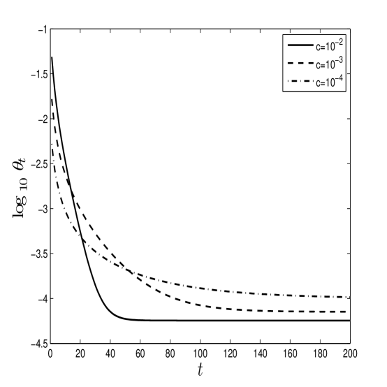
Figure 1: Plot of time varying parameter $\theta_{t}=\lambda_{t}^{-1}$ (logarithmic scale) for $c=10^{-2}$, $10^{-3}$ and $10^{-4}$.

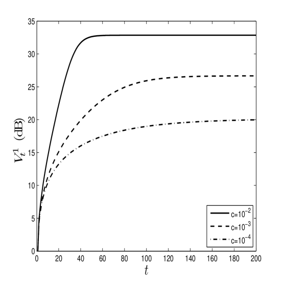
Figure 2: Error variance of $x_{1t}$ (dB scale) for $c=10^{-2}$, $10^{-3}$, and $10^{-4}$.

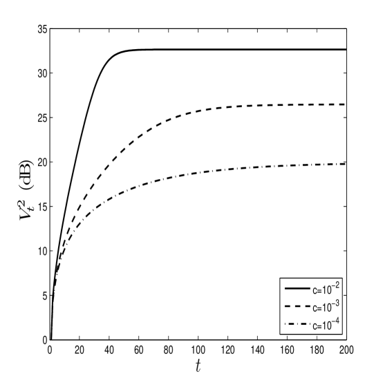
Figure 3: Error variance of $x_{2t}$ (dB scale) for $c=10^{-2}$, $10^{-3}$, and $10^{-4}$.

Next, for a tolerance $c=10^{-4}$, we compare the performance of the risk-sensitive and Kalman filters for the nominal model, and for the least-favorable model constructed as indicated in Section V. The variances of the two-states for the nominal model are shown in Fig. 4 and Fig. 5, respectively. Clearly, the loss of performance of the risk-sensitive filter compared to the Kalman filter is less than 1dB.

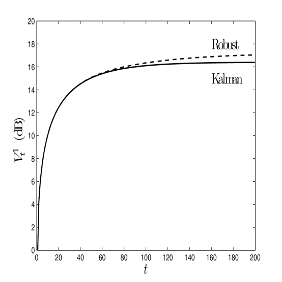
Figure 4: Error variance of $x_{1t}$ (dB scale) when the risk-sensitive filter with $c=10^{-4}$ and the Kalman filter are applied to the nominal model.

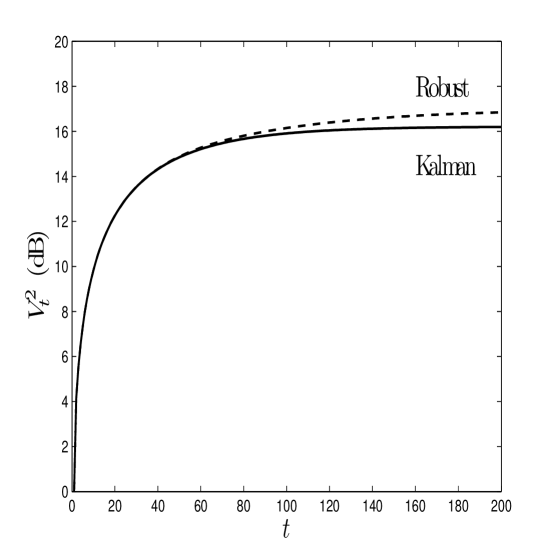
Figure 5: Error variance of $x_{2t}$ (dB scale) when the risk-sensitive filter with $c=10^{-4}$ and the Kalman filter are applied to the nominal model.

On the other hand, as indicated in Fig. 6 and Fig. 7, when the risk-sensitive and Kalman filters are applied to the least-favorable model, the Kalman filter performance is about 8dB worse than the robust filter. Note that to allow the backward recursion (5.13), (5.7) to reach steady state, the backward model is computed for a larger interval, and only the first 200 samples of the simulation interval are retained, since later samples are affected by transients of the least-favorable model.

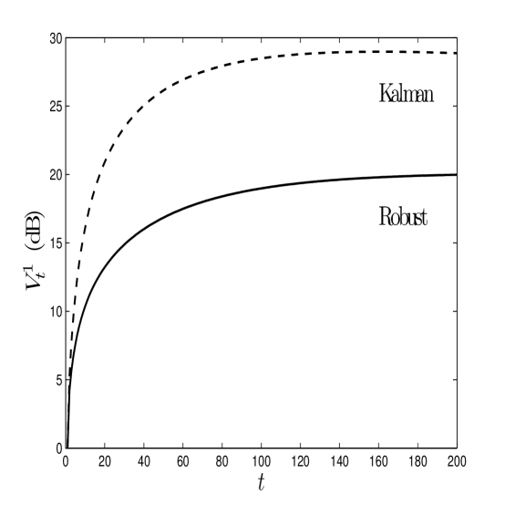
Figure 6: Error variance of $x_{1t}$ (dB scale) when the risk-sensitive filter with $c=10^{-4}$ and the Kalman filter are applied to the least-favorable model.

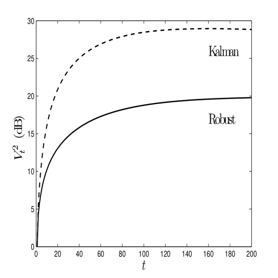
Figure 7: Error variance of $x_{2t}$ (dB scale) when the risk-sensitive filter with $c=10^{-4}$ and the Kalman filter are applied to the least-favorable model.

VII Conclusion

In this paper, we have considered a robust state-space filtering problem with an incremental relative entropy constraint. The problem was formulated as a dynamic minimax game, and by extending results presented in [1], it was shown that the minimax filter is a risk-sensitive filter with a time varying risk-sensitive parameter. The associated least-favorable model was constructed by performing a backward recursion which keeps track of retroactive probability changes made by the maximizing player. The results obtained are similar in nature to those derived by Hansen and Sargent [14, 15] for the minimax problem (3.25) when a single relative entropy constraint is applied to the overall state-space model and the maximizing agent is required to operate under commitment..

A number of issues remain to be resolved. For the case of a constant state-space model, it would be of interest to establish the convergence under appropriate conditions of the robust filtering recursions and of the backwards least-favorable model recursions. One also has to wonder if the results derived here for Gauss-Markov models could be extended to classes of systems, such as partially observed Markov chains, for which robust filtering with an overall relative entropy constraint was considered previously in [34].

References

• [1] B. C. Levy and R. Nikoukhah, “Robust least-squares estimation with a relative entropy constraint,” IEEE Trans. Informat. Theory, vol. 50, pp. 89–104, Jan. 2004.
• [2] P. J. Huber, Robust Statistics. New York: J. Wiley & Sons, 1981.
• [3] S. A. Kassam and T. L. Lim, “Robust Wiener filters,” J. Franklin Institute, vol. 304, pp. 171–185, 1977.
• [4] H. V. Poor, “On robust Wiener filtering,” IEEE Trans. Automat. Control, pp. 531–536, June 1980.
• [5] S. A. Kassam and H. V. Poor, “Robust techniques for signal processing: a survey,” Proc. IEEE, vol. 73, pp. 433–481, Mar. 1985.
• [6] J. L. Speyer, J. Deyst, and D. H. Jacobson, “Optimization of stochastic linear systems with additive measurement and process noise using exponential performance criteria,” IEEE Trans. Automat. Control, vol. 19, pp. 358–366, 1974.
• [7] P. Whittle, Risk-sensitive Optimal Control. Chichester, England: J. Wiley, 1980.
• [8] K. N. Nagpal and P. P. Khargonekar, “Filtering and smoothing in an $h^{\infty}$ setting,” IEEE Trans. Automat. Control, vol. 36, pp. 152–166, Feb. 1991.
• [9] D. Mustafa and K. Glover, Minimum Entropy $H^{\infty}$ Control. No. 146 in Lecture Notes in Control and Information Sciences, Berlin: Springer Verlag, 1990.
• [10] B. Hassibi, A. H. Sayed, and T. Kailath, Indefinite-Quadratic Estimation and Control– A Unified Approach to $H^{2}$ and $H^{\infty}$ Theories. Philadelphia: Soc. Indust. Appl. Math., 1999.
• [11] I. R. Petersen and A. V. Savkin, Robust Kalman Filtering for Signals and Systems with Large Uncertainties. Boston, MA: Birkhäuser, 1999.
• [12] A. H. Sayed, “A framework for state-space estimation with uncertain models,” IEEE Trans. Automat. Control, vol. 46, pp. 998–1013, July 2001.
• [13] L. El Ghaoui and G. Calafiore, “Robust filtering for discrete-time systems with bounded noise and parametric uncertainty,” IEEE Trans. Automat. Control, vol. 46, pp. 1084–1089, July 2001.
• [14] L. P. Hansen and T. J. Sargent, Robustness. Princeton, NJ: Princeton University Press, 2008.
• [15] L. P. Hansen and T. J. Sargent, “Robust estimation and control under commitment,” J. Economic Theory, vol. 124, pp. 258–301, 2005.
• [16] L. P. Hansen and T. J. Sargent, “Recursive robust estimation and control without commitment,” J. Economic Theory, vol. 136, pp. 1–27, 2007.
• [17] R. K. Boel, M. R. James, and I. R. Petersen, “Robustess and risk-sensitive filtering,” IEEE Trans. Automat. Control, vol. 47, pp. 451–461, Mar. 2002.
• [18] M.-G. Yoon, V. A. Ugrinovskii, and I. R. Petersen, “Robust finite horizon minimax filtering for discrete-time stochastic uncertain systems,” System & Control Let., vol. 52, pp. 99–112, 2004.
• [19] G. J. McLachlan and Krishnan, The EM Algorithm and Extensions. New York: Wiley, 1997.
• [20] N. N. Chentsov, Statistical Decision Rules and Optimal Inference, vol. 53 of Translations of Mathematical Monographs. Providence, RI: American Math. Society, 1980.
• [21] S.-I. Amari and H. Nagaoka, Methods of Information Geometry. Providence, RI: American Mathematical Society, 2000.
• [22] M. Basseville, “Information: Entropies, divergences et moyennes,” Tech. Rep. 1020, Institut de Recherche en Informatique et Systèmes Aléatoires, Rennes, France, May 1996.
• [23] J. R. Magnus and H. Neudecker, Matrix Differential Calculus with Applications in Statistics and Econometrics. Chichester, England: J. Wiley & Sons, 1988.
• [24] Y. Socratous, F. Rezaei, and C. D. Charalambous, “Nonlinear estimation for a class of systems,” IEEE Trans. Informat. Theory, vol. 55, pp. 1930–1938, Apr. 2009.
• [25] Y. Guo and B. C. Levy, “Robust MSE equalizer design for MIMO communication systems in the presence of model uncertainties,” IEEE Trans. Sig. Proc., vol. 54, pp. 1840–1852, May 2006.
• [26] B. C. Levy, A. Benveniste, and R. Nikoukhah, “High-level primitives for recursive maximum likelihood estimation,” IEEE Trans. Automat. Control, vol. 41, pp. 1125–1145, Aug. 1996.
• [27] R. A. Horn and C. R. Johnson, Matrix Analysis. New York: Cambridge University Press, 1985.
• [28] L. P. Hansen and T. J. Sargent, “Fragile beliefs and the price of uncertainty,” Quantitative economics, vol. 1, pp. 129–162, 2010.
• [29] J. P. Aubin and I. Ekland, Applied Nonlinear Analysis. New York: J. Wiley, 1984.
• [30] D. P. Bertsekas, A. Nedic, and A. E. Ozdaglar, Convex Analysis and Optimization. Belmont, Mass: Athena Scientific, 2003.
• [31] S. Kullback, Information Theory and Statistics. New York: J. Wiley & Sons, 1959. Reprinted by Dover Publ., Mineola, NY, 1968.
• [32] J. L. Speyer and W. H. Chung, Stochastic Processes, Estimation, and Control. Philadelphia, PA: Soc. Indust. Applied Math., 2008.
• [33] A. J. Laub, Matrix Anaysis for Scientists and Engineers. Philadelphia, PA: Soc. Indust. Applied Math., 2005.
• [34] L. Xie, V. A. Ugrinovskii, and I. R. Petersen, “Finite horizon robust state estimation for uncertain finite-alphabet hidden Markov models with conditional relative entropy constraints,” SIAM J. Control Optim., vol. 47, no. 1, pp. 476–508, 2008.